Pushing the limit of molecular dynamics with ab initio accuracy to 100 million atoms with machine learning

Abstract

For 35 years, ab initio molecular dynamics (AIMD) has been the method of choice for modeling complex atomistic phenomena from first principles. However, most AIMD applications are limited by computational cost to systems with thousands of atoms at most. We report that a machine learning-based simulation protocol (Deep Potential Molecular Dynamics), while retaining ab initio accuracy, can simulate more than 1 nanosecond-long trajectory of over 100 million atoms per day, using a highly optimized code (GPU DeePMD-kit) on the Summit supercomputer. Our code can efficiently scale up to the entire Summit supercomputer, attaining 91 PFLOPS in double precision (45.5% of the peak) and 162/275 PFLOPS in mixed-single/half precision. The great accomplishment of this work is that it opens the door to simulating unprecedented size and time scales with ab initio accuracy. It also poses new challenges to the next-generation supercomputer for a better integration of machine learning and physical modeling.

I Justification for Prize

Record molecular dynamics simulation of $>$100 million atoms with ab initio accuracy. Double/mixed-single/mixed-half precision performance of 91/162/275 PFLOPS on 4,560 nodes of Summit (27,360 GPUs). For a 127-million-atom copper system, time-to-solution of 8.1/4.6/2.7$\times 10^{-10}$ s/step/atom, or equivalently $0.8/1.5/2.5$ nanosecond/day, $>$1000$\times$ improvement w.r.t state-of-the-art.

II Performance Attributes

Performance attribute	Our submission
Category of achievement	Time-to-solution, scalability
Type of method used	Deep potential molecular dynamics
Results reported on basis of	Whole application including I/O
Precision reported	Double precision, mixed precision
System scale	Measured on full system
Measurements	Timers, FLOP count

III Overview of the Problem

III-A ab initio molecular dynamics

Molecular dynamics (MD) [1, 2] is an in silico simulation tool for describing atomic processes that occur in materials and molecules. The accuracy of MD lies in the description of atomic interactions, for which the ab initio molecular dynamics (AIMD) scheme [3, 4] stands out by evolving atomic systems with the interatomic forces generated on-the-fly using first-principles electronic structure methods such as the density functional theory (DFT) [5, 6]. AIMD permits chemical bond cleavage and formation events to occur and accounts for electronic polarization effects. Due to the faithful description of atomic interactions by DFT, AIMD has been the major avenue for the microscopic understanding of a broad spectrum of issues, such as drug discovery [7, 8], complex chemical processes [9, 10], nanotechnology [11], etc.

The computational cost of AIMD generally scales cubically with respect to the number of electronic degrees of freedom. On a desktop workstation, the typical spatial and temporal scales achievable by AIMD are $\sim$100 atoms and $\sim$10 picoseconds. From 2006 to 2019, the peak performance of the world’s fastest supercomputer has increased about 550-folds, (from 360 TFLOPS of BlueGene/L to 200 PFLOPS of Summit), but the accessible system size has only increased 8 times (from 1K Molybdenum atoms with 12K valence electrons  [12] to 11K Magnesium atoms with 105K valence electrons [13]), which obeys almost perfectly the cubic-scaling law. Linear-scaling DFT methods [14, 15, 16, 17] have been under active developments, yet the pre-factor in the complexity is still large, and the time scales attainable in MD simulations remain rather short.

For problems in complex chemical reactions [18, 19], electrochemical cells [20], nanocrystalline materials [21, 22], radiation damage [23], dynamic fracture, and crack propagation [24, 25], etc., the required system size typically ranges from thousands to hundreds of millions of atoms. Some of these problems demand time scales extending up to the microsecond and beyond, which is far out of the scope of AIMD. Although special simulation techniques that introduce a bias to enhance the sampling of the slow processes have been devised to deal with such situations [26, 27], they still require MD simulations of relatively long time scales on the order of tens or hundreds of nanoseconds. Some problems demand an even higher accuracy, e.g., the so-called chemical accuracy ($\sim$1 kcal/mol), than DFT could provide, requiring more expensive methods like CCSD(T) [28], whose computational complexity scales with the seventh power of the system size. Although there have been a host of empirical force fields (EFF)-based MD schemes (see, e.g., Refs. [29, 30, 31, 32, 33]), which can easily scale up to millions, or even trillions, of atoms, their accuracy is often in question. In particular, it has been challenging to develop EFFs for cases involving multiple elements or bond formation and cleavage, and for many practical problems there are no suitable EFFs available. Recently, reactive force fields capable of modeling chemical reactions, such as the REAXFF method introduced by Goddard and collaborators  [29, 33], have attracted considerable attention. These methods, however, lack the generality and predictive power of DFT. Above all, there is an urgent demand in the MD community for fundamentally boosting the efficiency of AIMD while keeping its accuracy.

III-B Deep Potential Molecular Dynamics

Recently, machine learning based MD (MLMD) schemes [34, 35, 36, 37, 38, 39, 40, 41] offer a new paradigm for boosting AIMD by means of ML-based models trained with ab initio data. One such model, Deep Potential (DP), has demonstrated the ability to achieve an accuracy comparable to AIMD, and an efficiency close to EFF-based MD [40, 41]. The accuracy of the DP model stems from the distinctive ability of deep neural networks (DNN) to approximate high-dimensional functions [42, 43], the proper treatment of physical requirements like symmetry constraints, and the concurrent learning scheme that generates a compact training dataset with a guarantee of uniform accuracy within the relevant configuration space [44].

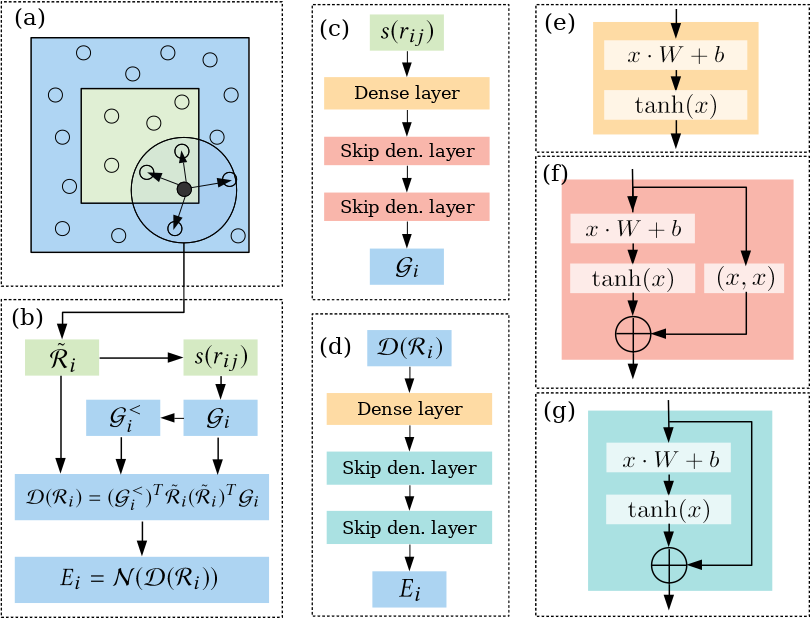
Figure 1: Schematic plot of the DP method. (a) A sub-region, including the local sub-region (green) and the ghost region (blue), handled by an MPI task. (b) Mapping of the local environment of a single atom onto atomic energy contribution. (c) Structure of the embedding net. (d) Structure of the fitting net. (e) Dense layer used in the embedding net. (f) Skip connected dense layer used in the embedding net. (g) Skip connected dense layer used in the fitting net.

As shown in Fig. 1, to construct a DP model, first, the coordinates of atom $i$ and of its neighboring atoms are converted to the descriptors $\mathcal{D}$, which encode the local atomic environment through a set of symmetry preserving features and trainable parameters. Next, the descriptors are passed to the fitting net, a fully connected DNN denoted by $\mathcal{N}$, which outputs the atomic energy contribution $E_{i}$. Finally, the potential energy is constructed as the summation of $E_{i}$. In detail, the descriptor $\mathcal{D}$ is the product of terms involving the environment matrix $\tilde{\mathcal{R}}$, which faithfully records the relative positions of the neighbors, and the embedding matrix ${\mathcal{G}}$, which encodes the information of the distances between atoms by a DNN named embedding net. The dependence of DP on the atomic coordinates is continuous to at least the 2nd order in the atomic displacements. The training of the DP model has been implemented in the DeePMD-kit package [45]. The typical training time spans from several hours to one week on a single GPU card, depending on the complexity of the data.

TABLE I: Performance of molecular dynamics simulators with ab initio accuracy. The abbreviations Pot., TtS, LS, BP, and DP stand for potential, time-to-solution, linear scaling, Behler-Parrinello scheme, and Deep Potential, respectively. In AIMD, we assume 5 electronic steps for each MD (ionic) step. The time-step of water system is 0.5 fs, and that of other systems is 1 fs. *The parallel efficiency does not significantly decay at the largest machine scale tested in the work, so it is highly likely that they can scale to larger machines. $\dagger$Vienna Scientific Cluster (VSC), an HPC system with Intel Xeon Gold 6138 CPUs. $\ddagger$An unknown cluster with Intel Xeon E5-2650v2 CPUs at the KISTI supercomputing center. **The baseline DeePMD-kit implementation.

Work	Year	Pot.	System	#atoms	#CPU cores	#GPUs	Machine	Peak[FLOPS]	TtS [s/step/atom]
Qbox [12]	2006	DFT	Mo	1K	262K	–	BlueGene/L	207T	$2.8$ $\times$	$10^{-1}$
LS3DF [14]	2008	LS-DFT	ZnTeO	16K	131K	–	BlueGene/P	108T	$1.8$ $\times$	$10^{-2}$
RSDFT [46]	2011	DFT	Si	107K	442K	–	K-computer	3.1P	$2.6$ $\times$	$10^{0}$
DFT-FE [13]	2019	DFT	Mg	11K	159K	22.8K	Summit	46P	$6.5$ $\times$	$10^{-2}$
CONQUEST [17]	2020	LS-DFT	Si	1M	200K	–	K-computer	?	4.0 $\times$	$10^{-3}$
Simple-NN [47]*	2019	BP	SiO2	14K	80	–	Unknown$\ddagger$	?	$3.6$ $\times$	$10^{-5}$
Singraber el.al. [48]*	2019	BP	H2O	9K	512	–	VSC$\dagger$	?	$1.3$ $\times$	$10^{-6}$
Baseline [45]**	2018	DP	H2O	25K	1	1	Summit	–	$5.6$ $\times$	$10^{-5}$
This work (double)	2020	DP	H2O	679M	27.3K	27.3K	Summit	80P	$3.0$ $\times$	$10^{-10}$
This work (mixed-half)	2020	DP	H2O	679M	27.3K	27.3K	Summit	212P	$1.1$ $\times$	$10^{-10}$
This work (double)	2020	DP	Cu	127M	27.3K	27.3K	Summit	91P	$8.1$ $\times$	$10^{-10}$
This work (mixed-half)	2020	DP	Cu	127M	27.3K	27.3K	Summit	275P	$2.7$ $\times$	$10^{-10}$

Deep Potential Molecular Dynamics (DeePMD) has greatly boosted the time and size scales accessible by AIMD without loss of ab initio accuracy. To date, DeePMD has been used to model various phenomena in physical chemistry [49, 50, 51, 52, 53] and materials sciences [54, 55, 56, 57, 58, 59]. For example, in a recent work [49], DeePMD was used to simulate the TiO₂-water interface, providing a microscopic answer to an unsolved question in surface chemistry: do water molecules dissociate or remain intact at the interface between the liquid and TiO₂? In another recent work [58], DeePMD was used in combination with experiments to show the mechanism behind the nucleation of strengthening precipitates in high-strength lightweight aluminium alloys. These examples are challenging for AIMD due to the spatial and temporal limits of this approach. They are also difficult, if not impossible, for EFF-based MD schemes, due to the limited capability of the relatively simple form of the potential energy function they adopt.

IV Current state of the art

An important goal of molecular simulation is to model with ab initio accuracy realistic processes that involve hundreds of millions of atoms. To achieve this goal, major efforts have been made to boost AIMD without loss of accuracy. Some examples are QBox [12], LD3DF [14], RSDFT [46], DFT-FE [13], and CONQUEST [17]. Their performances are summarized in Table I, where the system size, the peak performance, the time-to-solution, etc., are provided. We observe that it is challenging for conventional DFT-based AIMD schemes to overcome the cost limits even with the fastest available HPCs. As a rough estimate, assuming that future HPC performance will continue to improve at the same pace as in the past fourteen years, it would take several decades to be able to model the target size and time scales of interest with conventional AIMD techniques.

The MLMD schemes mentioned in the last section offer a chance to bypass the conventional AIMD methods without losing their accuracy. Representative examples are the Behler-Parrinello scheme [34], the Gaussian approximation potential [35, 60], SchNet [37], and the Deep Potential method [39, 40]. Up to now, most attentions of the community have been devoted to improving the representability and transferability of the machine learning schemes, and to solving scientific problems that do not really require very large-scale MD simulations. Efforts on implementation and optimization with an HPC perspective have remained at an early stage. Some open-source packages for the MLMD schemes have been released: the QUantum mechanics and Interatomic Potentials (QUIP) [61], Amp [62], DeePMD-kit [45], TensorMol [63], SIMPLE-NN [47], PES-Learn [64], and a library-based LAMMPS implementation of neural network potential [48]. The performance reported in these works, if any, is summarized in Table  I. It is observed that existing implementations of MLMD are basically for desktop GPU workstations or CPU-only clusters. None of them can fully utilize the computational power offered by the accelerators on modern heterogeneous supercomputers.

Of particular relevance to our work is the DeePMD scheme, which has been implemented in an open-source package called DeePMD-kit [45]. DeePMD-kit is built on the MD platform LAMMPS [65] and the deep learning platform TensorFlow [66]. By interfacing the DP model with LAMMPS, which maintains the atomic information and integrates the equations of motion, the key function of DeePMD-kit is to implement the calculation of atomic energies and forces predicted by the DP model. With TensorFlow, a versatile tool box for deep learning, the embedding matrix, the descriptors, and the atomic energy are implemented by standard operators built in TensorFlow. Moreover, TensorFlow provides GPU support for its standard operators, thus the corresponding calculations in DeePMD-kit are easily accelerated with GPU by linking to the GPU TensorFlow library. Unfortunately, the implementation of DeePMD-kit cannot fully utilize the computational power of modern heterogeneous supercomputers like Summit, due to the following restrictions: (1) The code is designed on single node with only single GPU serial or multi-CPU OpenMP parallelism [45]. (2) The customized TensorFlow operators introduced for the environment matrix, force, and virial are implemented only on CPUs. (3) The size of the DNN used by DP models is typically smaller than the sizes adopted in normal deep learning applications like pattern detection and language processing, which implies that each individual step of a computationally intensive operation is also smaller in DP applications. In this context, the memory bandwidth and latency become obstacles to improving the computational efficiency of the DeePMD-kit package. To summarize, large-scale DeePMD simulations with ab initio accuracy have been only conceptually proved to be possible, but have never been made practically accessible by a code optimized for modern heterogeneous HPCs, from both algorithmic and implementation perspectives.

Above all, to the best knowledge of the authors, efficient MD simulation of 100 million atoms with ab initio accuracy has never been demonstrated with AIMD or MLMD schemes. We believe that to make this goal a routine procedure, we need to pursue integration of physics-based modeling, machine learning, and efficient implementation on the next-generation computational platforms. In the following sections, we shall adopt the serial DeePMD-kit [45] as the baseline DeePMD implementation and demonstrate how its performance can be greatly boosted on Summit.

V Innovations

V-A Summary of contributions

Our major contribution is a highly efficient and highly scalable method for performing MD simulation with ab initio accuracy. This is achieved by combining the unprecedented representation capability of the DP model (Figs. 2 (a)-(b)), and a highly scalable and fine-tuned implementation on heterogeneous GPU architectures (Figs. 2 (c)-(g)). The resulting optimized DeePMD-kit scales almost perfectly up to 4,560 computing nodes on Summit for a copper system of 127,401,984 atoms, reaching $91$ PFLOPS in double precision, and $162$ and 275 PFLOPS in mixed single and mixed half precision, respectively. The corresponding time-to-solution is $34$ milliseconds per MD step with mixed half precision, outperforming existing work by more than three orders of magnitude and enabling nanosecond simulation within $10$ hours.

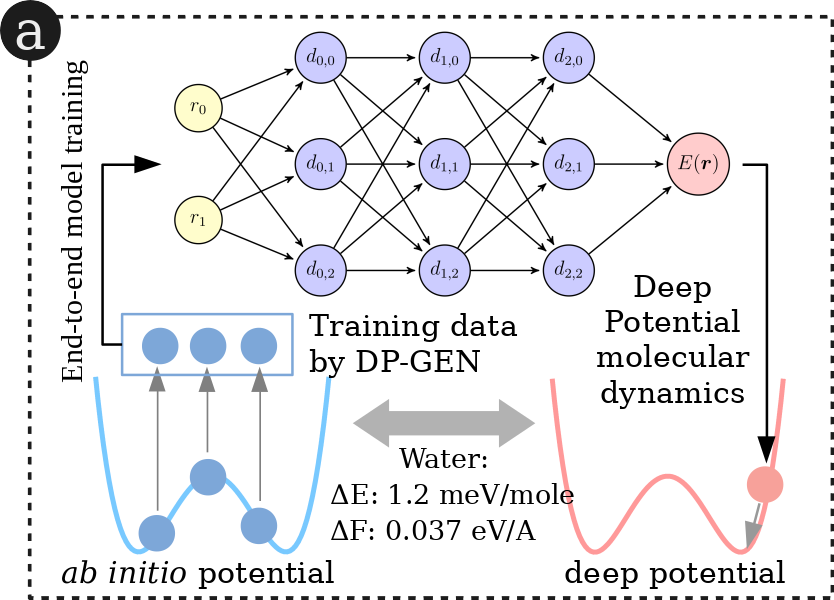
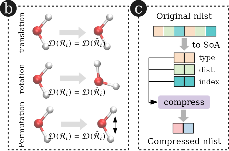
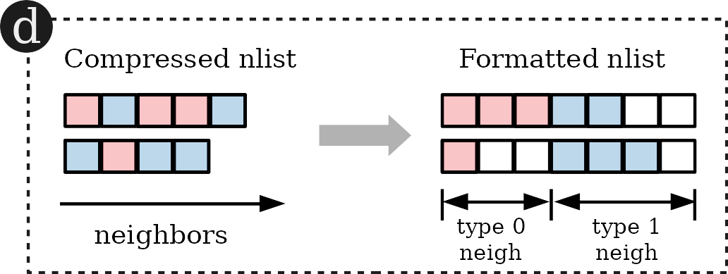
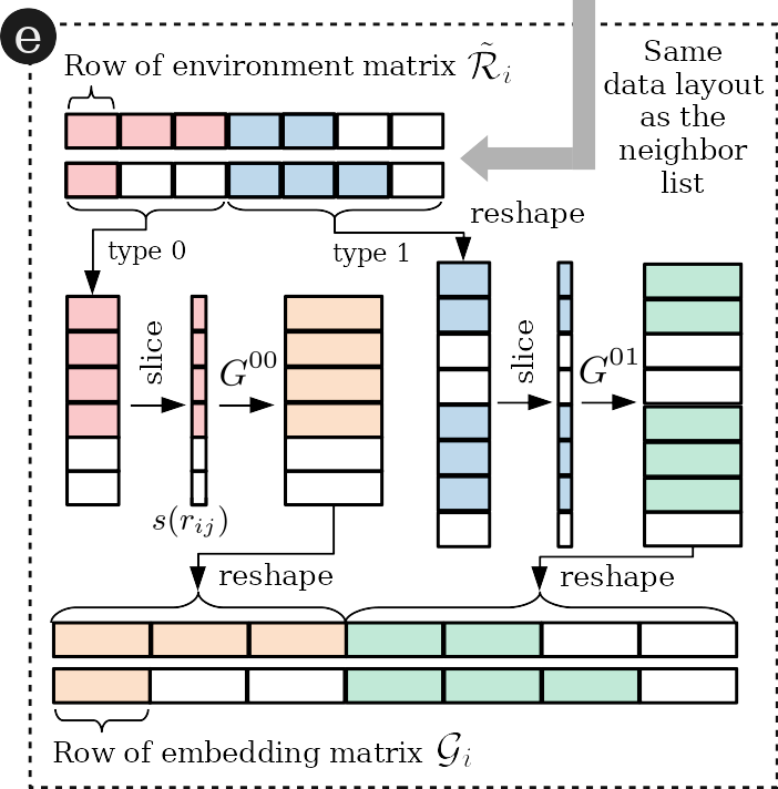
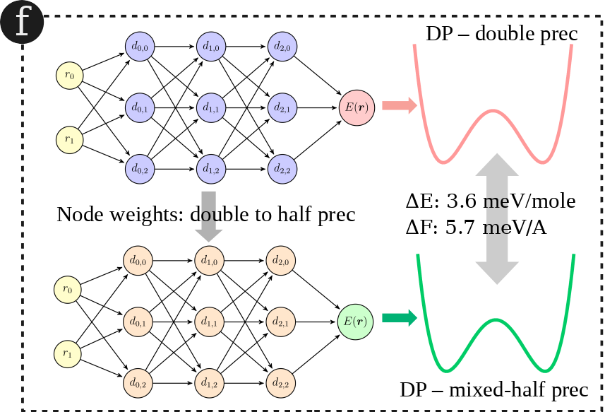
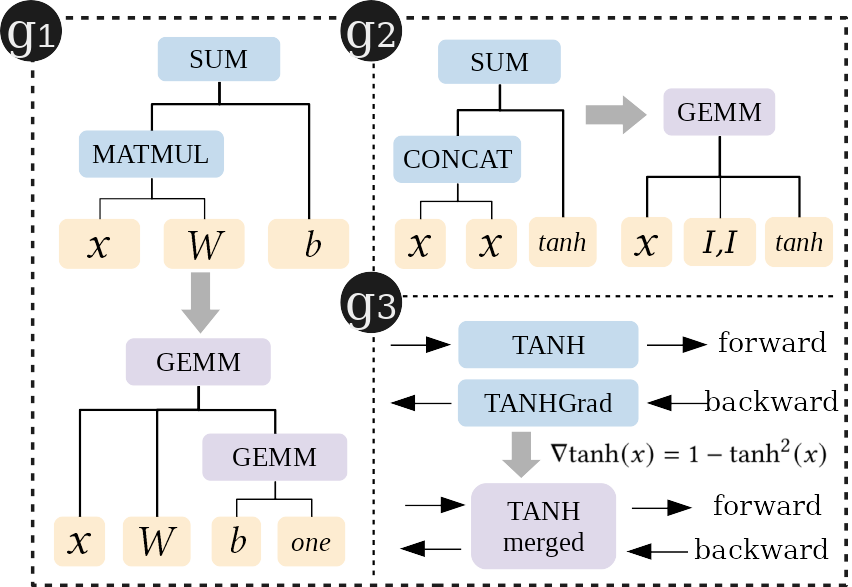
Figure 2: Key steps in the optimized DeePMD-kit, taking water as an example.

V-B Algorithmic innovation

To effectively harness the computing power offered by the heterogeneous system architecture of Summit, our goal is to migrate to GPUs almost all computational tasks and a significant amount of communication tasks. Due to the relatively limited size of the computational granularity in the DP model, a straightforward GPU implementation encounters many bottlenecks and is thus not efficient. As such, our main algorithmic innovations are the following:

• We increase the computational granularity of DeePMD by introducing a new data layout for the neighbor list that avoids branching in the computation of the embedding matrix.

• The elements in the new data structure of the neighbor list are compressed into 64-bit integers for more efficient GPU optimization of the customized TensorFlow operators.

• We develop mixed-precision computation for the DP model. Computationally intensive tasks are performed with single or half precision without reducing the accuracy of the physical observables.

V-B1 Increasing computational granularity

The novelty of the DP model lies in its ability to automatically generate a set of symmetry-preserving descriptors $\mathcal{D}$ through the embedding net (Figs. 1 (b) and (c)) from the local environment of each atom described by the environment matrix $\mathcal{R}_{i}$. By using roughly the same set of hyper-parameters, DP can fit the data for almost all tested systems. Compared to other methods with fixed feature sets, DP is more versatile when facing complex data, e.g., multi-component systems, chemical reactions, etc. Since important symmetries are strictly preserved in $\mathcal{D}$ (see Fig. 2 (b)), a fitting network of three layers (see Fig. 1 (d)) is enough to produce results with high fidelity.

The most computationally intensive part of the DP model is the embedding matrix. The pattern of the computation is defined by the order of neighbors recorded in the neighbor list. We notice that since the descriptors are permutationally invariant (Fig. 2 (b)), neighbor lists with different orders are equivalent in terms of accuracy. By taking advantage of this observation, we redesign the data layout of the neighbor list by sorting the neighbors according to their type, and, within each type, we sort the neighbors by their relative distance. The neighbors of the same type are padded to the cut-off number of neighbors corresponding to that type (Fig. 2 (d)). The first sorting (according to neighbor types) and the padding align the neighbors with the same type, so the conditional branching according to the type of the neighbors in the embedding matrix computation is avoided (see Fig. 2 (e)). This greatly increases the computational granularity, a critical component for taking advantage of the computational power offered by GPUs. The second sorting always selects the neighbors in the list according to their distance from the central atom. In this way, if the number of neighbors occasionally fluctuates beyond $N_{max}$, the cut-off number of neighbors defined in the padding step, only information on the nearest neighbors up to $N_{max}$ is retained, avoiding the unphysical phenomena that would occur if close neighbors were neglected.

V-B2 Optimization of Customized TensorFlow Operators

In this part, we present the optimization of the customized TensorFlow operators, which take more than $84\%$ of the total computational cost in the baseline DeePMD-kit. We start from formatting the neighbor list, whose data layout is crucial and discussed in Sec. V-B1. Each element of the neighbor list is a structure with 3 data items: the atomic type $\alpha(j)$, the atomic distance $|r_{ij}|$, and the atomic index $j$ (Fig. 2 (c)). In the formatting process, the neighbor list is sorted first based on the atomic type, then based on the atomic distance $|r_{ij}|$.

The AoS (Array of structures) data layout of the neighbor list makes it impossible for efficient memory access on GPU because of memory coalescing problems. One common practice in GPU optimization is to switch from AoS to SoA (Structure of arrays). However, in DeePMD-kit, we propose an even more efficient way of storing the neighbor list by compressing each element of the neighbor list into a 64-bit unsigned integer (Fig. 2 (c)) with the following equation: $\alpha(j)\times 10^{16}+\lfloor|r_{ij}|\times 10^{8}\rfloor\times 10^{6}+j$. The 20 decimal digits of the 64-bit unsigned integer are divided into 3 parts to store the one element of neighbor list: 4 digits for the atomic type, 10 digits for the atomic distance, and 6 digits for the atomic index. The range of all the three parts are carefully chosen and are rarely exceeded in typical DeePMD simulations. Both the compression before sorting and the decompression after sorting are accelerated via CUDA customized kernels, so that the corresponding computational time is negligible. Sorting the compressed neighbor list reduces the number of comparisons by half with no impact on the accuracy of the algorithm, and is carried out by calling the NVIDIA CUB library, which provides the state-of-the-art and reusable software components for each layer of the CUDA programming model, including block-wide sorting.

According to Amdahl’s law, an ideal overall speedup can only be achieved by accelerating all calculations. In our implementation, all customized TensorFlow operators, Environment, ProdForce, and ProdViral, which compute the environment matrix, force, and the virial, respectively, are migrated and optimized on the GPU. In particular, a fine-grained parallelism is utilized to exploit the computing power of the GPU.

Now that all computationally intensive tasks are carried out by the GPU, we further reduce the time for GPU memory allocation by allocating a trunk of GPU memory at the initialization stage, and re-using the GPU memory throughout the MD simulation. The CPU-GPU memory copy operations are also optimized to eliminate non-essential data transfer processes.

V-B3 Mixed-precision computation

The approximation property of the DNN-based DP model provides us with an opportunity for mixed-precision calculations. In the optimized code, different levels of mixed precision are tested, and we find that two prescriptions of mixed precision are of satisfactory stability and accuracy. Both of them use double precision for atomic positions and the environment matrix construction. In the MIX-32 scheme, all parameters of the embedding net and fitting net are stored in single precision (32-bit). The environment matrix is converted from double precision to single precision, then all the arithmetic operations of the embedding net and the fitting net are performed in single precision. In the MIX-16 scheme, the parameters of the embedding net and the first two fitting net layers are stored in half precision (16-bit). The environment matrix is cast to half precision and then fed to the embedding net. In each embedding net layer and the first two fitting net layers, the GEMM operations are performed using Tensor Cores on V100 GPU with accumulations in single precision, except for those in the first embedding net layer that do not meet the size requirements for using Tensor Cores. All other floating point operations, such as TANH and TANHGrad, are conducted in single precision due to accuracy considerations. The data are cast to half precision before writing the global memory. Note that in the last layer of the fitting net, both data storage and arithmetic operations are kept in single precision, which is critical to the accuracy of the MIX-16 scheme. Finally, the outputs of the fitting net of MIX-32 and MIX-16 are converted back to double precision, and the total energy of the system is reduced from the atomic contributions. The model parameters $W$ and $b$ are trained in double precision, and cast to single and half precision in the MIX-32 and MIX-16 schemes, respectively.

We compare the mixed-precision schemes with the double precision by using a typical configuration of a water system composed of 512 molecules. With MIX-32 we observe a deviation of $5.2\times 10^{-6}$ eV (normalized by the number of molecules) in the energy prediction and a root mean square deviation of $2.5\times 10^{-6}$ eV/Å in the force prediction, which indicates an excellent agreement with the double precision scheme. With MIX-16 we observe a deviation of $3.6\times 10^{-3}$ eV (normalized by number of molecules) in the energy prediction and a root mean square deviation of $5.7\times 10^{-3}$ eV/Å in the force prediction. The deviation in the force prediction is significantly smaller than the training error ($\sim$4$\times$$10^{-2}$ eV/Å). The deviation in energy prediction is comparable to the training error, but is already much smaller than the chemical accuracy ($\sim$4$\times 10^{-2}$ eV/molecule). The accuracy of the mixed-precision schemes in predicting physical observables is further validated in Sec. VII-A3.

V-C Neural Network Innovation

After optimizing customized TensorFlow operators (Sec. V-B2), the remaining computational cost is dominated by standard TensorFlow operators. The floating point operations are dominated by operators like MATMUL (matrix-matrix multiplication) and TANH (activation function). Other operators such as CONCAT (matrices concatenation) and SUM (matrix addition) are bandwidth intensive and cost few floating point operations. We find that many operations in DeePMD-kit involve matrix-matrix multiplication of tall and skinny matrices. This leads to particularly large overheads in the operations like SUM, so standard TensorFlow operators are not optimized to treat such matrices efficiently. Through detailed performance profiling, we redesign several operations in the execution graph of TensorFlow. Although these are tailored operations designed to improve the efficiency of DeePMD-kit, similar strategies should be useful in other machine learning applications, particularly those integrated with physical modeling.

V-C1 Replace MATMUL and SUM Operators with GEMM

In the standard TensorFlow execution graph, the operation $x\cdot W+b$ (see Fig. 1 (e-g)) is implemented with two separate operators: MATMUL and SUM. For example, for the oxygen-hydrogen pairs in a water system with 4,096 molecules, MATMUL in the last layer of the embedding net multiplies $x$ of size 786,432 $\times$ 64 with $W$ of size ${64}\times{128}$. Then the SUM operator adds the bias $b$ to each row of $x\cdot W$. In many data-driven applications the sizes of matrices $x$ and $W$ are large enough so that the overhead of the SUM is negligible compared to that of the MATMUL operator. However, in the case of DeePMD, the second dimension of $x$ and the size of $W$ are relatively small, so the cost of SUM becomes important. In the optimized computational graph, we replace the MATMUL and SUM operators with a single CUBLAS GEMM call. Note that the vector $b$ is converted to a matrix before SUM by right multiplying with the transpose of vector one (Fig. 2 (g1)).

V-C2 Replace CONCAT and SUM Operators with GEMM

In the standard TensorFlow computational graph, the operation $(x,x)+...$ (see Fig. 1 (f)) is implemented by a CONCAT operator that concatenates two $x$s to form $(x,x)$ and a SUM operator that adds $(x,x)$ to the output of the TANH operator. We optimize this operation by replacing CONCAT with a matrix-matrix multiplication $(x,x)\rightarrow x\times(I,I)$, and merging this multiplication with SUM to form a CUBLAS GEMM call (Fig. 2 (g2)). We observe that the multiplication is only marginally faster than CONCAT, and the benefit comes from the merging of the SUM.

V-C3 CUDA kernel fusion for the TANH and TANHGrad

TANH is the activation function (see Fig. 1 (e-g)), while TANHGrad (not explicitly shown in Fig. 1) is the derivative of the output of TANH w.r.t the input for backward propagation. We need both TANH and TANHGrad in each MD step to evaluate the forces. We observe that the derivative of $\tanh(x)$ is also a function of $\tanh(x)$, i.e. $\nabla{\tanh(x)}=1-{\tanh^{2}(x)}$. Thus, in the optimized DeePMD-kit, both TANH and TANHGrad operators are implemented in one CUDA customized kernel to save computational time (Fig. 2 (g3)). Since the GPU memory of the TANHGrad is allocated in the forward propagation, this optimization is essentially trading space for time.

V-D Reducing MPI communication bottlenecks

Despite the multi-body nature of DP, due to its force decomposition scheme, we can adopt for DP the same parallelization scheme of the EFFs implemented in LAMMPS (Fig. 1 (a)). The computation of EFFs in LAMMPS is replaced by the computation of DP, and LAMMPS is also used to maintain the spacial partitioning of the system and all the communications between sub-regions.

There are mainly two types of MPI communications in each DeePMD step: the communication of the ghost region between adjacent MPI tasks and the global reduction for the physical properties. In our implementation, we optimize the communication of the ghost region using the CUDA-aware IBM Spectrum MPI, since it resides on the GPU in the calculation. When the output information is required, MPI_Allreduce operations across all MPI tasks are performed to collect physical properties, such as total energy, pressure, etc.. Although each of these physical properties is only one double precision number and the corresponding MPI_Allreduce operation is latency dominated, the scaling of the optimized DeePMD-kit is hindered by the implicit MPI_Barrier in extremely large-scale calculations. To alleviate this problem, we reduce the output frequency to every 20 steps, a common practice in the MD community. In addition, we replace the MPI_Allreduce with MPI_Iallreduce to further avoid the implicit MPI_Barrier.

VI Performance measurement

VI-A Physical Systems

Among various complex physical systems that have been described by DP, we choose two typical and well-benchmarked systems, one insulating (water) and one metallic (copper), to measure the performance of the optimized DeePMD-kit. Water is a notoriously difficult system even for AIMD, due to the delicate balance between weak non-covalent intermolecular interactions,thermal (entropic) effects, as well as nuclear quantum effects [67, 68, 53]. We have shown in Refs. [40, 53] that DeePMD can accurately capture such effects in water. In combination with extensions of the DP formulation to vectors and tensors, the infra-red [52] and Raman [69] spectra of water have been properly described. Copper is a representative simple metal, yet a lot of its properties, such as the surface formation energy and stacking fault energies, can be hardly produced well by EFFs. In Ref. [70], using a concurrent learning scheme [44], we have generated an optimal set of ab initio training data and realized a DP model for copper with a uniform accuracy over a large thermodynamic region.

For water and copper, the cut-off radii are 6 Å and 8 Å and the cut-off numbers of neighbors are 144 and 512, respectively. The fitting nets of the models are of size ($240,240,240$), and the embedding nets are of size ($32,64,128$). To test the performance, the MD equations are numerically integrated by the velocity-Verlet scheme for 500 steps (the energy and forces are evaluated for 501 times) at time-steps of 0.5 fs (water) and 1.0 fs (copper). The velocities of the atoms are randomly initialized subjected to the Boltzmann distribution at 330 K. The neighbor list with a 2 Å buffer region is updated every 50 steps. The thermodynamic data, including kinetic energy, potential energy, temperature, pressure, are collected and recorded every 20 time-steps.

For the water system, the strong scaling tests are performed on a system with 4,259,840 molecules (12,779,520 atoms). The total number of floating point operations for 500 MD steps of this system is $151.1$ PFLOPs. Weak scaling tests ranging from 42,467,328 to 679,477,248 atoms are performed on up to 4,560 computing nodes on Summit. We notice that compared with the water system, the copper system, with the same number of atoms, has $3.5$ times more floating point operations. The strong scaling tests of the copper system are carried out with a system of 15,925,248 atoms. The total number of floating point operations for 500 MD steps of this system is $588.7$ PFLOPs. The weak scaling tests are performed on up to 4,560 computing nodes of Summit for systems ranging from 7,962,624 to 127,401,984 atoms.

Since the baseline DeePMD-kit is restricted by its sequential implementation and can run none of these systems, a fraction of the water system (12,288 atoms/4096 water molecules) is used for comparison with the optimized code on a single GPU in Sec. VII-A.

VI-B HPC Platforms and Software Environment

All the numerical tests are performed on the Summit supercomputer, which consists of 4,608 computing nodes and ranks No. $2$ on the TOP500 list for a peak performance of 200 PFLOPS [71]. Each computing node has two identical groups, each group has one POWER 9 CPU socket and 3 NVIDIA V100 GPUs and they are interconnected via NVLink. The total computing power for a single node is 43 TFLOPS in double precision (each V100 GPU $7$ TFLOPS and each POWER 9 socket $515$ GFLOPS, thus 7$\times$6$+$2$\times$0.5=43 TFLOPS in total), 86 TFLOPS in single precision, and 720 TFLOPS in half precision with Tensor Cores (120 TFLOPS per GPU). Each computing node has 512 GB host memory and $96$GB ($16$GB per GPU) GPU memory. The CPU bandwidth is 135 GB/s (per socket) and GPU bandwidth is 900 GB/s (per GPU). The two groups of hardware are connected via X-Bus with a 64 GB/s bandwidth. The computing nodes are interconnected with a non-blocking fat-tree using a dual-rail Mellanox EDR InfiniBand interconnect with a total bandwidth of 25 GB/s.

TABLE II: Software environment

Name	Module used
MPI	IBM Spectrum MPI 10.3.1.2-20200121
Host compiler	GCC 4.8.5
GPU compiler	CUDA 10.1.168
TensorFlow	IBM-WML-CE 1.6.2-2 (TensorFlow 1.15 included)

The software environment is listed in Table  II. In all tests, a single OpenMP thread is used. We use 6 MPI tasks per computing node (3 MPI tasks per socket to fully take advantage of both CPU-GPU affinity and network adapter), and each MPI task is bound to an individual GPU.

VI-C Measurements

The total number of floating point operations (FLOPs) of the systems is collected via the NVIDIA CUDA NVPROF tool. We remark that NVPROF only gathers the FLOPs on the GPU. However, in DeePMD-kit, all computationally intensive calculations are performed on the GPU, thus the total FLOPs is reasonable. Both double-precision and mixed-precision results are reported in Sec. VII. The following three criteria are used to measure the performance of the DeePMD-kit.

• Time-to-solution, defined as $\frac{\textsf{MD loop time}}{\textsf{number of MD steps}}$, the average wall clock time used for calculating a single MD step . The “MD loop time” includes all the time used in the MD loop (IO included). Setup time, such as the setup of the system and MPI initialization and finalization, is not included.

• Peak performance, defined as $\frac{\textsf{total FLOPs}}{\textsf{MD loop time}}$.

• Sustained performance, defined as $\frac{\textsf{total FLOPs}}{\textsf{total wall clock time}}$. The “total wall clock time” includes the whole application running time (including IO).

VII Performance Results

VII-A Single GPU

In the following, taking the double-precision implementation as an example, we discuss our optimizations on the customized and standard TensorFlow operators in Secs. VII-A1 and VII-A2, respectively. Then we discuss the implementation of mixed precision and the overall performance in Sec. VII-A3.

VII-A1 Customized TensorFlow operators

We optimize the customized TensorFlow operators with CUDA customized kernels according to Sec. V-B2. In the baseline implementation, the customized TensorFlow operators take about 85% of the total MD loop time for a water system of 12,288 atoms. The performance of the customized operators of the baseline and optimized implementations are compared in Table  III. For all the customized TensorFlow operators, an overall speedup of $64.6$ times is achieved. Moreover, a total speedup factor of $6.2$ is reached for the “MD loop time”.

TABLE III: Performance of optimized customized TensorFlow operators. Baseline customized operators are implemented on CPU.

Operators	Baseline[ms]	Optimized[ms]	Speedup
Environment	$302.54$	$2.32$	$130$
ProdViral	$51.06$	$1.34$	$38$
ProdForce	$41.29$	$2.41$	$17$

VII-A2 Standard TensorFlow operators

Some of the standard TensorFlow operators are re-implemented and optimized according to Sec. V-C. For the water system of 12,288 atoms, MATMUL+SUM, CONCAT+SUM, and TANH+TANHGrad in the baseline implementation are accelerated by 1.3, 1.7, and 1.6 times with GEMM, GEMM, and merged TANH , respectively. The baseline implementation calls standard TensorFlow operators, which are already highly efficient on GPUs, yet an extra $1.21$ times of speedup is achieved for the “MD loop time” compared with Sec. VII-A1.

VII-A3 Mixed precision

TABLE IV: Test errors for the water system from models with different precision.

Precision	Error in energy [eV/molecule]	Error in force [eV/Å]
Double	$1.2\times 10^{-3}$	$3.7\times 10^{-2}$
MIX-32	$1.2\times 10^{-3}$	$3.7\times 10^{-2}$
MIX-16	$3.6\times 10^{-3}$	$3.8\times 10^{-2}$

The accuracy of the mixed precision models is investigated by comparing the energy and forces computed from DeePMD-kit with those from AIMD predictions. We take water as an example and the test data set is composed of 100 water configurations of 64 molecules. As shown in Table IV, the MIX-32 scheme is as accurate as the double precision. The accuracy of MIX-16 is slightly worse than that of the double precision model, but is usually enough for an accurate prediction of physical observables. To further check the accuracy, we calculate the radial distribution function (RDF), the normalized probability of finding a neighboring atom at the spherically averaged distance $r$. The oxygen-oxygen ($g_{OO}(r)$), oxygen-hydrogen ($g_{OH}(r)$), and hydrogen-hydrogen ($g_{HH}(r)$) RDFs are typically utilized to characterize the structures of water [40]. As shown in Fig. 3, the RDFs computed from the mixed-precision implementations (MIX-32 and MIX-16) agree perfectly with those from the double-precision implementation and those from the AIMD calculation. Therefore, we conclude that the mix-precision methods do not lead to loss of accuracy for predicting physical observables.

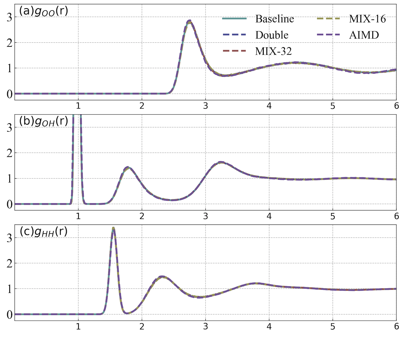
Figure 3: Radial distribution functions $g_{OO}(r)$, $g_{OH}(r)$, and $g_{HH}(r)$ of liquid water at ambient conditions, calculated by AIMD and four DeePMD-kit implementations: baseline, optimized double, MIX-32, and MIX-16.

For the water system, compared with the double-precision version, the MIX-32 code is about $1.7$ times faster and saves half of the GPU memory cost, and the MIX-16 code is $2.6$ times faster and saves  $75\%$ of the GPU memory cost. Together with the speedups from Secs. VII-A2 and  VII-A1, it is concluded that the optimized DeePMD-kit with double precision is around 7.5 times faster than the baseline code, and the speedup factor increases to 12.7 and $19.5$ when the MIX-32 and MIX-16 codes are used.

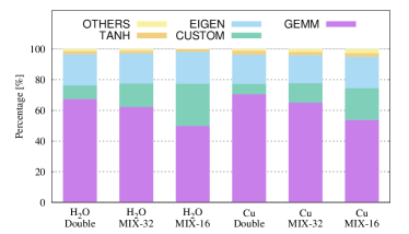
Figure 4: Percent stacked bar chart of different TensorFlow operators in terms of the GPU computational time for $24,576$ and $4,860$ atoms for water and copper, respectively.

Finally, Fig.  4 shows the percentage of time spent by different TensorFlow operators in the total GPU execution time. We notice that the contribution from the GEMM operator is more important in the copper system (double: $71\%$, MIX-32: $65\%$ MIX-16: $54\%$) than that in the water system (double: $67\%$, MIX-32: $62\%$, MIX-16: $50\%$). This is mainly attributed to the fact that the FLOPs of the copper system is $3.5$ times bigger than that of the water due to the larger number of neighbors per atom, as discussed in Sec. VI-A. We remark that the GEMM operator in DeePMD-kit is still memory-bound due to the the small network size (the dimensions of the three embedding network layers are 32, 64, and 128). Profiling on the water system shows that the average computational efficiency of the GEMM operations is $66.4\%$, $62.3$ and $19.3\%$ for double, MIX-32, and MIX-16 versions, respectively. The corresponding bandwidth utilization is $88.9\%$, $88\%$ and $87.6\%$ of the hardware limit, respectively. As the network size grows, the bandwidth limitation will be alleviated. A detailed discussion will be presented in Sec. VII-D.

VII-B Scaling

We discuss the scaling behaviors of the optimized DeePMD-kit on the Summit supercomputer for large-scale simulations. The system sizes, ranging from 8 to 679 million of atoms, are inaccessible with the baseline implementation, and are more than two orders of magnitude larger than other state-of-the-art MD schemes with ab initio accuracy.

VII-B1 Strong Scaling

In Fig. 5, we measure the scalability of the optimized DeePMD-kit with the “MD loop time” of 500 MD steps ranging from 80 to 4,560 computing nodes. The testing systems include a copper system of 15,925,248 atoms and a water system of 12,779,520 atoms.

For the copper system, the optimized DeePMD-kit scales well to the entire Summit supercomputer. By setting the performance with 570 computing nodes as baseline, the parallel efficiency is $87.3\%$, $71.9\%$, and $61.9\%$ when scaling to 4,560 computing nodes on Summit, reaching peak performance of 78.3, 112.3, and 171.8 PFLOPS for the double, MIX-32, and MIX-16 versions of the code, respectively. The time-to-solution of a single MD step for this particular system is $7$ milliseconds using the MIX-16 version of optimized DeePMD-kit, making it possible to finish nanosecond simulation within $2$ hours (time-step 1.0 fs) with ab initio accuracy.

For the water system, the optimized DeePMD-kit scales almost perfectly up to 640 computing nodes, and continues to scale up to the entire Summit supercomputer. Compare to the baseline of 80 computing nodes, the parallel efficiency of the optimized DeePMD-kit is $81.7\%$(double), $81\%$(MIX-32) and $77\%$(MIX-16) when scaling to 640 computing nodes, and decreases to $38.3\%$(double), $24.9\%$(MIX-32) and $18.7\%$(MIX-16) when using 4,560 computing nodes. The decrease of the parallel efficiency is mainly due to the scaling of the data size per GPU. As shown in Table  V, the percentage of peak performance goes down dramatically when the number of atoms per GPU is less than 3,000, especially for the MIX-16 code. However, we remark that all double and mixed-precision versions of DeePMD-kit scale up to 4,560 computing nodes with $459$ atoms per GPUs despite the small data size. The time-to-solution of a single MD step for this system with double-precision is 9 milliseconds, making it possible to finish nanosecond simulation in 5 hours (time-step is 0.5 fs).

TABLE V: Average number of atoms (per GPU), average ghost region size (per GPU), and double precision FLOPS for the 12,779,520 atoms water system.

#Nodes	80	160	320	640	1280	2560	4560
#GPUs	480	960	1920	3840	7680	15360	27360
#atoms	26624	13312	6656	3328	1664	832	467
#ghosts	25275	17014	11408	7839	5553	3930	3037
MD time	100.4	53.2	28.1	15.4	8.8	5.6	4.6
Efficiency	1.00	0.94	0.89	0.82	0.71	0.56	0.38
PFLOPS	1.51	2.84	5.37	9.84	17.09	26.98	32.90
%of Peak	42.90	40.45	38.26	35.07	30.44	24.03	16.45

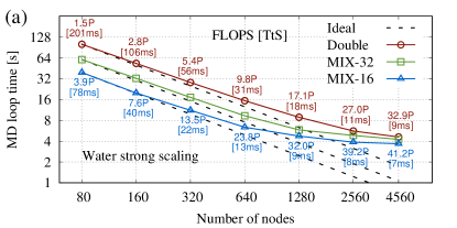
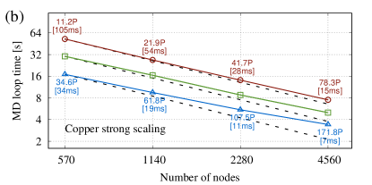
Figure 5: Strong scaling: (a) the water system of 12,779,520 atoms. (b) the copper system of 15,925,248 atoms. The FLOPs of the copper system is 3.9 times compared to that of the water system. The MD loop time is measured using the wall clock time of 500 MD steps (energy and forces are computed 501 times). The corresponding peak performance in PFLOPS and the time-to-solution (TtS) in millisecond per MD step are presented.

VII-B2 Weak scaling

The weak scaling of the optimized DeePMD-kit is measured in terms of the FLOPS of 500 MD steps for both water and copper (Fig. 6). Both systems show perfect scaling with respect to the number of nodes (GPUs) used. The MIX-32 and MIX-16 versions are about $1.7$/1.8 and $2.6$/3.0 times faster compared to the double-precision code for the water/copper system, respectively. For water and copper, the largest system sizes simulated in these tests are 679 and 127 million atoms, respectively, which are more than three orders of magnitude larger compared to the state-of-the-art MD with ab initio accuracy. For the copper system, the peak performance achieved is 91 PFLOPS (45.5% of the peak) in double precision, and 162/275 PFLOPS in MIX-32/MIX-16 precision. The time-to-solution is $8.1/4.6/2.7\times 10^{-10}$ second/step/atom in double/MIX-32/MIX-16 precision, which means that one nanosecond MD simulation of the 127M-atom system with ab initio accuracy can be finished in 29/16/9.5 hours. For the water system, the peak performance is 79.9 PFLOPS (40% of the peak) in double precision, and 138.8/211.5 PFLOPS in MIX-32/MIX-16 precision. The optimized code reaches a time-to-solution of $3.0/1.7/1.1\times 10^{-10}$ second/step/atom in double/MIX-32/MIX-16 precision, so that one nanosecond MD simulation of the 679M-atom water system with ab initio accuracy can be finished in 112/64/42 hours. We remark that the computationally feasible system sizes for MIX-32 and MIX-16 codes on the 4,560 computing nodes of Summit can keep increasing to $1.35$ and $2.7$ billion atoms, respectively, and will be ultimately limited by the capacity of the GPU memory. Moreover, the perfect weak scaling of both systems implies that the optimized DeePMD-kit is able to calculate even bigger physical systems on future exascale supercomputers with no intrinsic obstacles.

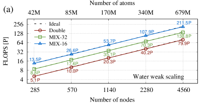
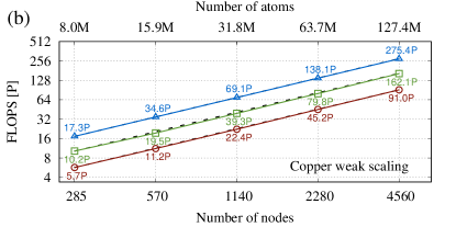
Figure 6: Weak scaling: (a) the water system. Number of atom ranges from 42,467,328 to 679,477,248. (b) the copper system. Number of atoms ranges from 7,962,624 to 127,401,984.

VII-C Sustained performance

The MD loop time of the optimized DeePMD-kit has been measured and discussed in detail in Secs. VII-A and VII-B. By subtracting the MD loop time from the total wall clock time, we define the “setup time”, which mainly includes the initialization of the atomic structure and the loading of the DP model data. In the baseline implementation, the atomic structure is constructed on a single MPI task and then distributed via MPI communication, and the model data is read in from the hard-drive by all the MPI tasks. The corresponding setup time can be a few minutes, though they are performed only once. For example, the setup time for the copper system of $127,401,984$ atoms is more than $263$ seconds on 4,560 computing nodes on Summit.

To reduce these overheads, we build the atomic structure with all the MPI tasks without communication, and the model data is also staged by first reading in with a single MPI rank, and then broadcasting across all MPI tasks. By these optimizations, the setup time is reduced to less than $5$ seconds for all tests. The sustained performance of the DeePMD-kit reaches 90.3 PFLOPS (45% of the peak) in double precision when running the 127,401,984 atoms copper system for 5,000 MD steps (5 ps).

VII-D Network size

The performance of the DeePMD-kit with respect to the matrix size of the last layer of the embedding net is shown in Fig. 7. While the FLOPS curves of both double and MIX-32 versions flatten after the matrix size reaching $256\times 512$, that of the MIX-16 version keeps increasing and reaches $1.17$ EFLOPS when the matrix is of size $1024\times 2048$. This is mainly because half precision arithmetic is only efficient when the matrix size is bigger than $2048\times 2048$ [72]. Although larger FLOPS comes with bigger networks, we notice that it is enough to achieve the ab initio accuracy with matrix size $64\times 128$, and the accuracy improvement by using larger embedding nets is negligible. Therefore, in this paper, we report the performance of the DeePMD-kit based on the matrix size $64\times 128$. In this regime, the performance is mainly dominated by the GPU memory bandwidth, as discussed in section  VII-A. As the size of the embedding net grows to $1024\times 2048$, the GEMM operations takes more than $85\%$ of the GPU computational time in all versions of DeePMD-kit. The computational efficiencies of both double precision and MIX-32 achieve about $90\%$, though that of the half precision only reaches $42\%$, which indicates that the performance of the double and MIX-32 are compute-bound, and the MIX-16 version is still memory-bound. Such performance behavior can be understood by the FLOP/Byte ratio of the V100 GPU, and will be discussed in section  VIII-B. We remark that larger network size may be needed to achieve better accuracy in more complicated physical systems than pure water and copper. In those cases, the MIX-16 scheme is even more favorable in terms of efficiency.

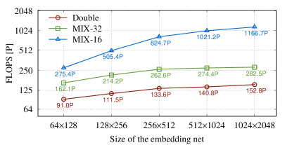
Figure 7: The FLOPS achieved with respect of the size of the embedding net. The FLOPS is measured with the copper system on 4,560 nodes. The size of the embedding net is characterized by the size of the network parameter matrix ${W}$ of the largest hidden layer. The embedding net investigated in this work is 64$\times$128.

VIII Implications

This work provides a vivid demonstration of what can be achieved by integrating physics-based modeling and simulation, machine learning, and efficient implementation on the next-generation computational platform. It opens up a host of new exciting possibilities in applications to material science, chemistry, and biology, as introduced in Sec. VIII-A. It also poses new challenges to the next-generation supercomputer for a better integration of machine learning and physical modeling, as detailed in Sec. VIII-B. We believe that this work may represent a turning point in the history of high-performance computing, and it will have profound implications not only in the field of molecular simulation, but also in other areas of scientific computing.

VIII-A Applications of Optimized DeePMD-kit

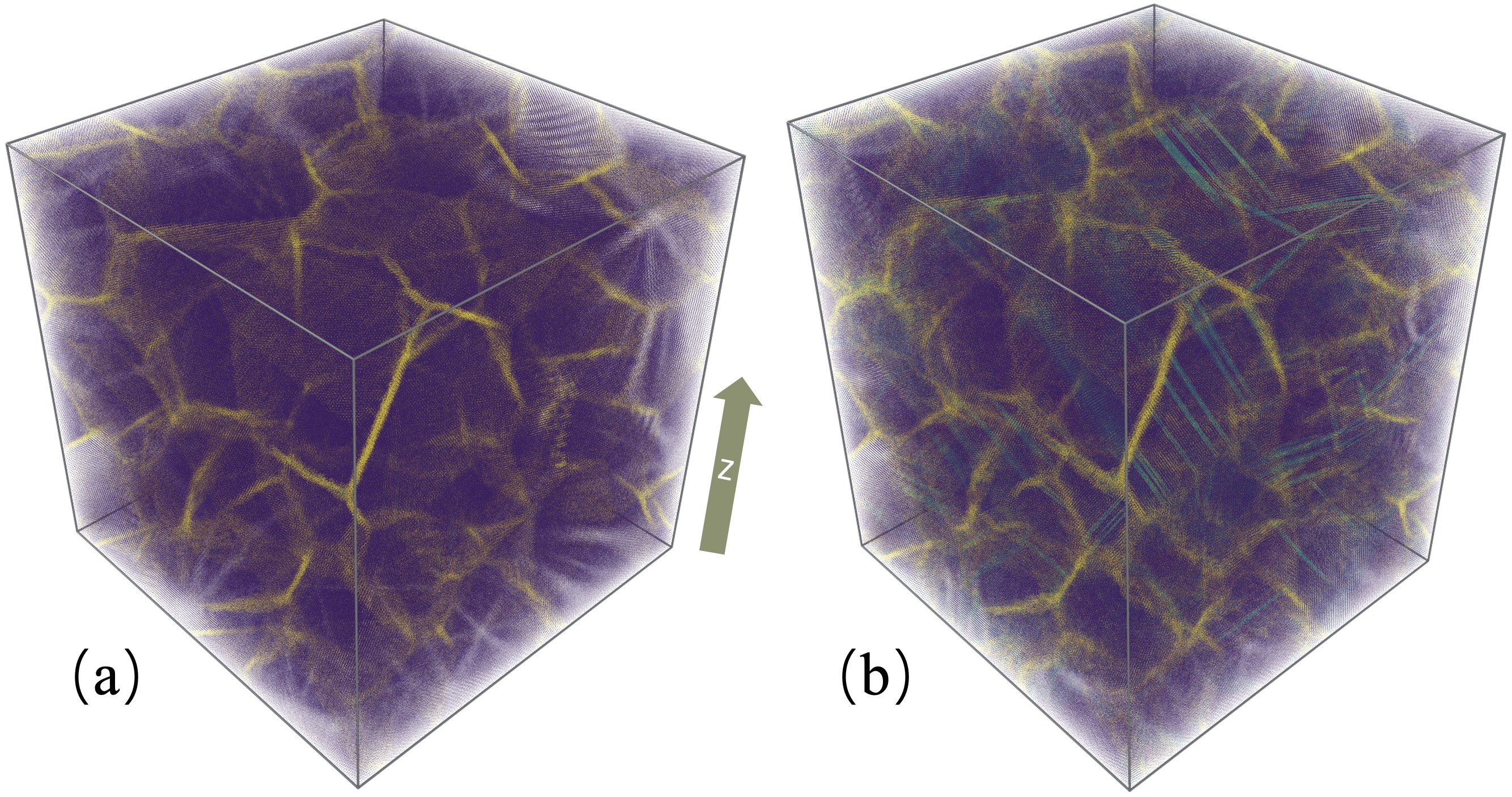
Figure 8: (a) A 10,401,218-atom nanocrystalline copper consisting of 64 randomly oriented crystals with 15-nm averaged grain diameter. (b) The nanocrystalline copper after 10% tensile deformation along the $z$ axis. Purple, yellow, and cyan denote the atoms in the grains, atoms in the grain boundaries, and atoms in the stacking faults.

The strength and hardness of metals can be enhanced by refining their grains, and MD can be of great help to provide microscopic insights into the underlying mechanism [21, 22]. Typically, a nanocrystalline structure of metal consists of tens to hundreds of millions of atoms [21, 22], which is far beyond the capability of ab initio methods. Therefore, previous simulation of nanocrystalline metals can only be driven by EFFs with limited accuracy. Taking copper as an example, EFFs are able to yield the strain-stress curves of nanocrystalline, from which the movements of dislocations and grain boundaries can be analyzed to elucidate the origins of strength in nanocrystalline. However, the biggest problem of EFFs is the lack of accuracy for certain properties, e.g., surface formation energies and stacking fault energies. The accuracy problem is largely resolved by the DP model used in this work. We refer to Ref. [70] for extensive benchmark.

We show in Fig. 8 the tensile deformation of a 10,401,218-atom nanocrystalline copper by MD simulations. The initial cell size is set to $50\times 50\times 50$ nm³. We run 50,000 steps with a time-step of 0.5 fs. The first 10,000 steps are used for annealing at 300 K while the remaining 40,000 steps follow a strain rate of 5$\times$10⁸ s^-1. In total, the nanocrystalline copper is deformed by 10%. We adopt the common neighbor analysis scheme [73, 74] to analyze the structure of nanocrystalline copper. As shown in Fig. 8, the atoms in the grains have a face-centerd cubic (fcc) local structure, which is the ground-state structure of copper. After the deformation, stacking faults of copper are identified by monitoring the formation of hexagonal close-packed (hcp) structures. This example demonstrates the dynamical tensile deformation process of a nanocrystalline copper system. We leave detailed analyses to a future paper that is dedicated to the physics of this process.

Applications enabled by the multi-GPU implementation of the DeePMD-kit code can go far beyond copper and water systems reported here, and can span a wide spectrum of complex materials and molecules. This first stems from the wide applicability of the DP method to problems in different fields. Being a general model based on both machine learning and physics, DP inherits the accuracy from first-principles methods and puts on an equal footing the description of atomic interaction in the cases of bio-molecules, insulators, metals, and semi-metals, etc. This ability of DP is further boosted by this work, which takes advantage of the state-of-the-art supercomputers, and makes simulation of hundreds of millions of atoms with ab initio accuracy a routine procedure. In the short term, this will directly benefit the study of many problems of practical interests, such as complex chemical reactions [18, 19], electrochemical cells [20], nanocrystalline materials [75, 21, 22], irradiation damages [23], and dynamic fracture and crack propagation [24, 25], etc., for which a very high accuracy and a system size of thousands to hundreds of millions of atoms, or even larger, is often required. In a longer term, this could be used to problems of significant practical interest, such as drug design and materials design.

VIII-B Outlook in the era of Exascale computing

The past decade has witnessed the rapid growth of the many-core architecture due to its superior performance in FLOPS per watt and memory bandwidth. This essentially requires a revisit of the scientific applications and a rethinking of the optimal data layout and MPI communication at an algorithmic level, rather than simply offloading computational intensive tasks. In this paper, the critical data layout in DeePMD is redesigned to increase the task granularity, then the entire DeePMD-kit code is parallelized and optimized to improve its scalability and efficiency on the GPU supercomputer Summit. The optimization strategy presented in this paper can also be applied to other many-core architectures. For example, it can be easily converted to the Heterogeneous-compute Interface for Portability (HIP) programming model to run on the next exascale supercomputer Frontier, which will be based on AMD GPUs.

In the pursuit of greater computational power, the computational power v.s. memory bandwidth ratio (or FLOP/Byte ratio in short) rises rapidly, especially when specialized half-precision hardware is involved. For example, the double-precision FLOP/Byte ratio on V100 GPU is 7.8, while the half-precision FLOP/Byte ratio is 133.3 ($120$TFLOPS/$900$GB/s$=133.3$ FLOP/B), which means the 120 TFLOPS half-precision computing power can only be achieved when 133 operations are executed after a single byte is loaded from global memory into the GPU. Such a high ratio makes it difficult to utilize the full computing power of the Tensor Cores with small matrix size, which is exactly in the case of optimized DeePMD-kit — the MIX-16 version is mainly bounded by the GPU memory bandwidth. This implies that future improvement of the FLOP/Byte ratio for the many-core architecture, especially for the half-precision specialized hardware, can benefit HPC+AI applications such as DeePMD-kit. We notice that on the newly announced Fugaku supercomputer, the Fujitsu A64FX CPU has a FLOP/Byte ratio of 13.2 ($13.51$TFLOPS/$1024$GB/s$=13.2$FLOP/Byte) in the boost mode. Therefore, in theory, the optimized DeePMD-kit should achieve better performance on the Fugaku supercomputer. In addition, the computationally feasible system size of the optimized DeePMD-kit can be increased on future many-core architecture if the capacity of the high bandwidth memory is expanded.

Based on the scaling shown in Fig. 6, we see no intrinsic obstacles to scaling our code to run on the exascale supercomputer for systems with billions of atoms. Compared to the traditional numerical methods such as density functional theory, one advantage of Deep Potential lies in its resilience to numerical noise, which could significantly reduce the amount of work needed for fault-tolerant treatments. Therefore, methods like DeePMD can be ideal candidates in the upcoming era of exascale computing. On the other hand, improvements on the hardware, especially reducing the latency of GPU and network, are required to achieve better strong scaling for the DeePMD-kit on the next generation supercomputers.

References

- [1] D. Frenkel and B. Smit, Understanding molecular simulation. Orlando, FL, USA: Academic Press, 2001.
- [2] M. Tuckerman, Statistical mechanics: theory and molecular simulation. Oxford university press, 2010.
- [3] R. Car and M. Parrinello, “Unified approach for molecular dynamics and density-functional theory,” Physical Review Letters, vol. 55, no. 22, p. 2471, 1985.
- [4] D. Marx and J. Hutter, Ab initio molecular dynamics: basic theory and advanced methods. Cambridge University Press, 2009.
- [5] P. Hohenberg and W. Kohn, “Inhomogeneous electron gas,” Physical Review, vol. 136, p. 864B, 1964.
- [6] W. Kohn and L. J. Sham, “Self-consistent equations including exchange and correlation effects,” Physical Review, vol. 140, no. 4A, p. A1133, 1965.
- [7] P. Carloni, U. Rothlisberger, and M. Parrinello, “The role and perspective of ab initio molecular dynamics in the study of biological systems,” Accounts of Chemical Research, vol. 35, no. 6, pp. 455–464, 2002.
- [8] M. Aminpour, C. Montemagno, and J. A. Tuszynski, “An overview of molecular modeling for drug discovery with specific illustrative examples of applications,” Molecules, vol. 24, no. 9, p. 1693, 2019.
- [9] K. Leung and S. B. Rempe, “Ab initio molecular dynamics study of glycine intramolecular proton transfer in water,” The Journal of chemical physics, vol. 122, no. 18, p. 184506, 2005.
- [10] M. Chen, L. Zheng, B. Santra, H.-Y. Ko, R. A. DiStasio Jr, M. L. Klein, R. Car, and X. Wu, “Hydroxide diffuses slower than hydronium in water because its solvated structure inhibits correlated proton transfer,” Nature chemistry, vol. 10, no. 4, pp. 413–419, 2018.
- [11] J.-Y. Raty, F. Gygi, and G. Galli, “Growth of carbon nanotubes on metal nanoparticles: a microscopic mechanism from ab initio molecular dynamics simulations,” Physical review letters, vol. 95, no. 9, p. 096103, 2005.
- [12] F. Gygi, E. W. Draeger, M. Schulz, B. R. De Supinski, J. A. Gunnels, V. Austel, J. C. Sexton, F. Franchetti, S. Kral, C. W. Ueberhuber et al., “Large-scale electronic structure calculations of high-z metals on the bluegene/l platform,” in Proceedings of the 2006 ACM/IEEE conference on Supercomputing. New York, United States: Association for Computing Machinery, 2006, pp. 45–es.
- [13] S. Das, P. Motamarri, V. Gavini, B. Turcksin, Y. W. Li, and B. Leback, “Fast, scalable and accurate finite-element based ab initio calculations using mixed precision computing: 46 pflops simulation of a metallic dislocation system,” in Proceedings of the International Conference for High Performance Computing, Networking, Storage and Analysis. New York, United States: Association for Computing Machinery, 2019, pp. 1–11.
- [14] L.-W. Wang, B. Lee, H. Shan, Z. Zhao, J. Meza, E. Strohmaier, and D. H. Bailey, “Linearly scaling 3d fragment method for large-scale electronic structure calculations,” in SC’08: Proceedings of the 2008 ACM/IEEE Conference on Supercomputing. IEEE, 2008, pp. 1–10.
- [15] M. Eisenbach, C.-G. Zhou, D. M. Nicholson, G. Brown, J. Larkin, and T. C. Schulthess, “A scalable method for ab initio computation of free energies in nanoscale systems,” in Proceedings of the Conference on High Performance Computing Networking, Storage and Analysis. New York, United States: Association for Computing Machinery, 2009, pp. 1–8.
- [16] P. T. Różański and M. Zieliński, “Linear scaling approach for atomistic calculation of excitonic properties of 10-million-atom nanostructures,” Physical Review B, vol. 94, no. 4, p. 045440, 2016.
- [17] A. Nakata, J. Baker, S. Mujahed, J. T. Poulton, S. Arapan, J. Lin, Z. Raza, S. Yadav, L. Truflandier, T. Miyazaki et al., “Large scale and linear scaling dft with the conquest code,” arXiv preprint arXiv:2002.07704, 2020.
- [18] A. Nakano, R. K. Kalia, K.-i. Nomura, A. Sharma, P. Vashishta, F. Shimojo, A. C. van Duin, W. A. Goddard, R. Biswas, and D. Srivastava, “A divide-and-conquer/cellular-decomposition framework for million-to-billion atom simulations of chemical reactions,” Computational Materials Science, vol. 38, no. 4, pp. 642–652, 2007.
- [19] X. Li, Z. Mo, J. Liu, and L. Guo, “Revealing chemical reactions of coal pyrolysis with gpu-enabled reaxff molecular dynamics and cheminformatics analysis,” Molecular Simulation, vol. 41, no. 1-3, pp. 13–27, 2015.
- [20] R. Jorn, R. Kumar, D. P. Abraham, and G. A. Voth, “Atomistic modeling of the electrode–electrolyte interface in li-ion energy storage systems: electrolyte structuring,” The Journal of Physical Chemistry C, vol. 117, no. 8, pp. 3747–3761, 2013.
- [21] J. Schiøtz, F. D. Di Tolla, and K. W. Jacobsen, “Softening of nanocrystalline metals at very small grain sizes,” Nature, vol. 391, no. 6667, pp. 561–563, 1998.
- [22] J. Schiøtz and K. W. Jacobsen, “A maximum in the strength of nanocrystalline copper,” Science, vol. 301, no. 5638, pp. 1357–1359, 2003.
- [23] F. Gao and W. J. Weber, “Atomic-scale simulation of 50 kev si displacement cascades in -sic,” Physical Review B, vol. 63, no. 5, p. 054101, 2000.
- [24] P. Vashishta, A. Nakano, R. K. Kalia, and I. Ebbsjö, “Crack propagation and fracture in ceramic films—million atom molecular dynamics simulations on parallel computers,” Materials Science and Engineering: B, vol. 37, no. 1-3, pp. 56–71, 1996.
- [25] P. Vashishta, R. K. Kalia, and A. Nakano, “Large-scale atomistic simulations of dynamic fracture,” Computing in science & engineering, vol. 1, no. 5, pp. 56–65, 1999.
- [26] A. Laio and M. Parrinello, “Escaping free-energy minima,” Proceedings of the National Academy of Sciences, vol. 99, no. 20, pp. 12 562–12 566, 2002.
- [27] L. Zhang, H. Wang, and W. E, “Reinforced dynamics for enhanced sampling in large atomic and molecular systems,” The Journal of Chemical Physics, vol. 148, no. 12, p. 124113, 2018.
- [28] G. D. Purvis III and R. J. Bartlett, “A full coupled-cluster singles and doubles model: The inclusion of disconnected triples,” The Journal of Chemical Physics, vol. 76, no. 4, pp. 1910–1918, 1982.
- [29] A. C. Van Duin, S. Dasgupta, F. Lorant, and W. A. Goddard, “Reaxff: a reactive force field for hydrocarbons,” The Journal of Physical Chemistry A, vol. 105, no. 41, pp. 9396–9409, 2001.
- [30] J. Wang, R. M. Wolf, J. W. Caldwell, P. A. Kollman, and D. A. Case, “Development and testing of a general amber force field,” Journal of computational chemistry, vol. 25, no. 9, pp. 1157–1174, 2004.
- [31] B. R. Brooks, C. L. Brooks III, A. D. Mackerell Jr, L. Nilsson, R. J. Petrella, B. Roux, Y. Won, G. Archontis, C. Bartels, S. Boresch et al., “Charmm: the biomolecular simulation program,” Journal of computational chemistry, vol. 30, no. 10, pp. 1545–1614, 2009.
- [32] B. Jelinek, S. Groh, M. F. Horstemeyer, J. Houze, S.-G. Kim, G. J. Wagner, A. Moitra, and M. I. Baskes, “Modified embedded atom method potential for al, si, mg, cu, and fe alloys,” Physical Review B, vol. 85, no. 24, p. 245102, 2012.
- [33] T. P. Senftle, S. Hong, M. M. Islam, S. B. Kylasa, Y. Zheng, Y. K. Shin, C. Junkermeier, R. Engel-Herbert, M. J. Janik, H. M. Aktulga et al., “The reaxff reactive force-field: development, applications and future directions,” npj Computational Materials, vol. 2, no. 1, pp. 1–14, 2016.
- [34] J. Behler and M. Parrinello, “Generalized neural-network representation of high-dimensional potential-energy surfaces,” Physical Review Letters, vol. 98, no. 14, p. 146401, 2007.
- [35] A. P. Bartók, M. C. Payne, R. Kondor, and G. Csányi, “Gaussian approximation potentials: The accuracy of quantum mechanics, without the electrons,” Physical Review Letters, vol. 104, no. 13, p. 136403, 2010.
- [36] S. Chmiela, A. Tkatchenko, H. E. Sauceda, I. Poltavsky, K. T. Schütt, and K.-R. Müller, “Machine learning of accurate energy-conserving molecular force fields,” Science Advances, vol. 3, no. 5, p. e1603015, 2017.
- [37] K. Schütt, P.-J. Kindermans, H. E. S. Felix, S. Chmiela, A. Tkatchenko, and K.-R. Müller, “Schnet: A continuous-filter convolutional neural network for modeling quantum interactions,” in Advances in Neural Information Processing Systems, 2017, pp. 992–1002.
- [38] J. S. Smith, O. Isayev, and A. E. Roitberg, “ANI-1: an extensible neural network potential with dft accuracy at force field computational cost,” Chemical Science, vol. 8, no. 4, pp. 3192–3203, 2017.
- [39] J. Han, L. Zhang, R. Car, and W. E, “Deep potential: a general representation of a many-body potential energy surface,” Communications in Computational Physics, vol. 23, no. 3, pp. 629–639, 2018.
- [40] L. Zhang, J. Han, H. Wang, R. Car, and W. E, “Deep potential molecular dynamics: A scalable model with the accuracy of quantum mechanics,” Physical Review Letters, vol. 120, p. 143001, Apr 2018.
- [41] L. Zhang, J. Han, H. Wang, W. Saidi, R. Car, and W. E, “End-to-end symmetry preserving inter-atomic potential energy model for finite and extended systems,” in Advances in Neural Information Processing Systems 31, S. Bengio, H. Wallach, H. Larochelle, K. Grauman, N. Cesa-Bianchi, and R. Garnett, Eds. Curran Associates, Inc., 2018, pp. 4441–4451.
- [42] A. R. Barron, “Universal approximation bounds for superpositions of a sigmoidal function,” IEEE Transactions on Information theory, vol. 39, no. 3, pp. 930–945, 1993.
- [43] C. Ma, L. Wu, and W. E, “Machine learning from a continuous viewpoint,” arXiv preprint arXiv:1912.12777, 2019.
- [44] L. Zhang, D.-Y. Lin, H. Wang, R. Car, and W. E, “Active learning of uniformly accurate interatomic potentials for materials simulation,” Physical Review Materials, vol. 3, no. 2, p. 023804, 2019.
- [45] H. Wang, L. Zhang, J. Han, and W. E, “DeePMD-kit: A deep learning package for many-body potential energy representation and molecular dynamics,” Computer Physics Communications, vol. 228, pp. 178–184, 2018.
- [46] Y. Hasegawa, J.-I. Iwata, M. Tsuji, D. Takahashi, A. Oshiyama, K. Minami, T. Boku, F. Shoji, A. Uno, M. Kurokawa et al., “First-principles calculations of electron states of a silicon nanowire with 100,000 atoms on the k computer,” in Proceedings of 2011 International Conference for High Performance Computing, Networking, Storage and Analysis. New York, United States: Association for Computing Machinery, 2011, pp. 1–11.
- [47] K. Lee, D. Yoo, W. Jeong, and S. Han, “Simple-nn: An efficient package for training and executing neural-network interatomic potentials,” Computer Physics Communications, vol. 242, pp. 95–103, 2019.
- [48] A. Singraber, J. Behler, and C. Dellago, “Library-based lammps implementation of high-dimensional neural network potentials,” Journal of chemical theory and computation, vol. 15, no. 3, pp. 1827–1840, 2019.
- [49] M. F. Calegari Andrade, H.-Y. Ko, L. Zhang, R. Car, and A. Selloni, “Free energy of proton transfer at the water–tio2 interface from ab initio deep potential molecular dynamics,” Chem. Sci., vol. 11, pp. 2335–2341, 2020. [Online]. Available: http://dx.doi.org/10.1039/C9SC05116C
- [50] J. Zeng, L. Cao, M. Xu, T. Zhu, and J. Z. Zhang, “Neural network based in silico simulation of combustion reactions,” arXiv preprint arXiv:1911.12252, 2019.
- [51] W.-K. Chen, X.-Y. Liu, W.-H. Fang, P. O. Dral, and G. Cui, “Deep learning for nonadiabatic excited-state dynamics,” The journal of physical chemistry letters, vol. 9, no. 23, pp. 6702–6708, 2018.
- [52] L. Zhang, M. Chen, X. Wu, H. Wang, W. E, and R. Car, “Deep neural network for the dielectric response of insulators,” Phys. Rev. B, vol. 102, p. 041121, Jul 2020. [Online]. Available: https://link.aps.org/doi/10.1103/PhysRevB.102.041121
- [53] H.-Y. Ko, L. Zhang, B. Santra, H. Wang, W. E, R. A. DiStasio Jr, and R. Car, “Isotope effects in liquid water via deep potential molecular dynamics,” Molecular Physics, vol. 117, no. 22, pp. 3269–3281, 2019.
- [54] F.-Z. Dai, B. Wen, Y. Sun, H. Xiang, and Y. Zhou, “Theoretical prediction on thermal and mechanical properties of high entropy (zr0. 2hf0. 2ti0. 2nb0. 2ta0. 2) c by deep learning potential,” Journal of Materials Science & Technology, vol. 43, pp. 168–174, 2020.
- [55] A. Marcolongo, T. Binninger, F. Zipoli, and T. Laino, “Simulating diffusion properties of solid-state electrolytes via a neural network potential: Performance and training scheme,” ChemSystemsChem, vol. 2, p. e1900031, 2019.
- [56] H. Wang, X. Guo, L. Zhang, H. Wang, and J. Xue, “Deep learning inter-atomic potential model for accurate irradiation damage simulations,” Applied Physics Letters, vol. 114, no. 24, p. 244101, 2019.
- [57] Q. Liu, D. Lu, and M. Chen, “Structure and dynamics of warm dense aluminum: A molecular dynamics study with density functional theory and deep potential,” Journal of Physics: Condensed Matter, vol. 32, no. 14, p. 144002, 2020.
- [58] L. Bourgeois, Y. Zhang, Z. Zhang, Y. Chen, and N. V. Medhekar, “Transforming solid-state precipitates via excess vacancies,” Nature communications, vol. 11, no. 1, pp. 1–10, 2020.
- [59] H. Niu, L. Bonati, P. M. Piaggi, and M. Parrinello, “Ab initio phase diagram and nucleation of gallium,” Nature Communications, vol. 11, no. 1, pp. 1–9, 2020.
- [60] A. P. Bartók, R. Kondor, and G. Csányi, “On representing chemical environments,” Physical Review B, vol. 87, no. 18, p. 184115, 2013.
- [61] “Quantum mechanics and interatomic potentials,” https://github.com/libAtoms/QUIP, Accessed: 2020-03-03.
- [62] A. Khorshidi and A. A. Peterson, “Amp: A modular approach to machine learning in atomistic simulations,” Computer Physics Communications, vol. 207, pp. 310–324, 2016.
- [63] K. Yao, J. E. Herr, D. W. Toth, R. Mckintyre, and J. Parkhill, “The tensormol-0.1 model chemistry: a neural network augmented with long-range physics,” Chemical science, vol. 9, no. 8, pp. 2261–2269, 2018.
- [64] A. S. Abbott, J. M. Turney, B. Zhang, D. G. Smith, D. Altarawy, and H. F. Schaefer, “Pes-learn: An open-source software package for the automated generation of machine learning models of molecular potential energy surfaces,” Journal of Chemical Theory and Computation, vol. 15, no. 8, pp. 4386–4398, 2019.
- [65] S. Plimpton, “Fast parallel algorithms for short-range molecular dynamics,” Journal of Computational Physics, vol. 117, no. 1, pp. 1–19, 1995.
- [66] M. Abadi, P. Barham, J. Chen, Z. Chen, A. Davis, J. Dean, M. Devin, S. Ghemawat, G. Irving, M. Isard, M. Kudlur, J. Levenberg, R. Monga, S. Moore, D. G. Murray, B. Steiner, P. Tucker, V. Vasudevan, P. Warden, M. Wicke, Y. Yu, and X. Zheng, “Tensorflow: A system for large-scale machine learning,” in 12th USENIX Symposium on Operating Systems Design and Implementation (OSDI 16). Savannah, GA: USENIX Association, Nov. 2016, pp. 265–283. [Online]. Available: https://www.usenix.org/conference/osdi16/technical-sessions/presentation/abadi
- [67] R. A. DiStasio Jr., B. Santra, Z. Li, X. Wu, and R. Car, “The individual and collective effects of exact exchange and dispersion interactions on the ab initio structure of liquid water,” J. Chem. Phys., vol. 141, p. 084502, Aug. 2014.
- [68] M. Chen, H.-Y. Ko, R. C. Remsing, M. F. C. Andrade, B. Santra, Z. Sun, A. Selloni, R. Car, M. L. Klein, J. P. Perdew, and X. Wu, “Ab initio theory and modeling of water,” Proc. Natl. Acad. Sci. U.S.A., vol. 114, pp. 10 846–10 851, Sep. 2017.
- [69] G. M. Sommers, M. F. Calegari Andrade, L. Zhang, H. Wang, and R. Car, “Raman spectrum and polarizability of liquid water from deep neural networks,” Phys. Chem. Chem. Phys., vol. 22, pp. 10 592–10 602, 2020. [Online]. Available: http://dx.doi.org/10.1039/D0CP01893G
- [70] Y. Zhang, H. Wang, W. Chen, J. Zeng, L. Zhang, H. Wang, and W. E, “Dp-gen: A concurrent learning platform for the generation of reliable deep learning based potential energy models,” Computer Physics Communications, p. 107206, 2020.
- [71] https://www.top500.org, June 2020 (accessed 2020-08-01).
- [72] S. Markidis, S. W. Der Chien, E. Laure, I. B. Peng, and J. S. Vetter, “Nvidia tensor core programmability, performance & precision,” in 2018 IEEE International Parallel and Distributed Processing Symposium Workshops (IPDPSW). IEEE, 2018, pp. 522–531.
- [73] H. Jónsson and H. C. Andersen, “Icosahedral ordering in the lennard-jones liquid and glass,” Physical review letters, vol. 60, no. 22, p. 2295, 1988.
- [74] A. S. Clarke and H. Jónsson, “Structural changes accompanying densification of random hard-sphere packings,” Phys. Rev. E, vol. 47, pp. 3975–3984, Jun 1993. [Online]. Available: https://link.aps.org/doi/10.1103/PhysRevE.47.3975
- [75] A. C. Lund, T. Nieh, and C. Schuh, “Tension/compression strength asymmetry in a simulated nanocrystalline metal,” Physical Review B, vol. 69, no. 1, p. 012101, 2004.