Topological delocalization in the completely disordered two-dimensional quantum walk

Abstract

We investigate numerically and theoretically the effect of spatial disorder on two-dimensional split-step discrete-time quantum walks with two internal “coin” states. Spatial disorder can lead to Anderson localization, inhibiting the spread of quantum walks, putting them at a disadvantage against their diffusively spreading classical counterparts. We find that spatial disorder of the most general type, i.e., position-dependent Haar random coin operators, does not lead to Anderson localization, but to a diffusive spread instead. This is a delocalization, which happens because disorder places the quantum walk to a critical point between different anomalous Floquet-Anderson insulating topological phases. We base this explanation on the relationship of this general quantum walk to a simpler case more studied in the literature, and for which disorder-induced delocalization of a topological origin has been observed. We review topological delocalization for the simpler quantum walk, using time-evolution of the wavefunctions and level spacing statistics. We apply scattering theory to two-dimensional quantum walks, and thus calculate the topological invariants of disordered quantum walks, substantiating the topological interpretation of the delocalization, and finding signatures of the delocalization in the finite-size scaling of transmission. We show criticality of the Haar random quantum walk by calculating the critical exponent $\eta$ in three different ways, and find $\eta\approx 0.52$ as in the integer quantum Hall effect. Our results showcase how theoretical ideas and numerical tools from solid-state physics can help us understand spatially random quantum walks.

I Introduction

Discrete-Time Quantum Walks (or quantum walks for short) are the quantum generalizations of random walks Kempe (2003); Genske et al. (2013). They are promising components of quantum algorithms because they spread faster than their classical counterparts Ambainis et al. (2020). These quantum walks can be described as periodic sequences of unitary “coin toss” and “shift” operations applied to a particle on a lattice. If the particle is initially on one of the lattice sites, during the quantum walk, its wavefunction spreads out over the lattice to infinity in a ballistic way, i.e., with root-mean-square distance from the origin proportional to time elapsed. This is faster than the diffusive spread characteristic of classical random walks.

Spatial disorder in the quantum walk parameters can be detrimental to the fast spread of the walk. Intuition from solid-state physics suggest that the combination of disorder and coherence generically leads to Anderson localization Nagaoka (1985): all eigenstates assume an exponentially localized envelope). As a consequence, a particle starting from a single site cannot spread off to infinity, its wavefunction remains within a bounded region, to exponential accuracy. Anderson localization can be tested numerically from the spectrum of the Hamiltonian, alternatively from the conductance, or from the spreading of the wavefunction Sepehrinia and Sheikhan (2011). Anderson localization indeed happens in quantum walks Joye (2012); Vakulchyk et al. (2017), and has already been observed in experiment Schreiber et al. (2011); Pankov et al. (2019). We note this is very different than the dynamical effect of fluctuating disorder: that, by inducing a loss of coherence, would lead to diffusive spreading, i.e., a loss of the “quantum advantage”Dür et al. (2002); Schreiber et al. (2011). This is also different from the so-called trapping effect in quantum walks Kollár et al. (2015); Machida and Chandrashekar (2015); Kollár et al. (2020), which is a form of localization without disorder, related to the presence of flat bands in the quasienergy spectrum.

Another interesting feature of quantum walks is that they can have topological phases, of the kind known from the physics of topological insulators and superconductors Hasan and Kane (2010); Kitagawa et al. (2010); Tarasinski et al. (2014); Cedzich et al. (2018). On one hand, this allows quantum walks to be used as simulators for these solid state physics systems. On the other hand, quantum walks also have topological phases beyond those of topological insulators, which are prototypical of periodically driven, Floquet systems Rudner et al. (2013); Asbóth and Edge (2015). Thus, they can be used as versatile toy models for periodically driven systems in the nonperturbative limit of strong driving.

Recently, a striking disorder-induced delocalization phenomenon was observed for the simplest two-dimensional quantum walk Edge and Asbóth (2015), related to its topological phases. This quantum walk is the split-step walk on a square lattice, with two internal (coin) states, and a real-valued coin operator. Disorder, added to the walk via an onsite complex phase factor (mimicking onsite potential disorder), leads to an anomalous Floquet-Anderson insulator (AFAI) state Titum et al. (2016), with Anderson localization of all bulk eigenstates yet with topologically protected edge states present in the spectrum. If the coin operator is finetuned to a critical value at the transition between two topological insulating phases, disorder does not lead to Anderson localization, but rather to a diffusive spread Edge and Asbóth (2015). This route to delocalization also explains the lack of Anderson localization observed elsewhere for some two-dimensional walks Zeng and Yong (2017). Intriguingly, this delocalization can also be achieved if instead of fine tuning the coin operator parameters, they are chosen to be maximally disordered Edge and Asbóth (2015). This happens because coin disorder can tune the bulk topological invariant and hence also put the system to a critical point—an example is the case where the coin rotation angle is uniformly random. We note that this localization-delocalization transition has a completely different physical origin than that induced by correlated disorder Mendes et al. (2019). It is also different from delocalization in one-dimensional quantum walks Obuse and Kawakami (2011); Zhao and Gong (2015); Rakovszky and Asbóth (2015) in that it does not require chiral symmetry.

In this article we ask whether we see Anderson localization or topological delocalization in the completely disordered (Haar random) general two-state quantum walk on the square lattice, where the coin is picked from all $U(2)$ operators in a Haar uniform random way. We employ a numerical tool used in previous work Edge and Asbóth (2015), namely, time evolution of the wavefunction, which is more efficient to compute for quantum walks than for static Hamiltonians. We also use other numerical tools, which have been applied to quantum walks less often: (1) analysis of the level spacing distribution to help identify Anderson localization and (2) calculation of the transmission matrix both to calculate the topological invariants with disorder and to find signatures in the finite-size scaling of Anderson localization and diffusion. We make use of the fact that when there is a complete phase disorder—as in the case when coin operators are Haar uniformly random—all properties of the spectrum should be quasienergy independent, and thus disorder averaging can be replaced/supplemented by quasienergy averaging, which results in a substantial numerical advantage. We find that the completely disordered (Haar random) two-dimensional quantum walk is topologically delocalized, for a similar reason as the more restricted quantum walk.

Our article is organized as follows. In Sec. II we introduce the split-step two-dimensional quantum walk with two internal states and discuss the topological properties in the clean, translational invariant setting. In Sec. III we introduce the scattering matrix of the quantum walk and use it to calculate the topological invariants in the case with disorder. In Sec. IV we compute time evolution, the level spacing statistics, and the finite-size scaling of the transmission, to show that disorder in the phase parameter leads to Anderson localization, except if the system is in a critical state. In Sec. V we show using the numerical tools mentioned above that turning the disorder to the “most random” case, i.e., coin operator from Haar uniform random distribution, leads to delocalization. In Sec. VI we calculate the critical exponent $\eta$ of the Haar random quantum walk in three different ways: autocorrelation of the position distribution, fractal analysis of position distribution, and time dependence of the position distribution peak at the origin. We conclude in Sec. VII and show some preliminary investigation of the case of binary disorder in the coin angle parameter $\theta$ in Appendix.

II Two-dimensional quantum walk with two internal states

The quantum walk we consider in this paper is the time evolution of a particle with two internal (spin) states on a square lattice. Its wavefunction reads,

$$|{\Psi(t)}\rangle =\sum_{x}\sum_{y}\sum_{s=\pm 1}\Psi_{x,y,s}(t)|{x,y,s}\rangle,$$ (1)

where $x,y\in\mathbb{Z}$ are lattice coordinates and we are interested in the state at discrete times $t\in\mathbb{N}$. The dynamics is given by a periodic sequence of internal rotations (coin operator) and spin-dependent displacements (shift operator) on the lattice.

The internal rotations are general $U(2)$ operations acting on the internal degree of freedom, in a position-dependent way. We split off a position-dependent phase operator,

$$\hat{F} =\sum_{x,y}\sum_{s=\pm 1}e^{i\phi(x,y)}|{x,y,s}\rangle\langle{x,y,s}|,$$ (2)

and $\hat{R}_{j}$ denotes the remaining SU(2) rotation operator,

$$\hat{R}_{j} =\sum_{x,y}|{x,y}\rangle\langle{x,y}|\otimes\hat{R}\left(\alpha_{j}(x,y),\beta_{j}(x,y),\theta_{j}(x,y)\right),$$ (3)

where $j$ is used to differentiate between different rotations, and

$$R(\alpha,\beta,\theta) =\begin{pmatrix}e^{-i(\alpha+\beta)}\cos\theta&-e^{i(\alpha-\beta)}\sin\theta\\ e^{-i(\alpha-\beta)}\sin\theta&e^{i(\alpha+\beta)}\cos\theta\end{pmatrix}.$$ (4)

Note that this can be written succinctly in Euler angle representation as $\hat{R}=e^{-i\beta\hat{\sigma}_{z}}e^{-i\theta\hat{\sigma}_{y}}e^{-i\alpha\hat{\sigma}_{z}}$, where $\alpha$, $\theta$, and $\beta$, respectively, are the first, second and third Euler angles. Setting $\alpha=\beta=0$ reduces this coin operator to that used in several quantum walk papers Kitagawa et al. (2010); Kitagawa (2012); Edge and Asbóth (2015).

The shifts are spin-dependent translations on the lattice,

$$\hat{S}_{x} =\sum_{x,y}\sum_{s=\pm 1}|{x+s,y}\rangle\langle{x,y}|\otimes|{s}\rangle\langle{s}|;$$ (5a)

$$\hat{S}_{y} =\sum_{x,y}\sum_{s=\pm 1}|{x,y+s}\rangle\langle{x,y}|\otimes|{s}\rangle\langle{s}|.$$ (5b)

The wavefunction of the walk after $t\in\mathbb{N}$ timesteps reads

$$|{\Psi(t)}\rangle =\hat{U}^{t}|{\Psi(0)}\rangle,$$ (6)

where the timestep operator, $\hat{U}$ represents the effect of one period of the quantum walk,

$$\hat{U} =\hat{F}\hat{S}_{y}\hat{R}_{2}\hat{S}_{x}\hat{R}_{1}.$$ (7)

As initial state we took $|{\Psi(0}\rangle=|{x=0,y=0,s=+1}\rangle$—due to the disorder, the internal state of the initial condition plays no role in the time evolution, so any choice of initial state will give qualitatively the same results The parameters of the timestep operator are the position-dependent angle variables: a phase $\phi(x,y)$, and the rotation parameters $\theta_{1,2}(x,y)$, $\alpha_{1,2}(x,y)$, $\beta_{1,2}(x,y)$. In the formulas that follow we will often suppress the explicit position and spin dependence for better readability.

II.1 Sublattice symmetry of the quantum walk

The two-dimensional quantum walk we consider here has a sublattice structure. There are four sublattices on the square lattice of $x,y\in\mathbb{Z}$, according to whether $x$ and $y$ are even ($e$) or odd ($o$), with corresponding projectors defined as, e.g.,

$$\hat{\Pi}_{e,o}=\sum_{x=\text{ even}}\sum_{y=\text{ odd}}|{x,y}\rangle\langle{x,y}|,$$ (8)

with $\hat{\Pi}_{o,e}$, $\hat{\Pi}_{o,o}$, and $\hat{\Pi}_{e,e}$ defined similarly. Since the quantum walk we consider has one shift along both $x$ and $y$ in every timestep, $\hat{U}$ switches sublattices, according to $(e,e)\leftrightarrow(o,o)$ and $(e,o)\leftrightarrow(o,e)$. Therefore, a quantum walk started from one of the 4 sublattices never interferes with a walk started from any other sublattice—assuming that boundary conditions also respect the sublattice structure, e.g., are periodic with both $L_{x}$ and $L_{y}$ even. (We will later also use absorbing boundary conditions, which always respect the sublattice structure independent of system size.)

The sublattice structure has important consequences for the spectrum of $\hat{U}$, which can be appreciated by first considering the spectrum of $\hat{U}^{2}$. The operator $\hat{U}^{2}$ is block diagonal in the sublattice basis, i.e.,

$$\hat{U}^{2}=\sum_{j=e,o}\sum_{l=e,o}\hat{\Pi}_{j,l}\hat{U}^{2}\hat{\Pi}_{j,l}.$$ (9)

Take an eigenstate $|{\Psi}\rangle$ of $\hat{U}^{2}$ on the $(e,e)$ sublattice,

$$\hat{U}^{2}|{\Psi}\rangle =e^{-2i\varepsilon}|{\Psi}\rangle,$$ (10)

with $0\leq\varepsilon<\pi$. First, note that $\hat{U}|{\Psi}\rangle$ is on the $(o,o)$ sublattice, and is an eigenstate of $\hat{U}^{2}$ with the same eigenvalue $e^{-2i\varepsilon}$. Second, we can use $|{\Psi}\rangle$ to generate two eigenstates of $\hat{U}$, since

$$\hat{U} \left(|{\Psi}\rangle\pm e^{i\varepsilon}\hat{U}|{\Psi}\rangle\right)=\pm e^{-i\varepsilon}\left(|{\Psi}\rangle\pm e^{i\varepsilon}\hat{U}|{\Psi}\rangle\right).$$ (11)

These relations also hold for an eigenstate $|{\Psi^{\prime}}\rangle$ on the $(e,o)$ sublattice, with $\hat{U}|{\Psi^{\prime}}\rangle$ on the $(o,e)$ sublattice.

The results of the previous paragraph can be rephrased Asbóth and Edge (2015) as sublattice symmetry of $\hat{U}$, represented by a unitary and Hermitian sublattice operator,

$$\hat{\Gamma}\hat{U}\hat{\Gamma} =-\hat{U},\,\,\text{with} \hat{\Gamma} =\hat{\Pi}_{e,e}+\hat{\Pi}_{e,o}-\hat{\Pi}_{o,o}-\hat{\Pi}_{o,e}.$$ (12)

Every eigenstate $|{\Phi}\rangle$ of the walk has a sublattice symmetric partner,

$$\hat{U}|{\Phi}\rangle =e^{-i\varepsilon}|{\Phi}\rangle\quad\Rightarrow\quad\hat{U}\hat{\Gamma}|{\Phi}\rangle =e^{-i(\varepsilon+\pi)}\hat{\Gamma}|{\Phi}\rangle,$$ (13)

which is related to Eq. (11) by $|{\Phi}\rangle=(|{\Psi}\rangle+e^{i\varepsilon}\hat{U}|{\Psi}\rangle)/\sqrt{2}$.

The sublattice symmetry we defined above is not the same as the sublattice symmetry familiar from solid state physics, which is also known as chiral symmetry. Chiral symmetry states $\hat{\Gamma}\hat{H}\hat{\Gamma}=-\hat{H}$, linking eigenstates of a Hamiltonian at energy $\varepsilon$ to eigenstates at $-\varepsilon$. The quantum walk we consider here has chiral symmetry only if the parameters are finetuned. For chiral symmetry, we need $\phi=0$, and $\alpha_{2}(x,y)=\beta_{1}(x,y)$ and $\alpha_{1}(x,y)=\beta_{2}(x,y)$, moreover, either $\theta_{1}(x,y)=\theta_{2}(x,y)+n\pi$ (with chiral symmetry by $\hat{\sigma}_{x}$), or $\theta_{1}(x,y)=-\theta_{2}(x,y)+n\pi$ (with chiral symmetry by $\hat{\sigma}_{y}$).

II.2 Parameters $\alpha$ and $\beta$ represent a vector potential

The parameters $\alpha_{1,2}(x,y)$ and $\beta_{1,2}(x,y)$ of the coin rotations can be understood to represent a vector potential Yalçınkaya and Gedik (2015); Arnault and Debbasch (2016); Sajid et al. (2019); Cedzich et al. (2019); Mallick (2018). This is best seen by writing the time-step operator in a different timeframe Asbóth and Obuse (2013), which amounts to a similarity transformation on the original time-step operator of Eq. (7):

$$\hat{U}_{2} =e^{-i\alpha_{1}\hat{\sigma}_{z}}\hat{U}e^{i\alpha_{1}\hat{\sigma}_{z}}=e^{-i\phi}\hat{S}_{y}^{\prime}e^{-i\theta_{2}\hat{\sigma}_{y}}\hat{S}_{x}^{\prime}e^{-i\theta_{1}\hat{\sigma}_{y}};$$ (14)

$$\hat{S}_{y}^{\prime} =e^{-i\alpha_{1}\hat{\sigma}_{z}}\hat{S}_{y}e^{-i\beta_{2}\hat{\sigma}_{z}};\quad\hat{S}_{x}^{\prime}=e^{-i\alpha_{2}\hat{\sigma}_{z}}\hat{S}_{x}e^{-i\beta_{1}\hat{\sigma}_{z}}.$$ (15)

First, if $\alpha_{1,2}$ and $\beta_{1,2}$ are independent of position, then their effect on the quantum walk is just a gauge transformation. To prove this, we rewrite Eq. (15) as

$$\hat{S}_{x}^{\prime} =e^{-i(\beta_{1}+\alpha_{2})\hat{x}}\hat{S}_{x}e^{i(\beta_{1}+\alpha_{2})\hat{x}},$$ (16)

where $\hat{x}$ = $\sum_{x}x|{x}\rangle\langle{x}|$ is the position operator corresponding to position coordinate $x$. Thus $\hat{S}^{\prime}_{x}$ is a unitary transformed version of $\hat{S}_{x}$, and the transforming operator commutes with rotations, phase operations, and $\hat{S}_{y}$ as well. Similar statements hold for $\hat{S}^{\prime}_{y}$. Thus, in this case, the timestep operator $\hat{U}_{2}$ of a quantum walk is unitary equivalent to the timestep operator of the same walk with $\alpha_{1,2}=\beta_{1,2}=0$.

For $\alpha_{1,2}(x,y)$ and $\beta_{1,2}(x,y)$ depending on position, we find a more complicated situation. For this more general case, it is helpful to think of the quantum walk as a nearest-neighbor hopping model on the square lattice with time-dependent hopping amplitudes Asbóth and Edge (2015). The angles $\alpha_{1,2}(x,y)$ and $\beta_{1,2}(x,y)$ can then be included in this hopping model by the use of Peierls phases: For a link from site $(x,y)$ to $(x\pm 1,y)$, the corresponding Peierls phase is $\pm(\beta_{1}(x,y)+\alpha_{2}(x\pm 1,y))$, and from $(x,y)$ to $(x,y\pm 1)$, it is $\pm(\beta_{2}(x,y)+\alpha_{1}(x,y\pm 1))$. A caveat: These Peierls phases depend on the sublattice.

II.3 The quantum walk is topological

The quantum walk we consider has topological phases and associated chiral edge states similar to the simpler two-dimensional quantum walk. That simpler quantum walk (i.e., the vector-potential-like parameters $\alpha=\beta=0$), without spatial disorder has been recognized to host robust edge states, even though the Chern numbers of both of its quasienergy bands vanish Kitagawa (2012). The bulk topological invariant explaining the presence of the edge states is a winding number, the RLBL-invariant Rudner et al. (2013); Asbóth and Edge (2015); Asbóth and Alberti (2017); Sajid et al. (2019) we will call $\nu$. Since spatially constant vector-potential-like parameters $\alpha,\beta$ can be gauged away, we can conclude that our quantum walk has a winding number that depends only on the values of $\theta_{1}$ and $\theta_{2}$. The invariant follows a harlequin pattern Asbóth and Edge (2015), which can be put in a concise (although somewhat obfuscated) formula,

$$\nu =\text{sgn}\left[\sin(\theta_{1}-\theta_{2})\sin(\theta_{1}+\theta_{2})\right],$$ (17)

with $\nu=0$ signaling the critical, gapless cases, where the topological invariant is not well defined. Since we would like to study disordered quantum walks, we need to find a way to calculate this topological invariant with all parameters of the quantum walk spatially dependent.

III Topological invariant of the disordered quantum walk using scattering theory

We will compute the bulk topological invariant for disordered quantum walks by detecting the edge states, in a scattering setup, borrowing ideas from numerics on Floquet systems Fulga and Maksymenko (2016); Rodríguez-Mena and Torres (2019); Liu et al. (2020). Scattering theory has already been applied to one-dimensional quantum walks to obtain topological invariants even in the disordered case Tarasinski et al. (2014); Rakovszky and Asbóth (2015), and such quantized signatures have even been measured experimentally Barkhofen et al. (2017). We will first sketch the concept and then give the concrete recipe for numerical implementation.

III.1 Conceptual setup and implementation

To calculate the topological invariant, we need to (1) define a scattering setup for the quantum walk with semi-infinite leads attached, (2) implement periodic and open boundary conditions in the transverse direction, i.e., implement a “cut” connecting the two leads, (3) define the scattering matrix, and then (4) give a recipe for its calculation.

Figure 1: Scattering setup: A two-dimensional split-step quantum walk takes place in the scattering region (middle, with different symbols denoting different sublattices), which has left and right leads (shaded background) attached. In the leads, rotations and $y$-shifts are omitted. For input from a single row as marked, shaded (empty) arrows denote propagation direction of $s=1$ ($s=-1$) component. The walk can leave the system in the $s=-1$ state in the left, or $s=1$ state in the right lead, in the marked rows. A cut is realized by setting the coin parameters in two rows in the scattering region (marked by a rectangle and black symbols) according to Eq. (19).

(1) We start with a scattering setup. We take a rectangle, $1\leq x\leq L_{x}$ and $1\leq y\leq L_{y}$ (with $L_{y}$ even), as the “system”, and semi-infinite extensions along $x$ as the leads. For later use, we define the projector $\hat{\Pi}_{\text{sys}}$ to the system as

$$\hat{\Pi}_{\text{sys}} =\sum_{x=1}^{L_{x}}\sum_{y=1}^{L_{y}}\sum_{s=\pm 1}|{x,y,s}\rangle\langle{x,y,s}|.$$ (18)

The left lead is at $x\leq 0$ and $1\leq y\leq L_{y}$, while the right lead is at $x>L_{x}$ and $1\leq y\leq L_{y}$. In the leads, the quantum walk is simplified, with all coin parameters set to 0, and the $y$-shift omitted. Thus in the leads, the quantum walk just propagates the particle right if its spin is up $(+1)$ and left if its spin is down $(-1)$. We use periodic boundary conditions along $y$, i.e., in the $\hat{S}_{y}$ shift, Eq. (5b), $y+s$ should be replaced by $(y+s-1)\mod L_{y}+1$.

(2) To realize edge states, we need to define a cut region connecting the two leads, a quantum walk equivalent of open boundary conditions. We do this in the simplest possible way, while not breaking sublattice symmetry Asbóth and Edge (2015): the cut is a row of sites, $y=y_{\text{cut}}$ (or more rows of sites can be used to the same effect; we used two rows in the simulation, see black sites in rectangle in Fig. 1), where the angle parameters are set so that a walker impinging on the cut is certainly reflected back from it. We have two different choices here,

$$\text{cut $A$:}\quad\theta_{1}(x,y_{\text{cut}})=0, \quad\theta_{2}(x,y_{\text{cut}})=\frac{\pi}{2};$$ (19a)

$$\text{cut $B$:}\quad\theta_{1}(x,y_{\text{cut}})=\frac{\pi}{2}, \quad\theta_{2}(y=y_{\text{cut}})=0.$$ (19b)

To be specific we set all other coin parameters in the cut to $\alpha_{j}=\beta_{j}=0$, although giving them any other value would not have any important effect. These two choices of coin parameters both ensure reflection—constituting a “bulk” with all flat bands Kitagawa (2012)—but have different topological invariant: $\nu_{A}=-1$ for the first case and $\nu_{B}=+1$ for the second case. Thus, if the bulk of the scattering region has a topological invariant $\nu$ that is different from $\nu_{\text{cut}}$, with “cut” being A or B, we expect chiral edge states in the bulk propagating in opposite directions directly above and below the cut, $\left|{\nu-\nu_{\text{cut}}}\right|$ of them in both directions.

(3) To define the scattering matrix we need to construct scattering eigenstates of the quantum walk and isolate their reflected/transmitted parts. This is done in the same way as for the one-dimensional quantum walk Tarasinski et al. (2014), and so we only give the definition of the process here, and refer the readers to Ref. Tarasinski et al. (2014) for details. At quasienergy $\varepsilon$ (i.e., eigenvalue $e^{-i\varepsilon}$), there are $L_{y}$ scattering states, eigenstates of the quantum walk, originating from a particle incident from the left at position $y=n$ (with $1\leq n\leq L_{y}$), which read

$$|{\Psi_{n,\varepsilon}}\rangle =\sum_{t=-\infty}^{\infty}e^{i\varepsilon t}\hat{U}^{t}|{0,n,+1}\rangle,$$ (20)

where $\hat{U}$ includes the leads (which are at this point semi-infinite).

The reflection (transmission) matrix element $\mathfrak{r}_{mn}$ ($\mathfrak{t}_{mn}$) is the probability amplitude of the part of the scattering state that is in the left (right) lead, propagating towards the left (right), at $y=m$. These can be obtained as

$$\mathfrak{r}_{mn}(\varepsilon) =\langle{0,m,-1}|{\Psi_{n,\varepsilon}}\rangle;$$ (21)

$$\mathfrak{t}_{mn}(\varepsilon) =\langle{L_{x}+1,m,+1}|{\Psi_{n,\varepsilon}}\rangle.$$ (22)

The eigenvalues of the transmission matrix, $\mathfrak{t}(\varepsilon)^{\dagger}\mathfrak{t}(\varepsilon)$, are the transmission eigenvalues. In the Landauer-Büttiker formalism Nazarov et al. (2009), quantum transport takes place via independent channels, and there are $L_{y}$ of these in this system, since there are $L_{y}$ right-propagating modes in the lead at each quasienergy. The degree to which each channel is open for transport is quantified by the corresponding transmission eigenvalue Nazarov et al. (2009). The total transmission at a given quasienergy is therefore the trace of the transmission matrix,

$$T(\varepsilon) =\sum_{mn}\left|{\mathfrak{t}_{mn}(\varepsilon)}\right|^{2}.$$ (23)

(4) Having sketched the conceptual definition of the scattering matrix, we need to circumvent the need for semi-infinite leads, as in the one-dimensional case Tarasinski et al. (2014). First, note that the leads are nonreflective, and thus the part of the wavefunction exiting the system can safely be projected out at the end of every timestep. For a quantum walk on an $L_{x}\times L_{y}$ rectangle, we can thus realize the (relevant part of the) $x$-leads by a single column of sites at $x=0,y=1,\ldots,L_{y}$. We now take periodic boundary conditions along $x$ (as well as $y$), i.e., in the $\hat{S}_{x}$ shift, Eq. (5), replace $x+s$ by $x+s\mod(L_{x}+1)$. However, at the end of every timestep, we first read out the contents of the extra column $x=0$—with $s=+1$ being the transmitted part and $s=-1$ the reflected part of the wavefunction—and then erase it.

Summarizing all this, the recipe for the transmission matrix reads

$$\mathfrak{t}_{mn}(\varepsilon) =\lim_{t_{\text{max}}\to\infty}\sum_{t=0}^{t_{\text{max}}}e^{i\varepsilon t}\mathfrak{t}_{mn}(t);$$ (24)

$$\mathfrak{t}_{mn}(t+1) =\langle{0,m,+1}|\,\hat{U}\,(\hat{\Pi}_{\text{sys}}\hat{U})^{t}\,|{0,n,+1}\rangle,$$ (25)

where $\hat{U}$ contains the leads of a single column of sites at $x=0$, as described in the previous paragraph. From this, the total transmission at any quasienergy $\varepsilon$ can be calculated using Eq. (23).

III.2 Topological invariants from transmission

We can infer the bulk topological invariant from the presence and number of topologically protected edge states at any quasienergy $\varepsilon$ via the calculation of the transmission with and without cut. First, by calculating the transmission without cut, we can check if the system is insulating, i.e.,

$$\text{no cut}: \quad T(\varepsilon)\underset{L\to\infty}{\longrightarrow}0,$$ (26)

where $L$ gives the scale of the system size, i.e., $L_{x}/L$ and $L_{y}/L$ constant. This requirement is a prerequisite for topologically protected edge states. Then, we calculate the transmission with either type of cut, which will only be due to the edge states above or below the cut (whichever carries current from left to right),

$$\text{with cut A/B}: \quad T_{A/B}(\varepsilon)\underset{L\to\infty}{\longrightarrow}\left|{\nu_{A/B}-\nu}\right|,$$ (27)

where we use $T_{A}$ to denote total transmission with cut $A$, and $T_{B}$ for cut $B$.

We can thus infer the bulk topological invariant,

$$\nu =\text{sgn}(T_{A}-T_{B})\frac{T_{A}+T_{B}}{2},$$ (28)

where the dependence on quasienergy $\varepsilon$ was suppressed for readability, and the sign function is defined to be $\text{sgn}(x)=+1$ if $0<x$, $-1$ if $x<0$, and $0$ if $x=0$. Note that because of the sublattice symmetry of the quantum walk, for an input from a mode with even $n$, the transmission will only be to a mode with odd/even $m$ (and have nonvanishing amplitudes for even/odd $t$) for odd/even $L_{x}$.

III.3 Topological invariants of quantum walks with maximal phase disorder

Figure 2: Distributions of transmission eigenvalues and total transmission, for an Anderson localized quantum walk with $\theta_{1}=0.2\pi$, $\theta_{2}=0.4\pi$, complete phase disorder, and a cut $B$ that hosts edge states. System size was $L_{x}=29$,$L_{y}=30$, and number of timesteps simulated $t_{\text{max}}=8192$. At each quasienergy, we would expect 28 closed and 2 open channels, with transmission eigenvalues close to $0$ and $1$, respectively. The distributions of transmission eigenvalues fit this expectation, with 93% below 0.01, and 6% above 0.98—the distributions are shown. A small number of eigenvalues above 1 is a finite-time effect, their number decreases if $t_{\text{max}}$ is increased. Also shown is the distribution of the total transmissions (per sublattice, in red unfilled curve), sharply peaked around $1$.

Maximal phase disorder—when $\phi$ in Eq. (2) is chosen for each site randomly and uniformly from the interval $[-\pi,\pi)$—randomizes the quasienergy of each eigenstate, and therefore all quantities should be on average quasienergy independent. This goes for the spectrum of transmission eigenvalues, the total transmission, even the shapes of the edge states’ wavefunctions. We illustrate this in Fig. 2 by the example of a quantum walk with $\theta_{1}=0.2\pi$, $\theta_{2}=0.4\pi$, complete phase disorder, and a cut of type $B$. We chose $L_{x}=29$, $L_{y}=30$, and $t_{\text{max}}=8192$, which after Fourier transformation gave us 8192 quasienergy values and 30 transmission eigenvalues at each of these. The distribution of the 8192 total transmission values is sharply peaked around 2 (1 per sublattice), which shows that the total transmission is quasienergy independent. Moreover, the distribution of the more than 245000 transmission eigenvalues reveals 93% of them is around 0 and 6% is around 1, so that at every quasienergy 28 eigenvalues are almost 0 and 2 are almost 1. This confirms that the the distribution of transmission eigenvalues is quasienergy independent, moreover, that we have almost no transmission across the bulk (due to Anderson localization, discussed in Sec. IV) and almost perfect transmission mediated by the edge states.

With maximal phase disorder we can thus average quantities over quasienergy, and this amounts to some disorder averaging. This simplifies the calculation of the average value of the total transmission, Eq. (23): its quasienergy-averaged value reads

$$\overline{T} =\lim_{t_{\text{max}}\to\infty}\sum_{m=1}^{L_{y}}\sum_{n=1}^{L_{y}}\sum_{t=0}^{t_{\text{max}}}{\left|{\mathfrak{t}_{mn}(t)}\right|^{2}}.$$ (29)

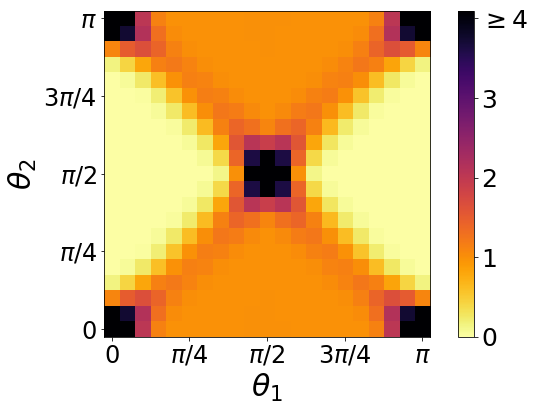
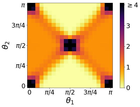
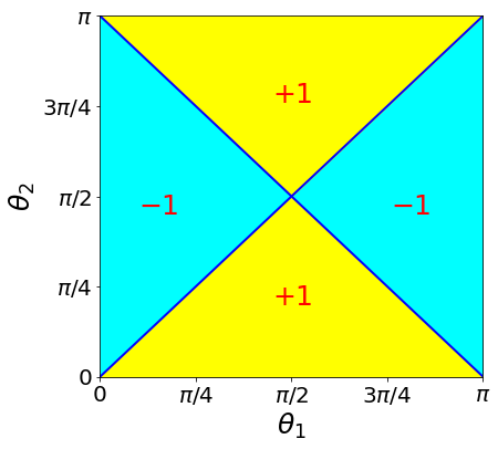
Figure 3: Half of the total quasienergy-averaged transmission $\overline{T}$, for two-dimensional quantum walks with position-independent parameters $\theta_{j},\alpha_{j},\beta_{j}$, and with maximally disordered $\phi$. Contribution to $\overline{T}$ from all even input channels is shown; odd input channels have contribution that is indistinguishable. Results are independent of the magnetic parameters (set to $\alpha_{1}=0.25\pi$, $\alpha_{2}=0.4\pi$, $\beta_{1}=0.1\pi$, $\beta_{2}=0.3\pi$). Dependence of the transmission on $\theta_{1}$ and $\theta_{2}$ is shown, with (a) a cut of type $A$, (b) a cut of type $B$, and (c) no cut. Without cuts, Anderson localized phases with low transmission are separated by lines of large transmission. With cuts, we have quantized transmission of 1 (total transmission of 2) in topological phases where edge states contribute to the transmission. (d) shows the values of the invariant for the translation invariant case, Eq. (17), which is in good agreement from the combination of (a)-(c) according to Eq. (28).

We illustrate how the method of obtaining topological invariants from total transmission with and without cuts works by numerical results, for the two-dimensional quantum walk with position-independent $\theta$, $\alpha$ and $\beta$ parameters, but completely disordered $\phi$.

We expect from previous work Edge and Asbóth (2015) that the topological invariant should be given by Eq. (17). We calculated transmission for $t_{\text{max}}=2000$ timesteps, on a system size of $L_{x}=39$ and $L_{y}=60$, considering only even input channels (odd channels have identical contribution). The results, shown in Fig. 3, largely confirm our expectations. We see anomalous Floquet-Anderson insulator phases characterized by low transmission in the case without cuts, and to a good approximation quantized transmission in the case with cuts (total transmission of 1 for even input channels is shown, same results for odd input channels were obtained), topological invariants matching up with Eqs. (28) and (17). These insulating phases are separated by lines of critical states, where transmission is high both with and without cuts. For the cases where quasienergy-averaged total transmission was 1, this was due to a single open channel (transmission eigenvalue $\approx$ 1), with other channels almost completely closed (transmission eigenvalue $\approx$ 0), as illustrated by a concrete example in Fig. 2. We defer analysis of the finite-size scaling of the total transmission near the topological phase transition to the next section.

IV Disorder in phase and magnetic parameters

Before turning to the two-dimensional quantum walk with all parameters random, we revisit the problem of a quantum walk with fixed $\theta$ parameters and fully random $\alpha,\beta$ or $\phi$. When disorder is only in the phase $\phi$, this reduces to the case of the split-step quantum walk, studied in Ref. Edge and Asbóth (2015), since position independent angle parameters $\alpha$ and $\beta$ can always be gauged away. There, it was found that in the simple split-step walk, with angle parameters $\theta_{1},\theta_{2}$ fixed to generic values, phase disorder leads to Anderson localization. On the other hand, when $\theta_{1},\theta_{2}$ is tuned to a topological phase transition, phase disorder leads to a diffusive spread of the wavefunction—a consequence of the critical nature of the system.

The numerical results in this section complement those of Ref. Edge and Asbóth (2015) by (1) a more in-depth analysis of the way the wavefunction of an initially localized particle spreads, (2) different numerical tools, the analysis of level repulsion statistics and of the finite-size scaling of transmission. We will also investigate the effect of having disorder not in $\phi$, but in the vector-potential-like parameters $\alpha$ and $\beta$. This is very similar to having onsite phase disorder but in a spin-dependent way Edge and Asbóth (2015). Before showing our numerical results, we discuss a technical detail that makes the simulation more efficient: a rotated basis.

IV.1 Rotated basis

Figure 4: The rotated basis for the quantum walk, with squared-shape unit cells containing two sites each from different sublattices (different symbols), and unit cell indices $n_{+}$ and $n_{-}$ shown. For a walk started from $x=0,y=0$, i.e., the $\square$ site in unit cell $n_{+}=n_{-}=0$, the walk only progresses along the solid and empty arrows (in the $s=1$ and $s=-1$ state, respectively).

For the time evolution of the quantum walk with fixed $\theta_{1,2}$, we used a rotated basis, with square-shaped unit cells containing two sites each from different sublattices, as shown in Fig. 4. Because of the sublattice symmetry, for a walk started from one sublattice, at any time during its time evolution, its wavefunction will only have support on at most one site per unit cell. Thus it is enough to keep track of the integer valued unit cell indices $n_{+}$ and $n_{-}$, and discard the sublattice information. On the $(e,e)$ and $(o,o)$ sublattices, these unit cell indices, and the corresponding coordinates $x_{\pm}$, are related to the integer valued site coordinates $x,y$ by

$$n_{\pm} =\frac{y\pm x}{2}; x_{\pm} =\frac{y\pm x}{\sqrt{2}}.$$ (30)

When rewriting the timestep operator of the quantum walk in this rotated basis, we need to start with the shifts defined in Eq. (5). For the quantum walk started from the $(e,e)$ or $(o,o)$ sublattice (a square in Fig. 4), we need

$$\hat{S}_{1\square} =\sum_{n_{+},n_{-}}\Big{(}|{n_{+},n_{-}-1,+1}\rangle\langle{n_{+},n_{-},+1}|$$

$$\quad\quad+|{n_{+}-1,n_{-},-1}\rangle\langle{n_{+},n_{-},-1}|\Big{)};$$ (31a)

$$\hat{S}_{2\square} =\sum_{n_{+},n_{-}}\Big{(}|{n_{+}+1,n_{-}+1,+1}\rangle\langle{n_{+},n_{-},+1}|$$

$$\quad\quad+|{n_{+},n_{-},-1}\rangle\langle{n_{+},n_{-},-1}|\Big{)},$$ (31b)

and obtain the timestep operator as

$$\hat{U}_{\square} =\hat{F}\hat{S}_{2\square}\hat{R}_{2}\hat{S}_{1\square}\hat{R}_{1},$$ (32)

where the parameters of the operators $\hat{F}$, $\hat{R}_{j}$ have to be chosen to match the position of the walker.

For the sake of completeness, a quantum walk started from the $(o,e)$ or $(e,o)$ sublattices (circle in Fig. 4) has modified shifts,

$$\hat{S}_{1\circ} =\sum_{n_{+},n_{-}}\Big{(}|{n_{+}+1,n_{-},+1}\rangle\langle{n_{+},n_{-},+1}|$$

$$\quad\quad+|{n_{+},n_{-}+1,-1}\rangle\langle{n_{+},n_{-},-1}|\Big{)};$$ (33a)

$$\hat{S}_{2\circ} =\sum_{n_{+},n_{-}}\Big{(}|{n_{+},n_{-},+1}\rangle\langle{n_{+},n_{-},+1}|$$

$$\quad\quad+|{n_{+}-1,n_{-}-1,-1}\rangle\langle{n_{+},n_{-},-1}|\Big{)},$$ (33b)

and timestep operator,

$$\hat{U}_{\circ} =\hat{F}\hat{S}_{2\circ}\hat{R}_{2}\hat{S}_{1\circ}\hat{R}_{1}.$$ (34)

With the rotated basis, a factor of two is gained in efficiency for the representation of the wavefunction, i.e., an array of size $L_{+}\times L_{-}$ is enough for a simulated area of $L_{+}\times L_{-}$ unit cells with $2L_{+}L_{-}$ sites. Besides, we will show later that during time evolution, the disorder-averaged position distribution is generically anisotropic, and elongated either along the diagonal or along the anti-diagonal direction (in the original, $x$-$y$ basis), depending on the values of $\theta_{1}$ and $\theta_{2}$. Thus, to minimize finite-size effects, it is more efficient to use rectangular rather than square shaped simulation area, elongated along the direction in which the position distribution is elongated, i.e., rotated by $45^{\circ}$. This is straightforward to implement in the rotated basis.

IV.2 Time evolution of wavefunction

A direct test of Anderson localization is simulation of the time evolution of the wavefunction for a particle started from a single site. In case of Anderson localization, the root-mean-squared displacement (distance from the origin, square root of the variance of position) remains bounded, and the long-time limiting form of the disorder-averaged probability distribution falls off exponentially with distance from the origin. In contrast, for a critical system, diffusive spread of the wavefunction is expected, with position variance increasing linearly with time, and the disorder-averaged probability distribution approaching a Gaussian shape. Both signatures for both cases have been observed for the split-step quantum walk with phase disorder Edge and Asbóth (2015), although for a limited range of parameters, with $\theta_{1}+\theta_{2}=\pi/2$. As we show below, departing from this limitation on the rotation angles $\theta$ changes the dynamics qualitatively, introducing anisotropy.

For the numerical simulation, we found it advantageous to work with absorbing boundary conditions. Absorbing boundary conditions, as already used for the scattering calculation in Sec. III.1, simply means setting the value of the wavefunction at the boundary to 0 at the end of every timestep. This allows us to track the finite-size error, or the “leaving probability” directly by the norm of the wavefunction,

$$p_{\text{leave}}=1-\sum\limits_{n_{+}=1}^{L_{+}}\sum\limits_{n_{-}=1}^{L_{-}}\sum\limits_{s=\pm 1}|\psi_{n_{+},n_{-},s}(t_{\text{max}})|^{2}.$$ (35)

Note that the absorbing boundary conditions as defined here are a “quick-and-dirty” way to emulate a finite segment of an infinite plane: in fact, a small part of the wavefunction is reflected back from the absorbing boundaries. Such reflections are numerical artifacts, which we can estimate by monitoring the error $p_{\text{leave}}$.

Figure 5: Disorder-averaged (envelope of the) position distribution, for two-dimensional quantum walks with position-independent $\theta_{j},\alpha_{j},\beta_{j}$, and maximally disordered $\phi$, together with fitted curves (shown in half of the semi-log plot). In (a), a generic case, with $\theta_{1}=0.2\pi$, and $\theta_{2}=0.4\pi$, we find Anderson localization, with good fit from Eq. (37) for the average over 100 disorder realizations after 10000 timesteps. In (b), with $\theta_{1}=\theta_{2}=0.2\pi$, we have a critical case with diffusive spread, with a good fit from Eq. (38) for the average over 10 disorder realizations after 3000 timesteps.

We have noticed that the disorder-averaged shape of the position distribution as the wavefunction of the quantum walk spreads is anisotropic, with contour lines having elliptical shapes, ellipses elongated either along the diagonal ($x+y$) or along the antidiagonal ($x-y$) direction. Typical examples are shown in Fig. 5. The direction of elongation depends on the parameters $\theta_{j}$, following a harlequin pattern, which can be put in a concise (although somewhat obfuscated) formula: the dominant direction is

$$x\pm y,\quad\text{with }\,\,\pm =\text{sgn}\left[\cos(\theta_{1}-\theta_{2})\cos(\theta_{1}+\theta_{2})\right],$$ (36)

with an isotropic position distribution if $\cos(\theta_{1}-\theta_{2})\cos(\theta_{1}+\theta_{2})=0$. We do not have a complete understanding of why the elliptical contour lines are not rotated by any angle other than $\pm 45^{\circ}$. There are, however, two special cases that are straightforward to check by considering two consecutive timesteps (as in Ref. Asbóth (2012) for a one-dimensional quantum walk). If either $\theta_{1}$ or $\theta_{2}$ is set to $n\pi$, the quantum walk is one-dimensional, spreading only along the diagonal. If either $\theta_{1}$ or $\theta_{2}$ is set to $(n+1/2)\pi$, it spreads only along the anti-diagonal (hence if one of them is $n\pi$, the other $m\pi+\pi/2$, with $n,m\in\mathbb{Z}$, no spreading at all). This is consistent with Eq. (36).

We now turn to the rate at which the position distribution spreads and its shape in the long-time limit, to find signatures of Anderson localization vs. diffusion. For generic cases, i.e., when $\theta_{1}\neq\pm\theta_{2}+n\pi$, with $n\in\mathbb{N}$, with maximal phase disorder, we find signatures of Anderson localization. The envelope of the disorder-averaged position distribution in the long-time limit can be fitted very well with

$$p(x_{+},x_{-},t) \propto\exp\left[-\sqrt{\left(\frac{x_{+}}{\zeta_{+}(t)}\right)^{2}+\left(\frac{x_{-}}{\zeta_{-}(t)}\right)^{2}}\,\right],$$ (37)

where $\zeta_{+}$ and $\zeta_{-}$ increase slowly with time (we expect them to saturate in the long-time limit); these denote the localization lengths along the diagonal and anti-diagonal directions, with the variance of the position given by $\langle{x^{2}+y^{2}}\rangle\approx 3(\zeta_{+}^{2}+\zeta_{-}^{2})$. By “envelope”, we mean that on every second site the wavefunction is 0 because of sublattice symmetry. Eq. (37) is an exponentially localized form, with contours that have elliptic shapes, tilted by $45^{\circ}$. We show an example in Fig. 5(a), where $\theta_{1}=0.2\pi$, $\theta_{2}=0.4\pi$, and the fitted values of the localization lengths are $\zeta_{+}=3.7$ and $\zeta_{-}=6.7$ (with maximal disorder in the magnetic parameters as well, $\zeta_{+}=3.5$ and $\zeta_{-}=6.8$).

For the critical cases, i.e., when $\theta_{1}=\pm\theta_{2}+n\pi$, the wavefunction spreads out in a diffusive way. We find that a good fit for the envelope is

$$p(x_{+},x_{-},t)\propto\exp\left[-\frac{x_{+}^{2}}{4D_{+}t}-\frac{x_{-}^{2}}{4D_{-}t}\right],$$ (38)

with $D_{+}$ and $D_{-}$ denoting the diffusion coefficients along the diagonal and antidiagonal directions, with the variance of the position given by $\langle{x^{2}+y^{2}}\rangle\approx 2(D_{+}+D_{-})t$. We show an example in Fig. 5(b), where $\theta_{1}=\theta_{2}=0.2\pi$, and the fitted values of the diffusion coefficients are $D_{+}=1.1$ and $D_{-}=0.31$ (unaffected by maximal disorder in the magnetic parameters).

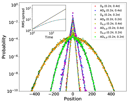
Figure 6: Diagonal (D, along $x_{-}=0$, only even $x_{+}$) and antidiagonal (AD, along $x_{+}=0$, only even $x_{-}$) cuts of the position distributions of Fig. 5 (semi-log plot). Phase disorder (suffix $\phi$) and disorder in magnetic parameter (suffix $\alpha,\beta$) give almost indistinguishable results. Continuous lines show the fitted theory curves—they are almost completely covered by the numerical data points, indicating excellent fit, except for the close vicinity of the origin. The inset shows the time dependence of the square root of the variance (log-log plot), which scales diffusively for the critical case and appears to approach saturation for the generic case.

We show more details on diagonal and antidiagonal cuts of the disorder-averaged position distributions in Fig. 6. We took these cuts from the simulation runs represented in Fig. 5. We note that the parameters $\zeta_{\pm}$ and $D_{\pm}$ in Eqs. (37) and (38) were obtained by fitting the analytical curves to these cuts. The fits, as already seen in Fig. 5, are quite good, except for the diffusive case in the vicinity of the origin, where we observe a spike (more on this in Sec. VI.3). We also plot in Fig. 6 the numerical results for cases with the maximal disorder taken in $\alpha$ and $\beta$, rather than in $\phi$; the effects of these two types of disorder are the same, consistent with previous results Edge and Asbóth (2015). In the inset we show the measured time dependence of the root-mean-squared width. For the critical case, $\theta_{1}=\theta_{2}=0.2\pi$, this is a linear function on the log-log plot, with $\sqrt{\langle{x^{2}+y^{2}}\rangle}=1.5t^{0.5}$, i.e., diffusive scaling. For the generic case, $\theta_{1}=0.2\pi$, $\theta_{2}=0.4\pi$, the variance grows slower, consistent with the expectation that it would eventually saturate.

IV.3 Level spacing statistics

A frequently used tool to characterize Anderson localization/criticality is the level spacing statistics Sepehrinia and Sheikhan (2011). As often applied in Hamiltonian systems, first an energy $E$ is fixed, and then from each disorder realization the gap around $E$ is taken, i.e., $\delta_{j}=\varepsilon_{+,j}-\varepsilon_{-,j}$, with $\varepsilon_{\pm,j}$ denoting the first level above/below $E$ in the $j$th disorder realization. The ensemble of normalized level spacings $s_{j}$ is then defined as

$$s_{j} =\frac{\delta_{j}}{\langle{\delta}\rangle},$$ (39)

with $\langle{\ldots}\rangle$ denoting the disorder average.

In an Anderson localized system, eigenstates separated by large distances cannot be coupled by local perturbations, therefore their energies (in our case, quasienergies) are essentially independent. Thus the normalized level spacing has exponential probability distribution (in this context also called Poissonian),

$$p(s) =p_{\text{loc}}(s)=e^{-s},$$ (40)

with $p(s)$ denoting the probability density. In a critical system, on the other hand, the eigenstates have extended wavefunctions, which can be coupled by local perturbations and hybridize, and therefore we expect level repulsion to occur. The normalized level spacings in this case are expected to follow a Wigner–Dyson distribution, which for the case relevant for us (so-called Gaussian Unitary Ensemble) reads,

$$p(s) =p_{\text{GUE}}(s)=\frac{32}{\pi^{2}}s^{2}e^{{-{\frac{4}{\pi}}s^{2}}}.$$ (41)

When we compute level spacing statistics for quantum walks, we need to pay attention to the sublattice structure (see Sec. II.1). The timestep operator $\hat{U}$ of a walk describes two independent quantum walks, taking place on different sublattices ($x+y=$ even vs. $x+y=$ odd). Thus $\hat{U}$ has two sets of energy levels whose level spacing distributions should be calculated separately (just as in the case of Hamiltonians with unitary symmetries): There can be no level repulsion between levels from different sets. To account for this, we start from the spectrum of $\hat{U}^{2}$, to obtain that of $\hat{U}$, as in Sec. II.1. For a quantum walk on $2N$ sites (with $N$ even, and with proper boundary conditions), we need to diagonalize the $N\times N$ blocks of $\hat{U}^{2}$ on the $(e,e)$ sublattice (denoted by $\square$ in Fig.  4), and on the $(e,o)$ sublattice (denoted by $\circ$). From the corresponding eigenvalues of $\hat{U}^{2}$, namely, $e^{2i\varepsilon^{\square}_{j}}$ and $e^{2i\varepsilon^{\circ}_{j}}$, with $1\leq j<N$, and $0\leq\varepsilon^{\square/\circ}_{j}<\pi$, we obtain the $2N$ independent quasienergy level spacings of the spectrum of $\hat{U}$ as

$$\delta^{\square}_{j} =(\varepsilon^{\square}_{(j+1)\text{ mod }N}-\varepsilon^{\square}_{j})\mod\pi,$$ (42)

with $j=1,\ldots,N$, and with analogous definitions for $\delta_{j}^{\circ}$.

Having maximal phase disorder, i.e., $\phi$ of Eq. (2) equidistributed in the interval $[-\pi,\pi)$, gives us a huge boost in numerical efficiency for obtaining the level statistics. As already discussed in Sec. III.3, we can treat all of the quasienergies on the same footing and for a quantum walk on $2L_{+}L_{-}=2N$ sites ($N$ cells in the rotated basis) obtain $2N$ values of normalized level spacing as

$$s_{j} =\frac{N}{\pi}\delta_{j}^{\square}; s_{j+N} =\frac{N}{\pi}\delta_{j}^{\circ},$$ (43)

with the level spacings $\delta^{\square}_{j}$ and $\delta^{\circ}_{j}$ for $j=1,\ldots,N$ defined in Eq. (42). Thus, we obtain a level spacing ensemble of size $2N$ by only diagonalizing two unitary matrices—a boost in numerical efficiency. On the downside, to obtain all the level spacings we fully diagonalize these large unitaries of size $N\times N$, where $N=L_{+}L_{-}$, with a numerical cost of $O(N^{3})$. This constrains us to system sizes of the order of $N\approx 20000$, which turns out to be large enough for the cases we considered here. We could go beyond that by repeatedly sampling the spectrum of $\hat{U}^{2}$ using iterative algorithms that obtain only part of the spectrum, such as the Arnoldi method Lehoucq et al. (1998) (which works applies ideas used in the Lanczos algorithm to more general matrices).

Figure 7: Level-spacing distributions for the quantum walks of Fig. 6. Angle parameters $(\theta_{1},\theta_{2})$ were fixed, at ($0.2\pi,0.4\pi$)—localized—or ($0.2\pi,0.2\pi$)—diffusive. For both cases, we considered maximal phase disorder (blue dots, green squares, respectively) or magnetic phase disorder (yellow triangles, purple crosses, respectively). For each parameter set a single disorder realization was used. Calculations were done in the rotated basis with periodic boundary conditions, with system size optimized for numerical efficiency: $L_{+}=112,L_{-}=196$ for the localized cases, $L_{+}=204,L_{-}=110$ for the diffusive cases. Lines show the theoretical distributions, which fit well with the numerical data [dashed: Eq. (40) and continuous: (41), with no free parameters]. For better visibility we terminate the horizontal axis at $s=4$; in the case with $\theta_{1}=0.2\pi$ and $\theta_{2}=0.4\pi$, we observed even larger normalized level spacings, almost up to $s=10$. Semilogarithmic inset shows that in the diffusive case, for large $s$ the distribution is systematically above the Wigner-Dyson formula, and falls off roughly exponentially. For the inset, to have enough statistics in the critical case, we diagonalized 100 disorder realizations of a system with $L_{+}=136$, $L_{-}=74$.

We show numerically obtained level spacing distributions, and the theoretical expectations for them, in Fig. 7. Here we used the same examples as in Fig. 6: a generic quantum walk with $\theta_{1}=0.2\pi$, $\theta_{2}=0.4\pi$ and a critical quantum walk with $\theta_{1}=\theta_{2}=0.2\pi$—in both cases, results collected from a single sublattice are shown. For both cases we considered two types of maximal disorder: disorder in $\phi$ and $\alpha,\beta$ fixed or the other way around. For the critical case, we see reasonable agreement between the level spacing distributions and the Wigner-Dyson distribution of Eq. (41), with slight deviations. Notably, we see more instances of large level spacings than Wigner-Dyson would predict, their number appears to fall off roughly exponentially for $s>2.5$ rather than according to a Gaussian tail, as shown in a logarithmic inset. Such a departure of the level spacing statistics from Wigner-Dyson has also been seen at critical points of the two-dimensional Anderson transition Obuse and Yakubo (2005). For the generic, Anderson localized case, we observe a very good agreement with the exponential distribution of Eq. (40), with some level repulsion showing up at the $s\ll 1$ end—states that are almost degenerate—which we attribute to finite size effects. Using the rotated basis for these calculations, allowed us to adapt the shape of the simulated area to the expected shape of the wavefunctions, and thus minimize finite-size effects.

IV.4 Scaling of transmission

The calculation of the transmission matrix of a disordered two-dimensional quantum walk gives us yet another numerical tool to differentiate between Anderson localization and diffusive spread. Scaling up the system size while keeping the system shape constant, total transmission across an insulator should decrease exponentially, while for the diffusive case (e.g., a metal), we expect a total transmission that is roughly constant Nazarov et al. (2009).

For the finite-size scaling of the transmission, we calculated quasienergy- and disorder-averaged total transmissions for three different system sizes with the same shape of $L_{y}/L_{x}=3/2$ (together with the extra column of sites for the leads), for different values of $\theta_{1}$ and $\theta_{2}$. We kept $\theta_{1}+\theta_{2}=0.6\pi$, and used values of $\theta_{1}$ from $\pi/10$ to $\pi/2$, thus tuning the system across a topological phase transition which takes place at $\theta_{1}=\theta_{2}=0.3\pi$. For each value of $\theta_{1},\theta_{2}$, we calculated transmission for three different system sizes, $L_{x}=19,L_{y}=30$; $L_{x}=39,L_{y}=60$; and $L_{x}=59,L_{y}=90$. We used Eq. (29), for the numerics, with the number of timesteps $t_{\text{max}}$ chosen such that the incident walker from any input lead will have left the system with probability above $99\%$, namely, $t_{\text{max}}=1000$ for $L_{x}=19,L_{y}=30$; $t_{\text{max}}=2000$ for $L_{x}=39,L_{y}=60$; and $t_{\text{max}}=3000$ for $L_{x}=59,L_{y}=90$. This criterion for choosing $t_{\text{max}}$ can be written using Eq. (35) as $p_{\text{leave}}>0.99$, with the conditional wavefunction $|{\Psi_{n}(t+1)}\rangle=\hat{U}(\hat{\Pi}_{\text{sys}}\hat{U})^{t}|{0,n,+1}\rangle$.

Figure 8: Finite-size scaling of the quasienergy-averaged total transmission for quantum walks with maximal phase disorder but fixed $\theta_{1}$ and $\theta_{2}$. Results for three different system sizes are shown, with fixed aspect ratio $L_{y}/L_{x}=3/2$. Ten disorder realizations were used for each setting, with individual results shown by markers and averages by lines. The inset shows the transmission data on a semilogarithmic scale, confirming exponential decrease of total transmission for the cases with $\theta_{1}\neq\theta_{2}$ as the system size is scaled up.

Our numerical results for the quasienergy-averaged total transmission, shown in Fig. 8, confirm that tuning $\theta_{1}$ and $\theta_{2}$ indeed drives the quantum walk with complete phase disorder across a quantum phase transition between different localized phases. We observe that for $\theta_{1}\neq\theta_{2}$, the total transmission decreases exponentially (see semilogarithmic plot in the inset). For $\theta_{1}=\theta_{2}=0.3\pi$, on the other hand, the transmission is unchanged as the system size is scaled up, a numerical signature of diffusive transport.

V Haar random quantum walk is diffusive

We finally turn to the question raised in the title: Is the completely disordered two-dimensional quantum walk Anderson localized or does it spread out to infinity? Thus, we take a two-dimensional quantum walk as in Eq. (7), with both rotation operators $\hat{R}_{j}$ chosen randomly from $U(2)$ according to the Haar measure Mezzadri (2006), i.e., Haar random operators.

We can realize Haar random coins with the operators of Eqs. (2) and (4) by taking their parameters from properly defined distributions Ozols (2009). The parameters $\alpha_{j}(x,y)$, $\beta_{j}(x,y)$, with $j=1,2$, and $\phi(x,y)$ have to be uncorrelated random variables, uniform in the interval $[-\pi,\pi)$. The parameters $\theta_{j}(x,y)$ need to be generated as

$$\theta_{j}(x,y) =\arcsin\Big{(}\sqrt{\zeta_{j}(x,y)}\Big{)}$$ (44)

with $\zeta_{j}(x,y)$ uncorrelated uniform random in the interval $[0,1]$.

Figure 9: Position distribution of the Haar random two-dimensional quantum walk after 10000 timesteps, with fitted theoretical distribution, Eq. (38) (semi-log plot). No disorder averaging used, result from a single disorder realization is shown. Absorbing boundary conditions were used, the leaving probability from the boundary is $p_{\text{leave}}<10^{-9}$.

In Fig. 9 the position distribution is shown after 10000 timesteps on a system of size $1001\times 1001$. Even without disorder averaging, the distribution is quite smooth and roughly isotropic. It corresponds to a Gaussian, can be fitted quite well with the diffusive ansatz of Eq. (38), with diffusion coefficients $D_{+}=D_{-}=0.54$. In Fig. 10, we show the fit with the diffusive curve of the cross-sectional cut of the disorder-averaged position distribution (from 200 random realizations, after 1500 timesteps) of the Haar random quantum walk. It is only near the origin that the Gaussian fit is not very good; as shown in the inset, we find here a pronounced peak, just as with the phase disordered quantum walks of Fig. 6. We analyze this peak in more detail later in Sec. VI.3. The simulations of Fig. 10 were run on systems of $501\times 501$ unit cells in the rotated basis, with absorbing boundary condition, error $p_{\text{leave}}<10^{-15}$.

Figure 10: Cross-sectional cut of the position distribution of Fig. 9, with the fitted Gaussian curve (semi-log plot). Results for the $D$ and $AD$ cross-sectional cuts were indistinguishable; we show their average here. The fit is excellent, everywhere, except for the small local peak near the origin—shown in an inset. A second inset shows the time dependence of the root-mean-square-width of the full position distribution (log-log plot), which matches well with a diffusive scaling $\sqrt{\langle{r^{2}(t)}\rangle}=1.4\cdot\sqrt{t}$.

We also have numerical evidence—shown in Fig. 10—that coherence plays almost no role in the way the Haar random quantum walk spreads. We show on the plot the position distributions of two classicalized variants of the quantum walk, after the same number of timesteps, on a same system size. The first classicalized variant is a time-dependent Haar random quantum walk, obtained by generating new disorder realizations of the rotation matrices for every timestep (average of 200 random realizations of the walk is shown). The second classicalized variant was obtained with a single disorder realization but with all coherence omitted from the quantum walk. Here, we replaced the unitary timestep operator $\hat{U}$ of Eq. (7)–more precisely, of Eq. (32)—with the corresponding stochastic operator, i.e., replaced all complex phase factors by 1 and the parameters $\pm\sin\theta_{j}(x,y)$ and $\cos\theta_{j}(x,y)$ by $\sin^{2}\theta_{j}(x,y)$ and $\cos^{2}\theta_{j}(x,y)$, respectively. For this second classicalized variant, the positive-valued function $\Psi(x,y)$ is interpreted as probability instead of probability amplitude. Here no disorder averaging was needed, as a single random realization already gave results with negligible statistical fluctuations.

Figure 11: Level spacing distribution for the Haar random two-dimensional quantum walk on a $160\times 160$ square lattice, on the rotated basis, with periodic boundary conditions. The distribution shows signs of criticality; it is very close to the Wigner-Dyson distribution, Eq. (41), and not to the exponential distribution of Eq. (40) typical for Anderson localization. Semilogarithmic inset shows that for large $s$ the distribution is systematically above the Wigner-Dyson formula and falls off roughly exponentially—in the same way as for the diffusive case in Fig. 7. For the inset, to have enough statistics, we diagonalized 100 disorder realizations on a system with $L_{+}=L_{-}=100$.

Figure 12: Finite-size scaling of the quasienergy-averaged total transmission for Haar random two-dimensional quantum walk. As system size is increased by a factor of 4, keeping aspect ratio at $L_{y}/L_{x}=3/2$, total transmission is roughly a constant, indicating diffusive transmission. Forty disorder realizations were used for each setting; individual results are shown by markers and averages by lines.

Figure 11 shows the level spacing distribution, which matches quite well the Wigner-Dyson distribution of Eq. (41). As in the case of the critical quantum walk with fixed $\theta_{1}=\theta_{2}$ (Fig. 7), we again see small deviations, notably the probability of large values of the level spacing $s$ seems to fall off exponentially with $s$, as shown in the logarithmic inset (as in the two-dimensional Anderson transition Obuse and Yakubo (2005)). Good agreement with Wigner-Dyson indicates the presence of extended states—or, in other words, the absence of Anderson localization. The distribution was obtained for a single disorder realization, on a $160\times 160$ lattice, on the rotated basis, with periodic boundary conditions.

The quasienergy-averaged total transmission, shown in Fig. 12, is roughly unchanged as the system size is increased by a factor of 4, again indicating diffusive transmission. We used Eq. (29) for the transmission calculations, with parameters similar to those of Fig. 8, i.e., four different system sizes, with integration times $t_{\text{max}}$ matched for error $<0.01$, namely, $L_{x}=19,L_{y}=30,t_{\text{max}}=1000$; $L_{x}=39,L_{y}=60,t_{\text{max}}=2000$; $L_{x}=59,L_{y}=90,t_{\text{max}}=3000$; $L_{x}=79,L_{y}=120,t_{\text{max}}=4000$.

Figure 13: Probability distribution of the quantum walk parameters $(\theta_{1},\theta_{2})$, when they are selected according to Eq. (44) to realize the Haar uniform distribution, with the corresponding value of the topological invariant ($\pm 1$) shown. Because of the symmetry of the distribution, pairs of points $(\theta_{1},\theta_{2})$ and $(\theta_{2},\theta_{1})$ have the same probability density. These pairs have opposite topological invariant—see also Fig. 3—but lead to the same localization lengths in the maximally disordered phase limit.

The diffusive spread of the Haar random two-dimensional quantum walk is due to disorder-induced topological criticality. Parameters $\alpha$ and $\beta$ have no impact on the topological phase, which is determined solely by $\theta_{1}$ and $\theta_{2}$. Although we are not sampling $\theta_{1}$ and $\theta_{2}$ uniformly, as in Ref. Edge and Asbóth (2015), we are using a distribution, using Eq. (44), shown in Fig. 13, which has the same probability density for $(\theta_{1},\theta_{2})=(\theta_{A},\theta_{B})$ as $(\theta_{1},\theta_{2})=(\theta_{B},\theta_{A})$, for any $\theta_{A},\theta_{B}$. Thus, the qualitative argument used from Ref. Edge and Asbóth (2015), related to network models of topological phase transitions, still applies.

VI Haar random quantum walk is critical

In the previous section, we have shown that the Haar random quantum walk spreads diffusively, which we attributed to a topological delocalization. Briefly summarized, we picked the coin operators in an unbiased random way, uniformly according to the Haar distribution. Had we deviated from this unbiased randomness by distorting the distribution in a generic way, we would have obtained a highly disordered two-dimensional quantum walk, with a bulk topological invariant (winding number) that is +1 or -1, depending on the deviation. Thus the Haar random quantum walk is a critical case between quantum walks that have localized bulk and topologically protected edge states—just like the critical quantum walk of Sec. IV.

We expect based on the arguments above that the Haar random quantum walk should not only evade Anderson localization, but also display the same type of critical behavior as the integer quantum Hall effect. In the integer quantum Hall effect too, tuning to a transition between two phases with different Chern numbers results in a divergence of the bulk localization length, which is required because edge states on opposing edges need to hybridize in order for the Chern number to change. This rough analogy between these two topological transitions has been precisely phrased for anomalous Floquet-Anderson insulators using field theoretic tools Kim et al. (2020).

We substantiate the topological delocalization picture by extracting a critical exponent used in the integer quantum Hall effect from the numerical results on the Haar random and the critical quantum walks. This is the exponent $\eta$, which characterizes critical wavefunction Huckestein (1995) by (1) describing the autocorrelation of the position distribution, (2) controlling the fractal scaling of the second moment of the position distribution, and (3) controlling the time decay of the probability of return to the origin. We use each of these three properties to extract numerical values for $\eta$. We have found that these approaches roughly agree and give $\eta\approx 0.52$, which is consistent with the value of $\eta$ for the integer quantum Hall effect ($\eta=0.524\pm 0.003$ in Ref. Evers et al. (2008)).

VI.1 Autocorrelation of position distribution

The first method to obtain the critical exponent $\eta$ is via the autocorrelation function of the position distribution of the eigenstates. For a random realization of the disorder, we obtain eigenstates of $\hat{U}^{2}$ using sparse matrix diagonalization (in the rotated basis, with periodic boundary conditions, obtained using the Arnoldi method with shift-invert, with quasienergies $\varepsilon\approx 0$). Because of the sublattice symmetry, as discussed in Sec. II.1, each eigenvalue $e^{-i\varepsilon}$ of $\hat{U}^{2}$ is twice degenerate, with eigenstates $|{\Psi_{1}}\rangle$ and $|{\Psi_{2}}\rangle$. We can obtain the position distribution corresponding to eigenstates of $\hat{U}$ with eigenvalue $\pm e^{-i\varepsilon/2}$ by summing over the two degenerate eigenstates,

$$p(n_{+},n_{-}) =\frac{1}{2}\sum_{j=1,2}\sum_{s=\pm 1}{\left|{\Psi_{j}(n_{+},n_{-},s)}\right|}^{2}.$$ (45)

The autocorrelation function $R(r)$ is obtained from the position distribution for various values of $r$, as

$$R(r) =\sum_{n_{+}=1}^{L_{+}}\sum_{n_{-}=1}^{L_{-}}p(n_{+},n_{-})p(n_{+}+r~{}\text{mod}~{}L_{+},n_{-}).$$ (46)

For critical wavefunctions, this autocorrelation function decays as a power law as a function of distance Huckestein (1995), with exponent $-\eta$, i.e.,

$$\overline{R(r)}\propto r^{-\eta}.$$ (47)

Here, the overbar denotes averaging over all eigenstates (different disorder realizations and various quasienergy values).

Figure 14: Autocorrelation of position distributions of eigenstates of (a) Haar random quantum walk and (b) a critical quantum walk with $\theta_{1}=\theta_{2}=0.2\pi$ with maximal phase disorder (disorder in magnetic parameter gave indistinguishable results). For both cases, 400 position distributions of eigenstates were calculated in the rotated basis, with periodic boundary conditions, on a lattice 512$\times$512 and 512$\times$256, respectively. Histograms of the logarithms of autocorrelation values for fixed $r$ (red shading) are consistent with power law decay; the fitted exponents are $\eta=0.516\pm 0.02$ and $\eta=0.510\pm 0.02$ in the two cases.

We show our numerical results on the autocorrelation $R(r)$ for both the Haar random quantum walk and for a critical quantum walk with fixed rotation angles $\theta_{1}=\theta_{2}=0.2\pi$ and maximal phase disorder, in Fig. 14. We calculated $R(r)$ for 8 values of $r$ from 400 position distributions (40 random disorder realizations, for each realization 20 eigenstates giving 10 position distributions because of twofold degeneracy). We show histograms of the logarithms of the autocorrelation values for all values of $r$. The distributions clearly vary around a linear function on the log-log plot, which confirms power law decay. We estimated $\eta$ by fitting a straight line to $\ln R$-$\ln r$. We omitted the values $r>L_{+}/4$, since the distributions at $r=L_{+}/2$ appear to be slightly above the expected value, influenced by the boundary conditions (which we confirmed by calculations at smaller system sizes). We also omitted the two smallest values of $r$ from the fit, to decrease the influence of lattice effects. We obtained $\eta=0.516\pm 0.02$ and $\eta=0.510\pm 0.02$ for the Haar random quantum walk and the critical quantum walk with fixed rotation angles, respectively (with 99.7% confidence level). These are compatible with $\eta=0.524\pm 0.03$ calculated for the critical states of the integer quantum Hall effect Evers et al. (2008).

VI.2 Fractal analysis of position distribution

The second method to obtain the critical exponent $\eta$ uses a fractal analysis of the position distribution of eigenstates at the transition. For each position distribution (obtained as detailed above), we coarse grained using boxes (squares) of side $l$ (we chose $l=2^{j}$ for integer $j$ values) and calculated averages of the squares of the coarse grained distributions,

$$\langle{p^{2}(l)}\rangle=\frac{l^{2}}{L_{+}L_{-}}\sum_{m_{+}=0}^{L_{+}/l-1}\,\sum_{m_{-}=0}^{L_{-}/l-1}[p_{l}(m_{+},m_{-})]^{2};\\ p_{l}(m_{+},m_{-})=\sum_{n_{+}=m_{+}l+1}^{m_{+}l+l}\,\sum_{n_{-}=m_{-}l+1}^{m_{-}l+l}p(n_{+},n_{-}).$$ (48)

For critical wavefunctions, this quantity increases with box size $l$ as a power law Huckestein (1995),

$$\overline{\langle{p^{2}(l)}\rangle}\propto l^{4-\eta}.$$ (49)

Figure 15: Fractal analysis of the position distributions of (a) the Haar random quantum walk and (b) a critical quantum walk with fixed rotation angles $\theta_{1}$ = $\theta_{2}$ = $0.2\pi$ with maximal phase disorder, using the same wavefunctions as for Fig. 14. Averages are calculated after various degrees of coarse graining as per Eq. (48). Histograms of the logarithms for fixed box size $l$ (red shading) are consistent with power law as per Eq. (49); the fitted exponents give $\eta=0.55\pm 0.02$ for the Haar random and $0.520\pm 0.015$ for the critical quantum walk with fixed rotation angles.

We show our numerical results on the fractality of $\langle{p^{2}}\rangle$ for both the Haar random and for a critical quantum walk with fixed rotation angles $\theta_{1}=\theta_{2}=0.2\pi$ and maximal phase disorder in Fig. 15. We used the same 400 position distributions as for the autocorrelation calculation above. We show the distributions of $\log(\langle{p^{2}(l)}\rangle)$, which are clustered around a straight line on a log-log plot, confirming the fractal scaling. The estimate of $\eta$ obtained by linear least-squares fit is $\eta=0.55\pm 0.02$, and $\eta=0.52\pm 0.01$ for the Haar random and the critical quantum walk with fixed rotation angles, respectively, both reasonably compatible with the value of $\eta$ in the integer quantum Hall effect.

VI.3 Time dependence of the position distribution peak at the origin

The third method to obtain the critical exponent is observing the time dependence of the probability of return to the origin. We have seen in the previous section that on large length scale, the Haar random quantum walk seems to spread diffusively, with the position distribution well approximated by a two-dimensional Gaussian [Eq. (38)] whose width increases linearly with time, and value near the origin decreases $\propto 1/t$. However, close to the origin, there is a peak that can be observed. The height of this peak is $p_{0}(t)$, the probability of being at the origin,

$$p_{0}(t)=\sum_{s=\pm 1}\left|{\Psi(0,0,s,t)}\right|^{2}.$$ (50)

For a diffusively spreading probability distribution, we would expect $p_{0}(t)\propto 1/t$. For time evolution of critical wavepackets, a power law with a different exponent is expected Huckestein (1995),

$$\overline{\langle{p_{0}(t)}\rangle}\propto t^{-1+\eta/2}.$$ (51)

Here we used the overbar to denote averaging over disorder realizations, with time-evolved wavefunctions all started in the state $|{0,0,+1}\rangle$.

We show our numerical results on the time dependence of the probability of return to the origin (more precisely, of being at the origin) for both the Haar random and for a critical quantum walk with fixed rotation angles $\theta_{1}=\theta_{2}=0.2\pi$ and maximal phase disorder in Fig. 16. For both cases we used 600 disorder realizations. Distributions of $\log(p_{0}(t))$ are clustered around a straight line on a log-log plot, confirming the power law decay. The estimate of $\eta$ obtained by linear least-squares fit is $\eta=0.48\pm 0.06$ for the Haar random quantum walk and $\eta=0.50\pm 0.06$ for the critical quantum walk with fixed rotation angles. Both values are compatible with $\eta=0.524\pm 0.03$ of the integer quantum Hall effect.

Figure 16: Time dependence of probability of being at the origin for (a) the Haar random quantum walk and (b) a critical quantum walk with fixed rotation angles $\theta_{1}=\theta_{2}=0.2\pi$ with maximal phase disorder. Histograms of $\log(p_{0}(t))$ are consistent with power law as per Eq. (51). Fitted linear to the averages on the log-log plot of (a) Haar random quantum walk has slope $-0.76\pm 0.03$, which gives $\eta=0.48\pm 0.06$, (b) critical quantum walk with fixed rotation angles has slope $-0.75\pm 0.03$, which gives $\eta=0.50\pm 0.06$.

VII Discussion and conclusion

We have studied Anderson localization and topological delocalization in two-dimensional split-step quantum walks with two internal (coin) states and complete phase disorder. We first reviewed the known case of phase disorder on walks with real coin operators, which results in an anomalous Floquet-Anderson insulator. Here we used the numerical tools of wavefunction spread, level spacing distribution, and scaling of transmission. We simulated wavefunction spread in a rotated basis, better adapted to the observed nonisotropic shape of the position distributions (elongated along the diagonal or antidiagonal direction in the $x$-$y$ basis). Moreover, we calculated the topological invariants for these disordered quantum walks using scattering theory, thus substantiating the topological explanation of the delocalization given in Ref. Edge and Asbóth (2015). We then have shown how the numerical tools and analytical arguments carry over to the case of completely disordered two-dimensional quantum walks, i.e., with $U(2)$ coin operators taken randomly and uniformly according to the Haar measure. We have found that this maximal disorder does not lead to Anderson localization but results in a diffusive spread of the quantum walk. The absence of localization is explained by the observation that Haar random disorder tunes the system to a critical state, between different anomalous Floquet-Anderson phases. We substantiated this explanation by calculating the critical exponent $\eta$ using three different approaches and found good agreement with the value for the quantum Hall effect.

Complete phase disorder was crucial in boosting the efficiency of the numerical tools we used by ensuring that—statistically speaking—all quasienergies are equivalent. This is quite different from the case of topological delocalization in one-dimensional chiral symmetric quantum walks Obuse and Kawakami (2011); Zhao and Gong (2015); Rakovszky and Asbóth (2015), which only happens at specific quasienergy values ($\varepsilon=0,\pi,\pm\pi/2$). We could thus interpret the time evolution of the spreading of the wavefunction in a straightforward way and use quasienergy averaging as a way of disorder averaging. We have found that this holds if complete disorder is in the phase $\phi$ or in the magnetic parameters $\alpha$ and $\beta$—as could be expected from earlier work Edge and Asbóth (2015).

It would be interesting to consider whether the topological delocalization occurs in split-step quantum walks in higher dimensions. For the one-dimensional case, Haar random coins result in Anderson localization, which has even been rigorously proven Ahlbrecht et al. (2011). There in the absence of any symmetries (Cartan class A), no topological invariant exists, and thus generic disorder destroys topological phases rather than drive the system to criticality. The same holds in every odd dimension Hasan and Kane (2010), and thus we expect Anderson localization for Haar random split-step quantum walks in any odd dimensions. However, in even dimensions we have the possibility of disorder-induced topological delocalization, and it would be interesting to find if this occurs, e.g., for four-dimensional split-step quantum walks with two internal states.

We also wonder how sensitive our conclusions are to the number of internal states of the quantum walk, which we set to two. Two internal states is the smallest number with which a discrete-time quantum walk can be constructed, but it requires the split-step construction for a quantum walks in two or more dimensions. Moving to higher number of internal states represents a challenge for the description of topological phases because of the higher number of coin parameters. Moreover, with a larger internal coin space, it is quite possible that the localization length would be significantly larger, making it harder to observe numerical signatures of Anderson localization.

Our work also points to some open problems concerning a more complete picture of the localization-delocalization transition in disordered two-dimensional quantum walks. First, we lack the precise condition for Anderson localization of quantum walks for more general types of disorder—we have such a precise condition for the one-dimensional case Rakovszky and Asbóth (2015)). We have made some first steps in this direction for the numerical investigation of binary disorder; the results are in Appendix. Second, we do not have an analytical understanding of why we obtain diffusion, rather than sub- or superdiffusion in the critical case. For both of these questions, mapping to network models of topological transitions Delplace et al. (2017), or other theoretical tools Kim et al. (2020), could be used.

Appendix: Localization under binary disorder in rotation angles

Figure 17: Total transmission $\overline{T}$ on one sublattice in a quantum walk with binary disorder—as described in Eqs. (52), (53), (54): (a) with a cut connecting input and output and (b) without such a cut. For each value of $p_{A}$ and $(\theta_{2B}-\theta_{2A})/\pi$, characterizing the binary disorder, a single random realization was used, on a system of size $L_{x}=39$, $L_{y}=60$, calculated up to $t_{\text{max}}=2000$ timesteps.

Figure 18: Root-mean-square size (square root of the variance) of the disorder-averaged position distribution after 170 timesteps, for the quantum walk with binary disorder. 100 disorder realizations were used, on a system of size $L_{x}=200\times L_{y}=200$, with absorbing boundary conditions.

In the main text we have observed delocalization of the system when the rotation angles are randomized, i.e., $(\theta_{1},\theta_{2})$ are position-dependent, picked from continuous random distributions. Thus, each $(x,y)$ has (typically) a different value of $\theta_{1}$ and $\theta_{2}$. Now we ask what happens with binary disorder, i.e., when the angles $(\theta_{1},\theta_{2})$ are position-dependent, but picked from the simplest discrete distribution: a probabilistic mixture (parameter $p_{A}$) of two sets of values,

$$\theta_{1}(x,y) =\theta_{1A}; \theta_{2}(x,y) =\theta_{2A},\quad\text{prob.}~{}p_{A}~{};$$

$$\theta_{1}(x,y) =\theta_{1B}; \theta_{2}(x,y) =\theta_{2B},\quad\text{prob.}~{}(1-p_{A}),$$ (52)

while the other coin parameters $\alpha_{1,2}$, $\beta_{1,2}$ and $\phi$ are uniformly random in range $[-\pi,\pi)$. Set $A$ corresponds to a winding number of $\nu_{A}=+1$.

For a numerical look into binary disorder, we varied the parameter sets $A$ and $B$ as follows. We fixed parameter set $A$,

$$\theta_{1A} =\frac{5\pi}{8}; \theta_{2A} =-\frac{\pi}{8}.$$ (53)

The winding number of set $A$, as per Eq. (17)—which holds for the case with or without phase disorder—is $+1$. We varied the $\theta_{1}$ and $\theta_{2}$ parameters of set $B$ together, such that

$$\theta_{2B}-\theta_{2A}=\theta_{1A}-\theta_{1B}$$ (54)

is always respected. Thus, when $\pi/4<\theta_{2B}<3\pi/4$ , the winding number of set $B$ is $-1$, otherwise it is $+1$.

We show the numerical results on diffusive/localized behavior as functions of the difference of the $\theta_{2}$ parameters and the probability $p_{A}$ of the set $A$ in Figs. 17 and 18. Fig. 17 shows increased transmission at the phase transition, accompanied by a change in the quantized transmission in the case with a cut (of type $B$), as in Fig. 3; Fig. 18 shows the increased spreading of the walk in the critical case. When we have no values from set $A$, i.e., $p_{A}=0$,—bottom line of plots—we see the expected signatures of the phase transition between anomalous Floquet-Anderson localized phases. Mixing in sites with coins in set $A$, i.e., increasing $p_{A}$, we find that the size of the phase with the winding number $-1$ shrinks. The critical value of $p_{A}$ needed for the winding number of $A$ to dominate the mixture is largest when $B$ is in a flat-band limit, $\theta_{1B}=0$ and $\theta_{2B}=\pi/2$. This critical $p_{A}$ is $1/2$ when $\theta_{1B}=\theta_{1A}-\pi/2$ and $\theta_{2B}=\theta_{2A}+\pi/2$; this is the case when the two sets $A$ and $B$ describe disorder-averaged dynamics that map unto each other under a mirror reflection. We remark that for these numerical results we used disorder in $\phi,\alpha,\beta$, both in the system, the cuts, and the leads, and the $x$-$y$ basis instead of the rotated basis.

References

- Kempe (2003) Julia Kempe, “Quantum random walks: an introductory overview,” Contemporary Physics 44, 307–327 (2003).
- Genske et al. (2013) Maximilian Genske, Wolfgang Alt, Andreas Steffen, Albert H Werner, Reinhard F Werner, Dieter Meschede, and Andrea Alberti, “Electric quantum walks with individual atoms,” Phys. Rev. Lett. 110, 190601 (2013).
- Ambainis et al. (2020) Andris Ambainis, András Gilyén, Stacey Jeffery, and Martins Kokainis, “Quadratic speedup for finding marked vertices by quantum walks,” in Proceedings of the 52nd Annual ACM SIGACT Symposium on Theory of Computing (2020) pp. 412–424.
- Nagaoka (1985) Yosuke Nagaoka, “Theory of Anderson Localization: — A Historical Survey —,” Progress of Theoretical Physics Supplement 84, 1–15 (1985).
- Sepehrinia and Sheikhan (2011) Reza Sepehrinia and Ameneh Sheikhan, “Numerical simulation of Anderson localization,” Computing in Science & Engineering 13, 74–83 (2011).
- Joye (2012) Alain Joye, “Dynamical localization for d-dimensional random quantum walks,” Quantum Information Processing 11, 1251–1269 (2012).
- Vakulchyk et al. (2017) I. Vakulchyk, M. V. Fistul, P. Qin, and S. Flach, “Anderson localization in generalized discrete-time quantum walks,” Phys. Rev. B 96, 144204 (2017).
- Schreiber et al. (2011) A Schreiber, KN Cassemiro, V Potoček, A Gábris, I Jex, and Ch Silberhorn, “Decoherence and disorder in quantum walks: from ballistic spread to localization,” Phys. Rev. Lett. 106, 180403 (2011).
- Pankov et al. (2019) Artem V Pankov, Ilya D Vatnik, Dmitry V Churkin, and Stanislav A Derevyanko, “Anderson localization in synthetic photonic lattice with random coupling,” Optics express 27, 4424–4434 (2019).
- Dür et al. (2002) Wolfgang Dür, Robert Raussendorf, Vivien M Kendon, and H-J Briegel, “Quantum walks in optical lattices,” Phys. Rev. A 66, 052319 (2002).
- Kollár et al. (2015) Bálint Kollár, Tamás Kiss, and Igor Jex, “Strongly trapped two-dimensional quantum walks,” Phys. Rev. A 91, 022308 (2015).
- Machida and Chandrashekar (2015) Takuya Machida and CM Chandrashekar, “Localization and limit laws of a three-state alternate quantum walk on a two-dimensional lattice,” Phys. Rev. A 92, 062307 (2015).
- Kollár et al. (2020) B Kollár, A Gilyén, I Tkáčová, T Kiss, I Jex, and M Štefaňák, “Complete classification of trapping coins for quantum walks on the two-dimensional square lattice,” Phys. Rev. A 102, 012207 (2020).
- Hasan and Kane (2010) M Zahid Hasan and Charles L Kane, “Colloquium: topological insulators,” Rev. Mod. Phys. 82, 3045 (2010).
- Kitagawa et al. (2010) Takuya Kitagawa, Mark S. Rudner, Erez Berg, and Eugene Demler, “Exploring topological phases with quantum walks,” Phys. Rev. A 82, 033429 (2010).
- Tarasinski et al. (2014) B. Tarasinski, J. K. Asbóth, and J. P. Dahlhaus, “Scattering theory of topological phases in discrete-time quantum walks,” Phys. Rev. A 89, 042327 (2014).
- Cedzich et al. (2018) C Cedzich, T Geib, FA Grünbaum, C Stahl, L Velázquez, AH Werner, and RF Werner, “The topological classification of one-dimensional symmetric quantum walks,” in Annales Henri Poincaré, Vol. 19 (Springer, 2018) pp. 325–383.
- Rudner et al. (2013) Mark S. Rudner, Netanel H. Lindner, Erez Berg, and Michael Levin, “Anomalous edge states and the bulk-edge correspondence for periodically driven two-dimensional systems,” Phys. Rev. X 3, 031005 (2013).
- Asbóth and Edge (2015) János K. Asbóth and Jonathan M. Edge, “Edge-state-enhanced transport in a two-dimensional quantum walk,” Phys. Rev. A 91, 022324 (2015).
- Edge and Asbóth (2015) Jonathan M. Edge and János K. Asbóth, “Localization, delocalization, and topological transitions in disordered two-dimensional quantum walks,” Phys. Rev. B 91, 104202 (2015).
- Titum et al. (2016) Paraj Titum, Erez Berg, Mark S. Rudner, Gil Refael, and Netanel H. Lindner, “Anomalous Floquet-Anderson insulator as a nonadiabatic quantized charge pump,” Phys. Rev. X 6, 021013 (2016).
- Zeng and Yong (2017) Meng Zeng and Ee Hou Yong, “Discrete-time quantum walk with phase disorder: localization and entanglement entropy,” Scientific Reports 7, 1–9 (2017).
- Mendes et al. (2019) CVC Mendes, GMA Almeida, ML Lyra, and FABF de Moura, “Localization-delocalization transition in discrete-time quantum walks with long-range correlated disorder,” Phys. Rev. E 99, 022117 (2019).
- Obuse and Kawakami (2011) Hideaki Obuse and Norio Kawakami, “Topological phases and delocalization of quantum walks in random environments,” Phys. Rev. B 84, 195139 (2011).
- Zhao and Gong (2015) Qifang Zhao and Jiangbin Gong, “From disordered quantum walk to physics of off-diagonal disorder,” Physical Review B 92, 214205 (2015).
- Rakovszky and Asbóth (2015) Tibor Rakovszky and János K. Asbóth, “Localization, delocalization, and topological phase transitions in the one-dimensional split-step quantum walk,” Phys. Rev. A 92, 052311 (2015).
- Kitagawa (2012) Takuya Kitagawa, “Topological phenomena in quantum walks: elementary introduction to the physics of topological phases,” Quantum Information Processing 11, 1107–1148 (2012).
- Yalçınkaya and Gedik (2015) İ. Yalçınkaya and Z. Gedik, “Two-dimensional quantum walk under artificial magnetic field,” Phys. Rev. A 92, 042324 (2015).
- Arnault and Debbasch (2016) Pablo Arnault and Fabrice Debbasch, “Quantum walks and discrete gauge theories,” Phys. Rev. A 93, 052301 (2016).
- Sajid et al. (2019) Muhammad Sajid, János K. Asbóth, Dieter Meschede, Reinhard F. Werner, and Andrea Alberti, “Creating anomalous Floquet Chern insulators with magnetic quantum walks,” Phys. Rev. B 99, 214303 (2019).
- Cedzich et al. (2019) C. Cedzich, T. Geib, A. H. Werner, and R. F. Werner, “Quantum walks in external gauge fields,” Journal of Mathematical Physics 60, 012107 (2019), https://doi.org/10.1063/1.5054894 .
- Mallick (2018) Arindam Mallick, Quantum Simulation of Neutrino Oscillation and Dirac Particle Dynamics in Curved Space-time, Ph.D. thesis, IMSc, Chennai (2018), arXiv:1901.04014 [quant-ph] .
- Asbóth and Obuse (2013) János K. Asbóth and Hideaki Obuse, “Bulk-boundary correspondence for chiral symmetric quantum walks,” Phys. Rev. B 88, 121406 (2013).
- Asbóth and Alberti (2017) János K. Asbóth and Andrea Alberti, “Spectral flow and global topology of the Hofstadter butterfly,” Phys. Rev. Lett. 118, 216801 (2017).
- Fulga and Maksymenko (2016) I. C. Fulga and M. Maksymenko, “Scattering matrix invariants of Floquet topological insulators,” Phys. Rev. B 93, 075405 (2016).
- Rodríguez-Mena and Torres (2019) Esteban A Rodríguez-Mena and LEF Foa Torres, “Topological signatures in quantum transport in anomalous Floquet-Anderson insulators,” Phys. Rev. B 100, 195429 (2019).
- Liu et al. (2020) Hui Liu, Ion Cosma Fulga, and János K Asbóth, “Anomalous levitation and annihilation in floquet topological insulators,” Phys. Rev. Research 2, 022048 (2020).
- Barkhofen et al. (2017) Sonja Barkhofen, Thomas Nitsche, Fabian Elster, Lennart Lorz, Aurél Gábris, Igor Jex, and Christine Silberhorn, “Measuring topological invariants in disordered discrete-time quantum walks,” Phys. Rev. A 96, 033846 (2017).
- Nazarov et al. (2009) Yuli V Nazarov, Yuli Nazarov, and Yaroslav M Blanter, Quantum transport: introduction to nanoscience (Cambridge University Press, 2009).
- Asbóth (2012) János K Asbóth, “Symmetries, topological phases, and bound states in the one-dimensional quantum walk,” Phys. Rev. B 86, 195414 (2012).
- Lehoucq et al. (1998) Richard B Lehoucq, Danny C Sorensen, and Chao Yang, ARPACK users’ guide: solution of large-scale eigenvalue problems with implicitly restarted Arnoldi methods, Vol. 6 (Siam, 1998).
- Obuse and Yakubo (2005) H Obuse and K Yakubo, “Critical level statistics and anomalously localized states at the anderson transition,” Phys. Rev. B 71, 035102 (2005).
- Mezzadri (2006) Francesco Mezzadri, “How to generate random matrices from the classical compact groups,” arXiv preprint math-ph/0609050 (2006).
- Ozols (2009) Maris Ozols, “How to generate a random unitary matrix,” unpublished essay on http://home.lu.lv/sd20008 (2009).
- Kim et al. (2020) Kun Woo Kim, Dmitry Bagrets, Tobias Micklitz, and Alexander Altland, “Quantum hall criticality in floquet topological insulators,” Physical Review B 101, 165401 (2020).
- Huckestein (1995) Bodo Huckestein, “Scaling theory of the integer quantum hall effect,” Rev. Mod. Phys. 67, 357 (1995).
- Evers et al. (2008) F Evers, A Mildenberger, and AD Mirlin, “Multifractality at the quantum hall transition: Beyond the parabolic paradigm,” Phys. Rev. Lett. 101, 116803 (2008).
- Ahlbrecht et al. (2011) Andre Ahlbrecht, Volkher B Scholz, and Albert H Werner, “Disordered quantum walks in one lattice dimension,” Journal of Mathematical Physics 52, 102201 (2011).
- Delplace et al. (2017) Pierre Delplace, Michel Fruchart, and Clément Tauber, “Phase rotation symmetry and the topology of oriented scattering networks,” Phys. Rev. B 95, 205413 (2017).