Effects of Surfactant Solubility on the Hydrodynamics of a Viscous Drop in a DC Electric Field

Abstract

The physico-chemistry of surfactants (amphiphilic surface active agents) is often used to control the dynamics of viscous drops and bubbles. Surfactant sorption kinetics has been shown to play a critical role in the deformation of drops in extensional and shear flows, yet to the best of our knowledge these kinetics effects on a viscous drop in an electric field have not been accounted for. In this paper we numerically investigate the effects of sorption kinetics on a surfactant-covered viscous drop in an electric field. Over a range of electric conductivity and permittivity ratios between the interior and exterior fluids, we focus on the dependence of deformation and flow on the transfer parameter $J$, and Biot number Bi that characterize the extent of surfactant exchange between the drop surface and the bulk. Our findings suggest solubility affects the electrohydrodynamics of a viscous drop in distinct ways as we identify parameter regions where (1) surfactant solubility may alter both the drop deformation and circulation of fluid around a drop, and (2) surfactant solubility affects mainly the flow and not the deformation.

I Introduction

Electric field is widely utilized to deform a viscous drop in microfluidics and many petroleum engineering applications. Electrohydrodynamics (EHD), generally referred to as the motion of fluid induced by an electric field, is highly relevant to transport and manipulation of small liquid drops in microfluidic devices. Over the past two decades, dielectrophoresis, electro-osmosis, and induced-charge electro-osmosis in EHD have deeply influenced the field of microfluidics. Moreover, the integration of EHD into microfluidic-based platforms has led to the development of technological platforms for manipulation of particles, colloids, droplets, and biological molecules across different length scales (Saville, 1970; Ramos et al., 1998, 1999; Castellanos et al., 2003; Bazant and Squires, 2004; Velev and Bhatt, 2006). EHD has been used in a wide range of applications, such as spray atomization, fluid motion of bubble drop, electrostatic spinning, and printing Hayati et al. (1986); Ramos and Castellanos (1994); Ramos et al. (1994); Saville (1970, 1993); Torza et al. (1971); Sherwood (1988). In material and bioengineering, EHD was utilized to manufacture nanostructured materials Trau et al. (1996, 1997) and manipulate charged macromolecules (Vaidyanathan et al., 2015).

For a leaky dielectric drop freely suspended in another leaky dielectric fluid, the bulk charge neutralizes on a fast timescale while “free” charges accumulate on (and move along) the drop surface. In this physical regime, the full electrokientic transport model in a viscous solvent can be described by a charge-diffusion model that can be further reduced to derive the Taylor-Melcher (TM) leaky dielecttric model Mori and Young (2018). In many physics and engineering applications with moderately dissolvable electrolytes, the TM leaky dielectric model can capture the deformation of a viscous drop in both dielectric medium (O’Konski and Thacher, 1953; Allan and Mason, 1962) and a conducting medium Taylor (1966); Melcher and Taylor (1969). The TM model has been extended in recent years to include the effects of charge relaxation (Lanauze et al., 2013), charge convection (Lanauze et al., 2015; Mandal et al., 2016a, 2017; Das and Saintillan, 2017a), and the investigation of non-spherical drop shapes (Bentenitis and Krause, 2005; Zhang et al., 2013; Zabarankin, 2013, 2016) and drop instabilities using direct numerical methods (Brazier-Smith, 1971; Brazier-Smith et al., 1971; Miksis, 1981; Basaran and Scriven, 1989; Supeene et al., 2008; Nganguia et al., 2015; Hu et al., 2014).

In the absence of surface-active agent (surfactant), the balance between the electric stresses and the hydrodynamic stress on the drop surface gives rise to a drop shape and a flow field that can be parametrized by the conductivity ratio and the permittivity ratio (Saville, 1997). Under a small electric field, a steady equilibrium drop shape exists due to the balance between the electric and hydrodynamic stresses (Ha and Yang, 2000a; Zholkovskij et al., 2002; Supeene et al., 2008). For a sufficiently large electric field, instabilities arise and the drop keeps deforming until it eventually breaks up into smaller drops (Ha and Yang, 2000b; Lac and Homsy, 2007).

Table 1: Summary of published modeling work on the electrohydrodynamics (EHD) of a surfactant-laden viscous drop. SM denotes the small deformation (spherical harmonics) analysis, and LD refers to the large deformation (spheroidal harmonics) analysis. The abbreviations LS-RegM, BIM, and IIM stand for level-set regularized method, boundary integral method, and immersed interface method, respectively. Inertia-driven flow (Navier-Stokes) is shortened using N.-S.

Fluids	Electric field	Surfactants	Method	References
Stokes	dc, uniform	insoluble	analytical (SD)	(Ha and Yang, 1995)
N.-S.	dc, uniform	insoluble	numerical (LS-RegM)	(Teigen and Munkejord, 2010)
Stokes	dc, uniform	insoluble	(semi-) analytical (LD)	(Nganguia et al., 2013, 2019)
Stokes	dc, uniform	insoluble	numerical (BIM)	(Lanauze et al., 2018; Sorgentone et al., 2019)
Stokes	dc, uniform	insoluble	analytical & numerical	(Poddar et al., 2018, 2019a, 2019b)
Stokes	dc, nonuniform	insoluble	analytical & numerical	(Mandal et al., 2016b)
Stokes	dc, uniform	soluble	numerical (IIM)	Present Work

Non-ionic surfactant has been extensively used for stability control in experiments on electrodeformation of a viscous drop (Ha and Yang, 1995; Ouriemi and Vlahovska, 2014; Zhang et al., 2015; Lanauze et al., 2018; Luo et al., 2018). By reducing the surface tension and inducing a significant Marangoni stress due to the surfactant transport on the interface, surfactant could lead to drastically different EHD of a surfactant-laden viscous drop. Table 1 summarizes the existing theoretical and numerical investigations in the literature. In most of these studies (Ha and Yang, 1995; Teigen and Munkejord, 2010; Nganguia et al., 2013; Mandal et al., 2016b; Lanauze et al., 2018; Sorgentone et al., 2019; Nganguia et al., 2019; Poddar et al., 2018; Sengupta et al., 2019; Poddar et al., 2019a, b), surfactants are assumed to be insoluble and the surface tension is described using either a linear relationship, or more realistically the Langmuir equation of state

$$\gamma(\Gamma)=\gamma_{0}+RT\Gamma_{\infty}\ln\left(1-\dfrac{\Gamma}{\Gamma_{\infty}}\right),$$ (1)

where $R$ and $T$ denote the gas constant and absolute temperature, respectively. $\gamma_{0}$ is the surface tension of an otherwise clean drop, and $\Gamma_{\infty}$ is the maximum surface packing limit. A spheroidal model has been developed to predict the large electro-deformation of a viscous drop covered with insoluble surfactant Nganguia et al. (2013). Finite surfactant diffusivity has also been incorporated in such spheroidal model Nganguia et al. (2019) with excellent agreement with full numerical simulations Sorgentone et al. (2019).

Studies have shown that sorption kinetics and interactions between surfactants molecules can be effectively used to alter the concentration of surfactants at the drop interface Chen and Stebe (1996); Eggleton and Stebe (1998); Blawzdziewicz et al. (1999); Zholkovskij et al. (2000), and have profound effects on the drop shape and dynamics Milliken and Leal (1994); Hanyak et al. (2012); Roux et al. (2016); Sellier and Panda (2017); Thiele et al. (2016); Li and Gupta (2019). Electric field can in turn affect the rate of sorption kinetics Sengupta et al. (2019). These results naturally lead to the following inquiries: What effects does adsorption and/or desorption have on EHD and how do they affect the interplay between all the various stresses? To our knowledge these questions have yet to be addressed in the literature.

In this work we aim to fill the gap by numerically solving the coupled equations for the leaky-dielectric model and surfactant transport equations. While our method is general enough to handle interaction between surfactants molecules, here we assume the relation provided by the Langmuir equation of state Eq. 1 to focus on the effects of surfactants solubility. In the present study, we investigate such dynamics in hopes of elucidating the physics governing the EHD of drops in the presence of soluble surfactants.

The paper is organized as follows: In §II, we present the physical problem and formulate the governing equations. Next, we present and discuss our findings: We consider the cases of low (§III) and high (§IV) surfactants exchange between drop surface and bulk fluid. Finally, in §V we end our study with a summary of how surfactants solubility affect the three modes of deformation (prolate ‘A’, prolate ‘B’, and oblate) for surfactant-covered drops in electric fields.

II Theoretical Modeling

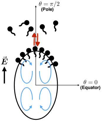
Figure 1: Sketch of the problem: A leaky dielectric viscous drop immersed in another dielectric fluid, with an external electric field $\vec{\textbf{E}}$ in the $z$ direction. The bead-rod particles represent insoluble and bulk surfactants. The double arrows denote adsorption-desorption kinetics while the curved arrows represent the induced flow.

We consider a viscous drop immersed in a leaky dielectric fluid in the presence of surfactants and subject to an electric field, as shown in figure 1. Each fluid is characterized by the fluid viscosity $\mu$, dielectric permittivity $\varepsilon$, and conductivity $\sigma$ with the superscript denoting interior (-) or exterior (+) fluid. In this work we denote the contrasts of those properties by $\mu_{r}=\mu^{+}/\mu^{-}$, $\varepsilon_{r}=\varepsilon^{-}/\varepsilon^{+}$, and $\sigma_{r}=\sigma^{+}/\sigma^{-}$.

II.1 Formulation

The fluids are governed by the incompressible Stokes equations, neglecting inertia

$$-\nabla p+\mu\nabla^{2}\bm{u}+\bm{F}=\bm{0},$$ (2)

where $p$ and $\bm{u}$ are the pressure and velocity field, respectively; $\bm{F}$ is a singular force defined at the drop surface, as described below. The electric field $\textbf{E}=-\nabla\phi$, where $\phi$ is the electric potential that satisfies the Laplace equation both inside and outside the drop in the extended leaky dielectric model,

$$\nabla^{2}\phi=0.$$ (3)

The surfactant transport on the drop surface and in the exterior bulk fluid are described by the following set of coupled equations

$$\dfrac{\partial\Gamma}{\partial t}+\nabla_{s}\cdot\left(\Gamma\bm{v}_{s}\right)+\Gamma(\nabla_{s}\cdot\bm{n})\bm{u}_{s}\cdot\bm{n} =D_{s}\nabla_{s}^{2}\Gamma+\beta C_{s}\left(\Gamma_{\infty}-\Gamma\right)-\alpha\Gamma,$$ (4)

$$\dfrac{\partial C}{\partial t}+\bm{u}\cdot\nabla C =D\nabla^{2}C,$$ (5)

where $\bm{n}$ is the normal vector, $\bm{u}_{s}$ is the surface velocity on the drop and $\bm{v}_{s}=(I-\bm{n}\bm{n})\bm{u}_{s}$ is the velocity tangential component along the drop. $\Gamma$ and $C$ are the surfactant concentration on the drop surface and in the bulk, respectively; $C_{s}$ is the concentration of surfactant in the fluid immediately adjacent to the drop surface; $\alpha$ and $\beta$ are the kinetic constants for desorption and adsorption, respectively; $D_{s}$ and $D$ are the diffusion constant on the drop surface and in the bulk correspondingly.

At the drop interface, boundary conditions are imposed for the electric potential $\phi$, the flow field $\bm{u}$, and the bulk surfactant concentration $C$. First, the electric potential is continuous and the total current is conserved,

$$\llbracket\phi\rrbracket=0,\quad\underbrace{\llbracket\sigma\nabla\phi\cdot\bm{n}\rrbracket}_{\text{Ohmic current}}=\underbrace{\frac{d\tilde{q}}{dt}}_{\text{Charge relaxation}}+\underbrace{\nabla_{s}\cdot(\tilde{q}\bm{u}_{s})}_{\text{Charge convection}},$$ (6)

where $\tilde{q}=-\llbracket\varepsilon\nabla\phi\cdot\bm{n}\rrbracket$ represents the surface charge density, and $\llbracket\cdot\rrbracket$ denotes the jump between outside and inside quantities. The effects of charge relaxation on the transient behavior of drop (Lanauze et al., 2013), and of convection on equilibrium deformation (Lanauze et al., 2015; Das and Saintillan, 2017a, b), have been investigated analytically and numerically in the context of drops electrohydrodynamics. In the present study, we neglect these effects to more easily isolate the surfactant effects. This reduces Eq. 6 to only consider the Ohmic current:

$$\llbracket\phi\rrbracket=0,\quad\llbracket\sigma\nabla\phi\cdot\bm{n}\rrbracket=0.$$ (7)

Second, the electric and fluid problems are coupled through the stress balance

$$\underbrace{\llbracket-p+\mu\left(\nabla\bm{u}^{T}+\nabla\bm{u}\right)\rrbracket}_{\text{Hydrodynamic stress}}\cdot\bm{n}+\underbrace{\llbracket\varepsilon\left(\bm{E}\bm{E}-\frac{1}{2}(\bm{E}\cdot\bm{E})\mathbf{I}\right)\rrbracket}_{\text{Electric stress}}\cdot\bm{n}=\underbrace{\gamma(\nabla_{s}\cdot\bm{n})\bm{n}}_{\text{Surface tension}}-\underbrace{\nabla_{s}\gamma}_{\text{Marangoni stress}}.$$ (8)

Surfactants act to lower the surface tension, which now depends on the concentration of surfactants through the equation of state Eq. 1. As a result, the non-uniform surfactant distribution induced by the flow in and around the drop yields a surface tension gradient (the Marangoni stress).

Finally, to close the system we need a third boundary condition that describes the flux of surfactants between the surface of the drop and and the bulk. The interfacial condition for the surfactant concentration,

$$D\bm{n}\cdot\nabla C=\beta C_{s}\left(\Gamma_{\infty}-\Gamma\right)-\alpha\Gamma,$$ (9)

where $\bm{n}\cdot\nabla C=\partial C/\partial\bm{n}$ denotes the normal derivative of $C$. We henceforth concentrate on axisymmetric solutions only.

II.2 Nondimensionalization

In this work we set the exterior fluid viscosity equal to the interior fluid viscosity: $\mu^{+}=\mu^{-}=\mu$. We use the drop size $r_{0}$ to scale length, capillary pressure $\gamma_{0}/r_{0}$ to scale pressure, equilibrium surfactant concentration $\Gamma_{eq}$ to scale $\Gamma$, the far-field surfactant concentration $C_{\infty}$ to scale the bulk surfactant concentration, and electrically driven flow $U_{d}=\varepsilon^{+}E_{0}^{2}r_{0}/\mu$ to scale velocity, in which $E_{0}$ denotes the intensity of the external electric field.

There are nine dimensionless physical parameters that characterize this system: (1) the electric capillary number $\text{Ca}_{E}\equiv\mu U_{d}/\gamma_{eq}=\varepsilon^{+}E_{0}^{2}r_{0}/\gamma_{eq}$ (ratio of electric pressure to capillary pressure), (2) permittivity ratio $\varepsilon_{r}=\varepsilon^{-}/\varepsilon^{+}$, (3) conductivity ratio $\sigma_{r}=\sigma^{+}/\sigma^{-}$, (4) the elasticity constant $E=RT\Gamma_{\infty}/\gamma_{0}$ in the Langmuir equation of state, (5) the surfactant coverage $\chi=\Gamma_{eq}/\Gamma_{\infty}$, (6) the insoluble surfactant Péclet number $\text{Pe}_{s}=r_{0}U_{d}/D_{s}$, (7) the bulk surfactant Péclet number $\text{Pe}=r_{0}U_{d}/D$, (8) the transfer parameter $J=C_{\infty}D/\Gamma_{eq}U_{d}$ and (9) the Biot number $\text{Bi}=\alpha\tau_{EHD}$ (ratio of EHD characteristic time scale to desorption time scale).

The elasticity number $E$ measures the sensitivity of the surface tension to the surface surfactant concentration, whereas in the presence of surfactant exchange between the bulk and the drop interface, the surfactant coverage is related to the adsorption constant $k=\beta C_{\infty}/\alpha$ in Eq. 10Chen and Stebe (1996); Eggleton and Stebe (1998)

$$\chi=\dfrac{k}{k+1}.$$ (10)

The bulk and surface Péclet numbers denote the relative strength of convective transport versus diffusive transport. These two numbers also represent the ratio of two time scales: $\text{Pe}=\tau_{D}/\tau_{EHD}$, where $\tau_{EHD}=r_{0}/U_{d}$ is the EHD flow time scale, and $\tau_{D}=r_{0}^{2}/D$ is the surfactant diffusion time scale. The parameter $J$ gives a measure of transfer of surfactant between its bulk and adsorbed forms relative to advection on the interface. It is important to note the ratio $\text{Bi}/J$ distinguishes two types of transport regime (Chang and Franses, 1995; Wang et al., 2014): diffusion-controlled transport ($\text{Bi}/J>1$), and sorption-controlled transport ($\text{Bi}/J\ll 1$). In terms of the above dimensionless parameters, the clean drop cases correspond to $E=0$ or $\chi=0$ (Eq. 15). The case of insoluble surfactants corresponds to $\text{Bi}=0$ (Eq. 16c). The non-diffusive case corresponds to $\text{Pe},\text{Pe}_{s}\gg 1$.

We obtain the following dimensionless equations

$$-\nabla p+\text{Ca}\nabla^{2}\bm{u}+\bm{F} =\bm{0},$$ (11)

$$\nabla^{2}\phi =0,$$ (12)

$$\dfrac{\partial\Gamma}{\partial t}+\nabla_{s}\cdot\left(\Gamma\bm{v}_{s}\right)+(\nabla_{s}\cdot\bm{n})\bm{u}_{s}\cdot\bm{n}\Gamma =\dfrac{1}{\text{Pe}_{s}}\nabla_{s}^{2}\Gamma+J\bm{n}\cdot\nabla C,$$ (13)

$$\dfrac{\partial C}{\partial t}+\bm{v}\cdot\nabla C =\dfrac{1}{\text{Pe}}\nabla^{2}C,$$ (14)

$$\gamma =1+E\ln(1-\chi\Gamma)$$ (15)

On the drop surface, the dimensionless boundary conditions are given by

$$\llbracket\phi\rrbracket=0,\quad\llbracket\sigma\nabla\phi\cdot\bm{n}\rrbracket=0,$$ (16a)

$$\llbracket-p+\text{Ca}\left(\nabla\bm{u}^{T}+\nabla\bm{u}\right)\rrbracket\cdot\bm{n}+\llbracket\text{Ca}_{E}\left(\bm{E}\bm{E}-\frac{1}{2}(\bm{E}\cdot\bm{E})\mathbf{I}\right)\rrbracket\cdot\bm{n}=\gamma(\nabla_{s}\cdot\bm{n})\bm{n}-\nabla_{s}\gamma,$$ (16b)

$$J\bm{n}\cdot\nabla C=\text{Bi}\left[C_{s}\left(1+k-k\Gamma\right)-\Gamma\right].$$ (16c)

In Eq.11 and Eq. 16b the capillary number $\text{Ca}=\mu U_{d}/\gamma_{0}$ is the ratio of electric stress to tension in the absence of surfactant.

The singular force

$$\bm{F}=\int_{0}^{2\pi}\left(\bm{f}_{\gamma}+\text{Ca}_{E}\bm{f}_{E}\right)\delta^{2}\left(\bm{x}-\bm{X}(s,t)\right){\rm~{}d}s,$$ (17)

where the electric force

$$\bm{f}_{E}=\llbracket\varepsilon\left(\bm{E}\bm{E}-\frac{1}{2}(\bm{E}\cdot\bm{E})\mathbf{I}\right)\rrbracket\cdot\bm{n},$$

and the surface tension force

$$\bm{f}_{\gamma}=\nabla_{s}\gamma-\gamma(\nabla_{s}\cdot\bm{n})\bm{n}.$$

The right-hand side of the stress balance Eq. 16b shows that two surfactant-related mechanisms govern the deformation of drops. The first one is due to the non-uniform surfactant distribution that affects the surface tension. This mechanism acts in the normal direction, and is further broken down into two phenomena: tip-stretching and surface dilution (Pawar and Stebe, 1996). A measure of tip-stretching is the local surface tension for which $\gamma<1$ indicates larger deformation. The area-average surface tension $\gamma_{\text{avg}}$ gives a global measure of the dilution effect; smaller deformations are attained for $\gamma_{\text{avg}}>1$. The second mechanism is driven by the Marangoni stress, which acts to suppress (Pawar and Stebe, 1996; Weidner, 2013) or even reverse (Weidner, 2013) surface convective fluxes. The Marangoni stress acts in the tangential directions, and consists of two principal components: the derivative of surface tension as a function of surfactant concentration ($\partial\gamma/\partial\Gamma$) and the surfactant concentration gradient ($\partial\Gamma/\partial\theta$), where $\theta$ is the angle parameter.

These nontrivial and highly nonlinear mechanisms pose challenges in studying the EHD of a surfactant-laden viscous drop. Analytical solutions of the transport equation are only possible in very restricted limits (Kallendorf et al., 2015), and often numerical simulations are necessary. Several computational methods have been developed to simulate surfactants effects on droplets (Muradoglu and Tryggvason, 2008; Lai et al., 2011; Xu et al., 2014, 2018). In the context of EHD, we refer the readers to the results in (Teigen and Munkejord, 2010; Lanauze et al., 2018; Sorgentone and Tornberg, 2018).

In this work we implement a numerical code based on the immersed interface method (IIM) integrating numerical tools developed by our group Nganguia et al. (2015, 2016); Hu et al. (2018). A description of the numerical setup is provided in A, together with numerical validation in B and convergence study in C.

Moreover we fix the viscosity ratio $\mu_{r}=1$, the elasticity constant $E=0.2$ and conduct simulations with various combinations of parameters to investigate the effects of surfactant solubility on the drop electrohydrodynamics. Our simulations show that deformation and flow patterns appear to be invariant with increasing surfactant solubility when the surfactant coverage $\chi<0.8$. We therefore focus our analysis on elevated surfactant coverage with $\chi=0.9$. This surfactant coverage is in the relevant range in many experimental setups Ha and Yang (1995, 1998); Anna and Mayer (2006), and the corresponding (dimensionless) surface tension $\gamma_{eq}=1+E\ln(1-\chi)=0.54$ and adsorption number $k=\chi/(1-\chi)=9$. The Péclet numbers $\text{Pe}=\text{Pe}_{S}=100$ for the oblate shapes (§ III.3) and $\text{Pe}=\text{Pe}_{S}=500$ for the prolate shapes (§ III.1 and § III.2). These values of the Péclet numbers correspond to transfer parameter $J\ll 1$; specifically $J=2\times 10^{-3}$ for the prolate cases, and $J=10^{-2}$ for the oblate cases. This limit corresponds to the diffusion-controlled surfactant transport that is relevant in many practical applications (Wang et al., 2014). Finally in § IV we investigate the effect of solubility at larger values of $J$.

III Effects of surfactant physico-chemistry on drops electrohydrodynamics: $J\ll 1$

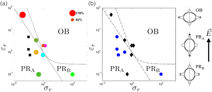
Figure 2: $\sigma_{r}$–$\varepsilon_{r}$ phase plane depicting regions of prolate ‘A’, prolate ‘B’, and oblate drop shapes. The drops on the right-hand side depicts the expected circulation for each shape: counterclockwise (in the first quadrant) for the prolate ‘A’, and clockwise for the prolate ‘B’ and oblate shapes. (a) Solubility effect on deformation: ($\blacksquare$) indicates instability due to solubility, and the colored ($\bigcirc$) represent the relative change in deformation between clean and soluble drops. Larger sized circle point to greater solubility effect on deformation. (b) Solubility effect on flow: The symbols denote the effects of surfactant solubility for a given $(\sigma_{r},\varepsilon_{r})$ pair on the flow in and around the drop: ( ) denotes a qualitative change in flow (reversal or stagnation point), and ($\mathop{\raisebox{-1.06558pt}{$\leavevmode\hbox to5.04pt{\vbox to7.56pt{\text{[drawing]}}}$}}$) represents no change in flow compared to the clean case. The electric capillary number $\text{Ca}_{E}=0.25$, and the transfer parameter $J=10$.

The shape of a viscous drop under an electric field can be either prolate or oblate: A prolate shape is when a drop elongates along the applied electric field, while an oblate shape is when a drop elongates in the orthogonal direction to the electric field. Prolate drops are further categorized as ‘A’ and ‘B’, distinguished by the circulation patterns inside the drop: counterclockwise (equator-to-pole) for prolate ‘A’, and clockwise (pole-to-equator) for prolate ‘B.’ The oblate shape is characterized by a clockwise circulation (pole-to-equator).

Figure 2 shows the phase diagram for the prolate versus oblate drops in the $(\sigma_{r},\varepsilon_{r})$ plane. The dashed curves are boundaries for a clean (surfactant-free) viscous drop (see Lac and Homsy (2007) and references therein). These boundaries are affected by insoluble surfactants (Nganguia et al., 2013), and this is corroborated by our current simulation results. Symbols in figure 2 are parameters collected from the literature.

Table 2: Surfactant effects at surfactant coverage $\chi=0.9$ and $J=10$. The circulation in the first quadrant is is either clockwise (C), counterclockwise (CC), or features a stagnation point (S) with eddies.

$\sigma_{r}$	$\varepsilon_{r}$	Refs.	I (clean)	II (insoluble)	III (soluble)
0.33	1	(Teigen and Munkejord, 2010)	CC	C, stable	CC, stable
0.33	3.5	(Teigen and Munkejord, 2010)	C	C, stable	C, stable
1	2	(Teigen and Munkejord, 2010)	C	C, stable	C, stable
0.1	5	(Lac and Homsy, 2007)	CC	C, stable	CC, unstable
0.04	50	(Lac and Homsy, 2007)	C	C, unstable	C, stable
100	0.1	(Lac and Homsy, 2007)	C	S, unstable	C, stable
0.1	1.37	(Lac and Homsy, 2007; Ha and Yang, 2000a)	CC	S, stable	CC, unstable
0.97	0.75	(Lanauze et al., 2018)	CC	CC, stable	CC, stable
0.125	0.75	(Lanauze et al., 2018)	CC	S, stable	CC, unstable
1.33	2	(Mandal et al., 2016b)	C	C, stable	C, stable

We use these parameters to study the effects of surfactant solubility by drawing direct comparison with results for a clean drop.

We summarize the solubility effects on drop deformation (with Bi=10) in figure 2a, where the size of each circle correlates with the relative increase in deformation between surfactant-covered and clean drops (with the smallest and the largest sizes in the legend). Filled squares ($\blacksquare$) are for parameters where surfactant solubility gives rise to instability and the equilibrium shape (which exists for a clean drop) no longer exists.

We summarize the solubility effects on the flow in figure 2b, where the filled diamonds ($\mathop{\raisebox{-1.18399pt}{$\leavevmode\hbox to5.6pt{\vbox to8.4pt{\text{[drawing]}}}$}}$) denote parameters where the flow around a surfactant-laden drop is qualitatively similar to the circulation pattern of a clean drop with the same parameters. The blue circles represents parameters where the flow pattern is qualitatively changed by solubility. For example, the flow inside a ( ) drop with $(\sigma_{r},\varepsilon_{r})=(0.1,5)$ changes from a counterclockwise circulation (prolate ‘A’) to a clockwise circulation (prolate ‘B’) due to insoluble surfactant, then changes to a configuration of two counter rotating vortices due to surfactant solubility as shown in figure 3.

Table 2 summarizes the dynamics observed for each set of parameters. Column I is for the shape (circulation) of a clean drop: prolate ‘A’ (counterclockwise, CC), prolate ‘B’ (clockwise, C), and oblate (clockwise) (also see figure 2). Columns II and III are for the circulation inside a drop covered with insoluble surfactant ($\text{Bi}=0$) and soluble surfactant ($\text{Bi}=10$), respectively. Also in these two columns we indicate whether an equilibrium shape is attained (stable) or not (unstable) in the presence of insoluble (II) or soluble (III) surfactants at sufficiently high electric capillary number.

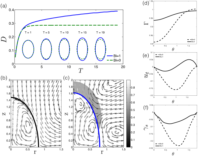
Figure 3: A prolate drop with $(\sigma_{r},\varepsilon_{r})=(0.1,5)$ and electric capillary number $\text{Ca}_{E}=0.25$. (a) Deformation as a function of dimensionless time $T$ with Biot numbers $\text{Bi}=0$ (insoluble case) and $\text{Bi}=1$. The inset shows the drop shapes at various times. (b&c) Flow field at $T=19$ for Biot number $\text{Bi}=0$ (b), and $\text{Bi}=1$ (c). (d) Surfactant distribution, (e) tangential velocity $u_{t}=\bm{v}_{s}\cdot\bm{t}$, and (f) Marangoni stress as a function of $\theta$, with the solid (dashed) curves for $\text{Bi}=0$ ($\text{Bi}=1$). In (c), the surfactant sorption kinetics is found to be adsorption, color-coded by the blue on the drop surface.

Below we elucidate the detailed solubility effects on the EHD of a viscous drop. Our simulations show that surfactant effects are quite similar in regions of $(\sigma_{r},\varepsilon_{r})$ for prolate ‘B’ and oblate clean drop. Thus we focus on regions where the clean drop is either prolate ‘A’ or oblate.

III.1 Increasing Biot number destabilizes a prolate drop

Here we show that enhancing the surfactant solubility (by increasing Biot number) renders a prolate drop unstable. Specifically we use the combination $(\sigma_{r},\varepsilon_{r})=(0.1,5)$, where a surfactant-free viscous drop is prolate ‘A’ under an electric field. For a clean drop with $(\sigma_{r},\varepsilon_{r})=(0.1,5)$ the steady equilibrium prolate ‘A’ drop exists at all values of $\text{Ca}_{E}$ (Lac and Homsy, 2007), whereas we establish equilibrium drop shape exists for the insoluble surfactant case up to $\text{Ca}_{E}=0.3$. Figure 3a shows the transient deformation number as a function of dimensionless time $T$ for a prolate drop with $\text{Ca}_{E}=0.25$ and $\text{Bi}=1$. Starting from a spherical drop covered with a uniform surfactant distribution both on the drop interface and in the bulk, we simulate the drop EHD and examine the flow field, surfactant distribution, and the drop deformation number defined as

$$D=\frac{L-B}{L+B},$$ (18)

where $L$ is the length of the major axis and $B$ is the length of the minor axis of the ellipsoid.

When the surfactant is insoluble ($\text{Bi}=0$) and weakly-diffusive (Peclet number $\text{Pe}_{S}\gg 1$), the drop first elongates along the electric field with a flow from the equator to the pole, moving the surfactant from the equator to pole. As the surfactant accumulates and builds up the Marangoni stress, the flow is reversed (from pole to equator) around $T\sim 0.6$ and the drop reaches a equilibrium prolate shape with a clockwise circulation after $T\sim 4$ in figure 3 in figure 3b. This circulation at equilibrium is opposite to that of a clean prolate ‘A’ drop, and the flow magnitude is much smaller: The Marangoni stress due to the non-diffusive insoluble surfactant changes the circulation from counter-clockwise (prolate ‘A’ for the clean drop) to clockwise (prolate ‘B’).

However, as we increase the Biot number to allow for more surfactants exchange between the bulk and the surface of the drop, we find that the steady state no longer exists as the drop continuously deforms until the end of simulations (up to $T=20$) as illustrated in figure 3a. The surfactant distribution $\Gamma$, tangential velocity $\bm{u}_{t}$ and the Marangoni stress $\gamma_{s}$ at $T=20$ are plotted in figures 3d, e and f, respectively.

For the case of insoluble surfactant ($\text{Bi}=0$) in figure 3b, the Marangoni stress is able to sustain an equilibrium shape. In the simulations as we gradually increase the surfactant exchange between the bulk and the drop surface (by increasing Bi from zero), we find that the Marangoni stress is reduced in magnitude (figure 3f) because the surfactant on the drop surface is homogenized (figure 3d) by the adsorption/desorption of surfactant.

Figure 3e shows the corresponding tangential velocity on the drop interface. We observe that the surfactant solubility not only reduces the magnitude of the tangential velocity but also gives rise to the development of counter rotating eddies inside the drop, as shown in figure 3c. Such counter rotating eddies inside a viscous drop are also observed in a clean viscous drop elongating indefinitely under a DC electric field Lac and Homsy (2007).

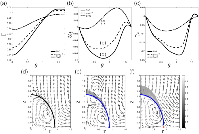
Figure 4: A prolate drop with $(\sigma_{r},\varepsilon_{r})=(1/3,1)$ and $\text{Ca}_{E}=0.3$. (a) Surfactant distribution, (b) tangential velocity $u_{t}=\bm{v}_{s}\cdot\bm{t}$, and (c) Marangoni stress as a function of $\theta$. $\text{Bi}=0$ for solid curves, $\text{Bi}=10^{-2}$ for dashed curves, and $\text{Bi}=10$ for dash-dotted curves. (d-f) Corresponding flow fields for (d) $\text{Bi}=0$, (e) $\text{Bi}=10^{-2}$ and (f) $\text{Bi}=10$. In (e)-(f), the drop surface is color-coded to represent sorption kinetics: blue for adsorption, and red for desorption.

III.2 Effects of Biot number on flow around a prolate drop

In § III.1 the surfactant solubility affects both drop deformation and the flow pattern of a prolate drop. Here we investigate another scenario where the surfactant solubility affects only the flow pattern while the equilibrium drop shape remains close to the prolate shape of a drop covered with insoluble surfactants under an electric field. Specifically we focus on the combination $(\sigma_{r},\varepsilon_{r})=(1/3,1)$ with $\text{Ca}_{E}=0.3$. Simulations show that the equilibrium drop deformation is minimally influenced by surfactant solubility at all values of the electric capillary number (with the change in deformation less than 1% between the insoluble case and $\text{Bi}=10$) because sorption kinematics induce little change in the total amount of surfactant as shown in figure 5a (solid curve). Consequently the average surface tension does not vary much with Bi, leading to little change in drop deformation with increased surfactant solubility.

The flow pattern, on the other hand, is highly dependent on the surfactant distribution and kinetics. Without surfactant the clean drop is prolate ‘A’ at equilibrium with a counterclockwise flow under an electric field. For $\text{Bi}=0$ the transport of an insoluble surfactant and the corresponding Marangoni stress gives rise to an interior flow dominated by a clockwise circulation with a small-counter rotating eddy around the pole as shown in figure 4d, and the corresponding tangential velocity is shown in figure 4b. As the Biot number is increased to $\text{Bi}=10^{-2}$ the counterclockwise eddy near the pole expands as shown in figure 4e, with the corresponding tangential velocity in figure 4b.

When we further increase the Biot number ($\text{Bi}=10$), the counterclockwise eddy nearly takes over the whole interior flow (figure 4f) as the surfactant is nearly constant (dash-dotted curve in figure 4a) and the Marangoni stress is of the smallest magnitude in figure  4f. This can be explained by examining the surface tension derivative and surfactant gradient. The former remains high, and strong Marangoni stresses are realized initially. However, adsorption dominates the surfactant exchange, and the surfactant distribution remains nearly uniform. This results in decreasing surfactant gradient, and therefore smaller overall Marangoni stress at equilibrium.

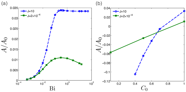
Figure 5: A prolate drop with $(\sigma_{r},\varepsilon_{r})=(1/3,1)$ and $\text{Ca}_{E}=0.3$. (a) Change in total amount $A$ of adsorbed surfactant for the prolate drop in §III.2 with an initial bulk concentration $C_{0}=1$. (b) Change in total surfactant as a function of the initial bulk surfactant concentration, $C_{0}$. The Biot number $\text{Bi}=1$.

To further examine how sorption/desorption of surfactant affects the drop deformation and flow pattern, we study the surfactant transport and distribution as follows. First we investigate the total amount of adsorbed surfactant $A$, defined as the difference in total amount of surfactant on the drop surface between the time $T$ and the initial time 0:

$$A\equiv A_{T}-A_{0}\equiv\int\Gamma(T){\rm~{}d}s-\int\Gamma(0){\rm~{}d}s.$$ (19)

Using this definition, $A>0$ denotes adsorption, and $A<0$ represents desorption.

Figure 5a shows the total amount of adsorbed surfactant $A$ as a function of Biot number, for the prolate drop in §III.2. For an initial bulk surfactant concentration equals to the concentration in the far field, $A$ exhibits a non-monotonic behavior with a critical Biot number $\text{Bi}_{\text{cr}}\approx 0.3$, where the adsorbed surfactant concentration is maximized. Moreover, we observe that adsorption ($A>0$) is the dominant kinetics for the full range of Biot number studied. Our simulations show this result is strongly dependent on the initial bulk surfactant concentration $C_{0}$. As illustrated in figure 5b that shows the total amount of adsorbed surfactant as a function of initial surfactant concentration in the bulk, desorption ($A<0$) becomes the dominant kinetics as $C_{0}$ is reduced.

Finally the stagnation point between two counter rotating eddies observed here are similar to those observed for multi-lobed, prolate-shaped clean drops Lac and Homsy (2007). However, and unlike the case of clean drops in Lac and Homsy (2007), we hypothesize the flow reversal and eddies formation are driven by competition between the electrically-induced and Marangoni flows, possibly in similar manner as reported in previous findings on surfactant-laden liquid films under gravity Weidner (2013).

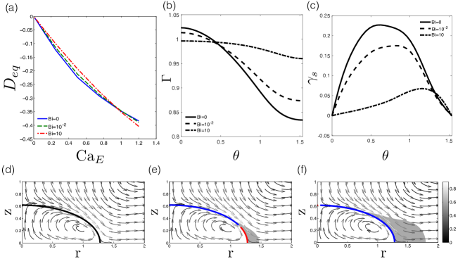
Figure 6: An oblate drop with $(\sigma_{r},\varepsilon_{r})=(1,2)$. (a) Deformation number as a function of $\text{Ca}_{E}$. (b) Surfactant distribution, and (c) Marangoni stress as a function of $\theta$. Solid lines are for $\text{Bi}=0$ (the insoluble surfactant case), dashed lines are for $\text{Bi}=10^{-2}$, and dash-dotted lines are for $\text{Bi}=10$. (d-f) Flow field at $\text{Ca}_{E}=1$ for Biot number $\text{Bi}=0$ (d), $\text{Bi}=10^{-2}$ (e), and $\text{Bi}=10$ (f). In (d-f) the drop surface is color-coded to represent sorption kinetics: blue for adsorption, and red for desorption.

III.3 Effects of Biot number on equilibrium deformation of an oblate drop

Here we consider the combination $(\sigma_{r},\varepsilon_{r})=(1,2)$ that corresponds to a surfactant-laden oblate drop (with and without surfactant solubility). The equilibrium deformation shows a visible dependence on both the electric capillary and Biot numbers, as illustrated in figure 6a. The deformation undergoes a transition around $\text{Ca}_{E}\approx 1$: The absolute deformation is smaller at low to moderate electric field strength compared to the insoluble case, while increasing the Biot number yields larger deformation at electric capillary numbers $\text{Ca}_{E}>1$.

Figures 6b&c show the surfactant distribution and Marangoni force as a function of $\theta$ at $\text{Ca}_{E}=1$. The corresponding flow field and the bulk surfactant distribution are in figures 6d ($\text{Bi}=0$), 6e ($\text{Bi}=10^{-2}$), and 6f ($\text{Bi}=10$). For $(\sigma_{r},\varepsilon_{r})=(1,2)$ we find that the interior flow remains a clockwise circulation (from pole to equator) for all values of the Biot number.

Locally at the equator ($\theta=0$), the surface tension is less than $\gamma_{eq}$ for insoluble and weak surfactant exchange, suggesting that tip-stretching dominates. However, at higher Biot number the surface tension at the equator is slightly greater than $\gamma_{eq}$. Looking at sorption kinetics, adsorption dominates but for a region of desorption near the equator ($\text{Bi}=10^{-2}$ in figure 6e), while adsorption dominates on the entire drop surface for strong surfactant exchange ($\text{Bi}=10$ in figure 6f). In terms of surface dilution, the average surface tension $\gamma_{\text{avg}}$ remains less than unity with increasing Biot number. This couples with the local surface tension at the equator that is above $\gamma_{eq}$, suppressing deformation.

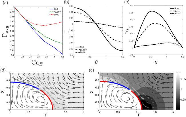
Figure 7: An oblate drop with $(\sigma_{r},\varepsilon_{r})=(1,2)$. (a) Average surfactant concentration as a function of $\text{Ca}_{E}$. (b) Surfactant distribution, and (c) Marangoni stress as a function of $\theta$ at $\text{Ca}_{E}=0.5$. Solid lines are for $\text{Bi}=0$ (the insoluble surfactant case), dashed lines are for $\text{Bi}=10^{-2}$, and dash-dotted lines are for $\text{Bi}=10$. (d-e) Flow field at $\text{Ca}_{E}=0.5$ for Biot number $\text{Bi}=10^{-2}$ (d) and $\text{Bi}=10$ (e). In (d-e) the drop surface is color-coded to represent sorption kinetics: blue for adsorption, and red for desorption.

Figure 7a shows the average surfactant $\Gamma_{\text{avg}}$ as a function of $\text{Ca}_{E}$. The rise of $\Gamma_{\text{avg}}$ for $\text{Ca}_{E}>0.8$ for $\text{Bi}=10$ corresponds to a reduced capillary pressure associated with the enhanced drop deformation in figure 6a. Figure 7b&c show the surfactant distribution and Marangoni stress at $\text{Ca}_{E}=0.5$, and the corresponding flow field in figure 7d ($\text{Bi}=10^{-2}$) and figure 7e ($\text{Bi}=10$).

IV Effects of surfactant physico-chemistry on drops electrohydrodynamics: $J>1$

As we specified earlier, the ratio $\text{Bi}/J$ differentiates between diffusion-controlled transport ($\text{Bi}/J>1$), and sorption-controlled transport ($\text{Bi}/J\ll 1$). In the previous section we focus on the diffusion-controlled regime. Here we focus on the sorption-controlled regime (with $J=10$) and make comparison with results for the diffusion-controlled regime in §III.

IV.1 Unstable drop dynamics

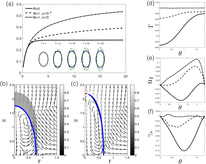
Figure 8: A prolate drop with $(\sigma_{r},\varepsilon)=(0.1,5)$ and $\text{Ca}_{E}=0.25$. (a): Drop shapes for the prolate drop. (b) and (c): Flow field at $T=19$ for $J=10^{-3}$ (b) and $J=10$ (c) with $\text{Bi}=1$. (d): Surfactant distribution, (e): tangential velocity $u_{t}=\bm{v}_{s}\cdot\bm{t}$, and (f): Marangoni stress. The solid lines are for $\text{Bi}/J=0$. The dashed and dash-dotted lines are for $\text{Bi}=1$ with $J=10^{-3}$ and $J=10$, respectively. In (b-c) the drop surface is color-coded to represent sorption kinetics: blue for adsorption, and red for desorption.

First we focus on the prolate drop with $(\sigma_{r},\varepsilon_{r})=(0.1,5)$ (§III.1) and make comparison between $J=10^{-3}$ (figure 3) and $J=10$ with $\text{Bi}=1$. Figure 8a shows the drop shape from $T=1$ to $T=19$. Figure 8b&c are the corresponding flow field at $T=19$ with $J=10^{-3}$ and $J=10$, respectively.

For insoluble surfactants ($\text{Bi}/J=0$, solid curves in figure 8a, d, e & f), the surfactant has the most spatial inhomogeneity that corresponds to a large Marangoni stress. With soluble surfactant in the diffusion-controlled regime ($\text{Bi}/J>1$, dashed curves) the surfactant sorption kinetics greatly reduces the Marangoni stress, giving rise to larger drop deformation. In the sorption-controlled regime ($\text{Bi}/J=0.1<1$, dash-dotted curves) the surfactant concentration $\Gamma$ is nearly homogeneous and the Marangoni stress is quite small, corresponding to the largest and fastest deformation in (a). We note that suppressing the Marangoni stress in the diffusion-controlled regime gives rise to a $25\%$ increase in drop deformation (compared to the insoluble case), while in the sorption-controlled regime a $60\%$ increase in drop deformation is found in the simulations.

Finally we observe that for the sorption-controlled case, the surfactant kinetics at the drop tip ($\theta=\pi/2$ in figure 8c) is dominated by desorption (red portion of the drop surface in figure 8c) while for the diffusion-controlled case the surfactant kinetics is dominated by adsorption all over the drop (see blue portion of the drop surface in figure 3c). However, the total amount of surfactant increases on the drop surface for both cases.

IV.2 Transient overshoot and equilibrium drop dynamics

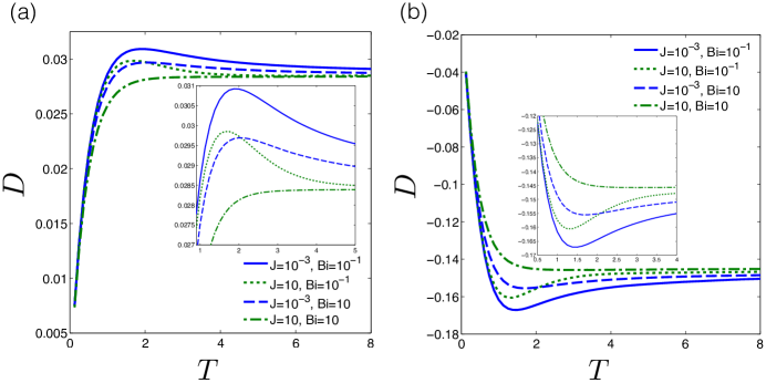
Figure 9: Deformation as a function of dimensionless time $T$ for (a) a prolate drop with $(\sigma_{r},\varepsilon)=(0.97,0.75)$, and (b) the oblate drop with $(\sigma_{r},\varepsilon_{r})=(4/3,2)$. $\text{Ca}_{E}=0.25$ for both cases. The solid and dotted lines are for low ($J=10^{-3}$), and high ($J=10$) transfer parameter with $\text{Bi}=10^{-1}$, respectively. The dashed and dash-dotted lines represent higher Biot number ($\text{Bi}=10$) with $J=10^{-3}$ and $J=10$, respectively.

In our simulations we observe that the transient dynamics of drop deformation depends on $J$: Figure 9 shows that, at a given value of Bi, the drop deformation number $D$ displays an overshoot en route to the equilibrium for small $J$. Such overshoot in the drop deformation is found for weakly diffusive insoluble surfactant (Nganguia et al., 2019). However, as shown in figure 9 (see inset for close-up of the transient overshoot), the transient overshoot dynamics is suppressed at large $J$: In this case, the deformation monotonically reaches its equilibrium value. We note these observations are valid for both prolate (figure 9a) or oblate (figure 9b) drops.

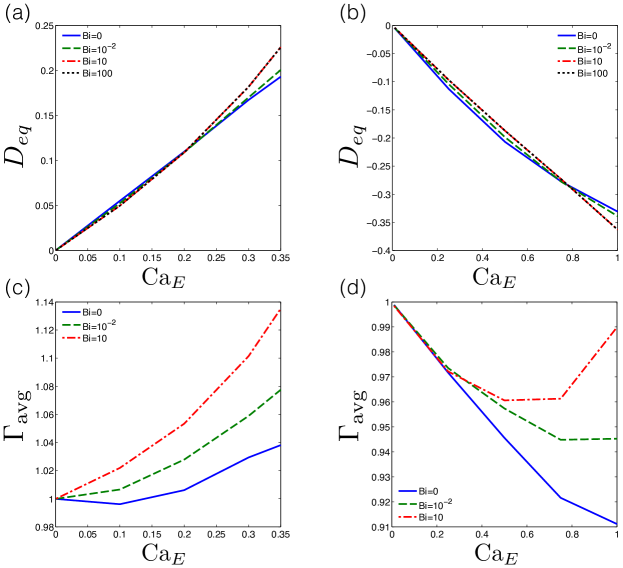
Figure 10: Equilibrium drop deformation and average surfactant coverage as a function of electric capillary number $\text{Ca}_{E}$ for four values of Bi (as labeled) and $J=10$. (a) and (c): a prolate drop with $(\sigma_{r},\varepsilon)=(1/3,1)$. (b) and (d): an oblate drop with $(\sigma_{r},\varepsilon_{r})=(1,2)$.

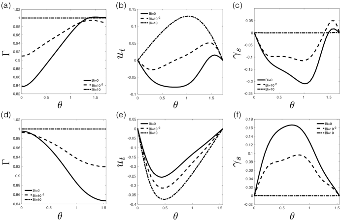
Figure 11: Surfactant distribution (first column), tangential velocity ($u_{t}=\bm{v}_{s}\cdot\bm{t}$, second column), and Marangoni force (third column) for a prolate drop (a-c) with $\text{Ca}_{E}=0.35$, and an oblate drop (d-f) with $\text{Ca}_{E}=1$ in figure 10. The corresponding flow fields for each shape and varying Biot numbers are shown in D.

Figure 10 shows the equilibrium deformation as a function of electric capillary number for a prolate drop with $(\sigma_{r},\varepsilon_{r})=(1/3,1)$ (figure 10a) and an oblate drop with $(\sigma_{r},\varepsilon_{r})=(1,2)$ (figure 10b) at $J=10$. Figure 10c&d show the corresponding average surfactant concentration $\Gamma_{\text{avg}}$ versus $\text{Ca}_{E}$. With $J=10$, we expect the Biot number to play a more significant role in the deformation of the drop. This is especially true for the prolate drop, and is reflected in figure 10a. While the drop deformation for a prolate drop in figure 10a does not depend much on Bi for $\text{Ca}_{E}<0.2$, solubility effects become significant for $\text{Ca}_{E}>0.2$. At $\text{Ca}_{E}=0.4$, the equilibrium drop deformation for $\text{Bi}=10$ is more than 20% larger than that of the insoluble case ($\text{Bi}=0$).

For $\text{Bi}\geq 10$ we find that the equilibrium drop deformation does not depend on surfactant solubility again. This is because the surfactant transport transitions from sorption-controlled to diffusion-controlled dynamics as we increase from $\text{Bi}=10^{-2}$ to $\text{Bi}=10$ with $J=10$. In the diffusion-controlled regime, the drop deformation dynamics is discussed in §III (where $J\ll 1$). Once in the sorption-controlled regime $\text{Bi}/J\ll 1$ the surfactant on the drop surface is highly homogenized and thus the deformation is dominated by the balance between the normal Maxwell stress and the normal hydrodynamic stress.

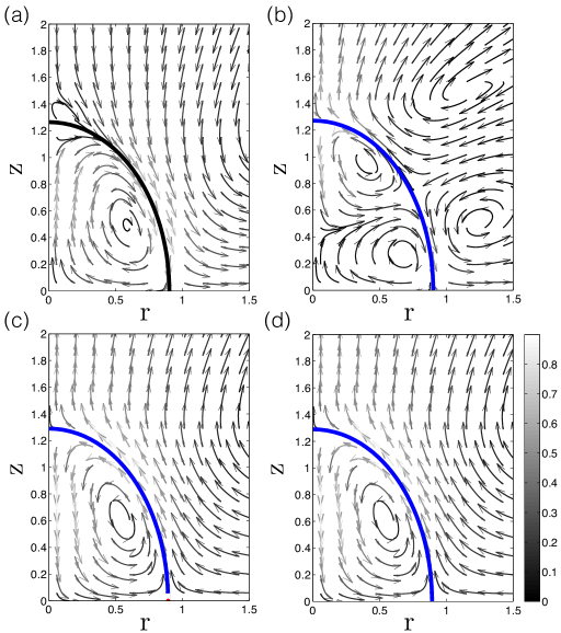
Figure 14: Flow field for a prolate drop in figure 11a-c with $J=10$. The Biot numbers (a) $\text{Bi}=0$, (b) $\text{Bi}=10^{-2}$, (c) $\text{Bi}=10$, and (d) $\text{Bi}=100$. The drop surface is color-coded to represent sorption kinetics: blue for adsorption, and red for desorption.

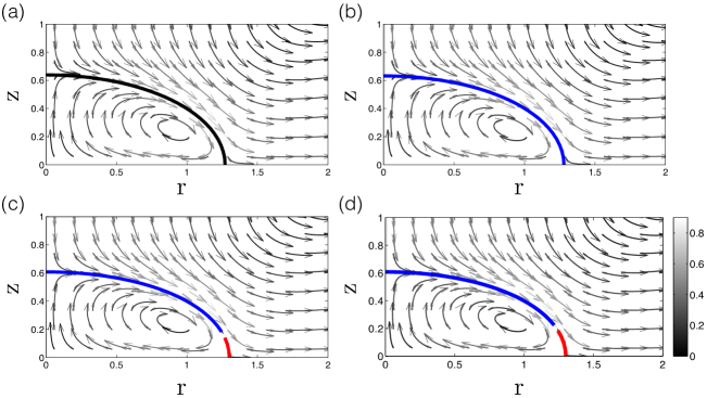
Figure 15: Flow field for the oblate drop in figure 11d-fi with $J=10$. The Biot numbers (a) $\text{Bi}=0$, (b) $\text{Bi}=10^{-2}$, (c) $\text{Bi}=10$, and (d) $\text{Bi}=100$. The drop surface is color-coded to represent sorption kinetics: blue for adsorption, and red for desorption.

In figure 11 we show how Bi affects the spatial variation of the surfactant distribution (a&d), tangential velocity (b&e) and Marangoni stress (c&f) for the two sets of $(\sigma_{r},\varepsilon_{r})$ with $\text{Ca}_{E}=0.35$ for the prolate case and $\text{Ca}_{E}=1$ for the oblate case. Overall we find qualitative similarity in the effects of Bi between $J=10$ and $J\ll 1$ in § III: For a prolate drop (figures 11d, 14), increasing the Biot number transitions the flow from a complete reversal for $\text{Bi}=0$ to development of counter rotating eddits, and then back to its natural prolate ‘A’ circulation for a surfactant-free drop. On the other end, an oblate drop (figures 11e, 15) maintains the same clockwise circulation with increasing Bi.

At high value of the Biot number ($\text{Bi}\geq 10$), figures 11a&d show surfactants are uniformly distributed over the drop surface. In this case, high values of the Biot number and transfer parameter combine to produce uniform surfactant distributions and the drop behaves as if it is a surfactant-free drop with a much reduced surface tension. This is similar to the diffusion-dominated regime ($\text{Pe}_{S}=0$) of a viscous drop covered with insoluble surfactant ($\text{Bi}=0$) (Nganguia et al., 2019).

We also found that at $J=10$ the sorption kinetics depends on the drop shape: Adsorption of surfactant occurs on the surface of a prolate drop (figure 14) while for an oblate drop desorption takes place around the equator (figure 15). This in turn increases the amount of surfactant on the drop surface, as illustrated in figure 11a. Increasing the Biot number leads to a decrease in the surface tension, resulting in a higher deformation with $\approx$25% increase from $\text{Bi}=0$ to $\text{Bi}=10$.

V Conclusion

In the literature many experimental works (Alvarez et al., 2010, 2011, 2012; Sengupta et al., 2019) show that the transport of bulk surfactant is nonlinearly coupled with drop curvature, surfactant physicochemical properties, and external flows. Analytical investigation on drop hydrodynamics with surfactant sorption kinetics is challenging due to the complex nonlinear coupling between surfactant diffusion, sorption kinetics, drop deformation and Maragoni stress. The numerical method in this study provides a useful tool to quantitatively investigate surfactant exchange between the bulk fluid and the drop.

We numerically examined the effect of surfactant solubility on the deformation and circulation of a drop under a dc electric field. In particular we characterize these effects via the dimensionless transfer parameter ($J)$ and Biot number (Bi). We showed that surfactant solubility combines with the electric properties of the fluids in non-trivial ways to produce rich electrohydrodynamics of a viscous drop with $\chi>0.8$.

We first focus on the diffusion-controlled regime in § III. For $(\sigma_{r},\varepsilon_{r})$ that corresponds to a clean prolate ‘A’ drop under an electric field (§ III.1), surfactant solubility affects both the deformation and flow. In most cases explored ( in figure 2b), the presence of insoluble surfactant gives rise to a complete flow reversal (from prolate ‘A’ to prolate ‘B’). Increasing surfactants solubility homogenizes the surfactant distribution on the drop and suppresses the Marangoni stress. In this case we also observe development of stagnation points and counter rotating eddies, with the counterclockwise eddy taking over with increasing Biot number. Results in § III.1 strongly suggest that the critical $\text{Ca}_{E}$ for an equilibrium drop shape depends on the solubility, and we are now investigating how the critical $\text{Ca}_{E}$ depends on various parameters.

For $(\sigma_{r},\varepsilon_{r})$ that corresponds to a clean prolate ‘A’ drop under an electric field (§ III.2), we find that the surfactant solubility does not affect the drop deformation but does affect the flow pattern. In this case (small $J$, moderate Bi and $\text{Ca}_{E}$) we find that the average surface tension does not vary much with the surfactant solubility because there is very little net change in total amount of surfactant due to adsorption/desorption. However the spatial variation in $\Gamma$ is sufficient to induce different flow pattern for the range of electric capillary number we used in the simulations. We are now investigating if the above observations hold for stronger electric field strength (larger $\text{Ca}_{E}$).

For $(\sigma_{r},\varepsilon_{r})$ that corresponds to a clean oblate drop under an electric field (§ III.3), we find that surfactant solubility does not affect the flow pattern at all ($\mathop{\raisebox{-1.18399pt}{$\leavevmode\hbox to5.6pt{\vbox to8.4pt{\text{[drawing]}}}$}}$ in figure 2b): clean and surfactant-covered oblate drops share the same clockwise circulation. However, increasing Biot number further accentuates the strong hydrodynamic flow in oblate drops. The resulting enhanced deformation is moderately larger than the insoluble surfactant-covered drop cases for $\text{Ca}_{E}\in[0,1.2]$ (figure 6a and figure 10b).

In §IV we further investigate the drop EHD in the sorption-controlled regime with $J=10$. We find that if the drop is unstable at a small $J$, its deformation will grow with a faster rate at a higher $J$ in §IV.1. We also find that increasing the surfactant diffusivity (large $J$) suppresses the overshoot in drop deformation dynamics in §IV.2. Moreover, increasing the surfactant solubility homogenizes the surfactant distribution even more and the Marangoni stress is almost completely suppressed for $\text{Bi}\geq 10$. Under these conditions the drop behaves as a clean drop with a much lower average surface tension. Figure 10a shows that the critical $\text{Ca}_{E}$ is reduced by Bi and may reach a fixed constant for sufficiently large surfactant solubility. We are currently investigating this dependence.

Appendix A Numerical Implementation

We solve the governing equations in the axisymmetric cylindrical coordinates $(r,z)$ (figure 12b), considering only the $r\geq 0$ half-plane. Once the solution is obtained, it is extended to the left half-plane by symmetry.

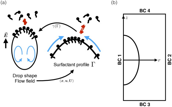
Figure 12: (a) The numerical algorithm for the second-order immersed interface method code: At $t_{n}$ the drop shape $\bm{x}$, flow field $\bm{u}$, and interface velocity, $\bm{U}$ are computed using the electrohydrodynamic solver in Nganguia et al. (2015, 2016). The information is then used as input to the surfactant transport solver Hu et al. (2018), in order to determine the bulk ($\phi$) and interface surfactant profile ($\Gamma$). Given $\Gamma$, we determine the change in surface tension $\gamma$, as well as the updated drop shape, flow field, and interface velocity at time $t_{n+1}$. This process is repeated either until a steady-state is reached, or up to the onset of drop break-up. Flow circulation and direction are represented by the blue arrows. (b) Computational domain on the $(r,z)$-plane. On the walls BC 1, 2, 3, and 4 denote the boundary conditions (see text)

Figure 12a illustrates the algorithm. The droplet shape and position $\bm{x}$, flow field $\bm{u}$ and interface velocity $\bm{U}$ are computed using the IIM solver in Nganguia et al. (2015, 2016). The boundary conditions in the computational domain $\Omega=[0,L]\times[-L,L]$ in figure 12b are given as follows: for the electric potential, $\phi^{+}=\mp E_{0}L/2$ at $z=\pm L$ (the bottom BC3 and top BC4 of the computational domain), while a Neumann boundary condition $\partial\phi/\partial r=0$ is imposed on the sides ($r=0,\;L$) of the computational domain. For the Stokes equations, the pressure and velocity $\partial p/\partial r=0$, $\partial w/\partial r=0$, $u=0$ at $r=0$ (BC1), while Dirichlet boundary conditions are imposed on the other three sides (BC2-BC4) Nganguia et al. (2015). For the bulk surfactant concentration $C$, Neumann (BC1) and no flux (zero Neumann) (BC2-BC4) boundary conditions are imposed Hu et al. (2018).

For more detailed implementation steps and numerical methods, the reader is referred to Nganguia et al. (2015) for the electrohydrodynamic solver. The three-dimensional axisymmetric soluble surfactant solver is a straightforward extension of the two-dimensional scheme in Hu et al. (2018). The main difference is in the treatment of the correction term for the curvature at the irregular grid nodes.

Appendix B Validation

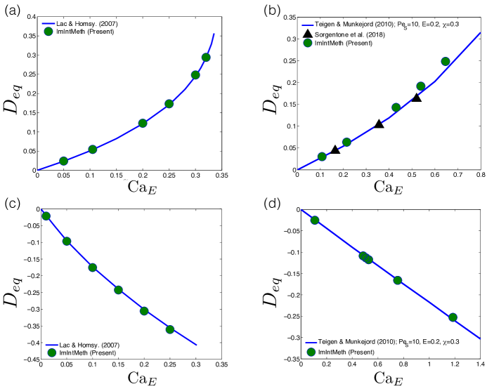
Figure 13: Comparison between published simulation results for the clean drop case (a&c) in Lac and Homsy (2007) and the surfactant-covered drop cases (b&d) in Teigen and Munkejord (2010); Sorgentone et al. (2019). The solid lines represent simulations from boundary integral for the clean case, and from level-set for the surfactant-covered drop case. The black triangles represent simulations from boundary integral, while the green circles represent simulations using the proposed immersed interface (IIM) implementation. For the clean drop cases: (a) $\sigma_{r}=0.1,\;\varepsilon_{r}=0.1$; (c) $\sigma_{r}=0.5,\;\varepsilon_{r}=20$. For the surfactant-covered drop cases we set $E=0.2,\;\chi=0.3,\;\text{Pe}_{s}=10,\;\text{Bi}=0$: (b) $\sigma_{r}=0.3,\;\varepsilon_{r}=1$; (d) $\sigma_{r}=1,\;\varepsilon_{r}=2$. Volume and total surfactant are conserved to within 5% in all cases.

We validate our numerical codes by comparing against results in the literature where the equilibrium deformation number (Eq. 18) is reported as a function of the electric capillary number $\text{Ca}_{E}$, for both a clean drop and and a drop laden with insoluble surfactant. $L$ and $B$ are the drop size along the major and minor axes, respectively. At moderate $\text{Ca}_{E}$, the equilibrium drop shape under a DC electric field could be either prolate or oblate. For an oblate drop, the circulation is always from the pole to the equator, while the flow inside a prolate drop can be ieither from the equator to the pole (prolate ‘A’) or from the pole to the equator (prolate ‘B’). In our simulations the computational domain size is $[0,5]\times[-5,5]$. The step size $h=5/N$ where $N=256$, and the time step $\Delta t=h/10$.

Figure 13 shows comparisons for a clean drop (a&c) and for a surfactant-covered drop (b&d). We test our implementation against the boundary integral (BI) results from figures 5, and 19 in Lac and Homsy (2007). Figure 13a shows the equilibrium deformation number $D_{eq}$ as a function of the capillary number $\text{Ca}_{E}$ for a prolate drop with $\sigma_{r}=0.1,\;\varepsilon_{r}=0.1$, while the oblate drop is shown in figure 13c with $\sigma_{r}=0.5,\;\varepsilon_{r}=20$. These comparisons show good agreement with the present immersed interface method (IIM) results.

For the surfactant-covered drop, we consider the work in Teigen and Munkejord (2010); Sorgentone et al. (2019) to validate the prolate and the oblate shapes. For these simulations, the electric parameters are set to $\sigma_{r}=0.3,\;\varepsilon_{r}=1$ for the prolate drop (case A in Teigen and Munkejord (2010)), and $\sigma_{r}=1,\;\varepsilon_{r}=2$ for the oblate drop (case C in Teigen and Munkejord (2010)). The elasticity constant $E=0.2$ and the surfactant coverage $\chi=0.3$. Other surfactant-related parameters are as follows: the surface and bulk Peclet numbers $\text{Pe}_{S}=\text{Pe}=10$, respectively, and the Biot number $\text{Bi}=0$ (the insoluble surfactant limit). Figures 13b and 13d show excellent agreement between all three numerical methods: boundary integral (BI), immersed interface method (IIM), and regularized level-set method (RLSM).

Appendix C Mesh refinement study

We perform a grid analysis (or mesh refinement) study. We consider a computational domain $\Omega=[0,5]\times[-5,5]$, to compute the $L_{\infty}$ error and determine the ratio

$$\text{Rate = }\dfrac{||A_{N}-A_{2N}||_{\infty}}{||A_{2N}-A_{4N}||_{\infty}},$$ (20)

where $N$ is the grid size. The number of Lagrangian markers for the interface $M=N/2$. We run simulations to a final time $T=0.5$ with time step $\Delta t=10^{-3}$. The electric parameters are $\text{Ca}_{E}=0.1$, $\varepsilon_{r}=1$, $\sigma_{r}=0.3$, corresponding to the prolate ‘A’ drop shape (case A in Teigen and Munkejord (2010)). The surfactant parameters are $E=0.2$, $\text{Pe}=10$, $\text{Pe}_{s}=10$, $\chi=0.3$, and the solubility parameter $\text{Bi}=0.01$. Tables 3-5 show the results of the analysis.

Table 3: Numerical convergence for the flow field variables $\bm{u}=(u,v)$ and the pressure $p$.

$N$	$||u_{N}-u_{2N}||_{\infty}$	rate	$||w_{N}-w_{2N}||_{\infty}$	rate	$||p_{N}-p_{2N}||_{\infty}$	rate
32	$1.769\times 10^{-1}$	$-$	$1.777\times 10^{-1}$	$-$	$7.303$	$-$
64	$2.724\times 10^{-2}$	$2.7$	$1.086\times 10^{-1}$	$0.711$	$5.408\times 10^{-2}$	$7.08$
128	$2.436\times 10^{-2}$	$0.161$	$4.21\times 10^{-2}$	$1.37$	$1.402\times 10^{-2}$	$1.95$
256	$2.498\times 10^{-3}$	$3.29$	$9.36\times 10^{-3}$	$2.17$	$2.025\times 10^{-3}$	$2.79$

Table 4: Numerical convergence for the component of interface markers $\bm{X}=(X,Y)$, the surface surfactant concentration $\Gamma$, the surface tension $\gamma$ and surface tension gradient ${\rm~{}d}\gamma$.

$M$	$||\bm{X}_{M}-\bm{X}_{2M}||_{\infty}$	rate	$||\Gamma_{M}-\Gamma_{2M}||_{\infty}$	rate
16	$4.384\times 10^{-2}$	$-$	$1.053\times 10^{-1}$	$-$
32	$2.29\times 10^{-3}$	$4.29$	$9.954\times 10^{-3}$	$3.4$
64	$4.992\times 10^{-4}$	$2.17$	$1.72\times 10^{-3}$	$2.53$
128	$1.07\times 10^{-4}$	$2.2$	$5.522\times 10^{-4}$	$1.64$
$M$	$||\gamma_{M}-\gamma_{2M}||_{\infty}$	rate	$||{\rm~{}d}\gamma_{M}-{\rm~{}d}\gamma_{2M}||_{\infty}$	rate
16	$9.213\times 10^{-3}$	$-$	$2.27\times 10^{-3}$	$-$
32	$8.493\times 10^{-4}$	$3.44$	$1.223\times 10^{-3}$	$0.892$
64	$1.477\times 10^{-4}$	$2.52$	$2.897\times 10^{-4}$	$2.08$
128	$4.744\times 10^{-5}$	$1.64$	$4.765\times 10^{-5}$	$2.6$

Table 5: Numerical convergence for the staggered variables: the electric potential ($\phi$) and the bulk surfactant concentration ($C$).

$N$	$||\phi_{N}-\phi_{2N}||_{\infty}$	rate	$||C_{N}-C_{2N}||_{\infty}$	rate
32	$1.556$	$-$	$2.016$	$-$
64	$4.179\times 10^{-1}$	$1.9$	$1.691$	$0.254$
128	$6.779\times 10^{-2}$	$2.62$	$1.451$	$0.221$
256	$1.035\times 10^{-2}$	$2.71$	$6.025\times 10^{-1}$	$1.27$

Appendix D Flow fields at high values of the transfer parameter

References

- Saville (1970) D. A. Saville, “Electrohydrodynamic stability: Fluid cylinders in longitudinal electric fields,” Phys. Fluids 13, 2987–2994 (1970).
- Ramos et al. (1998) A. Ramos, H. Morgan, N. G. Green, and A. Castellanos, “Ac electrokinetics: a review of forces in microelectrode structures,” J. Phys. D: Appl. Phys. 31, 2338 (1998).
- Ramos et al. (1999) A. Ramos, H. Morgan, N. G. Green, and A. Castellanos, “Ac electric-field-induced fluid flow in microelectrodes,” J. Colloid Interface Sci. 217, 420–422 (1999).
- Castellanos et al. (2003) A. Castellanos, A. Ramos, A. Gonzalez, N. G. Green, and H. Morgan, “Electrohydrodynamics and dielectrophoresis in microsystems: scaling laws,” J. Phys. D: Appl. Phys. 36, 2584–2597 (2003).
- Bazant and Squires (2004) M. Z. Bazant and T. M. Squires, “Induced-charge electrokinetic phenomena: Theory and microfluidic applications,” Phys. Rev. Lett. 92, 066101 (2004).
- Velev and Bhatt (2006) O. D. Velev and K. H. Bhatt, “On-chip micromanipulation and assembly of colloidal particles by electric fields,” Soft Matter 2, 738 (2006).
- Hayati et al. (1986) I. Hayati, A. I. Bailey, and T. F. Tadros, “Mechanism of stable jet formation in electrohydrodynamic atomization,” Nature 319, 41–43 (1986).
- Ramos and Castellanos (1994) A. Ramos and A. Castellanos, “Conical points in liquid-liquid interfaces subjected to electric fields,” Phys. Lett. A 184, 268–272 (1994).
- Ramos et al. (1994) A. Ramos, H. Gonzalez, and A. Castellanos, “Experiments on dielectric liquid bridges subjected to axial electric fields,” Phys. Fluids 6, 3206–3208 (1994).
- Saville (1993) D. A. Saville, “Electrohydrodynamic deformation of a particulate stream by a transverse electric field,” Phys. Rev. Lett. 71, 2907–2910 (1993).
- Torza et al. (1971) S. Torza, R. G. Cox, and S. G. Mason, “Electrohydrodynmaic deformation and burst of liquid drops,” Proc. R. Soc. Lond. A 269, 295–319 (1971).
- Sherwood (1988) J. D. Sherwood, “Breakup of fluid droplets in electric and magnetic fields,” J. Fluid Mech. 188, 133–146 (1988).
- Trau et al. (1996) M. Trau, D. A. Saville, and I. A. Aksay, “Field-induced layering of colloidal crystals,” Science 272, 706–709 (1996).
- Trau et al. (1997) M. Trau, D. A. Saville, and I. A. Aksay, “Assembly of colloidal crystals at electrode interfaces,” Langmuir 13, 6375–6381 (1997).
- Vaidyanathan et al. (2015) R. Vaidyanathan, S. Dey, L. G. Carrascosa, M. J. A. Shiddiky, and M. Trau, “Alternating current electrohydrodynamics in microsystems: Pushing biomolecules and cells around on surfaces,” Biomicrofluidics 9, 061501 (2015).
- Mori and Young (2018) Y. Mori and Y.-N. Young, “From electrodiffusion theory to the electrohydrodynamics of leaky dielectrics through the weak electrolyte limit,” J. Fluid Mech. 855, 67–130 (2018).
- O’Konski and Thacher (1953) C. T. O’Konski and H. C. Thacher, “The distortion of aerosol droplets by an electric field,” J. Chem. Phys. 57, 955–958 (1953).
- Allan and Mason (1962) R. S. Allan and S. G. Mason, “Particle behaviour in shear and electric fields. I. Deformation and burst of fluid drops,” Proc. R. Soc. Lond. A 267, 45–61 (1962).
- Taylor (1966) Geoffrey Taylor, “Studies in electrohydrodynamics. I. the circulation produced in a drop by electric field,” Proc. R. Soc. Lond. A 291, 159–166 (1966).
- Melcher and Taylor (1969) J. R. Melcher and G. I. Taylor, “Electrohydrodynamics: A review of the role of interfacial shear stresses,” Annu. Rev. Fluid Mech. 1, 111–146 (1969).
- Lanauze et al. (2013) J. A. Lanauze, L. M. Walker, and A. S. Khair, “The influence of inertia and charge relaxation on electrohydrodynamic drop deformation,” Phys. Fluids 25, 112101 (2013).
- Lanauze et al. (2015) J. A. Lanauze, L. M. Walker, and A. S. Khair, “Nonlinear electrohydrodynamics of slightly deformed oblate drops,” J. Fluid Mech. 774, 245 (2015).
- Mandal et al. (2016a) S. Mandal, A. Bandopadhyay, and S. Chakraborty, “Effect of surface charge convection and shape deformation on the dielectrophoretic motion of a liquid drop,” Phys. Rev. E 93, 043127 (2016a).
- Mandal et al. (2017) S. Mandal, A. Bandopadhyay, and S. Chakraborty, “The effect of surface charge convection and shape deformation on the settling velocity of drops in nonuniform electric field,” Phys. Fluids 29, 012101 (2017).
- Das and Saintillan (2017a) D. Das and D. Saintillan, “A nonlinear small-deformation theory for transient droplet electrohydrodynamics,” J. Fluid Mech. 810, 225 (2017a).
- Bentenitis and Krause (2005) N. Bentenitis and S. Krause, “Droplet deformation in DC electric fields: The extended leaky dielectric model,” Langmuir 21, 6194–6209 (2005).
- Zhang et al. (2013) J. Zhang, J. D. Zahn, and H. Lin, “Transient solution for droplet deformation under electric fields,” Phys. Rev. E 87, 043008 (2013).
- Zabarankin (2013) M. Zabarankin, “A liquid spheroidal drop in a viscous incompressible fluid under a steady electric field,” SIAM J. Appl. Math. 73, 677–699 (2013).
- Zabarankin (2016) M. Zabarankin, “Analytical solution for spheroidal drop under axisymmetric linearized boundary conditions,” SIAM J. Appl. Math. 76, 1606–1632 (2016).
- Brazier-Smith (1971) P. R. Brazier-Smith, “Stability and shape of isolated and pairs of water drops in an electric field,” Phys. Fluids 14, 1 (1971).
- Brazier-Smith et al. (1971) P. R. Brazier-Smith, S. G. Jennings, and J. Latham, “An investigation of the behaviour of drops and drop-pairs subjected to strong electric forces,” Proc. R. Soc. Lond. A 325, 363–376 (1971).
- Miksis (1981) M. Miksis, “Shape of a drop in an electric field,” Phys. Fluids 24, 1967 (1981).
- Basaran and Scriven (1989) O. A. Basaran and L. E. Scriven, “Axisymmetric shapes and stability of charged drops in an external electric field,” Phys. Fluids 1, 799 (1989).
- Supeene et al. (2008) G. Supeene, C. R. Koch, and S. Bhattacharjee, “Deformation of a droplet in an electric field: Nonlinear transient response in perfect and leaky dielectric mdeia,” J. Colloid Int. Sci. 318, 463–376 (2008).
- Nganguia et al. (2015) H. Nganguia, Y.-N. Young, A. T. Layton, W.-F. Hu, and M.-C. Lai, “An immersed interface method for axisymmetric electrohydrodynamic simulations in stokes flow,” Commun. Comput. Phys. 18, 429–449 (2015).
- Hu et al. (2014) W.-F. Hu, M.-C. Lai, and Y.-N. Young, “A hybrid immersed boundary and immersed interface method for electrohydrodynamic simulations,” J. Comp. Phys. 282, 47–61 (2014).
- Saville (1997) D. A. Saville, “Electrohydrodynamics: The Taylor-Melcher leaky dielectric model,” Annu. Rev. Fluid Mech. 29, 27–64 (1997).
- Ha and Yang (2000a) J.-W. Ha and S.-M. Yang, “Deformation and breakup of Newtonian and non-Newtonian conducting drops in an electric field,” J. Fluid Mech. 405, 131–156 (2000a).
- Zholkovskij et al. (2002) E. K. Zholkovskij, J. H. Masliyah, and J. Czarnecki, “An electrokinetic model of drop deformation in an electric field,” J. Fluid Mech. 472, 1–27 (2002).
- Ha and Yang (2000b) J.-W. Ha and S.-M. Yang, “Electrohydrodynamics and electrorotation of a drop with fluid less conducting than that of the ambient fluid,” Phys. Fluids 12, 764 (2000b).
- Lac and Homsy (2007) E. Lac and G. M. Homsy, “Axisymmetric deformation and stability of a viscous drop in a steady electric field,” J. Fluid Mech. 590, 239 (2007).
- Ha and Yang (1995) J.-W. Ha and S.-M. Yang, “Effects of surfactant on the deformation and stability of a drop in a viscous fluid in an electric field,” J. Colloid Int. Sci. 175, 369–385 (1995).
- Teigen and Munkejord (2010) K. E. Teigen and S. T. Munkejord, “Influence of surfactant on drop deformation in an electric field,” Phys. Fluids 22, 112104 (2010).
- Nganguia et al. (2013) H. Nganguia, Y.-N. Young, P. M. Vlahovska, J. Bławzdziewcz, J. Zhang, and H. Lin, “Equilibrium electro-deformation of a surfactant-laden viscous drop,” Phys. Fluids 25, 092106 (2013).
- Nganguia et al. (2019) H. Nganguia, O. S. Pak, and Y.-N. Young, “Effects of surfactant transport on electrodeformation of a viscous drop,” Phys. Rev. E 99, 063104 (2019).
- Lanauze et al. (2018) J. A. Lanauze, R. Sengupta, B. J. Bleier, B. A. Yezer, A. S. Khair, and L. M. Walker, “Colloidal stability dictates drop breakup under electric fields,” Soft Matter 14, 9351–9360 (2018).
- Sorgentone et al. (2019) C. Sorgentone, A.-K. Tornberg, and P. Vlahovska, “A 3D boundary integral method for the electrohydrodynamics of surfactant-covered drops,” J. Comput. Phys. 389, 111–127 (2019).
- Poddar et al. (2018) A. Poddar, S. Mandal, A. Bandopadhyay, and S. Chakraborty, “Sedimentation of a surfactant-laden drop under the influence of an electric field,” J. Fluid Mech. 849, 277–311 (2018).
- Poddar et al. (2019a) A. Poddar, S. Mandal, A. Bandopadhyay, and S. Chakraborty, “Electrical switching of a surfactant coated drop in poiseuille flow,” J. Fluid Mech. 870, 27–66 (2019a).
- Poddar et al. (2019b) A. Poddar, S. Mandal, A. Bandopadhyay, and S. Chakraborty, “Electrorheology of a dilute emulsion of surfactant-covered drops,” J. Fluid Mech. 881, 524–550 (2019b).
- Mandal et al. (2016b) S. Mandal, A. Bandopadhyay, and S. Chakraborty, “Dielectrophoresis of a surfactant-laden viscous drop,” Phys. Fluids 28, 062006 (2016b).
- Ouriemi and Vlahovska (2014) M. Ouriemi and P. M. Vlahovska, “Electrohydrodynamics of particle-covered drops,” J. Fluid Mech. 751, 106–120 (2014).
- Zhang et al. (2015) L. Zhang, L. He, M. Ghadiri, and A. Hassanpour, “Effect of surfactants on the deformation and break-up of an aqueous drop in oils under high electric field strengths,” J. Pet. Sci. Eng. 125, 38–47 (2015).
- Luo et al. (2018) X. Luo, X. Huang, H. Yan, D. Yang, J. Wang, and L. He, “Breakup modes and criterion of droplet with surfactant under direct current electric field,” Chem. Eng. Res. Des. 132, 822–830 (2018).
- Sengupta et al. (2019) R. Sengupta, A. S. Khair, and L. M. Walker, “Electric fields enable tunable surfactant transport to micro scale fluid interfaces,” Phys. Rev. E 100, 023114 (2019).
- Chen and Stebe (1996) J. Chen and K. Stebe, “Marangoni retardation of the terminal velocity of a settling droplet: Role of surfactant physico-chemistry,” J. Colloid Interface Sci. 178, 144–155 (1996).
- Eggleton and Stebe (1998) C. D. Eggleton and K. J. Stebe, “An adsoprtion-desorption-controlled surfactant on a deforming droplet,” J. Coll. Int. Sci. 208, 68 (1998).
- Blawzdziewicz et al. (1999) J. Blawzdziewicz, E. Wajnryb, and M. Loewenberg, “Hydrodynamic interactions and collision efficiencies of spherical drops covered with an incompressible surfactant film,” J. Fluid Mech. 395, 29–59 (1999).
- Zholkovskij et al. (2000) E. K. Zholkovskij, V. I. Kovalchuk, S. S. Dukhin, and R. Miller, “Dynamics of rear stagnant cap formation at low reynolds numbers 1. slow sorption kinetics,” J. Colloid Interface Sci. 226, 51–59 (2000).
- Milliken and Leal (1994) W. J. Milliken and L. G. Leal, “The influence of surfactant on the deformation and breakup of a viscous drop: the effect of surfactant solubility,” J. Coll. Int. Sci. 166, 275–285 (1994).
- Hanyak et al. (2012) M. Hanyak, D. K. N. Sinz, and A. A. Darhuber, “Soluble surfactant spreading on spatially confined thin liquid films,” Soft Matt. 8, 7660 (2012).
- Roux et al. (2016) S. Le Roux, M. Roche, I. Cantat, and A. Saint-Jalmes, “Soluble surfactant spreading: How the amphiphilicity sets the marangoni hydrodynamics,” Phys. Rev. E 93, 013107 (2016).
- Sellier and Panda (2017) M. Sellier and S. Panda, “Unraveling surfactant transport on a thin liquid film,” Wave Motion 70, 183–194 (2017).
- Thiele et al. (2016) U. Thiele, A. J. Archer, and L. M. Pismen, “Gradient dynamics models for liquid films with soluble surfactant,” Phys. Rev. Fluids 1, 083903 (2016).
- Li and Gupta (2019) W. Li and N. R. Gupta, “Buoyancy-driven motion of bubbles in the presence of soluble surfactants in a newtonian fluid,” Ind. Eng. Chem. Res. 58, 7640–7649 (2019).
- Das and Saintillan (2017b) D. Das and D. Saintillan, “Electrohydrodynamics of viscous drops in strong electric fields: numerical simulations,” J. Fluid Mech. 829, 127 (2017b).
- Chang and Franses (1995) C.-H. Chang and E. I. Franses, “Adsorption dynamics of surfactants at the air/water interface: a critical review of mathematical models, data and mechanisms,” Colloids and Surfaces 100, 1–45 (1995).
- Wang et al. (2014) Q. Wang, M. Siegel, and M. R. Booty, “Numerical simulation of drop and bubble dynamics with soluble surfactant,” Phys. Fluids 26, 052102 (2014).
- Pawar and Stebe (1996) Y. Pawar and K. J. Stebe, “Marangoni effects on drop deformation in an extensional flow: The role of surfactant physical chemistry. I Insoluble surfactants,” Phys. Fluids 8 (7), 1738–1751 (1996).
- Weidner (2013) D. E. Weidner, “Suppression and reversal of drop formation on horizontal cylinders due to surfactant convection,” Phys. Fluids 25, 082110 (2013).
- Kallendorf et al. (2015) C. Kallendorf, A. Fath, M. Oberlack, and Y. Wang, “Exact solutions to the interfacial surfactant transport equation on a droplet in a Stokes flow regime,” Phys. Fluids 27, 082104 (2015).
- Muradoglu and Tryggvason (2008) M. Muradoglu and G. Tryggvason, “A front-tracking method for computation of interfacial flows with soluble surfactants,” J. Comp. Phys. 227, 2238–2262 (2008).
- Lai et al. (2011) M.-C. Lai, C.-Y. Huang, and Y.-M. Huang, “Simulating the axisymmetric interfacial flows with insoluble surfactant by immersed boundary method,” Int. J. Numer. Anal. Mod. 8, 105–117 (2011).
- Xu et al. (2014) J.-J. Xu, Y. Huang, M.-C. Lai, and Z. Li, “A coupled immersed interface and level set method for three-dimensional interfacial flows with insoluble surfactant,” Commun. Comput. Phys. 15, 451–469 (2014).
- Xu et al. (2018) J.-J. Xu, W. Shi, and M.-C. Lai, “A level set method for two-phase flows with soluble surfactant,” J. Comput. Phys. 353, 336–355 (2018).
- Sorgentone and Tornberg (2018) C. Sorgentone and A.-K. Tornberg, “A highly accurate boundary integral equation method for surfactant-laden drops in 3D,” J. Comput. Physics 360, 167–191 (2018).
- Nganguia et al. (2016) H. Nganguia, Y.-N. Young, A. T. Layton, M.-C. Lai, and W.-F. Hu, “Electrohydrodynamics of a viscous drop with inertia,” Phys. Rev. E 93, 053114 (2016).
- Hu et al. (2018) W.-F. Hu, M.-C. Lai, and C. Misbah, “A coupled immersed boundary and immersed interface method for interfacial flows with soluble surfactant,” Comput. Fluids 168, 201–215 (2018).
- Ha and Yang (1998) J.-W. Ha and S.-M. Yang, “Effect of nonionic surfactant on the deformation and breakup of a drop in an electric field,” J. Colloid Int. Sci. 206, 195–204 (1998).
- Anna and Mayer (2006) S. L. Anna and H. C. Mayer, “Microscale tipstreaming in a microfluidic flow focusing device,” Phys. Fluids 18, 121512 (2006).
- Alvarez et al. (2010) N. J. Alvarez, L. M. Walker, and S. L. Anna, “A microtensiometer to probe the effect of radius of curvature on surfactant transport to a spherical interface,” Langmuir 26, 13310–13319 (2010).
- Alvarez et al. (2011) N. J. Alvarez, W. Lee, L. M. Walker, and S. L. Anna, “The effect of alkane tail length of CiE8 surfactants on transport to the silicone oil-water interface,” J. Colloid Interface Sci. 355, 231–236 (2011).
- Alvarez et al. (2012) N. J. Alvarez, D. R. Vogus, L. M. Walker, and S. L. Anna, “Using bulk convection in a microtensiometer to approach kinetic-limited surfactant dynamics at fluid-fluid interfaces,” J. Colloid Interface Sci. 372, 183–191 (2012).