Levitating Rigid Objects with Hidden Rods and Wires

Abstract

We propose a novel algorithm to efficiently generate hidden structures to support arrangements of floating rigid objects. Our optimization finds a small set of rods and wires between objects and each other or a supporting surface (e.g., wall or ceiling) that hold all objects in force and torque equilibrium. Our objective function includes a sparsity inducing total volume term and a linear visibility term based on efficiently pre-computed Monte-Carlo integration, to encourage solutions that are as-hidden-as-possible. The resulting optimization is convex and the global optimum can be efficiently recovered via a linear program. Our representation allows for a user-controllable mixture of tension-, compression-, and shear-resistant rods or tension-only wires. We explore applications to theatre set design, museum exhibit curation, and other artistic endeavours.

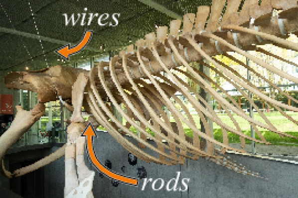
Figure 1: The skeleton of a blue whale levitates with the support of wires from above and internal rods.

1 Introduction

Levitating objects are visually compelling and commonly found in artistic sculptures, film and theatre set design, promotional displays, and museum exhibits (see Figure 1 and Figure 3). This effect is especially impressive if the support structure can be hidden from the observer, removing its unsightly distraction and perhaps even giving the impression that the objects in the arrangement are magically floating in space (see Figure Levitating Rigid Objects with Hidden Rods and Wires). Achieving this is a non-trivial task. Physical stability requires a balance of force and torque for each rigid component of the scene. This is readily achieved using many strong, thick struts, but their geometry and scene placement is likely to compete for visual attention with scene objects, or worse, visually obscure objects in the scene (see Figure 2). Hiding these supports by removing or thinning too many struts, on the other hand, will sacrifice physical stability. Thin wires can sometimes be used to hang objects, but wires only resist tension so they alone can not handle situations that are not supported purely from above.

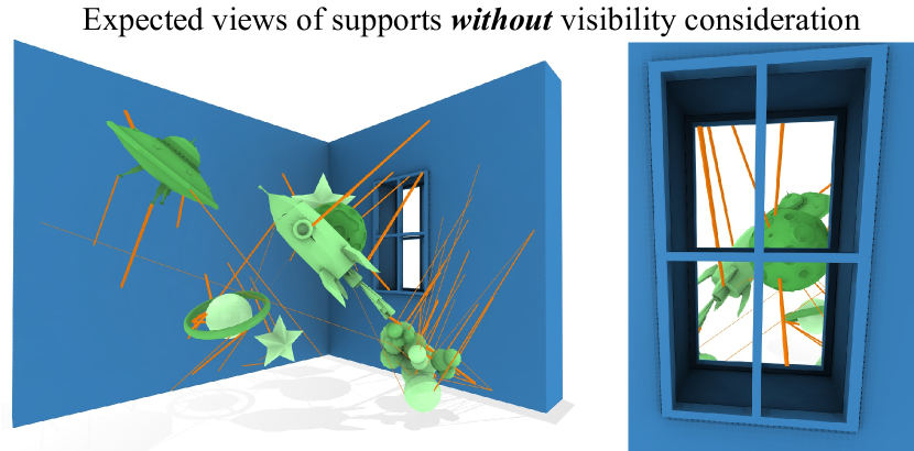
Figure 2: Without our visibility term, optimal rods may be an unsightly distraction.

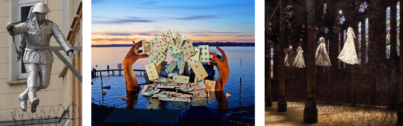
Figure 3: Levitating objects have inspired such artworks as a sculpture of border guard Conrad Schumann jumping (left), an enormous stage display of playing cards by Es Devlin for the Bregenz Festival (middle), and Chiharu Shiota’s installation where white dresses float overhead (right).

In this paper, we propose modeling the problem of hidden support structure generation for levitating objects as a form of topology optimization. We present a novel convex optimization based on the well-established ground structure method from architecture and engineering. The input to our method is an arrangement of objects in their desired locations and orientations and the distribution of views from which the scene will likely be observed. Our output is a collection of rods and wires, described by their required thicknesses and attachment points on the input rigid objects, and the supporting structural element (e.g., wall or ceiling). Our rods model tension, compression and bending resistant materials (e.g., wooden dowel rods or steel beams). Our wires model tension only (e.g., fishing line or steel cables).

Unlike Computer Graphics or Virtual Reality where physical laws can be bent or broken, support structures in real scenes are only meaningful if physically valid. Therefore, we enforce physical validity in our optimization as a hard constraint: namely that the rigid objects should achieve force and torque equilibrium and that stresses on rods and wires do not exceed material-dependent yield limits. For ease of assembly, cost of manufacturing, and visibility considerations, we prefer support structures composed of a small number of thin, less visible supports. We model these criteria with a sparsity-inducing cost function defined as a sum over a densely connected graph of edges (i.e., the ground structure).

Treating the cross-sectional area of each edge as the primary optimization variable, the traditional ground structure method optimizes the total volume (linear in the areas since lengths are predetermined) and enforces force balance at point loads, by measuring linearized axial tension and compression forces from each rod, subject to yield limits, expressed as linear inequalities in the unknown cross-section areas and axial stresses of the rods. The result is a linear program whose solution — like many $L_{1}$ or Lasso problems — is sparse (most areas are exactly zero), and often agrees exactly with the NP-hard selection problem (picking the smallest valid subset of edges).

We augment the traditional ground structure method to support embedded rigid objects (via linear static equilibrium equations) and account for bending resistance of rods (via a simple linear shearing model derived from proportionality assumptions). We introduce a visibility objective function that is also linear in the unknown edge areas and relies on efficient Monte-Carlo based precomputation. Thus, the optimization remains a (convex) linear program and solutions can be extracted efficiently (in usually less than a minute).

Our experiments satisfyingly confirm that under many conditions structurally valid supports are lurking just out of sight: the space of physically valid supports is vast and finding a completely occluded arrangement is often possible. We demonstrate the effectiveness of our method across a wide variety of test scenes and prototypical use cases.

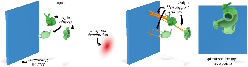
Figure 4: The input to our method is a scene composed of many levitating rigid objects. The output of our method is a collection of rods tucked away behind object occlusions, holding each object in force and torque equilibrium under gravity.

2 Related Work

Our work sits within the larger literature of computational fabrication, construction and assembly. These subfields are rich and vast, so we focus on previous works most similar in methodology or application.

Previous algorithms exist to make objects stand [PWLS13, VHWP12], spin [BWBS14] or hang from wires [MML16]. These works modify the input objects by redistributing mass or changing their shape to achieve the desired goal. In this paper, we explore a complementary contract with the user — how to anchor objects in the environment without changing the objects themselves. We do not assume that objects were fabricated in a particular manner (e.g., 3D printing).

Our approach may be categorized with other structural optimizations for a prescribed static load scenario (i.e., ignoring inertial forces). Recent works increase the stability of fragile objects by adding new structural elements [ZPZ13, SVB*12, CZT16]. For example, Stava et al. add struts to 3D printed objects one-by-one as part of a large optimization loop and use a volumetric simulation as validation. Their strut selection includes an ambient occlusion visibility term, but they do not consider the problem of selecting an optimal set of supports for rigid objects under prescribed viewing conditions. Other methods have considered the interactive design of rod-structures  [PTC*15, KSW*17, CZS*19, Jac19] with varying degrees of physical feasibility checking or optimization in the system.

We model the problem of hiding support structures as a form of topology optimization [LGC*18]. The general idea of topology optimization is to prune away material from the volume around the input objects or load conditions. The resulting geometries typically have interesting topologies/connectivities that would have been difficult to determine a priori. Methods that determine the material occupancy of each voxel in a dense grid are well suited for 3D printing and milling (e.g., [WDW16]), but will in general produce geometries composed curved and varying thickness elements. Our method instead belongs to the class of ground structure methods [Dor64], which output a discrete collection of (straight) elements from an initial over-connected graph of candidates (see Figure 8). Methodologically we follow most closely the stress-based formulation of Zegard et al. [ZP15], and utilize the thesis of Freund [Fre04] as a reference. Ground structure-like methods have been applied for designing everything from buildings [ZHMB20] and glass shell structures  [FLM*20] to construction supports [DPW*14] to 3D printable models [WWY*13, JTSW17, HZH*16] to cable-driven automata [MKS*17]. The standard ground structure method considers only axial forces. These methods have been applied for rigid structural elements and adapted to special cases like tensegrities [PTV*17, CW96].

We use a ground structure approach to model the novel problem of creating hidden structural supports from complex viewpoint distributions. Crucially, our method supports structural elements that resist compression, tension and bending forces, as well as wires, without resorting to the nonlinear constitutive models or volumetric meshing of prior work [SVB*12, PTC*15, HZH*16]. Our method trivially couples the structure to the rigid objects it supports, correctly accounting for both linear forces and torques, without resorting to displacement-based mechanical formulations (e.g., [PTV*17]). This allows us to formulate our problem as a linear program which can be solved efficiently.

We draw inspiration from algorithms for appearance-driven optimization. For instance, Schuller et al. introduce the problem of generating appearance mimicking surfaces from a specified viewpoint [SPS14]. Several works seek to create 3D shapes that take the form of a set of 2D shapes from corresponding viewpoints or cast the 2D image under certain lighting conditions [MP09, HHC18, STTP14]. Others use viewpoints to create optimal perceptual experiences, for example in 3D printing support structures [ZLP*15] or in skyscraper design [DFL*15].

3 Method

The input to our method is a scene comprised of $K$ rigid objects oriented and positioned in space, a fixed support surface (e.g., wall or ceiling), and a distribution of viewpoints (e.g., discrete set of positions or sample-able probability density function defined on a surface) The output of our method is a supporting structure composed of a small set of rods and wires connecting rigid objects to each other or the supporting surface. Our method ensures that this structure holds the input objects in their prescribed positions and orientations, counter-balancing the force these objects experience due to gravity. Our method optimizes the size and placement of the structure to minimize its overall volume and its visibility with respect to the input viewpoint distribution (see Figure 4). Before describing our optimization, we define our physical model and how we measure visibility.

3.1 Rigid Body Equilibrium

The rigid objects in our scenes experience forces from gravity and at the points of attachment to the supporting structure. To hold a rigid body at rest, we must maintain force and torque equilibrium:

$$\sum\limits_{i\in V_{k}}\mathbf{f}_{i} =m_{k}\mathbf{g},$$ (1)

$$\sum\limits_{i\in V_{k}}\underbrace{(\mathbf{x}_{i}-\overline{\mathbf{x}}_{k})\times\mathbf{f}_{i}}_{\boldsymbol{\tau}_{i}} =\mathbf{0},$$ (2)

where $m_{k}$, $\overline{\mathbf{x}}_{k}$, and $V_{k}$ are the mass, center of mass, and set of attachment points of the $k$th object, respectively, and $\mathbf{x}_{i},\mathbf{f}_{i},\boldsymbol{\tau}_{i}$ are the 3D position of the $i$th attachment point and corresponding force and torque vectors, respectively.

3.2 Rods

We assume our support structure undergoes negligible displacement, affording a linearization of the internal forces at play. For stiff rods, we follow the linearized tension and compression model of [ZP15, Fre04], which introduces a signed scalar value per rod $c_{ij}\in\mathbb{R}$ with units Newtons describing the force in the axial direction parallel to the rod. Assigning an arbitrary direction to the rod $ij$ between endpoint positions $\mathbf{x}_{i}$ and $\mathbf{x}_{j}$, then the axial force contribution at endpoints $i$ and $j$ are the product of this scalar $c_{ij}$ by the rod’s tangent unit direction $\hat{\mathbf{t}}_{ij}=(\mathbf{x}_{i}-\mathbf{x}_{j})/\|\mathbf{x}_{i}-\mathbf{x}_{j}\|$:

$$\mathbf{f}_{i}\mathrel{+}=c_{ij}\hat{\mathbf{t}}_{ij}\quad\text{ and }\quad\mathbf{f}_{j}\mathrel{-}=c_{ij}\hat{\mathbf{t}}_{ij}.$$ (3)

Previous methods (e.g., [ZP15, Fre04]) rely solely on tension and compression and ignoring the rods’ resistance to bending. This is a reasonable assumption in architecture where loads are large relative to the rod’s bending strength. Ignoring bending requires that the rods are thicker and thus more visible (see Figure 6). This is at odds with the intuition that light loads can be held up with a single bending-resistant rod. In reality, a single rod with finite thickness can apply a distribution of forces over its non-zero area contact surface. Since the force is applied at more than one point, torque balance is also possible. Unfortunately, a volumetric rod model couples the unknown rod diameters and forces non-linearly.

To maintain the linearity of our system but also account for bending, we introduce a linearized shearing model to account for resistance in the normal direction.(see Figure 7). For each rod $ij$, we introduce an arbitrary orthonormal basis $\mathbf{N}_{ij}\in\mathbb{R}^{3\times 2}$ for the 2D space orthogonal to the axial direction. We introduce a two dimensional parameter $\mathbf{q}_{ij}\in\mathbb{R}^{2}$ with units Newtons describing the force on the rod in the two normal basis directions. Shear force contributions are equal and opposite at either end of each rod:

$$\mathbf{f}_{i}\mathrel{+}=\mathbf{N}_{ij}\mathbf{q}_{ij}\quad\text{ and }\quad\mathbf{f}_{j}\mathrel{-}=\mathbf{N}_{ij}\mathbf{q}_{ij}.$$ (4)

Following previous methods [ZP15, Fre04], we model failure catastrophically. If the stress due to tension, compression or bending exceeds a material-dependent fixed threshold we declare that the rod has exploded (or at least moved too much) and is no longer feasible. These yield stresses can be prescribed for each rod $ij$ and can be related directly to the non-negative rod cross-sectional area $a_{ij}\in\mathbb{R}_{\geq 0}$ and the force parameters introduced above. Namely, we require the following convex inequalities to hold:

$$-\sigma^{t}_{ij}a_{ij}\leq c_{ij}\leq\sigma^{c}_{ij}a_{ij}\quad\text{and}\quad\|\mathbf{q}_{ij}\|\leq\sigma^{s}_{ij}a_{ij},$$ (5)

where $\sigma^{t}_{ij},\sigma^{c}_{ij},\sigma^{s}_{ij}$ are the tension, compression, and shearing stress thresholds, respectively. For common rod materials, we find that $\sigma^{t}_{ij}\approx\sigma^{c}_{ij}>>\sigma^{s}_{ij}$. Although $\sigma^{t}$ and $\sigma^{c}$ values for specific materials (e.g., pine wood) can be found in reference books, in our experience all of these parameters should be empirically estimated, especially when working with low-end materials from the hardware store.

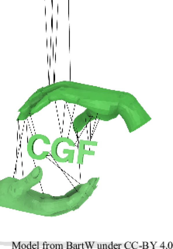
Figure 5: Wire-only solutions require support from above the arrangement’s center of mass.

3.3 Wires

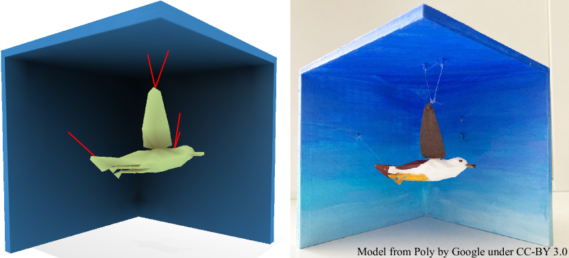
Figure 13: For a wire-only solution, we can save time by forgoing the visibility computation. Using fishing wire, we support the seagull in mid-air invisibly.

A special case of our model is a wire, which can be thought of as a tension-only rod. A wire $ij$ has zero resistance to bending and compression (i.e., $\sigma^{c}_{ij}=\sigma^{s}_{ij}=0$) and very high resistance to tension (i.e., $\sigma^{t}_{ij}>>0$). Wires made of strong material such as braided steel can be very thin (near invisible) while maintaining high strength. Our method will allow a mixture of tension-compression-bending rods (e.g., wooden dowels) and tension-only wires (steel wires), see Figure 9. As special case, we can limit our optimization to consider only wires, resulting in a hanging optimization (see Figures 5,13).

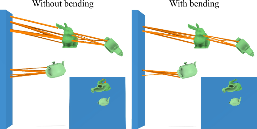
Figure 6: The addition of our linearized bending term yields sparser, less visible support structures by more accurately modelling the strength of the rods. Rods can also connect between objects rather than just to the support surface.

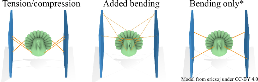
Figure 7: An enormous turkey levitates between two buildings using tension and compression resistant rods (left). Adding bending resistance affords a less voluminous solution (middle). Restricting the ground structure to only include edges perfectly intersecting the center of mass $(^{*})$ admits a bending only solution (right).

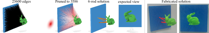
Figure 8: Our method constructs a over-connected ground structure of candidate edges (left) then immediately prunes edges that intersect the scene (middle) and finally extracts a small number of hidden rods. Savings from pruning can produce $10\times$ performance improvements.

3.4 Visibility

We define the expected visibility of a rod as function of the input viewpoint distribution, occlusions due to the scene, the rod’s position and orientation and its unknown cross-sectional area. For a rod $ij$, its expected visibility $v_{ij}$ is:

$$v_{ij} =\int_{\mathcal{E}}p(\mathbf{e})\int_{C_{ij}}r(\mathbf{e},\mathbf{x})\;d\Omega\;d\mathbf{e},$$ (6)

where

$$r(\mathbf{e},\mathbf{x}) =\begin{cases}0&\text{if the segment $\mathbf{e}\mathbf{x}$ intersects the scene},\\ 1&\text{otherwise},\end{cases}$$

where $\mathcal{E}$ defines the set of viewpoints and $p(\mathbf{e})$ is the probability density associated with the point $\mathbf{e}\in\mathcal{E}$, and $C_{ij}$ is the surface of the cylindrical rod with cross-sectional area $a_{ij}$ connecting endpoints $\mathbf{x}_{i}$ and $\mathbf{x}_{j}$, and $d\Omega$ is the differential solid angle at the corresponding integration point $\mathbf{x}$ subtended at the viewpoint $\mathbf{e}$. Measuring visibility according to solid angle correctly matches the intuition that the same size rod farther away from an observer is less visible.

The outer integral is immediately recognizable as a soft-shadow or area-light source evaluation common in rendering. We can approximate this well by Monte-Carlo importance sampling over the viewpoint distribution. An analytic expression for the inner integral becomes unwieldy, so we instead opt for a simple approximation based on uniform quadrature, accounting for the orientation of the rod resulting in foreshortened projection. Rods are thin relative to the scene and spread of the viewpoint distributions, therefore we assume visibility to be constant in the normal directions of the rod. Our discrete approximation of the expected visibility is thus a double sum over $n_{u}$ points sampled according to the input probability density function and $n_{ij}$ points sampled along the rod:

$$v_{ij} \approx\sqrt{a_{ij}}\underbrace{\frac{1}{n_{u}\sqrt{2\pi}}\sum_{u=1}^{n_{u}}\cos^{-1}\left(\frac{(\mathbf{x}_{i}-\mathbf{e}_{u})\cdot(\mathbf{x}_{j}-\mathbf{e}_{u})}{\|\mathbf{x}_{i}-\mathbf{e}_{u}\|\|\mathbf{x}_{j}-\mathbf{e}_{u}\|}\right)\sum_{w=1}^{n_{ij}}r(\mathbf{e}_{u},\mathbf{x}_{w})}_{g_{ij}},$$

where we collect the terms that do not depend on $a_{ij}$ into a single non-negative scalar per-rod, $g_{ij}\in\mathbb{R}_{\geq 0}$. In this way, the squared visibility of each rod becomes a linear function of the cross-sectional area: $a_{ij}g_{ij}^{2}$. Because wires are so thin compared to rods, we happily set $g_{ij}=0$ for wires and avoid their visibility precomputation. To generate the $n_{ij}$ samples on edge $ij$, we subdivide the edge until all segments are less than a given scene-dependent length threshold (e.g., $0.1$ meters for the bedroom scene in Figure Levitating Rigid Objects with Hidden Rods and Wires) and then use the segment barycenters as samples (typically 10-100 samples per edge). Segment queries can be computed in parallel.

3.5 Ground Structure

The space of physically feasible supporting structures is high-dimensional and a mixture of discrete variables (e.g., how many rods? connecting between which objects?) and continuous variables (e.g., where rods attach to each object? what are the rod thicknesses?). Navigating this space to find a globally optimal solution is difficult. In response, the ground structure method (e.g., [Dor64, Ped93, ZP15, Fre04] makes the problem tractable by rephrasing the problem into selecting a discrete subset of support elements from an intentionally dense yet finite set of candidate elements. This candidate set is referred to as the “ground structure.”

In our case, we generate a ground structure of candidate rod and wire elements by Poisson disk sampling [Yuk15] all rigid objects and the support surface and then connecting all possible pairs of points from different sources (e.g, for a single rigid object this forms a bipartite graph with the supporting surface, see Figure 8). For each edge in this graph, we label it as a “rod” or “wire” (and possibly create duplicate copies so edges appear as both types). We can discard a bad edge $ij$ if its attachment angle is self-penetrating or too obtuse (by checking if the rod vector dotted with the surface normal is below a threshold; $\hat{\mathbf{t}}_{ij}\cdot\hat{\mathbf{n}}_{i}<\cos\theta_{\text{max}}$), if it intersects objects in the scene (by ray casting), or if its computed visibility coefficient is exceptionally high ($g_{ij}>g_{\text{max}}$). We refer to the result as the pruned ground structure $\mathcal{G}$.

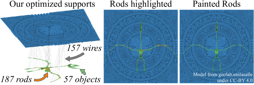
Figure 9: We show the rods in orange to demonstrate how hidden they are. But we show that the rods connecting the smaller parts (middle) can be painted to blend in with the ceiling (right).

3.6 Sparse Optimization

The beauty of the ground structure method is that once the candidate set has been chosen, selecting the globally optimal subset can be phrased as an efficient convex optimization, in particular a linear program. In the classic method, the cost function to be minimized is the total volume of material spent on the support structure. Since all edge lengths are known once the candidate set is selected, this cost is a linear function of the yet unknown edge cross-sectional areas. It is important that this cost function is the unsquared volume, which can be thought of as the L1-norm of the vector of edge areas (weighted by edge-lengths), as opposed to the sum of squared per-edge volumes, analogous to the L2-norm. The L1-norm is sparsity inducing and under mild conditions will agree with the optimal solution of the selection problem, analogous to the L0-pseudonorm  [CWB08, FMP*13]. As a result, the vast majority of edges in the solution will have exactly zero area.

In our case, we augment the total volume cost function with a least-squares visibility term to penalize choosing highly visible rods. Because our per-edge visibility measurement in Eq. 3.4 is linear in the square-root of the rod areas, this least-squares energy becomes linear in the areas.

The areas of the rods and wires are the primary unknowns. We introduce auxiliary variables $c_{ij}$ and $\mathbf{q}_{ij}$ as described in Sec. 3.2 to facilitate writing our force and torque balance constraints (see Sec. 3.1). These variables are then coupled to the areas via the yield stress inequalities (see Eq. 5).

The resulting optimization is a linear program over the pruned ground structure $\mathcal{G}$ containing $m$ candidate edges:

$$\mathop{\text{min}}_{\mathbf{a},\mathbf{c},\mathbf{q}} \sum_{ij\in\mathcal{G}}a_{ij}(\ell_{ij}+\lambda g_{ij}^{2})$$ (7)

s.t. $$\sum_{ij|j\in V_{k}}c_{ij}\hat{\mathbf{t}}_{ij}+{\mathbf{N}}_{ij}\mathbf{q}_{ij}=m_{k}\mathbf{g},\;\forall\;k=1,\dots,K$$ (8)

$$\sum_{ij|j\in V_{k}}(c_{ij}\hat{\mathbf{t}}_{ij}+{\mathbf{N}}_{ij}\mathbf{q}_{ij})\times(\mathbf{x}_{j}-\overline{\mathbf{x}}_{k})=0,\;\forall\;k=1,\dots,K$$

$$-\sigma_{ij}^{c}a_{ij}\leq c_{ij}\leq\sigma_{ij}^{t}a_{ij},\;\forall\;ij\in\mathcal{G}$$ (9)

$$-\sigma_{ij}^{s}a_{ij}\leq\mathbf{q}_{ij}\leq\sigma_{ij}^{s}a_{ij},\;\forall\;ij\in\mathcal{G}$$ (10)

$$a_{ij}\geq 0,\;\forall\;ij\in\mathcal{G}$$ (11)

where we stack all $a_{ij}$, $c_{ij}$, and $\mathbf{q}_{ij}$ variables into vectors $\mathbf{a}\in\mathbb{R}^{m}$, $\mathbf{c}\in\mathbb{R}^{m}$, and $\mathbf{q}\in\mathbb{R}^{2m}$, respectively, and we introduce the user-controllable weighting term $\lambda$ to balance between preference for volume and visibility minimization. For all examples shown, we use $\lambda$ = 10,000.

We opt to replace the second-order cone constraint for linearized bending yields in Eq. 5 with the simpler coordinate-wise linear inequality in Eq. 10. This can be thought of as a conservative $L_{\infty}$ approximation, and albeit coordinate system dependent, does not affect results and admits a faster linear program than a conic program in our experience.

The linear coefficients in the force/torque balance equations and linear inequalities (Eqs. 8-10) can be collected in large sparse matrices (see App. Appendix: Matrix Form). Many efficient solvers exist for such large sparse linear programs; we use Mosek [AA00].

A solution is a guaranteed to exist as long as force and torque balance can be achieved. This could fail to happen for very sparse ground structures (e.g., less than six edges per object) or degenerate situations (e.g., all edges are parallel). Our very dense ground structure (hundreds of thousands of edges) enjoys the general position of its random providence. We never fail to find a feasible solution.

4 Experiments & Results

Scene	$K$	full	$m$	time	$R$	$W$
Parade Float	1	20K	10K	0.14	0	12
“Koons” Display	1	154K	22K	4.90	2	4
Ghost With Tail	1	11K	1K	5.01	5	0
Bunny/Teapot/Rocker	3	150K	21K	2.04	16	0
Bedroom	13	490K	46K	35.87	41	35
Zoetrope (1 frame)	1	469K	51K	33.77	4	0
Pterosaurus	57	10M	785K	608.01	187	157

Table 1: Timings in seconds (time) and numbers of rods ($R$) and wires ($W$) for each result with $K$ objects. full and $m$ are edges in the original and pruned ground structures, respectively. The “Pterosaurus” and “Parade Float” examples do not include the time for computing visibility, as it was not used in the LP objective.

We implemented our algorithm in Matlab using gptoolbox [Jac*18] for geometry processing and Mosek [AA00] to solve the linear program formulated in Section 3.6. Pre-computation of the integrated visibility, in our input scene is accelerated using the Embree [WWB*14] ray-tracer as interfaced by libigl [JP*20]. We report statistics and timings for the results in our paper in Table 1. All times are reported on a MacBook Pro with 3.5 GHz Intel Core i7 and 16GB of RAM. Visibility pre-computation is computed in parallel, but is still typically the bottleneck ($\approx 80\%$).

The number of degrees of freedom in the system is the size of the ground structure which generally scales quadratically in the number of objects $m=O(K^{2})$, typically generated by taking all inter-object pairs over 10-100 Poisson disk sample points on each object. The inset graph shows the effect of increasing the degrees of freedom on Figure 4. While optimization time increases linearly with degrees of freedom, improvement to the visibility score of the solution reaches a point of diminishing return.

Starting with a dense ground structure leads to better qualitative results, but the exact positions of the samples do not drastically effect the hidden-ness of the result. Figure 11 shows how little the solution changes as a function of the ground structure sampling.

Pruning often significantly reduces the ground structure size and consequently, the number of degrees of freedom (see, e.g., Figure 8). Perhaps unsurprisingly, we typically experience a speedup the same ratio of original ground structure edges to pruned ground structure edges. The number of constraints in our optimization is six times the number of objects $K$. After pruning, Mosek finds a solution for the above problem configuration within a few minutes.

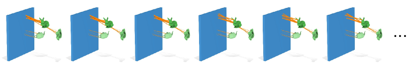
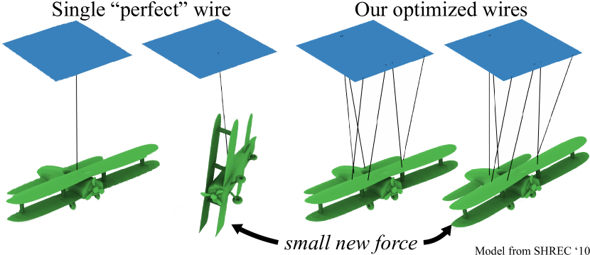
Figure 10: Our results depend on a randomly generated ground structure. Changing the random seed affects the precise result, but not qualitatively.

Figure 11: Applying a small new force to the plane held by a single wire causes undesired behaviour since a single wire attachment is not enough to balance the torque. Our method gives a 6-wire solution, exactly the number needed to balance force and torque.

In our accompanying video, we show animations of results in this paper including traversals of the viewing distributions to demonstrate the robustness of our methods ability to hide supports.

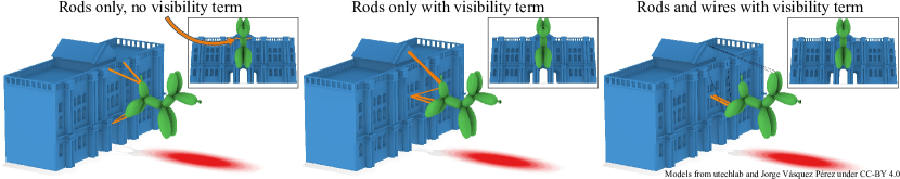
Figure 12: Applying the ground structure method to this example of a giant balloon hanging outside of a museum gives sufficient rods to support it, but they are visible. Using our visibility term in the optimization yields a support structure with rods hidden to the viewpoints. Allowing wires for tension and rods for compression, the result is a few thick but invisible rods and thin wires which hold the balloon in place.

Levitating 3D objects has a wide range of applications including scientific visualization, film and theater set design, home decor, anamorphic 3D art installations, as well as objects for zoetropes and 3D stop-motion animation. Each application has specific design requirements, and our algorithm is designed to enable the exploration of a number of aesthetic and structural parameters and design choices, which significantly impact the resulting solution. We elaborate on some of these design use cases.

Both scientific exhibits (see, e.g., Figures Levitating Rigid Objects with Hidden Rods and Wires,1) and illusory art installations (see Figure 14) require an unobscured view of the levitating objects. While it is feasible for designers to hand-craft support structures from a single fixed viewpoint, the interplay between visibility and structural stability is quite complex for mutli-view distributions. In Figure Levitating Rigid Objects with Hidden Rods and Wires, we show the ability of our algorithm to adapt its optimal solution to multiple viewpoint distributions.

Our algorithm is able to holistically optimize the support structure using a mix of rods and wires. We color our rods bright orange for evaluation in this paper, but in practice they can be further camouflaged by matching their appearance to the background or scene objects (see Figures 9,15). The choice of using a rod or wire is both aesthetic (as determined by a user) and functional. For example, supporting a levitating object with a wire would require a potential attachment points on the fixed surface or other levitating objects, to be vertically higher than the given object (see, e.g., Figure 5). The inset figure shows a parade float suspended by optimized wires (the net force pointing upward due to buoyancy). Previous methods have considered hanging objects [PWLS13] or more generally mobiles [MML16] by placing a single support “perfectly” placed in alignment above the center of mass. While this strategy requires the fewest supports, it is an unstable solution (see Figure 11). Our method relies on random sampling of points in general position, typically producing multiple wires per hanging object, but resulting in a more stable configuration. Thus, in practice, we’ve found both our 3D printed and assembled results to be quite resilient to outside forces (including those from falls, heavy winds, and moving from one place to another).

Mounting objects off the side of a support such as a wall is best achieved with a mixture of wires and rods. Figure 12 shows a giant promotional display suspended in front of a contemporary art museum. We provide a symmetric dense ground structure and our optimization naturally finds a symmetric sparse solution.

The pterosaurus in Figure 9 has 57 separate bones and requires a complex support structure, acting as a stress test on our optimization. In practice, skeleton displays often pre-plaster-fuse bones to reduce the number of pieces (see spine of whale in Figure 1).

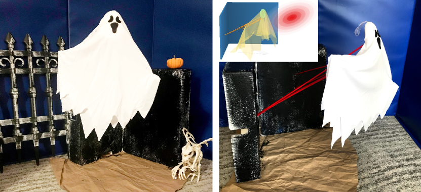
Figure 14: The model used for support attachments does not have to be the same one used for visibility. The ghost’s head (green) has attached supports, while its tail (yellow) hides them.

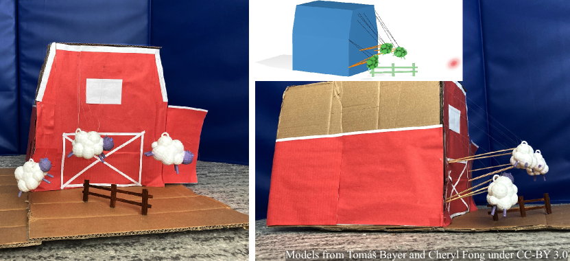
Figure 15: By maintaining separate graphs for rods and wires, we can use differing visibility weights and yield stresses based on what materials are going to be used in fabrication. Our system can wisely select which edges should be wires vs rods.

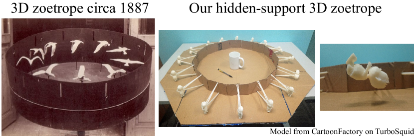
Figure 16: 3D zoetropes are an old idea, but hiding supports for flying objects is still challenging. We incorporate the centripetal force due to spinning and hide supports behind a backflipping boy zoetrope. See accompanying video at 3m20s.

The idea of stop-motion animation and 3D zoetropes is over a century old [Mar90], with modern examples including “Feral Fount” by Gregory Barsamian at the Museum of the Moving Image in Queens and the Toy Story zoetrope featured in Pixar’s Museum Exhibit. The portrayal of levitating objects in this medium is particularly challenging. We demonstrate a prototypical result of a backflipping boy in Figure 16 by hiding supporting rods out of sight. For this example to be structurally stable both at rest and while spinning, we first find the optimal set of rods for each frame under gravity and then re-run the linear program on just these rods subject to centripetal forces. The final rod thickness are the maximum over the two solves. Incorporating more elaborate multi-load handling (cf. [Fre04]) is left as future work.

5 Limitations & Future Work

Our rod model includes linearized tension, compression, and bending forces. Like many past methods, we do not handle the self-weight of the rods by assuming that the force of gravity is much larger than the force of the rods on themselves. This is a trivial addition of gravity forces on each rod proportional to their length. Ground structure methods may produce solutions where thickened rods intersect; ours is no exception. Edges which nearly overlap with each other appear in the original ground structure and therefore may be selected as rods in the solution. However, this has not caused any fabrication problems in practice. Previous methods have considered penalty terms or post-pressing to deal with intersecting (e.g., [JTSW17]). Wire-wire intersections are extremely unlikely due to the very thin nature of wires. Our visibility model considers direct line of sight, but not other cues such as reflections or shadows. Transparency of objects is not accounted for. Depending on the setup of the scene, there may not be a solution invisible to every viewpoint (e.g., Figure 17). Since we model physical validity as a hard constraint, we are still able to find a solution, albeit a visible one.

The precise solution depends on the initial ground structure. In general, denser ground structures produce higher quality solutions — both in terms of total structure volume and hidden-ness — with diminishing returns. Rod areas are directly proportional to stress limits, so acurate fabrication relies on accurate (or at least conservative) material measurement.

Our algorithm assumes that the input is a well-crafted scene to begin with and leaves it perfectly as inputted. The creative design process for these scenes is itself non-trivial. In the future, we are interested in pursuing an interactive design tool which would provide hints to increase occlusion by applying simple transformations (translations, rotations and scales) to the objects in the scene or even provide automatic layout optimizations given the objects and the viewpoints.

We model the problem of hidden supports as an efficient linear program that leverages fast ray-casting from computer graphics. We see an exciting future in combining techniques from rendering and geometry processing with structural optimization in architecture and engineering. We hope this combination of appearance-driven design will be beneficial to scientific and artistic endeavours.

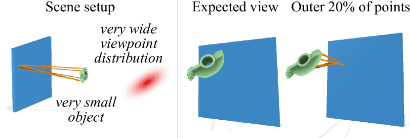
Figure 17: In the case of a very wide viewpoint distribution and a small or thin object, there will most likely be viewpoints from which the supports are visible. The rightmost figure shows the scene from a viewpoint on the outer 20% of the distribution.

6 Acknowledgements

This research is funded by New Frontiers of Research Fund (NFRFE–201), NSERC Discovery (RGPIN2017–05235, RGPAS–2017–507938), the Ontario Early Research Award program, the Canada Research Chairs Program, the Fields Centre for Quantitative Analysis and Modelling and gifts by Adobe Systems, Autodesk and MESH Inc. We would like to thank Michael Tao, Silvia Sellán and Rinat Abdrashitov for proofreading; John Hancock for IT and fabrication hardware support; the anonymous reviewers for their helpful comments.

Appendix: Matrix Form

Solvers like Mosek [AA00] expect the problem to be provided in matrix form. We spell out the coefficients of the relevant sparse matrices implementing the linear program in Eq. 8.

For our pruned ground structure with $m$ candidate edges connecting $N$ vertices, introduce a unit-less sparse matrix $\mathbf{C}\in\mathbb{R}^{3N\times m}$ where:

$$\mathbf{C}_{jl}=\begin{cases}\hphantom{-}\hat{\mathbf{t}}_{ij}&\text{ if rod $ij$ points toward $\mathbf{x}_{j}$ }\\ -\hat{\mathbf{t}}_{ij}&\text{ if rod $ij$ points away from $\mathbf{x}_{j}$ }\\ \hphantom{-}0&\text{ otherwise.}\end{cases}$$ (12)

Here, $j$ is used to index the 3 rows that correspond to the vertex $\mathbf{x}_{j}$ and $l$ is used to index the column for rod $ij$.

Introduce a unit-less sparse matrix $\mathbf{Q}\in\mathbb{R}^{3N\times 2m}$ where

$$\mathbf{Q}_{jl}=\begin{cases}\hphantom{-}\hat{\mathbf{N}}_{ij}&\text{ if rod $ij$ points toward $\mathbf{x}_{j}$ }\\ -\hat{\mathbf{N}}_{ij}&\text{ if rod $ij$ points away from $\mathbf{x}_{j}$ }\\ \hphantom{-}0&\text{ otherwise.}\end{cases}$$ (13)

Introduce a sparse unit-less selection matrix $\mathbf{S}\in\mathbb{R}^{3K\times 3N}$, where

$$\mathbf{S}_{kj}=\begin{cases}I_{3}&\text{ if vertex $\mathbf{x}_{j}$ lies on object $k$}\\ 0&\text{ otherwise}\end{cases}$$ (14)

Introduce a sparse cross-product matrix $\mathbf{D}\in\mathbb{R}^{3K\times 3N}$ with units meters, where

$$\mathbf{D}_{kj}=\begin{cases}[\mathbf{x}_{j}-\overline{\mathbf{x}}_{k}]_{\times}&\text{ if vertex $\mathbf{x}_{j}$ lies on object $k$}\\ 0&\text{ otherwise}\end{cases}$$ (15)

where

$$[\mathbf{d}]_{\times}=\begin{bmatrix}0&-\mathbf{d}_{3}&\mathbf{d}_{2}\\ \mathbf{d}_{3}&0&-\mathbf{d}_{1}\\ -\mathbf{d}_{2}&\mathbf{d}_{1}&0\end{bmatrix}\in\mathbb{R}^{3\times 3}$$ (16)

Finally, the full linear program in matrix form may be written

$$\mathop{\text{min}}\limits_{\mathbf{a},\mathbf{c},\mathbf{q}} \quad{(\ell+\lambda g^{\prime})}^{\top}\mathbf{a}$$ (17)

subject to $$\quad\begin{bmatrix}\mathbf{0}&\mathbf{S}\mathbf{C}&\mathbf{S}\mathbf{Q}\\ \mathbf{0}&\mathbf{D}\mathbf{C}&\mathbf{D}\mathbf{Q}\end{bmatrix}\begin{bmatrix}\mathbf{a}\\ \mathbf{c}\\ \mathbf{q}\end{bmatrix}=\begin{bmatrix}\mathbf{m}\otimes\mathbf{g}\\ 0\end{bmatrix}$$ (18)

and $$\quad-\sigma_{t}\mathbf{a}_{l}\leq\mathbf{c}_{l}\leq\mathbf{a}_{l}\sigma_{c},\forall l$$ (19)

and $$\quad-\sigma_{s}\mathbf{a}_{l}\leq\mathbf{q}_{l}\leq\mathbf{a}_{l}\sigma_{s},\forall l.$$ (20)

where $g^{\prime}_{l}=g_{l}^{2},\hskip 2.84526pt\forall l$ since the squared visibility is linear in the cross-sectional areas of each rod.

$\mathbf{m}\otimes\mathbf{g}$ denotes the Kronecker product of the $\mathbf{m}\in\mathbb{R}^{K}$ stacked vector of object masses and the $\mathbf{g}\in\mathbb{R}^{3\times 1}$ gravity vector.

References

- [AA00] E.. Andersen and K.. Andersen “The mosek interior point optimizer for linear programming: an implementation of the homogeneous algorithm” In High Performance Optimization, 2000
- [BWBS14] Moritz Bächer, Emily Whiting, Bernd Bickel and Olga Sorkine-Hornung “Spin-it: optimizing moment of inertia for spinnable objects” In ACM Trans. Graph., 2014
- [CW96] Robert Connelly and Walter Whiteley “Second-Order Rigidity and Prestress Stability for Tensegrity Frameworks” In SIAM J. Discrete Math., 1996
- [CWB08] Emmanuel J Candes, Michael B Wakin and Stephen P Boyd “Enhancing sparsity by reweighted l1 minimization” In Journal of Fourier analysis and applications Springer, 2008
- [CZS*19] Subramanian Chidambaram et al. “Shape Structuralizer: Design, Fabrication, and User-driven Iterative Refinement of 3D Mesh Models” In Proc. CHI, 2019
- [CZT16] Stelian Coros, Jonas Zehnder and Bernhard Thomaszewski “Designing structurally-sound ornamental curve networks” In ACM Trans. Graph., 2016
- [DFL*15] Harish Doraiswamy et al. “Topology-based catalogue exploration framework for identifying view-enhanced tower designs” In ACM Trans. Graph., 2015
- [Dor64] W Dorn “Automatic design of optimal structures” In J. de Mecanique, 1964
- [DPW*14] Mario Deuss et al. “Assembling self-supporting structures” In ACM Trans. Graph., 2014
- [FLM*20] Laccone Francesco et al. “Automatic Design of Cable-Tensioned Glass Shells” In Comput. Graph. Forum, 2020
- [FMP*13] Mingbin Feng et al. “Complementarity formulations of l0-norm optimization problems” In Industrial Engineering and Management Sciences. Technical Report. Northwestern University, Evanston, IL, USA, 2013
- [Fre04] Robert M. Freund “Truss Design and Convex Optimization”, 2004
- [HHC18] Kai-Wen Hsiao, Jia-Bin Huang and Hung-Kuo Chu “Multi-view Wire Art” In ACM Trans. Graph., 2018
- [HZH*16] Yijiang Huang et al. “FrameFab: robotic fabrication of frame shapes” In ACM Trans. Graph., 2016
- [Jac*18] Alec Jacobson “gptoolbox: Geometry Processing Toolbox” http://github.com/alecjacobson/gptoolbox, 2018
- [Jac19] Alec Jacobson “RodSteward: A Design-to-Assembly System for Fabrication using 3D-Printed Joints and Precision-Cut Rods” In Comput. Graph. Forum, 2019
- [JP*20] Alec Jacobson and Daniele Panozzo “libigl: A simple C++ geometry processing library” http://libigl.github.io/libigl/, 2020
- [JTSW17] Caigui Jiang, Chengcheng Tang, Hans-Peter Seidel and Peter Wonka “Design and volume optimization of space structures” In ACM Trans. Graph., 2017
- [KSW*17] Robert Kovacs et al. “TrussFab: Fabricating Sturdy Large-Scale Structures on Desktop 3D Printers” In Proc. CHI, 2017, pp. 2606–2616
- [LGC*18] Jikai Liu et al. “Current and Future Trends in Topology Optimization for Additive Manufacturing” In Struct. Multidiscip. Optim., 2018
- [Mar90] E.J. Marey “Physiologie du mouvement: vol des oiseaux”, 1890
- [MKS*17] Vittorio Megaro et al. “Designing cable-driven actuation networks for kinematic chains and trees” In Proc. SCA, 2017
- [MML16] Liane Makatura, Catherine Most and Gloria Li “Balancing Act: An Interactive Tool for Fabricating Calder-Style Hanging Mobiles”, Technical Report Dartmouth College, 2016
- [MP09] Niloy J. Mitra and Mark Pauly “Shadow Art” In ACM Trans. Graph., 2009
- [Ped93] Pauli Pedersen “Topology optimization of three-dimensional trusses” In Topology design of structures Springer, 1993, pp. 19–30
- [PTC*15] Jesús Pérez et al. “Design and fabrication of flexible rod meshes” In ACM Trans. Graph., 2015
- [PTV*17] Nico Pietroni et al. “Position-based tensegrity design” In ACM Trans. Graph., 2017
- [PWLS13] Romain Prévost, Emily Whiting, Sylvain Lefebvre and Olga Sorkine-Hornung “Make it stand: balancing shapes for 3D fabrication” In ACM Trans. Graph., 2013
- [SPS14] Christian Schüller, Daniele Panozzo and Olga Sorkine-Hornung “Appearance-mimicking Surfaces” In ACM Trans. Graph., 2014
- [STTP14] Yuliy Schwartzburg, Romain Testuz, Andrea Tagliasacchi and Mark Pauly “High-contrast Computational Caustic Design” In ACM Trans. Graph., 2014
- [SVB*12] Ondrej Stava et al. “Stress relief: improving structural strength of 3D printable objects” In ACM Trans. Graph., 2012
- [VHWP12] Etienne Vouga, Mathias Höbinger, Johannes Wallner and Helmut Pottmann “Design of self-supporting surfaces” In ACM Trans. Graph., 2012
- [WDW16] Jun Wu, Christian Dick and Rüdiger Westermann “A System for High-Resolution Topology Optimization” In IEEE Trans. Vis. Comput. Graph., 2016
- [WWB*14] Ingo Wald et al. “Embree: a kernel framework for efficient CPU ray tracing” In ACM Trans. Graph., 2014
- [WWY*13] Weiming Wang et al. “Cost-effective printing of 3D objects with skin-frame structures” In ACM Trans. Graph., 2013
- [Yuk15] Cem Yuksel “Sample Elimination for Generating Poisson Disk Sample Sets” In Proc. Eurographics, 2015
- [ZHMB20] Tomás Zegard, Christian Hartz, Arek Mazurek and William F. Baker “Advancing building engineering through structural and topology optimization” In Structural and Multidisciplinary Optimization, 2020
- [ZLP*15] Xiaoting Zhang et al. “Perceptual models of preference in 3D printing direction” In ACM Trans. Graph., 2015
- [ZP15] Tomás Zegard and Glaucio H Paulino “GRAND3: Ground structure based topology optimization for arbitrary 3D domains using MATLAB” In Structural and Multidisciplinary Optimization, 2015
- [ZPZ13] Qingnan Zhou, Julian Panetta and Denis Zorin “Worst-case structural analysis” In ACM Trans. Graph., 2013