Direct geometrical measurement of the Hubble constant from galaxy parallax: predictions for the Vera C. Rubin Observatory and Nancy Grace Roman Space Telescope

Abstract

We investigate the possibility that a statistical detection of the galaxy parallax shifts due to the Earth’s motion with respect to the CMB frame (cosmic secular parallax) could be made by the Vera C. Rubin Observatory Legacy Survey of Space and Time (LSST) or by the Nancy Grace Roman Space Telescope (NGRST), and used to measure the Hubble constant. We make mock galaxy surveys which extend to redshift $z=0.06$ from a large N-body simulation, and include astrometric errors from the LSST and NGRST science requirements, redshift errors and peculiar velocities. We include spectroscopic redshifts for the brightest galaxies ($r<18$) in the fiducial case. We use these catalogues to make measurements of parallax versus redshift, for various assumed survey parameters and analysis techniques. We find that in order to make a competitive measurement it will be necessary to model and correct for the peculiar velocity component of galaxy proper motions. It will also be necessary to push astrometry of extended sources into a new regime, and combine information from the different elements of resolved galaxies. In an appendix we describe some simple tests of galaxy image registration which yield relatively promising results. For our fiducial survey parameters, we predict an rms error on the direct geometrical measurement of $H_{0}$ of $2.8\%$ for LSST and $0.8\%$ for NGRST.

1 Introduction

There has been much recent evidence for tension between different measurements of the Hubble constant (e.g., Freedman et al., 2019; Riess, 2019). Discrepancies between local and early Universe measurements (Verde et al., 2019) have been interpreted by some as evidence for problems with the standard cosmological model. On the other hand, it is indisputably difficult to measure cosmological distances, as shown by the history of Hubble constant measurements (e.g., Huchra, 1992; Croft & Dailey, 2011; Crossland et al., 2020). It is clear that new techniques would be helpful, and in principle the more direct the better. Most basic would be to use geometry: parallax measurements, but so far these have only been used for distances within our galaxy. The baseline for annual parallax is a limiting factor in this case. An alternative for observing parallax shifts of objects beyond our galaxy is the continually increasing baseline caused by the Earth’s motion with respect to CMB frame (Kardashev et al., 1973; Ding & Croft, 2009, hereafter DC). This cosmic secular parallax could be detected by the Gaia satellite (DC, Paine et al. 2020; Hall 2019), but the LSST offers a new opportunity, assuming that considerable difficulties with ground based astrometry can be overcome. Here we explore what might be possible in the best case scenario. We also explore what a future space based measurement with NGRST could offer.

There are many different methods used currently to measure the Hubble Constant, including supernovae and cepheids as standard candles (e.g., Dhawan et al., 2018; Riess et al., 2005; Riess, 2019; Freedman et al., 2001; Hubble, 1925), gravitational wave (GW) standard sirens (e.g., Holz & Hughes, 2005), gravitational lens (GL) time delay (e.g., Refsdal, 1966; Chen et al., 2019), and Baryon Acoustic Oscillations (BAO) in the CDM model as a standard ruler (e.g., Cuceu et al., 2019; Beutler et al., 2011). GW and GL probes are direct, without need for absolute calibration, but the modeling involved can be complex. The SN and Cepheids are rungs on the cosmic distance ladder, but not at the bottom, and so still need parallax measurements. So far, these annual parallax measurements are readily measurable out to $\sim 10\,{\rm kpc}$ (Brown et al., 2018; Lindegren et al., 2018; Bailer-Jones et al., 2018). To do better with space based observations new satellites have been proposed (e.g., Boehm et al., 2017). NGRST (see below) and Euclid (Sanderson et al., 2017; da Silva et al., 2019), which are more general telescopes will also have great astrometry potential.

The Nancy Grace Roman Space Telescope (NGRST, formerly known as WFIRST Spergel et al. 2013) is a NASA observatory designed to use wide field imaging and slitless spectroscopy to study a range of topics including dark energy, exoplanets and infrared astrophysics. The satellite’s Wide-Field Instrument (WFI) provides a sharp point spread function, precision photometry, and stable observations. The field of view is 0.28 square degrees, allowing efficient coverage of large regions of the sky. A primary mission lifetime of 5 years (with a possible extension to 10) will provide a baseline for measurement of proper motions, and the dataset promises to be a superb astrometric resource. The currently planned launch date is 2025.

The Vera Rubin Observatory is an almost completed ground based observatory(Starr et al., 2002; Tyson et al., 2003) which will survey the entire southern hemisphere every few nights for 10 years (Marshall et al., 2017) to carry out the Legacy Survey of Space and Time (LSST). While ground based, the LSST is planned to have excellent photometry with unsurpassed time domain qualities, relevant to $H_{0}$ measurement (e.g., for variable stars, SN, the quasar variability needed for GL time delay). The astrometry carried out by the telescope will also lead to an enormous dataset, with billions of objects measured (Graham, 2019; Abell et al., 2009). For the purposes of this paper, for both NGRST and the LSST, we are most concerned with the relative astrometry between distant quasars/galaxies and those within a few hundred Megaparsecs. This is because we are interested in cosmic secular parallax.

Cosmic parallax (Kardashev et al., 1973; Ding & Croft, 2009) is one of the possible observables in the field of ”real time cosmology” (Quercellini et al., 2012; Darling, 2012; Darling & Truebenbach, 2018; Korzyński & Kopiński, 2018). Other examples are the redshift drift (Sandage, 1962; Loeb, 1998), the real time change in CMB anisotropies (Lange & Page, 2007), or the CMB temperature (Abitbol et al., 2020). One could imagine others e.g., a time varying Tolman test (Tolman, 1934) etc., but it is clear that many ideas are futuristic at best. Neverthless, there appears to be an interesting path forward for some of these observables. Pioneering work to set current limits has been carried out by Darling (2012), for redshift drift from 21cm radio observations, and Paine et al. (2020) for cosmic parallax from Gaia.

Large new facilities (e.g., Rubin Observatory, NGRST) can be used to carry out precision cosmology using well tested probes (e.g., Chisari et al., 2019) but also may be able to detect more futuristic effects such as those from real time cosmology. The latter may perhaps even be carried out with the accuracy required to make competitive constraints. They may also yield surprises, which could be their most interesting aspect.

Our plan for this paper is as follows. In Section 2, we review the concept of cosmic secular parallax. In Section 3 we describe our mock Rubin Observatory LSST and NGRST surveys, including a brief introduction to the Rubin Observatory and NGRST, the cosmological Nbody simulations we use, and how we include various observational effects in the mocks. In Section 4 we describe how we we measure the secular parallax as a function of redshift from the mock surveys. In Section 5 we explain how we determine the estimated error on $H_{0}$ measurements, and show how the error depends on survey parameters and variations in the analysis techniques. In Section 6 we summarise our conclusions and discuss the possible ways forward. In Appendix A, we describe some simple test measurements of galaxy image shifts using observational data.

2 Cosmic parallax

Unlike the annular parallax, which repeats at a constant (small) value, the Earth’s motion with respect to the CMB provides a much longer usable baseline for parallax measurements. This latter effect is a variant of the “secular” parallax (see e.g., Binney & Merrifield, 1998, Section 2.2.3), and is in principle easier to measure because the signal increases linearly with time. Kardashev et al. (1973) were the first to propose the cosmic version of the secular parallax as a means for measuring distances outside our galaxy. DC revisited the idea of this cosmic parallax in the era of modern CMB measurements and the CDM cosmological model. Paine et al. (2020) were the first to use observational data to try to measure the effect, using Gaia Data Release 2 to find an upper limit, although this was still a factor of $\sim 40$ above the prediction (see below).

The parallax distance to an object in an expanding Universe was first calculated theoretically in the context of the usual annual parallax and published by McCrea (1935). Not suprisingly, he noted that it was unlikely to be measurable. It appears also in the textbook by Weinberg (1972). The solar system is moving with respect to the CMB frame at a velocity of $369\pm 0.9\,{\rm km}\,{\rm s}^{-1}$ towards an apex with galactic latitude and longitude $l=263.99^{\circ}\pm 0.14^{\circ},b=48.26^{\circ}\pm 0.05^{\circ}$ (Kogut et al., 1993; Hinshaw et al., 2009; Akrami et al., 2020) As a result, all extragalactic objects will experience a parallax shift, increasing linearly with time, towards the antapex with amplitude proportional to $\sin\beta$, where $\beta$ is the angle between the object and the direction of the apex. Over the observing period of the LSST (or extended NGRST mission), a baseline constantly increasing to $l=3800\mu\rm{pc}$ after ten years is therefore available for measures of parallax. This leads to a maximum apparent proper motion of 77.8 $\mu$ arcsec yr^-1 for galaxies at a 90 deg. angle to the apex. We summarize below the expressions for the parallax shift of a distant extragalactic source (first computed by McCrea 1935), using the notation due to Kardashev et al. (1973) and Hogg (1999).

The equation for the parallax angle $\theta$ is given by:

$$\theta=\frac{\ell}{r}$$ (1)

where $\ell$ is the baseline. Here $r$ is the comoving parallax distance, dependent on the curvature of the Universe in the following manner:

$$r=\left\{\begin{array}[]{ll}\frac{c}{H_{0}}\frac{1}{\sqrt{\Omega_{k}}}\tanh(\frac{\sqrt{\Omega_{k}}H_{0}}{c}D)&\Omega_{k}>0\\ D&\Omega_{k}=0\\ \frac{c}{H_{0}}\frac{1}{\sqrt{|\Omega_{k}|}}\tan(\frac{\sqrt{|\Omega_{k}|}H_{0}}{c}D)&\Omega_{k}<0\end{array},\right.$$ (2)

where

$$D=c\int^{z}_{0}\frac{dz^{\prime}}{H(z)}.$$ (3)

Here $\Omega_{k}$ is the curvature parameter expressed in terms of a fraction of the critical energy density. The parallax distance therefore resembles the angular diameter distance for a flat Universe, except that $r$ is a comoving rather than proper distance. In the present paper, we restrict all our analysis to extremely nearby galaxies, with $z<0.06$. For simplicity, in our calculations we therefore assume Euclidean space, with $D=\frac{cz}{H_{0}}$, and $H(z)=H_{0}$ for all $z$ in our range of interest.

The parallax shift due to the changing baseline from the motion of the solar system will manifest itself as a proper motion, which is the observable we are interested in, and is given by

$$\lvert\pi\rvert=77.8\,r^{-1}\lvert\sin{\beta}\rvert\,\mu\,{\rm arcsec\,yr}^{-1}\,{\rm Mpc},$$ (4)

where the angle $\beta$ is as defined above.

3 Mock observations

We use cosmological Nbody simulations to construct simple mock astrometry surveys of nearby galaxies, adding cosmological parallax as well as other physical and observational effects. We choose the Vera Rubin Observatory’s primary dataset, LSST and the Roman Space Telescope HLS as two to simulate. The techniques are also applicable to other future surveys such those carried out by the Euclid satellite. We have not looked at synergy between LSST and HLS in this paper, but this might be something valuable to explore in future work.

3.1 The Vera C. Rubin Observatory Legacy Survey of Space and Time

The Vera C. Rubin Observatory is an astronomical observatory which will be carrying out an unprecedented survey of 18,000 sq. deg. of the southern hemisphere over the period 2022-2032. Approximately 2 million images will be taken over this 10 year period with a 3.2 gigapixel camera, leading to at least 100 Petabytes of data. The dataset (named the ”Legacy Survey of Space and Time”, LSST) will include time domain photometry for at least 25 billion galaxies, with better than 0.2 arcsecond pixel sampling. Each part of the sky will be visited approximately 825 times, with a (5 $\sigma$) magnitude limit in the stacked images of $r<27.8$.

The hundreds of images for each astronomical object will make the LSST an excellent resource for astrometry. The science requirements for LSST astrometry are detailed in Ivesić et al. (2018). The LSST is targeted to obtain parallax and proper-motion measurements of comparable accuracy to those of Gaia at its faint limit ($r<20$) and smoothly extend the error versus magnitude curve deeper by about 5 mag. We make use of the projected astrometric errors for LSST in our mock surveys (see Section 3.5 below), but with the considerable added assumption that it will be possible to carry out differential astrometry of extended objects (resolved galaxies).

3.2 The Nancy Grace Roman Space Telescope High Latitude Survey

After the launch of NGRST, a Wide Field Instrument (WFI) High-Latitude Survey (HLS) will be performed, taking up to 2 years of observations. The HLS will cover over 2,200 square degrees with imaging and low-resolution (grism) spectroscopy. The imaging, in four NIR bands ($Y$, $J$, $H$, and $F184$), will reach $J=26.7AB$ for point sources. The Y-band magnitude limit (which, for comparison is closest in wavelength to LSST $r$ band) will be 25.8. The slitless spectroscopy will measure redshifts for over 15 million sources at redshift 1.1 to 2.8. Imaging and spectroscopy will support dark energy weak lensing and baryon acoustic oscillation measurements, respectively, and form an invaluable survey for Guest Investigator archival research studies of general astrophysics topics. Astrometry will be one of these topics, and a detailed exploration of the capabilities of NGRST in this area is given by Sanderson et al. (2017).

As with LSST, we are making the assumption in this paper that astrometry of extended objects, namely galaxies, will be possible, and that the well resolved nature of nearby galaxies will allow more accurate measurements to be made than of single point sources. This will require new astrometric techniques, and this is briefly discussed in later sections of the paper.

Because the HLS covers a smaller fraction of the sky than the LSST, the orientation of the dataset with respect to the CMB dipole direction becomes important. The mean value of $\lvert\sin(\beta)\rvert$ over the NGRST HLS footprint is 0.3, where $\beta$ is angle between pixels and the dipole direction.

3.3 Simulations

We use the largest of the publicly available $\nu$²GC simulations (Ishiyama et al., 2015; Makiya et al., 2016) to construct mock catalogues. The run is of a Lambda CDM model (cosmological parameters taken from Ade et al. (2014)), in a cubical volume $1.120\;h^{-1}{\rm Gpc}$ on a side, with $8192^{3}$ particles. The mass per particle was $2.2\times 10^{8}\,M_{\odot}$, and Ishiyama et al. (2015) have constructed subhalo catalogues, using the subhalo finder of Behroozi et al. (2013), and which we use. We use the redshift $z=0$ output exclusively. In the entire simulation volume there are $1.04\times 10^{9}$ subhalos above a mass limit of $4.4\times 10^{8}\,M_{\odot}$.

From the single simulation output we excise 27 spheres of radius 175 $h^{-1}{\rm Mpc}$. The centers of the (non overlapping) spheres are set on an equally spaced grid of size $3\times 3\times 3$. For the LSST mocks, we assume that the LSST observations are of half the sky, so we use the top and bottom of each sphere separately, making 54 mock catalogues in all. These mock surveys will not be quite independent, being drawn from the same volume, but the large scale velocity fields will be drawn from a volume with large scale density fluctuations.

For the NGRST HLS mocks, we take the HLS footprint to be the area of sky within 26.7 degrees of either the North or South galactic pole, again using each hemisphere excised from the simulation to make one mock survey. The galactic poles are 48 degrees from the CMB apex or antapex, and the area of the spherical cap which makes up each mock HLS is 2200 square degrees.

In each of the 54 hemispheres (LSST coverage) there are $8.3\times 10^{6}$ subhalos on average, and in each NGRST HLS there are $9\times 10^{5}$. Only a small fraction in each survey however, being above the magnitude limit for our spectroscopic sample will be used, as described in more detail in Section 3.7) To keep the simulation simple, we assign galaxy luminosities to the subhalos using a constant universal mass to $r$-band light ratio of 300$h$ (Bahcall & Kulier, 2014), where the $r$ band (centered on 6500Å) is directly relevant to the LSST. We make the assumption that this holds also at the lowest wavelength filter for the NGRST HLS, the $Y$ band (9000 Å). Throughout the paper we do not differentiate between LSST $r$ band and NGRST $Y$ band. We leave this to future, more detailed work, which should also incorporate modeling of the stability advantages of working in the near-infrared.

Additionally, because we are dealing with low redshifts ($z\leq 0.06$), we use the relationship between apparent magnitude and luminosity appropriate for Euclidean space. The faintest apparent magnitudes for galaxies that we use (again for our spectroscopic sample) are $r=18$, in our fiducial sample, and $r=20$ in one our tests using fainter galaxies (see Section 5.3). The LSST and NGRST HLS apparent magnitude limits of $r=27.8$ and $Y=25.8$ are therefore not relevant to these samples.

3.4 Secular parallax

For each mock survey, we add the appropriate component of cosmic secular parallax to the proper motion vector of each galaxy, including the angle from the CMB motion apex or antapex, $\beta$. The parallax $\pi$ is from Equation 4 (assuming the Euclidean $r=cz/H_{0}$, because $z\ll 1$). In order to calculate $\pi$, we use a baseline $\ell$ appropriate for 1 year, which is 77.8 AU. The units of $\pi$ are therefore those of proper motion, arcsec yr^-1.

3.5 Astrometric errors

Astrometric errors are usually specified only for point sources, as galaxy astrometry is not usually attempted. The more centrally concentrated the source, the more accurately the centroid position can be calculated. One would therefore expect galaxies with their extended surface brightnesses to be more difficult to use for astrometry. In the case of the nearby $z\leq 0.06$ objects however, most galaxies will be large enough to subtend many resolution elements, containing in principle independent information. It should therefore be possible to compute the relative proper motions of galaxies by making use of all galaxy pixels. How to do this optimally is something that is beyond the scope of this paper, but this should be studied in depth in the future, perhaps using resampled and shifted galaxy images. We note that sub-pixel image shift estimation is a task often carried out in high performance image processing techniques relevant for applications in remote sensing, medical imaging, surveillance and computer vision. Frequency based shift methods using phase correlations (Kuglin & Hines 1975; Zitova & Flusser 2003) have been widely used because of their accuracy and simplicity, and can deal with shifts due to translation, rotation or scale changes. In Appendix A, we carry out some illustrative tests of galaxy image registration using these methods, with example galaxy data taken from HST and SDSS imaging.

Whichever methods are used to compute the relative shifts between galaxy images, we make the assumption that the different resolved elements of each galaxy can be averaged over to give the overall astrometric proper motion error of a galaxy, $\sigma_{\rm astro}$:

$$\sigma_{\rm astro}=\sigma_{\rm point}(m_{e})/\sqrt{N_{\rm elem}},$$ (5)

where $N_{\rm elem}$ is the number of resolution elements. In our (very limited) tests with real galaxies in Appendix A, we see an rms error $\propto N_{\rm elem}^{-0.44\pm 0.025}$. This can be compared to the ideal value of $N_{\rm elem}^{-0.5}$ in Equation 5. Given that the results are not extremely different from the ideal value, and that further work may yield improvements, we use Equation 5 in the analysis in the rest of the paper. It should be borne in mind however that systematic errors or a deeper level of realism may yield instead significantly worse results (which would mean that the average astrometric errors per galaxy would be larger), and so our choice is optimistic. For example, for galaxies which vary in $N_{\rm elem}$ by a factor of $10^{3}$, the value of $\sigma_{\rm astro}$ will be a factor of 1.5 larger if the slope of the power relation with $N_{\rm elem}$ is -0.44 rather than -0.5. If the slope is instead -0.25, the errors will be a factor of 5.6 worse.

The number of resolution elements itself is given by

$$N_{\rm elem}=(2r_{\rm half}/0.5r_{\rm res})^{2}.$$ (6)

Here $\sigma_{\rm point}(m_{e})$ is the rms astrometric proper motion error for a point source of apparent $r$ magnitude $m_{e}$ (see below), $r_{\rm res}$ is the length in kpc corresponding to the median resolution. In the case of the LSST, we use the seeing (0.7 arcsec FWHM ), and for NGRST we use the image pixel resolution (0.11 arcsec, Spergel et al. 2013). The quantity $r_{\rm half}$ is the galaxy half light radius in kpc.

We determine $r_{\rm half}$ for each galaxy in the simulation using the approximate relation

$$\log_{10}{r_{\rm half}}=-0.198M-3.117$$ (7)

taken from Simard et al. (1999), where $M$ is the absolute magnitude of the galaxy. The absolute magnitudes $M$ were rest frame $M_{B}$ in the case of the Simard et al. (1999) data, which ranged from $z=0-1$, but as we are restricted to $z\sim 0$, we use $M=M_{R}$, which is a better match. We also make the simplifying assumption that the light from the galaxy is distributed evenly between the resolution elements, so that the magnitude of each element, $m_{e}$ in equation 5 is given by

$$m_{e}=m+2.5\log_{10}N_{\rm elem},$$ (8)

where $m$ is the apparent $r$ magnitude of the galaxy.

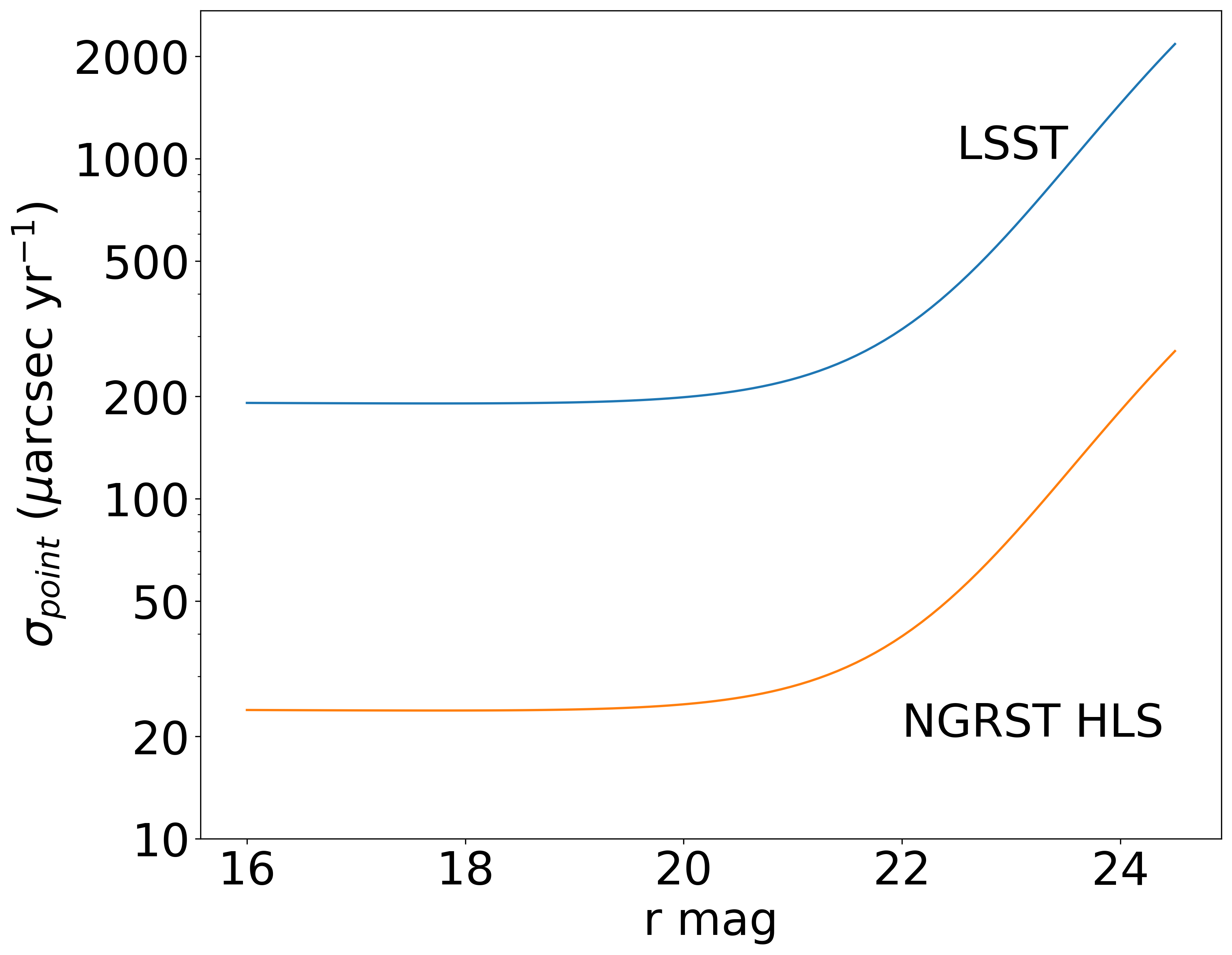
Figure 1: Astrometric proper motion error for a point source as a function of object magnitude, for both LSST and NGRST HLS. We show the fits used when generating the mock catalogues (Equation 9).

3.5.1 LSST astrometric errors

For the LSST, we take the form of the astrometric error $\sigma_{\rm point}(m)$ for a point source as a function of magnitude from Ivezić et al. (2012), where the relevant quantity is the proper motion error, rather than the parallax error. We use the following fitting function, accurate to within $2\%$:

$$\log{(\sigma_{\rm point})}=\log{(\sigma_{\rm bright})}+\frac{1}{2}(1+\tanh{(0.522(m-22.30))})\\ \times(0.172m-3.80-\log{(\sigma_{\rm bright})},$$ (9)

where $m$ is the apparent $r$ magnitude, and $\sigma_{\rm point}$ is in $\mu$arcsec yr^-1. Here $\sigma_{\rm bright}$ is the constant proper motion error expected at bright magnitudes. We plot $\sigma_{\rm point}(m)$ from this function in Figure 1, where we can see that it is expected to be approximately constant until $m\sim 20$, before increasing, reaching a maximum of $>2$ milliarcsec at the limiting magnitude of the survey. The constant error at bright magnitudes quoted by Ivezić et al. (2012) is $\sigma_{\rm bright}=\sigma_{\rm point}(m<20)=130$ $\mu$arcsec yr^-1, but in Figure 1 we have used a different value, to match the LSST Science Requirements, as follows.

In the LSST Science Requirements document, the design requirement for astrometric accuracy is relative astrometric precision for a single image of 10 mas (per coordinate). This translates to a a proper motion accuracy of $\sigma_{\rm bright}=200$ $\mu$arcsec yr^-1. The stretch goal is half of this value. When using mock catalogues (below), we treat $\sigma_{\rm bright}$ as a parameter to be varied, using values covering a range from 1 $\mu$arcsec$yr^{-1}$ to 3000 $\mu$arcsec$yr^{-1}$, with a fiducial value of 200 $\mu$arcsec$yr^{-1}$ (which is the value shown in Figure 1.

In the LSST Science Requirements, the relative rms astrometric error between two sources is dependent on the separation $D$ between them. The requirement above is valid for $D=20$ arcmin, and degrades by 50% if the relative separation is instead $20<D<200$ arcmin. In our case we are only interested in the proper motions of a tiny minority of galaxy sources, those within $z<0.06$. Each of these nearby galaxies will have its proper motion measured with respect to a frame consisting of many other more distant galaxies (and some quasars). For example, we expect that each of the $z<0.06$ galaxies will have on average $3\times 10^{5}$ LSST neighbour galaxies within 20 arcmin (assuming $2\times 10^{10}$ LSST galaxies in total). The astrometric error on the frame comprising these galaxies will be suppressed by a large $1/\sqrt{N}$ factor. The frame is therefore fixed by these distant galaxies, and so to a very good approximation the only relevant astrometric error for each of the low redshift galaxies is that in Equation 5. In the mock catalogues, we therefore add the astrometric(proper motion) error to each galaxy, with a direction chosen at random and a magnitude drawn from a Normal distribution with standard deviation $\sigma_{\rm astro}$.

3.5.2 NGRST astrometric errors

As a space based telescope, NGRST will continue the astrometric tradition of the Hipparcos and Gaia satellites. Compared to those instruments, it will have a much larger aperture, enabling observations of fainter stars. Crucially for this project, it is a multipurpose observing instrument, and will make images of the sky in four near infrared bands with high resolution. It is these images that we hope can be used to measure the proper motions of extended objects. Gaia and Hipparcos were limited to astrometry of point source objects, although the bright regions of galaxies can be registered as point sources (and were used to set limits on the cosmic parallax by Paine et al. 2020 ).

An overview of the astrometric precision that will be possible with NGRST and a study of the topics which can be addressed is given by Sanderson et al. (2017). These include measurements of the motions of stars in the distant Milky Way halo, constraints on dark matter from time dependent quasar lensing, and detection and characterisation of exoplanets. Sanderson et al. (2017) also address the detection of proper motions of local group galaxies, extending the reach of HST and Gaia by looking at individual stars such as bright K giants. The use of more distant galaxies to measure proper motions, such as we propose, it much more speculative, and would have to rely on techniques for dealing with extended images which have not been applied in the context of astrometry (see e.g., Section 3.5 above ). Although the apparent proper motions caused by cosmic parallax are miniscule on an individual basis, the wide area coverage of the HLS will allow thousands of well resolved galaxies within $z=0.06$ to be used to make a statistical measurement. As with the LSST case, the relative proper motions of nearby galaxies with respect to a larger number of more distant objects within 20 arcmins or less will be the quantity to measure. It is to be hoped that the requirement for relative astrometry rather than an absolute astrometric solution over the whole HLS footprint will be more forgiving.

Sanderson et al. (2017) also carried out a comprehensive analysis of the various physical effects which will need to be dealt with to achieve high precision astrometry. These include geometric distortion, pixel level (e.g., quantum efficiency) effects, colour dependence, and readout hysteresis. How best to schedule observations to maximise the astrometric value of various surveys (for example, how to organise the visits to the HLS fields over the 5 year nominal lifetime of NGRST) is also addressed. These issues will also be relevant for the extended object photometry that we are interested in here, and indeed there are likely to be additional concerns. As for the case of LSST, we do not address them here, but instead for the purposes of our simplified calculations assume that the point source proper motion precision can be applied to resolved elements of individual galaxies. Sanderson et al. (2017) list the approximate astrometric performance of the NGRST Wide-Field Imager, and for relative proper motions derived from the High-Latitude Survey, rms errors of 25 $\mu$ arcsec yr^-1 are expected for sources well above the magnitude limit. To set the proper motion error as a function of magnitude in our mock surveys, we set $\sigma_{\rm bright}=25\mu$ arcsec yr^-1 in Equation 9. We therefore use the same fitting function as for LSST, but with a smaller value for this parameter. The expected behaviour of the curve at faint magnitudes has not been estimated for NGRST, but the magnitude limit of the HLS is similar to LSST, and so with the advantages of space-based observations we feel that it is relatively conservative to assume the same form given by Equation 9 for NGRST.

3.6 Photometric redshifts

To constrain the redshift-distance relation, we need a parallax measurement that is a function of redshift. Unfortunately measuring spectroscopic redshifts for all galaxies observed by the LSST is unlikely to be possible in anywhere near the lifetime of the survey (we address the NGRST case below). In tests, we have explored the use of photometric redshifts exclusively, but have found that for the nearby galaxies ($z<0.06$) relevant for our present study, the error in the inferred distance is too large to allow the use of a velocity flow model correction (which is essential, see below). We therefore envisage the use of a subsample of galaxies with spectroscopic redshifts (to bin the parallax measurement vs. redshift). The rest of the galaxies with photometric redshifts will be used to define a distant frame which is at rest (as described above).

For photometric redshifts therefore, we only require that they be precise enough to differentiate between the nearby galaxies in our spectroscopic sample and those in the distant sample. Photometric redshifts will themselves be useful for targeting of the spectroscopic sample, in order to apply a volume limit. Predictions for and simulated tests of methods for the measurement of photometric redshifts for LSST galaxies have been made by Graham et al. (2018). The precision achieved in tests of the situation after 10 years of observations (over the redshift range $z=0.3-3.0$) is $\sigma_{\rm z}/(1+z)=0.0165\pm 0.001$, with a fraction of outliers equal to $0.04$.

Although the NGRST wide field camera operates in four photometric bands in the infrared, it will not be necessary to derive photometric redshifts from them, due to the grism observations which will also be available. The grism Spergel et al. (2013) will have $R=700$, which may be sufficient to achieve the redshift accuracy needed for the project, or else spectroscopic redshifts for the galaxy sample required could be obtained from another source.

3.7 Spectroscopic redshifts

Because we will be binning the measured cosmic parallax as a function of redshift from the observer, it is necessary to have an observed redshift associated with the galaxies in the mock surveys. We use the low $z$ approximation, $z=H_{0}d/c+v_{\rm pec}/c$ to assign redshifts $z$ to each galaxy, where $v_{\rm pec}$ is the peculiar velocity component along the line of sight to the observer. We then assume that spectroscopic redshifts are available (for both LSST and NGRST HLS) for a small fraction of observed galaxies above a certain apparent magnitude limit. This fraction is varied in Section 5.3, but we use $r<18$ to define it in the fiducial case. We add also a measurement error taken from a Normal distribution with $\sigma=100$ $\,{\rm km}\,{\rm s}^{-1}$ to each galaxy’s redshift.

In the case of the LSST, this accuracy could be achieved from a separate redshift survey with comparable redshift precision to e.g., the SDSS (Blanton et al., 2005), but in the southern hemisphere. For NGRST HLS, the sky area and therefore number of galaxies with $r<18$ is much smaller, and so it should not be difficult to obtain redshifts for them even if the NGRST grism itself is unsuitable. As we see will see in Section 5.3, the number of redshifts required below this magnitude limit for NGRST would be about $40,000$.

3.8 Peculiar velocities

The three-dimensional rms peculiar velocity of galaxies in the simulation is $\sigma_{V3D}=550\,{\rm km}\,{\rm s}^{-1}$. This will lead to both shifts in the Hubble redshift diagram as well as a peculiar velocity error component (which could be deemed an actual proper motion) to the measured parallax. On a galaxy by galaxy basis, this proper motion component is relatively small. For example, a galaxy with redshift $z$ in our mock survey will have an rms proper motion due to peculiar velocities of $0.8\frac{0.05}{z}\mu$arcsec yr^-1. This would seem to be much smaller than the astrometric error $\sigma_{\rm astro}$ for all except extremely nearby galaxies (for example galaxies within 1$h^{-1}{\rm Mpc}$ will have rms proper motions of $\sim 100\mu$arcsec yr^-1). Unfortunately, the large scale velocity field has a high degree of coherence (e.g., Gorski et al., 1989), and as a result these proper motion errors do not decrease by simple $\sqrt{N}$ averaging. Indeed, as we shall see below, lack of knowledge of the peculiar velocity field over the survey volume will be the main limiting factor for the precision of the cosmic parallax measurement.

The effect of peculiar velocities has of course been noted by many authors (e.g., Howlett & Davis 2020; Mukherjee et al. 2019; Nicolaou et al. 2019 in the context of distorting the redshift-distance relation for other probes, such as standard sirens. In these studies, corrections have been applied using models for the peculiar velocity flow field derived from the gravity field of large-scale structure (such as Springob et al. 2014). Paine et al. (2020) have extended this analysis to cosmic parallax, where the predicted angular proper motion of galaxies was examined based on the Cosmicflows-3 galaxy peculiar velocity catalogue (Tully et al. 2016). In our case, we will examine the effect of peculiar velocities in our simulated mock surveys. We will study cases where the velocity field is not corrected, and also where predictions for or measurements of the peculiar velocities are used to correct them to a certain degree of accuracy.

In our mock catalogues we therefore add the component of the peculiar velocities of each galaxy along the observer’s line of sight to the measured redshift. We also add the components of the proper motion due to the peculiar velocity to the measured proper motion.

4 Determination of the Hubble constant: method

4.1 Measurement of galaxy parallax

For a mock (or real survey), we have information on the measured total astrometric proper motion of each galaxy, which includes cosmic parallax, measurement errors and peculiar velocity component, as well as the spectroscopic redshift of each galaxy, again including redshift errors and peculiar velocities. To analyze each mock and measure the Hubble constant from it, we first divide the galaxies into bins of measured spectroscopic redshift, and for each bin compute the weighted mean of the proper motion component in the direction expected for cosmic parallax. The measured parallax is then

$$\pi(z)=\frac{1}{\sum_{i=1}^{N(z)}w_{i}}\sum^{N(z)}_{i=1}w_{i}\,\sqrt{1-(\hat{n}\cdot\vec{\mu_{i}})^{2}},$$ (10)

where the sum $i$ is over the $N(z)$ galaxies, in the bin centered on redshift $z$. Here $\hat{n}$ is a unit vector on the surface of the celestial sphere pointing towards the apex of the CMB motion, and $\vec{\mu_{i}}$ is a vector representing the measured astrometric proper motion of galaxy $i$. The inverse variance weighting used is

$$w_{i}=\frac{1}{\sigma^{2}_{\rm pm}+\sigma^{2}_{\rm astro,i}},$$ (11)

where $\sigma^{2}_{\rm astro,i}$ is the square of the rms astrometric measurement error for galaxy $i$ (from Equation 5). Here, $\sigma^{2}_{\rm pm}$ is the square of the rms proper motion for galaxies at redshift $z$, computed from $\sigma_{\rm pm}=\sigma_{v}/r(z)$ where $\sigma_{v}$ is the rms peculiar velocity, and $r(z)$ is the parallax distance to redshift $z$, from Equation 2. As described in Section 3.5, in our fiducial case, we make use of the separate elements of each resolved galaxy to determine $\sigma^{2}_{\rm astro,i}$ for the galaxy.

We compute the error bars on $\pi(z)$ from the standard deviation of the values from all 54 mock catalogues, and also compute the covariance matrix between redshift bins. In order to determine the value of the Hubble constant, we compare the measured $\pi(z)$ to a theoretical curve and fit an amplitude parameter. The theoretical curve is derived from Equation 4, but smoothed by peculiar velocities and redshift errors. These would have a substantial impact if only photometric redshifts were used, but in our case, as spectroscopic redshifts are employed to bin galaxies. so the difference between Equation 4 and the smoothed version is small, as we see below.

4.2 Predicted parallax

In order to estimate the Hubble constant, it is necessary to compare the results of a cosmic parallax measurement (from Equation 10) with a prediction. The predicted parallax for a set of objects with no peculiar velocities, and redshifts which fall exactly at the centers of the redshift bins used in the measurement, and which are all at the same angle with respect to the apex of the CMB motion can be computed using Equation 4. At the level of accuracy required to make competitive estimates of the Hubble constant however, the non uniformity in redshift and angle of the sample of galaxies used will result in any binned estimate of redshift, angle, and parallax having significant Poisson errors. We therefore include information which will be available from observations for the individual galaxies when making the prediction. This information is their angular positions, their spectroscopic redshift, and when relevant, estimates of their peculiar velocities from a flow model (see Section 4.4). The predicted parallax for an assumed value of $H_{0}$ is therefore:

$$\pi_{\rm p}(z)=\frac{1}{\sum_{i=1}^{N_{p}(z)}w_{i}}\sum^{N_{p}(z)}_{i=1}w_{i}\,\pi(H_{0},z_{p,i})\left|\sin{\theta_{i}}\right|$$ (12)

where the sum $i$ is over the $N_{p}(z)$ galaxies, in the bin centered on redshift $z$. Here $\theta_{i}$ is the angle between the position of galaxy $i$ and the apex due to the CMB motion. Equation 4 is used to compute $\pi(H_{0},z_{p,i})$, where $z_{p,i}$ is the spectroscopic redshift of galaxy $i$. If a flow field model (Section 4.4) is used, $z_{p,i}$ is instead the spectroscopic redshift minus the line of sight component of the flow field peculiar velocity. The weight $w_{i}$ is taken from Equation 11.

4.3 Use of spectroscopic redshifts

Because we are focusing on low redshift observations $z<0.06$, we find that the LSST photometric redshift accuracy $\sigma_{z}\sim 0.02$ (Graham, 2019) is too low to allow precise measurement of $\pi(z)$. This is not because of the smoothing effect of redshift errors on the $\pi(z)$ curve, but instead because the photometric redshifts do not allow the galaxy three dimensional positions to be estimated well enough to apply a peculiar velocity correction (see below). In order to do this, we estimate that a sample of spectroscopic redshifts (for both LSST and NGRST HLS will need to be collected, for the brightest galaxies within a photometric redshift limit .

For our fiducial analysis of mocks, we assume that spectroscopic redshifts will be available for galaxies with $r<18$. This is similar to the SDSS main galaxy sample, which had Petrosian $r<17.77$. The use of photometric redshifts to preselect low redshift targets will further reduce the total number of redshift measurements needed. At present the largest planned samples of galaxies with spectrocopic redshifts are in the northern hemisphere (DESI, Schlegel et al. 2015, and WEAVE, Bonifacio et al. 2016 ), but the redshift requirement for the cosmic parallax measurement is modest compared to these surveys. For example, we find that in our mock surveys that if all galaxies with photometric redshift $z<0.06$ and $r<18$ are targeted, the sample per survey is about 400,000 galaxies for LSST and 40,000 for the HLS. In our analysis we will vary the magnitude limit, and find that competitive estimates of $H_{0}$ could be possible even with a magnitude limit as low as $r<14$ for spectroscopic redshifts, which would be only 12,000 galaxies on average from an LSST survey.

The photometric redshifts of all galaxies are still useful for the parallax measurement. Even though we only directly use galaxies with spectroscopic redshifts in our binned $\pi(z)$ determination, the parallax measurements for those galaxies will have been obtained as differential measurements, where the angular displacements are obtained with respect to a frame defined by much more numerous distant galaxies that are close on the sky. That they are more distant will be ensured through the use of the photometric redshifts available for all galaxies brighter than $r=27.8$ for LSST, and $Y=25.8$ for NGRST HLS.

4.4 Accounting for peculiar velocities

Peculiar velocities will distort the parallax distance-redshift relation. Because we concern ourselves here with nearby galaxies, with recession velocities $cz<18,000\,{\rm km}\,{\rm s}^{-1}$, the coherent flows of galaxies due to gravitational instability will be a more important factor than they are for e.g., cosmology with Type IA supernovae (Davis et al., 2011). It is customary to correct galaxy redshift for the effects of peculiar velocities using a flow model when determining the nearby distance redshift relation (for example see the early work of e.g., Willick & Batra 2001 for cepheids, or more recently Mukherjee et al. 2019). Flow models can be constructed using the predicted gravitational potential computed from the galaxy density field (using a bias model) and linear theory or other models to relate the peculiar velocities to the acceleration. Examples of such flow models are Branchini et al. (1999) and Springob et al. (2014).

The accuracy of such flow models can be tested to some extent using N-body simulations. For example, the PIZA algorithm of Croft & Gaztanaga (1997) can recover the velocity field smoothed on scales of 5 $h^{-1}{\rm Mpc}$ with an rms error of $37\,{\rm km}\,{\rm s}^{-1}$. In general, the velocity field in flow models is predicted on a grid, which can be interpolated to the positions of galaxies, leading to a further dispersion of peculiar velocities between galaxies and the interpolated grid. In the present work, we do not apply a particular flow field reconstruction method to our mock catalogues, but instead use the actual smoothed velocity field of galaxies as a correction, and add an rms dispersion (a parameter to be varied) to model the effects of non-linearities and galaxy bias. We leave the implementation and use of an actual flow field reconstruction method (such as Colombi et al. 2007, or Yu & Zhu 2019) and tests on simulations to future work.

Our procedure is as follows. We assign the redshift-space positions of the simulated galaxies in the mock surveys to a three dimensional grid of cell size $5h^{-1}{\rm Mpc}$ using a nearest grid cell assignment scheme. We also assign the peculiar velocities of galaxies to the same grid, weighting by number, to produce a flow field grid. We smooth the grid with a Gaussian filter with $\sigma=5h^{-1}{\rm Mpc}$. We use this smoothed flow field to correct the galaxy angular proper motions in the mock survey, by subtracting the flow velocity for the cell containing the galaxy (again in redshift space, including redshift errors), and adding a random dispersion velocity component. Our fiducial random velocity dispersion is $100\,{\rm km}\,{\rm s}^{-1}$ (for comparison, Nicolaou et al. 2019 find a residual velocity error in a galaxy of $36\,{\rm km}\,{\rm s}^{-1}$, and Abbott et al. 2017 find $69\,{\rm km}\,{\rm s}^{-1}$ ). We also use the flow field to correct the redshift space positions of galaxies to real space, by subtracting the line of sight component of flow model velocity from the observed redshift (see e.g., Gramann et al. 1994, Croft & Gaztanaga 1997, and Wang et al. 2020 for other methods).

When constructing a flow field prediction, the relationship between galaxies and mass needs to be specified, as the mass governs the gravitational accelerations. This is an area where the galaxy angular motion information from Rubin Observatory and NGRST will be very useful, and the astrometry be used to validate and calibrate the flow field model. For example, the linear bias (the constant of proportionality relating the galaxy and mass overdensities) could be left as a free parameter. Varying this parameter would change the flow field model used as a correction. The best fit of $H_{0}$ and the bias parameter together could be obtained by comparing to the galaxy angular motion measurements. Measuring galaxy transverse proper motions statistically has been discussed by Darling et al. (2018), Hall (2019) and Paine et al. (2020). The use of astrometry in this way could make the flow field model and distance estimate of $H_{0}$ internally consistent, and eliminate any need to consider other sources of distance information.

5 Results

We have carried out the analysis described above on our mock LSST and NGRST HLS surveys. In order to study how the results depend on survey analysis parameters, we have varied them from their fiducial values. These are first described below.

parameter	description	fiducial value	fiducial value
		for LSST	for NGRST HLS
$\sigma_{\rm bright}$	$rms$ proper motion error for bright objects	200 $\mu$arcsec/yr	25 $\mu$arcsec/yr
$r$ mag	limiting galaxy $r$ magnitude	18	18
$f_{\rm res\ elements}$	fraction of resolved elements used independently	0.5	0.5

Table 1: Fiducial parameter values used in mock catalogues.

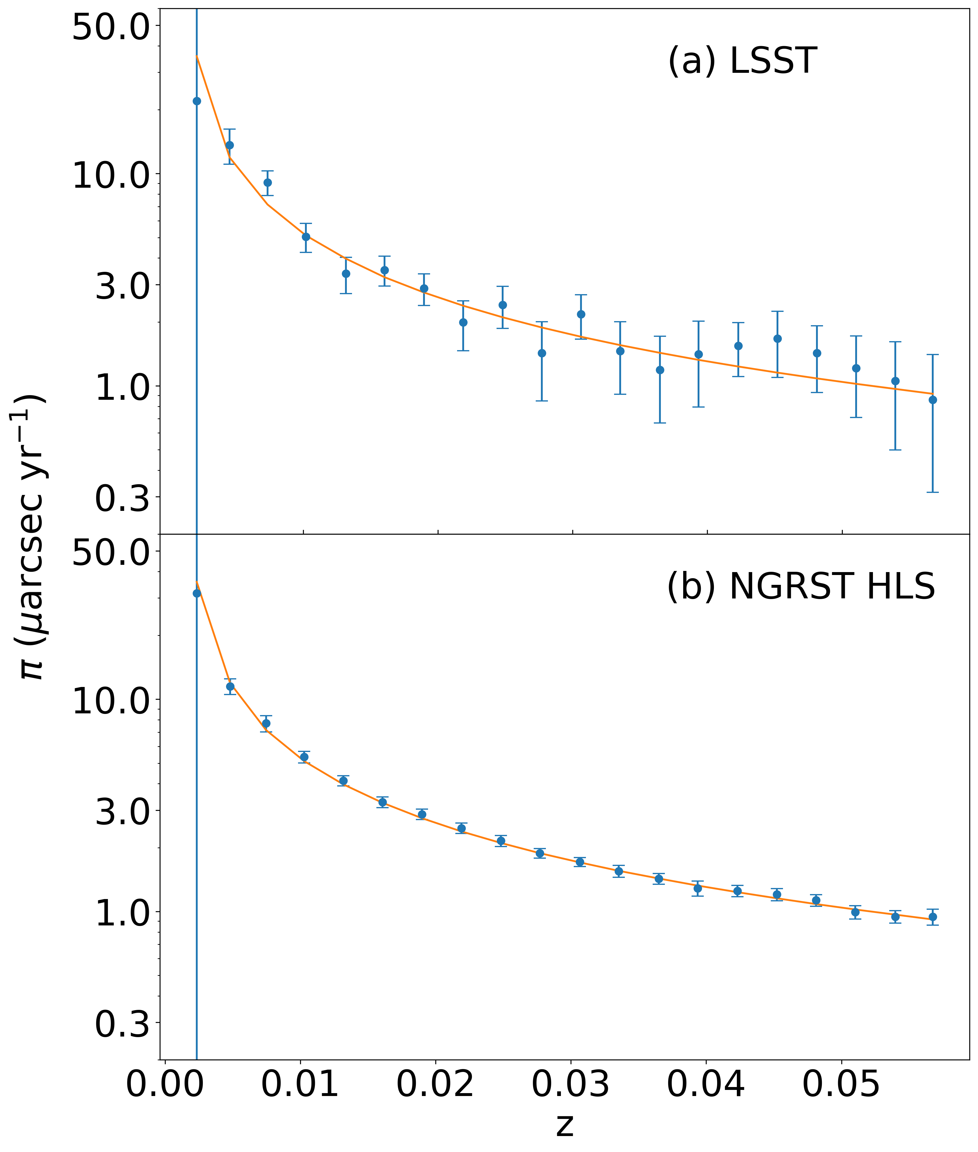
Figure 2: Secular parallax vs. redshift. Points with error bars show results from (a) an example mock LSST, and (b) a mock NGRST HLS, using galaxies with $r<18$ (with spectroscopic redshifts). The smooth curve shows the theoretical prediction made using Equation 12 and with the correct value of $H_{0}$.

5.1 Fiducial analysis

In our fiducial analysis, we assume that the peculiar velocities leading to angular proper motions (and redshift distortions) can be corrected with the aid of a flow model (Section 4.4). We investigate what happens when this is not the case in Section 5.4 below. Apart from this, we also vary the following three parameters The first is $\sigma_{\rm bright}$, the rms proper motion error for bright objects (in Equation 9), with the fiducial value for LSST being that given in the LSST science requirements, 200 $\mu$ arcsec yr ^-1, and the value for NGRST HLS, 25 $\mu$ arcsec yr ^-1 taken from Sanderson et al. (2017). The second parameter is $r$ mag, the limiting $r$ magnitude of galaxies used in the sample (and which have spectroscopic redshifts). We choose $r$ mag=18 as the fiducial value. The third parameter is $f_{\rm res\,elements}$, and relates the number of resolved elements of a bright galaxy that are used separately to compute the astrometric motions to the total number. We therefore modify Equation 5 to read

$$\sigma_{\rm astro}=\sigma_{\rm point}(m_{e})/(f_{\rm res\,elements}\sqrt{N_{\rm elem}}),$$ (13)

We assume that information from a significant fraction of the resolution elements would be used, using $f_{\rm res\,elements}=0.5$ as our fiducial value. The true value should be computed with tests on galaxy images (as discussed in Section 3.5). We explore the effect of widely varying values of $f_{\rm res\,elements}$ in Section 5.4.

The three parameters and their fiducial values are summarised in Table 1. With these values, we compute the measured parallax as a function of redshift following the methodology in Section 4.1. We use 20 bins equally spaced in redshift between $z=0$ and $z=0.0583$ (a distance of 175 $h^{-1}{\rm Mpc}$). We also compute the predicted $\pi(z)$ curve for the correct $H_{0}$ value, in a manner that uses information that would be available from observations (Equation 12).

We plot the results for a single randomly chosen mock survey in Figure 2. To allow easier comparison between surveys in the plot, we scale both the LSST and NGRST HLS predictions and measured datapoints (and error bars) upwards by 1 divided by the mean of $\sin{\beta}$ over the respective survey footprint. Here $\beta$ is the angle between a galaxy and the CMB apex (Equation 4). From Figure 2 we can see the the measurements scatter about the predicted line, and that there is measurable signal over the entire redshift range plotted, even for LSST, which has the largest error bars. Even at $z\sim 0.06$, the signal to noise per bin is $\sim 2$ for LSST and $\sim 10$ for NGRST HLS, indicating that it could be productive to extend the measurements to higher redshifts. Because of the relatively small size of our simulated catalogues we leave this to future work.

As stated above, we compute the elements of the covariance matrix of the points in Figure 2 from the scatter between results for the 54 mock catalogues. Then use this covariance matrix to compute the best fitting value of an overall amplitude parameter scaling the value of $H_{0}$. We use the Python routine scipy.optimize.curve$\_$fit to compute the fit amplitude, using least squares minimization. This yields a best fitting value of $H_{0}/H_{0,true}$ for each catalogue, as well as a measurement error. A histogram of $H_{0}/H_{0,true}$ for our fiducial analysis is shown in Figure 3, where we can see that the values lie between $H_{0}/H_{0,true}=0.95$ and $1.06$ for LSST, being relatively symmetrical, and $0.98$ and $1.02$ for NGRST HLS. The mean (median) $H_{0}/H_{0,true}$ values are 1.008 (1.008) for LSST, and 0.998 (0.997) for NGRST.

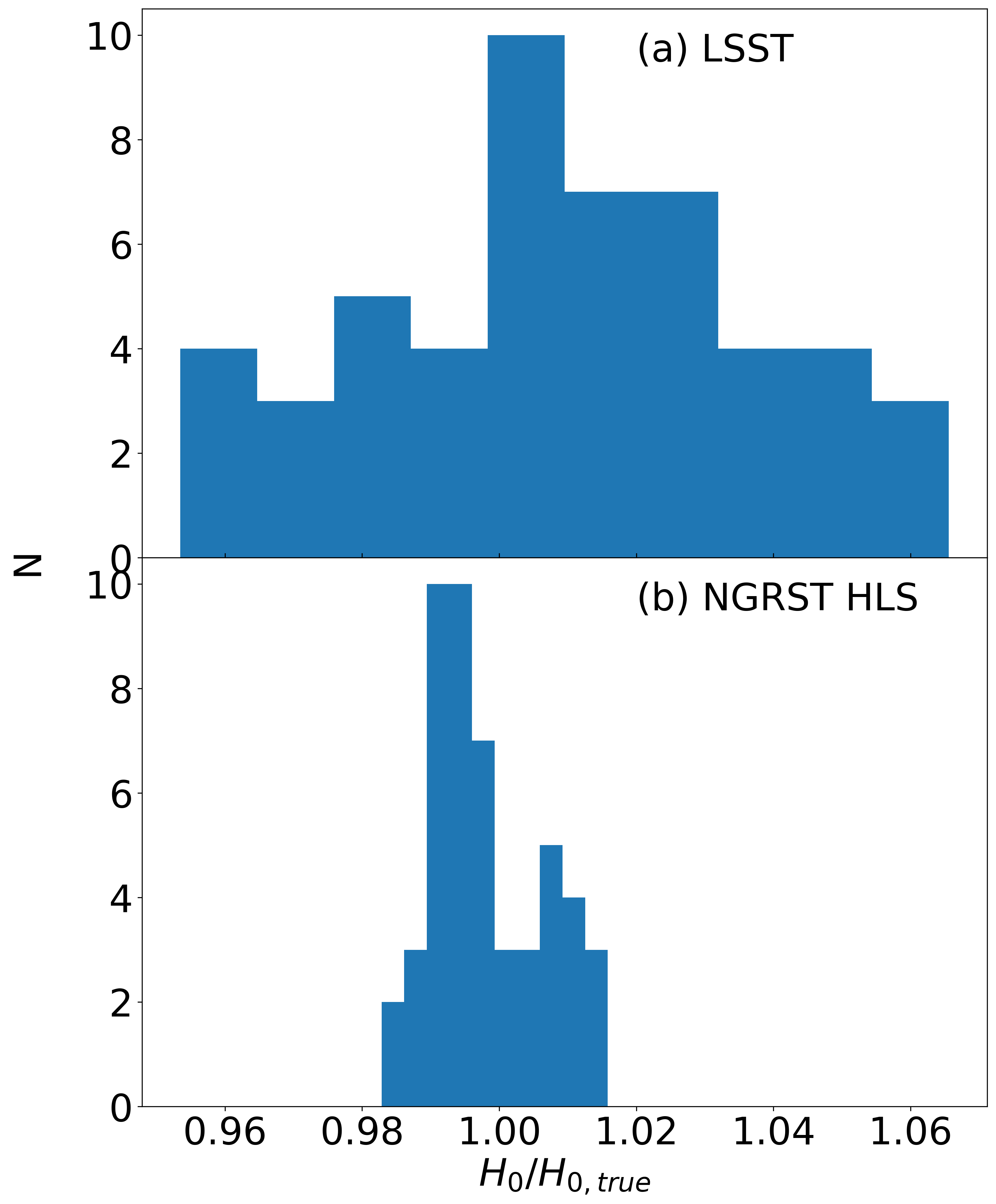
Figure 3: Histograms of $H_{0}$ measurements for (a) mock LSST surveys and (b) mock NGRST HLS surveys. We show results for the fiducial case (Section 5.1).

We compute an estimate of the mean fractional error on $H_{0}$ from the standard deviation of the results for all mock surveys plotted in Figure 3, finding a value of 2.8% for LSST and 0.8% for NGRST HLS (these values are for our fiducial analysis and parameter choices). Error estimates for each mock survey are also available individually, and a histogram of the one sigma error bar sizes is plotted in Figure 4. The mean of these fractional errors is also 2.8%, with values ranging from 1.6% to 4.5% (LSST) and mean 0.8% with range 0.5% to 1.3% (NGRST). The $\pm 1\sigma$ spread of the error estimates is $\pm 0.5$ % (LSST) and $\pm 0.15\%$ (NGRST).

Using the error bars on each measurement of $H_{0}/H_{0,true}$ allows us to see if the measurement is unbiased. Because we have 54 mock surveys, the statistical error on the mean $H_{0}/H_{0,true}$ value from all of them is 2.8%$/\sqrt{54}=$0.38% for LSST. Our mean $H_{0}/H_{0,true}$ ($1.009$, mentioned above) is therefore $(1.008-1.0)/0.0038=2,1\sigma$ from the expected value of $1.0$, and therefore for LSST the method is unbiased at the $\sim 2\sigma$ (based on all 54 surveys). Of course an actual observational measurement would be made from a single survey, and this bias would correspond to $(2.1/\sqrt{54})=0.3$ times the statistical error bar, which is subdominant. This small bias is likely arises because the observed redshifts of the galaxies used to make the predictions in Equation 12 are not the true Hubble redshifts which govern the actual galaxy parallax (Equation 4). For NGRST HLS, the equivalent calculation also reveals a 2$\sigma$ bias for the mean of all 54 surveys and $0.3\sigma$ for an individual survey.

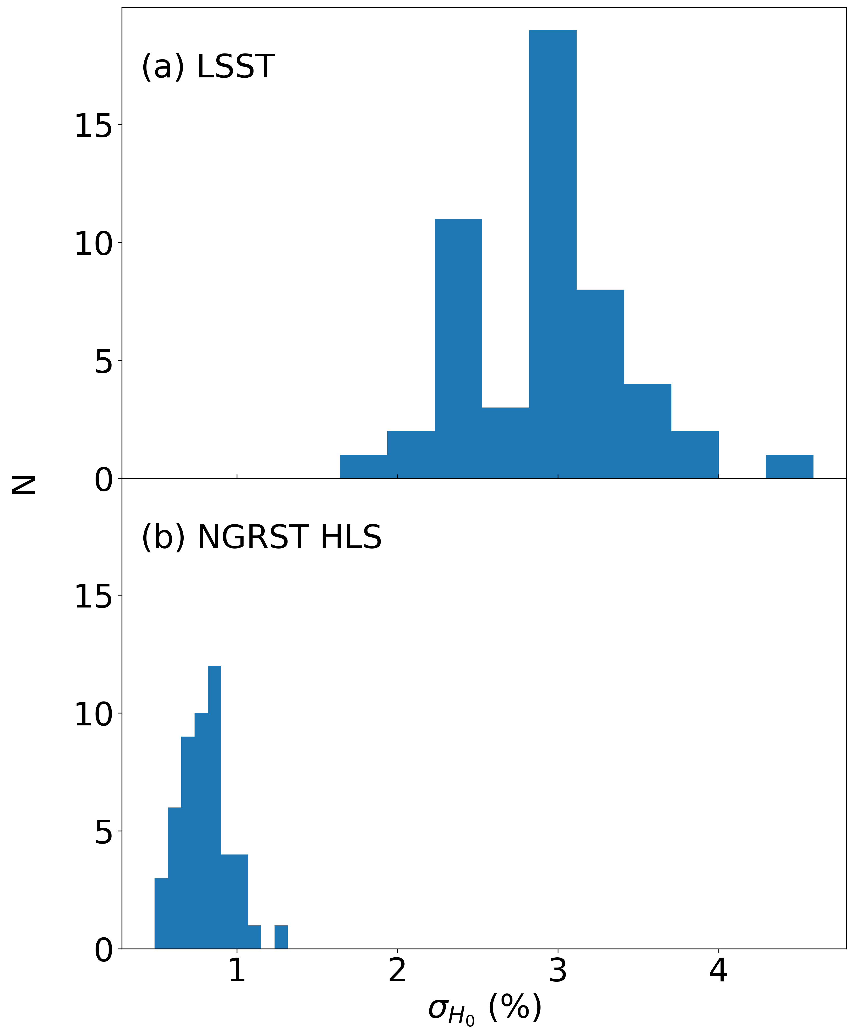
Figure 4: Histograms of $H_{0}$ fractional measurement errors for (a) mock LSST surveys and (b) mock NGRST HLS surveys. We show results for the fiducial case (Section 5.1).

5.2 Impact of astrometric errors

In our fiducial analysis we used the astrometric error as a function of magnitude from the predictions shown in Figure1 for LSST and NGRST HLS. Depending on many factors related to the functioning of the telescopes and the surveys, the astrometric precision achieved could be better or worse. We parameterise the overall precision using the $\sigma_{\rm bright}$ limiting astrometric error for bright objects, as explained in Section 5.1. We have varied the parameter $\sigma_{\rm bright}$ between 1 and 3000 $\mu$ arcsec yr ^-1, making new mock surveys for both LSST and NGRST HLS each time, and computing the fractional error on $H_{0}$ measurements, $\sigma_{H_{0}}$. The results are shown in Figure 5, where the rest of the analysis is kept as in the fiducial case (orange line). The $\sigma_{H_{0}}$ values span 0.15% to 100% (LSST) and 0.4% to 25% (NGRST) over the range of $\sigma_{\rm bright}$ values tried.

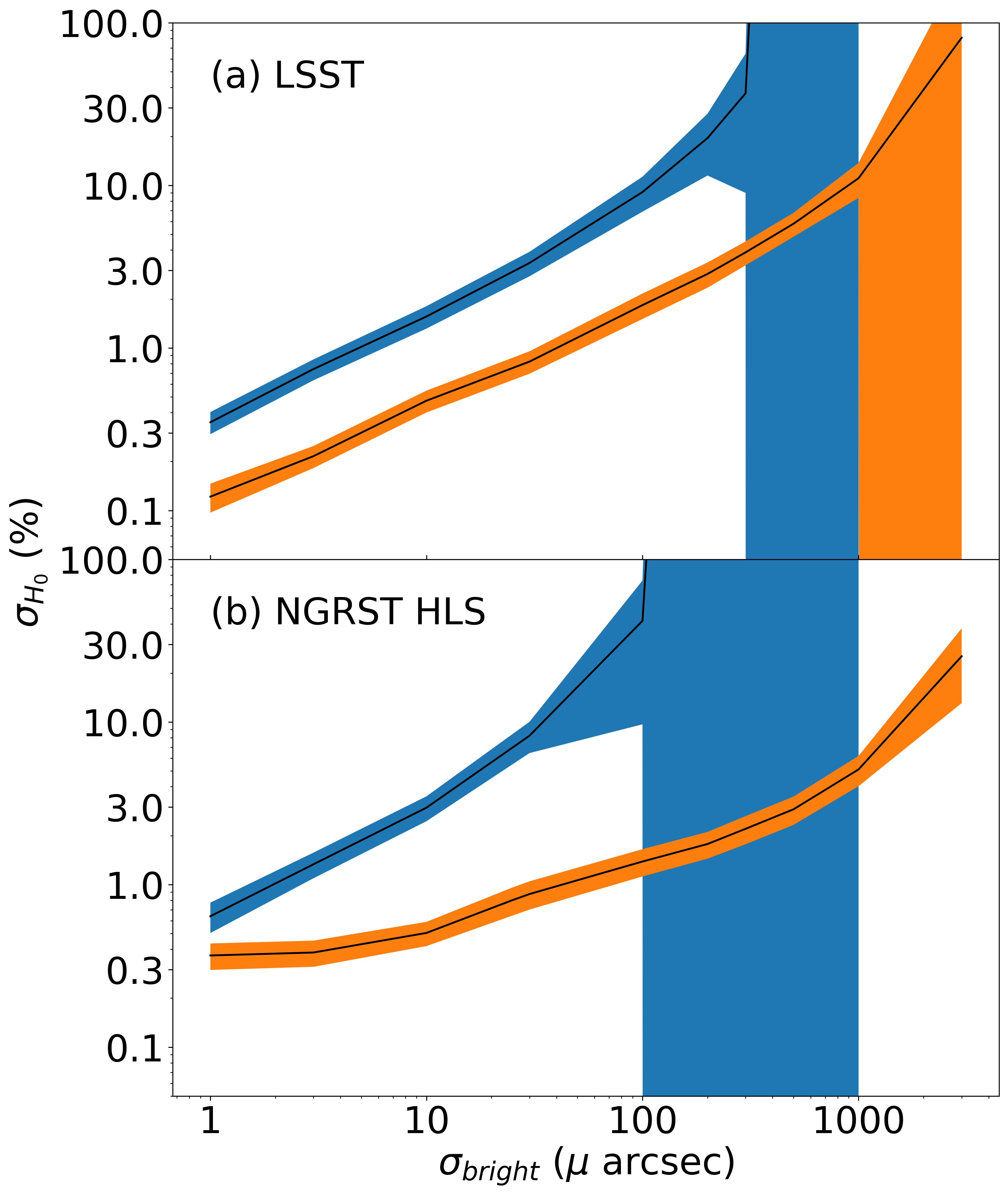
Figure 5: The rms percentage error on $H_{0}$ measurements as a function of the astrometric error for bright sources, $\sigma_{\rm bright}$. The results shown in orange are for the case where the rest of the fiducial analysis is kept the same, and the results in blue restrict the number of astrometric measurements to one per galaxy (rather than making use of separate resolution elements). The envelope around each line illustrates the standard deviation of the $\sigma_{H_{0}}$ values for the mock surveys. The top panel, (a) is for mock LSSTs, and the bottom panel, (b) is for mock NGRST HLSs

Our fiducial analysis includes the statistical reduction of astrometric errors caused by the consideration of the separate resolved elements of bright galaxies. It is interesting to relax this assumption, in order to see how much worse the distance estimates would be. We do this by degrees in Section 5.4 below, but in the present case, we have also plotted in Figure 5 (blue) lines showing results where each galaxy is only used to compute one secular parallax measurement, irrespective of size or apparent magnitude. We can see that in this case the errors on $H_{0}$ are significantly larger, and increase rapidly. For the LSST. when $\sigma_{\rm bright}=10$ $\mu$ arcsec yr ^-1, $\sigma_{H_{0}}=1.6$%, increasing to 37% for $\sigma_{\rm bright}=300$ $\mu$ arcsec yr. For NGRST, the increase in $\sigma_{H_{0}}$ with $\sigma_{\rm bright}$ is even more rapid. This illustrates that it will be critical to develop techniques to make full use of the resolved elements of large galaxies, and without this $H_{0}$ measurements are unlikely to be feasible for LSST and likely be uncompetitive for NGRST HLS. We should bear in mind that the samples of galaxies used in Figure 5 are those brighter than our fiducial apparent magnitude limit of $r=18$, and are assumed to have spectroscopic redshifts. Therefore the blue lines make use of many fewer galaxies than will be observed by the LSST or NGRST HLS and will have photometric (or grism) redshifts. Although the number increase for a photometric sample would decrease the statistical errors, we have found (Section 4.4 that spectroscopic redshifts are essential for correcting the effects of peculiar velocities, at least for the nearby sample of galaxies considered in this paper.

5.3 Apparent magnitude limits

We now explore the effect of limiting apparent magnitude on the sample of galaxies used. Our fiducial value is $r$ mag$=18$, and we assume that only galaxies brighter than this will have spectroscopic redshifts. Fainter galaxies will still be used to set the astrometric reference frame local to each bright galaxy (see Section 3.5). When we decrease the limit from $r<18$ to $r<16$, the mean number of galaxies in each mock LSST survey decreases from 390,000 to 78,000, but the error on $H_{0}$ only increases from $\sigma_{H_{0}}=2.7$ % to 2.9%. For NGRST the situation is similar. This is largely a consequence of the fact that the fainter galaxies which are being eliminated make a much smaller constribution than the bright galaxies which cover many resolution elements. The yellow curves in Figure 6 show these results, where we can see that the mean error on $H_{0}$ changes slowly with magnitude to even brighter magnitude limits, even down to $r=11$ for LSST. We stop plotting results below this because there are only 700 galaxies being used and some of the redshift bins for individual surveys start becoming empty because of Poisson fluctuations. The NGRST HLS result cuts off at $r=13$ and below, for the same reason (there are a similar number of galaxies per survey at this limiting magnitude). The shaded regions around the lines show the statistical $1\sigma$ error on the $\sigma_{H_{0}}$ values, computed from the scatter between results for the different mock surveys. Adding galaxies fainter than $r=18$ to the sample does not noticeably increase the precision of the $H_{0}$ measurement, which remains within the 1 $\sigma$ error on $\sigma_{H_{0}}$ for both LSST and NGRST HLS.

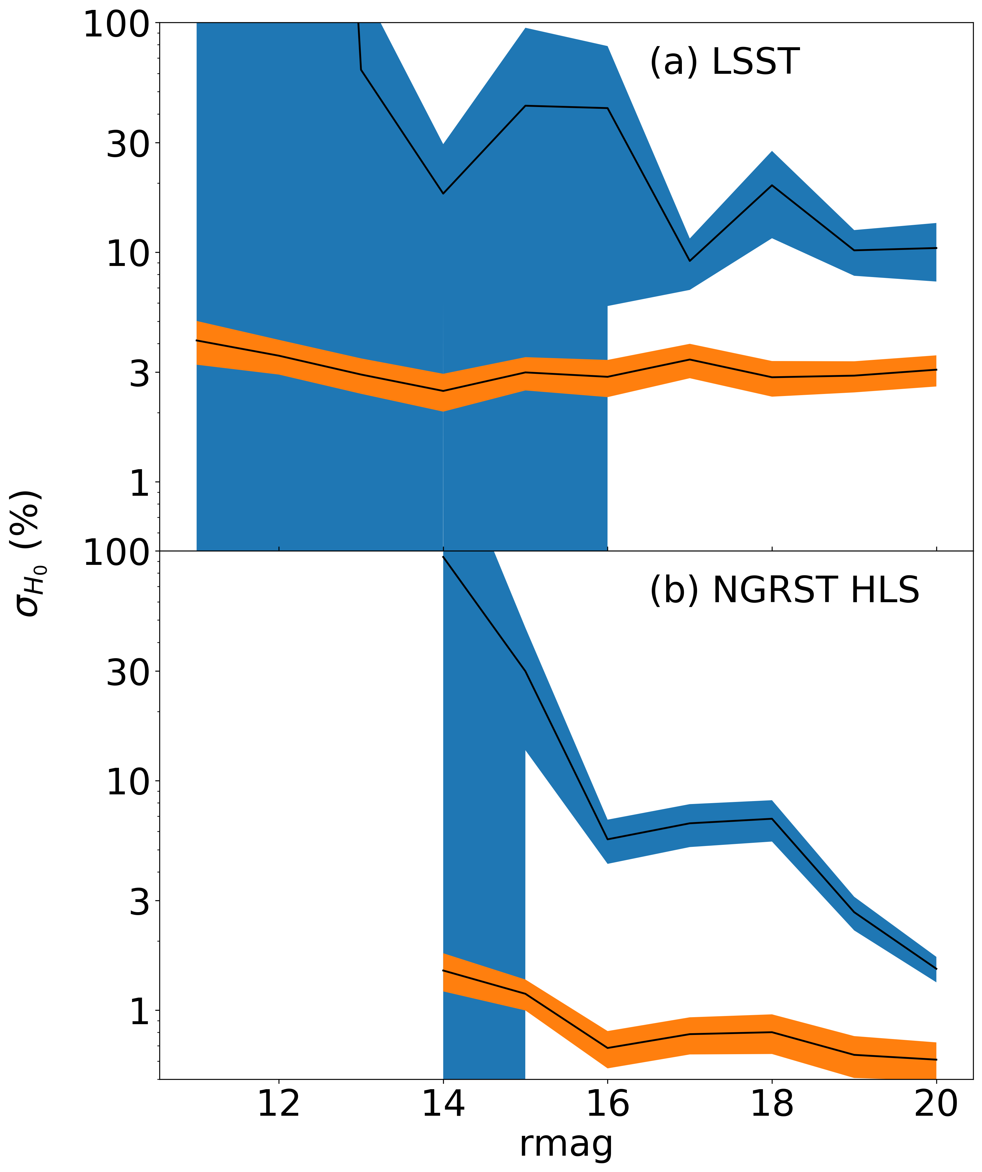
Figure 6: The rms percentage error on $H_{0}$ measurements as a function of magnitude limit for galaxies used. The results shown in orange are for the case where the rest of the fiducial analysis is kept the same, and the results in blue restrict the number of astrometric measurements to one per galaxy (rather than making use of separate resolution elements). The envelope around each line illustrates the standard deviation of the $\sigma_{H_{0}}$ values for the mock surveys. The top panel, (a) is for mock LSSTs, and the bottom panel, (b) is for mock NGRST HLSs.

As for Section 5.2, we have also computed a curves for analyses where the resolution elements of galaxies are not used independently. These are shown as a blue lines in each of the LSST and NGRST HLS panels. We can see that even extending the number of galaxies used by a large factor with a magnitude limit of $r=20$ (which results in 1.8 million galaxies on average per LSST mock) does not decrease the error on $H_{0}$ to below 10% for LSST, indicating that techniques to make use of separate resolved elements will be essential in this case for a competitive measurement. For NGRST, the situation is better, and although $\sigma_{H_{0}}=6.8\%$ for the fiducial $r=18$ magnitude limit, it does decrease to $\sigma_{H_{0}}=1.5\%$ for $r=20$. Of course in this case it will still be necessary to make one measurement for each galaxy, which are extended objects and so this will not be straightforward.

5.4 Impact of independent image elements and velocity reconstruction

How well one can use the individual resolved elements of galaxies to improve the astrometric measurement precision is an open question. Future work should test this with simulations and tests with observational data. In the meantime, we have varied the parameter $f_{\rm res\,elements}$ described in Section 5.1 to quantify the how the fraction of resolved elements that are used independently affects the overall measurement error on $H_{0}$. In Figure 7 we show the results of varying $f_{\rm res}{\rm elements}$ from 0.001 to 1.0. With our fiduc ial value, $f_{\rm res\,elements}=0.5$ we have the values of $\sigma_{H_{0}}=2.8$% (LSST) and $\sigma_{H_{0}}=0.8$% (NGRST HLS) quoted above. This decreases to $\sigma_{H_{0}}=2.6$% (LSST) and $\sigma_{H_{0}}=0.7$% (NGRST HLS) when $f_{\rm res\,elements}=1.0$. Although $\sigma_{H_{0}}$ increases as $f_{\rm res\,elements}$ decreases, even when $f_{\rm res}{\rm elements}=0.001$, $\sigma_{H_{0}}$ is significantly better than for the case when each galaxy is only used to make a single measurement (see Figure 6). We find that bright LSST galaxies with $r\sim 15$ at redshifts $z\sim 0.03$ (about halfway to the far mock boundary) typically contain $\sim 3000$ resolved elements. If this can be exploited, it is this which will give the astrometry measurements their power.

In the same figure, 7 we also show the effect of not including any peculiar velocity flow modeling, as grey curves. We can see that the peculiar velocities dominate the error on $H_{0}$, and even when using all elements of resolved galaxies, $f_{\rm res}{\rm elements}=1.0$, the value of $\sigma_{H_{0}}$ stays at about 20% for the LSST. For NGRST HLS, because the mock volumes are an order of magnitude smaller than for LSST, the effect of not correcting for peculiar velocities is much worse, with $\sigma_{H_{0}}$ being around 100%. All components of our fiducial modeling will therefore have to be applied and work well if the technique is to yield a competitive measurement (or even a detection in the case of NGRST).

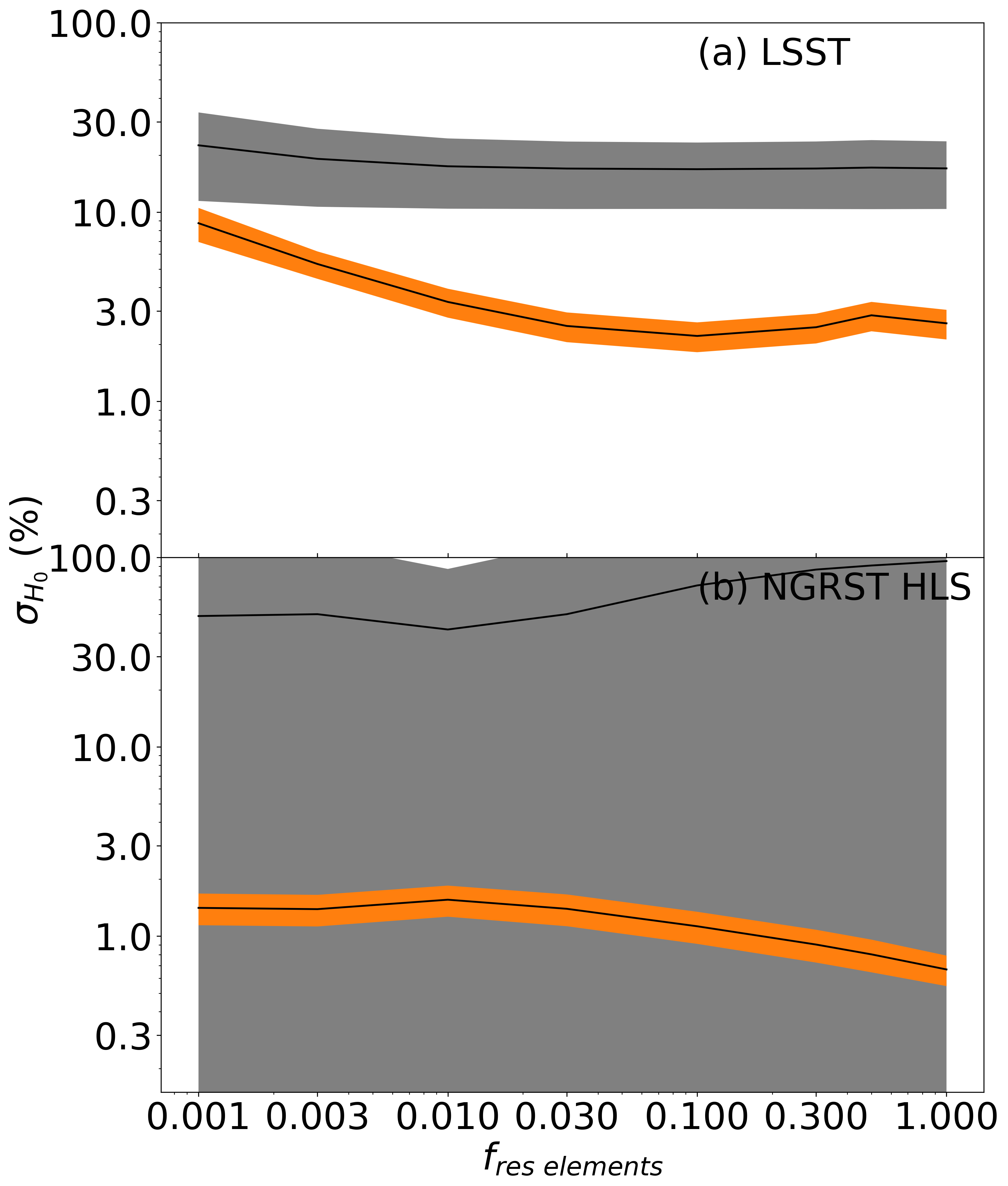
Figure 7: The rms percentage error on $H_{0}$ measurements as a function of the parameter $f_{\rm res\,elem}$ in Equation 13, which governs the fraction of resolution elements in each galaxy which are used to make independent astrometric measurements. The results shown in orange are for the case where the rest of the fiducial analysis is kept the same (including application of a velocity flow model to correct peculiar velocities). The results in gray are for an analysis with no peculiar velocity corrections. The envelope around each line illustrates the standard deviation of the $\sigma_{H_{0}}$ values for the mock surveys. The top panel, (a) is for mock LSSTs, and the bottom panel, (b) is for mock NGRST HLSs.

6 Summary and discussion

6.1 Summary

We have investigated the possible use of either the Vera Rubin Observatory’s galaxy survey (the LSST), or the Nancy Grace Roman Space Telescope HLS to measure the parallax shift of galaxies below $z=0.06$ due to the Earth’s motion with respect to the CMB frame, and what the resulting error bars on a Hubble constant constraint from such a measurement might be. To generate our predictions we have used N-body simulations to make mock catalogues and included the expected astrometric errors and the effects of peculiar velocities. We have also made various assumptions about how the resolved elements of galaxies could be used to reduce the astrometric errors and about the correction of peculiar velocities with a flow model. Our conclusions are as follows:

1. With our fiducial assumptions and analysis techniques, we find a $2.8\%$ error on $H_{0}$ from our analysis of LSST mock surveys and $0.8\%$ error for NGRST HLS.

2. In order to achieve competitive results, the individual resolved elements of nearby large galaxies will have to be used for astrometry in a way that leads to a $\sim\sqrt{N}$ reduction in the errors where $N$ is the number of elements per galaxy. This will require development of new techniques. Some simple preliminary tests using observational galaxy data in Appendix A are relatively promising, but their relevance to the eventual measurements is unclear. Without this averaging over resolved elements, the error on $H_{0}$ is $\sim 10-30\%$.

3. Proper motions from coherent peculiar velocities are a strong contaminant to the measurement, to such an extent that a flow field model will be essential to correct them. Without this the error on $H_{0}$ is $\sim 20\%$ for LSST and $50-100\%$ for NGRST HLS

4. It will be necessary to obtain spectroscopic redshifts for a significant subsample of galaxies, primarily to enable the use of flow model corrections. Our fiducial apparent magnitude limit for spectroscopic redshifts is $r=18$, which would mean measurments for about $400,000$ galaxies for LSST or $40,000$ for NGRST HLS. To ensure an $H_{0}$ error of $<3\%$ we require $r<14$ for both LSST and NGRST.

6.2 Discussion

Although our conclusions are promising, it is obvious that in order to succeed, and make the first truly geometrical measurement of $H_{0}$, it will be necessary to carry out a very large program, and overcome many difficulties. We have been able only to sketch out in general terms what will need to be achieved in various areas (e.g., peculiar velocity reconstruction), and future work could uncover further complications, or find that additional observational or systematic errors appear which make the measurement much more difficult.

Realistically, one can expect the precision of other Hubble constant measurement techniques (such as cepheids) to increase. For example, some current error bars described in Riess et al. (2019) are of order 1%. This implies that even if an optimistic parallax measurement case (that we have outlined in this paper) plays out, then it is not likely to be close in statistical precision to other methods. Because the parallax method depends on so many variables (for example even the Gaia satellite developed for astrometry has been affected by unanticipated field distortions), it seems most likely that the culmination of parallax measurement in the forseeable future will be a detection of the effect rather than a precise determination. Of course this in itself would be ground breaking and worth pursuing.

The LSST case appears to be the most uncertain, as optical ground based astrometry is intrinsically much more difficult than that carried out in space. Even with satellites such as Gaia, it has been difficult to achieve the planned measurement accuracy. For example, in the second year data release (Brown et al., 2018), residual errors of $\sim$milliarcsec $yr^{-1}$, coherent over angular scales of $\sim 0.5-1$ deg. have complicated analyses (e.g., Vasiliev, 2019). The science requirements for the LSST specify a proper motion error of 0.2 milliarcsec yr^-1, for bright point sources. An example of ground based astrometry is the measurement of the proper motion of the Fornax local group galaxy by Méndez et al. (2011), with the two orthogonal components measured being $0.62\pm 0.16$ milliarcsec yr^-1 and $0.53\pm 0.15$ milliarcsec yr^-1. We have assumed here that over the lifetime of the LSST the science requirements will be achievable.

The precision achieved by Méndez et al. (2011) involved combining measurements for individual stars in the Fornax galaxy. Most of the galaxies which would be used in our proposed study for both Rubin Observatory and NGRST would not have individually resolved stars, but as we have seen it will be necessary to improve the astrometry measurements beyond one measurement per galaxy. The type of techniques that could be developed to achieve this could involve cross-correlation of shifted whole galaxy images, or perhaps identification of individual bright maxima in resolved surface brightness maps. It is certain that this will require significant effort and new ideas to bring about. The systematic errors in astrometric measurement detailed by e.g., Sanderson et al. (2017) for NGRST in the context of point sources (such as pixel placement error) are likely to become even more difficult to deal with for extended objects.

These new techniques for extended object astrometry will need to be tested on both real and simulated data. In this paper, we have also assumed that the precision of point source astrometry can be applied to the individual resolved elements of extended objects. This will not be true in detail, and may degrade the precision that can be achieved.

We have seen that one of the most crucial aspects of the analysis is the use of a flow field model to correct for the proper motions of galaxies. This is another area which will need to be tested in depth. In our present work, we have merely constructed the flow field model from the smoothed simulation velocities, and added a random velocity dispersion term. In the future, techniques to predict the velocities from the galaxy distribution (such as e.g., Keselman & Nusser 2017), should be used and tested with simulations. Peculiar velocity surveys derived from standard candle based distance indicators (e.g., Graziani et al. 2019) could also be useful. If the residual velocity errors are randomly distributed, then we find that they would have no detectable impact. For example, the extra velocity dispersion term we add to the flow model to mimic velocity reconstruction errors is $100\,{\rm km}\,{\rm s}^{-1}$ in the fiducial analysis. If we increase this to $1000\,{\rm km}\,{\rm s}^{-1}$, we find no change in the error on the Hubble constant. On the other hand, more realistic velocity reconstruction errors are likely to have some spatial coherence, and how this will affect the error budget should be evaluated with realistic simulations. Also, as we have mentioned in Section 4.4, statistical measurement of proper motions from the astrometry should allow the flow model itself to be tested.

Our mock surveys have been drawn from a large simulation of a CDM universe, from 27 sites which are effectively chosen randomly with respect to the large scale structures present. In the case of an observational measurement, the neighbourhood of the Milky Way is a very particular environment, and one that we have not attempted to model. This will affect our estimates of the error bars on the $H_{0}$ measurement, which we have seen from Figure 4 can vary by a factor of 3 among the different mocks. For example, the local galaxy velocity field may be colder or hotter than average, or the Local Group may be a denser environment than that surrounding observers in the majority of our mocks. As a further simplification, we have decoupled the actual cosmic velocity field at the observer’s position in our mocks from the value used to compute the cosmic secular parallax in Equation 4 (where we use the Local Group’s observed value). In a truly realistic simulation, these should be consistent. To address these issues when making theoretical predictions, one could use constrained realization simulations (Hoffman & Ribak 1991; Carlesi et al. 2016), where the observer position is forced to have some of the same characteristics as the local group, or else mock observers with the right properties could be picked from larger simulations. In the end, when dealing with observations, one will be forced to deal with a single example, the Local Group itself, and flow field models specifically generated in that context will be used (e.g., Paine et al. (2020)).

More accurate forecasts will also entail the use of better models for the sizes of galaxies, and their luminosities. We have used an extremely crude conversion of dark matter subhalo mass to galaxy light using a constant mass to light ratio. In the future, techniques such as subhalo abundance matching (e.g., Conroy et al. 2006) could be useful to ensure that the mock surveys more closely match the luminosity distribution of galaxies in the real Universe. The sizes of galaxies, used to estimate the number of resolved elements per galaxy, were also gauged very roughly and there is definite room for improvement there, such as including the effect of the galaxy luminosity profile.

Apart from observational and theoretical systematic errors, systematic and statistical errors from astrophysical effects will also arise. For example stellar or AGN variability could cause galaxy centroid shifts, or at least angular shifts in the positions of bright resolved galaxy elements. Other sources of large coherent proper motions such as the secular acceleration of the solar system with respect to the Milky Way (e.g., Kopeikin & Makarov 2006) will need to be accounted for. Gravitational waves can cause apparent proper motions, and astrometric measurements will be sensitive to those also (Darling & Truebenbach, 2018; Paine et al., 2020).

Although many of the issues discussed above could result in degradation of the $H_{0}$ errors, one aspect which could improve constraints is increasing the outer redshift boundary of the galaxy survey used. In our present work, we were limited by the size of the simulation volume and the necessity to create many mock surveys to an outer boundary of $z=0.058$ ($175h^{-1}{\rm Mpc}$ from the observer). We have seen (e.g., Figure 2) that the cosmic secular parallax is in principle detectable at that redshift or beyond. For example DC examined what might be possible with quasar parallax (albeit with different, more futuristic instruments), and considered data from quasars at redshifts both up to and beyond $z=2$ (which could be used to constrain dark energy). In the case of the Rubin Observatory and NGRST, if the effect could be measured at $z=0.058$, it seems likely that it could be extended, and at higher redshifts photometric redshifts (with their smaller fractional errors) might also play a larger role.

Of the two telescopes we have considered, Rubin Observatory and NGRST, it is clear that NGRST has many advantages. Apart from avoiding the difficulty of ground based astrometry, NGRST will operate in the infrared, a wavelength regime where the most precise relative astrometry has so far been achieved from the ground (with adaptive optics, 150 $\mu$ arcsec: Ghez et al. 2008). The estimated proper motion errors from the HLS for bright sources are a factor of 8 smaller than for LSST. We have seen that this leads to the fractional error on $H_{0}$ being a factor of 3.5 smaller. We have also seen in this paper that for nearby ($z<0.06$ ) galaxies, proper motions from the cosmic peculiar velocity field are the greatest limiting precision to $H_{0}$ measurement from galaxy astrometry. Use of NGRST rather than Rubin Observatory is unlikely to help directly with this aspect, although the smaller astrometric errors may allow galaxies at greater distances to be used. Nevertheless, it would be very useful to attempt the project with both instruments. The LSST covers a much larger sky area, and so covers directions where the secular parallax will be non existent, and areas where it will be maximal. Many of the systematic effects dealt with will be different between the two instruments, and it will be possible to compare the measurements in order to verify the overall result. In addition, the achievable statistical precision on $H_{0}$, of below $3\%$ even for the LSST is enough to make the end result interesting in itself.

Cosmic secular parallax, like the cosmic redshift drift (Sandage, 1962; Loeb, 1998) is a ”real-time cosmology” effect. A measurement is also currently out of reach, but as we have shown, instruments that may be capable of making one, either the Rubin Observatory, or NGRST are both currently nearing completion. The endeavour will require advances in the astrometry of extended objects, velocity field modelling, and many other areas, but the payoff will be great. Being able to directly detect the parallax shifts of galaxies at cosmic distances would fulfill a fundamental goal of cosmology, direct determination of the scale of the Universe.

Data availability

The data underlying this article will be shared on reasonable request to the corresponding author. The datasets were derived from sources in the public domain: https://hpc.imit.chiba-u.jp/$\sim$ishiymtm/db.html, https://archive.stsci.edu/ and https://nsatlas.org.

Acknowledgments

RACC thanks Michael Pierce, Sergey Koposov, Karl Glazebrook and Douglas Clowe for useful discussions, and thanks Stuart Wyithe and the University of Melbourne for their hospitality. RACC acknowledges support from NASA ATP 80NSSC18K101, NASA ATP NNX17AK56G, NSF AST-1909193, and a Lyle fellowship from the University of Melbourne. RACC thanks Tomoaki Ishiyama for making simulation data publicly available.

Appendix A Tests of galaxy image registration

A.1 Introduction

As we have seen in the main text, in order to detect parallax shifts of galaxies beyond the local group it will be necessary to make use of more than one astrometric measurement per galaxy. As an example, a Milky-Way type galaxy at a redshift of $z=0.01$ will extend over $\sim 1$ million NGRST resolution elements. We have assumed the best-case scenario in our analyses in the main text, that the resolution elements combine to make measurements equivalent to independent sources. In this case, the measurement error is $\propto 1/\sqrt{N_{\rm elem}}$ where $N_{\rm elem}$ is the number of resolved elements (see Equation 5 and related discussion). In order for this to occur, there should be structure in galaxy images, as featureless or smooth galaxies would not have information that could be used to detect image shifts. In this appendix, we carry out some simple experiments with observational data in order to get a feeling for how the error on galaxy position scales with $N_{\rm res}$ for real galaxies.

We caution that carrying out a definitive study of galaxy image registration is far beyond the scope of this work. For example true tests should include observational and instrumental systematic effects and errors, and also cover a full representative sample of galaxies. Here we will be working in the Poisson noise limited regime with relatively low quality images. We will shift galaxy images by a small random amount on the plane of the sky and see how well the shift can be recovered. Because we are interested in extended images, we will not identify and centroid point sources, but instead use Fourier space registration techniques.

A.2 Galaxy data

Galaxies at a range of distances and with various numbers of resolved elements will be observed by both the Rubin and Roman telescopes. We therefore carry out our tests using galaxy images from both the ground based SDSS and the HST. The galaxies that we use are primarily spirals and irregulars (which dominate the datasets that we use), with random orientations, and that are in the redshift range that we are interested in, $z<0.05$. Elliptical galaxies may lead to larger errors because of their smoother nature, but we leave study of these and the effect of galaxy type and other properties to future work (which should also take into account the relative populations). We choose galaxies of different angular sizes, with half light radii spanning from 3 arcsec to 80 arcsec. We also use only one colour, for each galaxy, the SDSS $r$ filter for those images and the F606W (red) filter for HST. The Rubin and Roman Telescopes will have 6 and 7 filters available respectively, and combining results from different colour bands should be carried out in those cases to improve results.

In the ultimate observational case, the accuracy of image registration is likely to be limited by systematics such as field distortions, charge transfer, and various other sub pixel effects. Background sources and sky noise (in the case of ground based observations) will also be important. All the effects are difficult to model, and so are left to future work. Shot noise from the finite number of photons however is a primary source of noise and one which we will concern ourselves with here. In order for shot noise to be the limiting source in our tests, we must simulate images which have significantly fewer photons (and shorter effective exposure times) than the observational data they are derived from. This is in order that structure caused by noise in the data is not confused with real structures that can help with image registration.

We use three sets of observational data for our test, two from HST and one from the SDSS. The first HST set is four galaxies taken from archival data (all from HST proposal ID 14840, PI A. Bellini). These were selected to be single-orbit imaging of previously unobserved NGC/IC bright galaxies. The galaxy IDs and properties are given in Table 2. Each galaxy was observed for 696 seconds using the Advanced Camera for Surveys Wide Field Channel (ACS/WFC), and we use only one image per galaxy, which was taken with the F606W filter. Observations date from 2016-2018. The four HST galaxies used are shown in Figure 8. The PSF FHWM of the HST images at this wavelength (used in Equation 5 is 0.07 arcsec, and the HST pixel size is 0.05 arcsec. We give details of their meaasured observational parameters in Table 2.

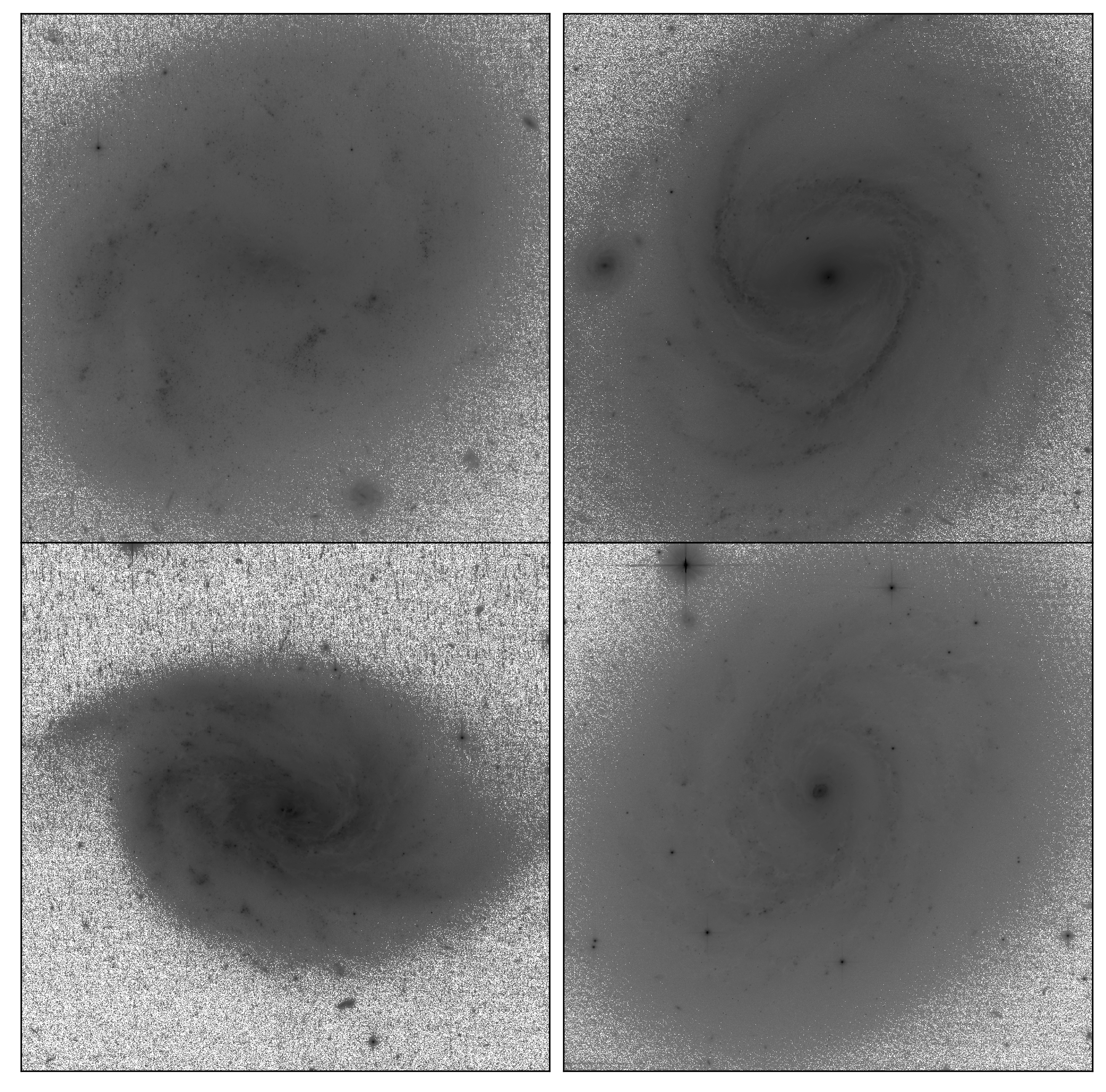
Figure 8: Four of the galaxies with HST ACS imaging used in our tests of image registration. From top to bottom and left to right the galaxies are NGC1483, NGC1577, NGC1803, and NGC2216. The panels are all 80 arcsecs in vertical and horizontal extent.

The second HST dataset is an archival image of the nearby spiral galaxy NGC2841, taken using the WFC3/UVIS instrument (HST proposal ID 11360, PI R. O’Connell) The galaxy in this case is significantly closer, and has $\sim 7$ times more resolved elements than the mean for the other HST images used.

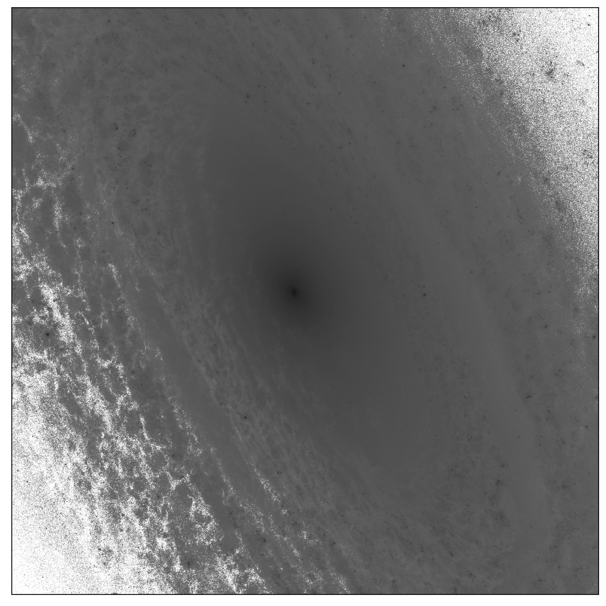
Figure 9: HST/WFC3 image of the region of the nearby spiral galaxy NGC 2841, used for our tests of galaxy image registration. The image is a square of side length 160 arcsecs.

Galaxy ID	minor axis radius (arcsec)	redshift	$r$ magnitude
NGC1483	30.1	0.0039	12.26
NGC1577	72.0	0.0312	13.0
NGC1803	40.8	0.0136	12.54
NGC2216	48.6	0.0091	12.34
NGC2841	238.8	0.00190	9.88

Table 2: Physical properties of galaxies with HST imaging used in our tests (images are shown in Figures 8 and 9). Data is from the NASA Extragalactic Database ( https://ned.ipac.caltech.edu/ ) and the CDS SIMBAD database (https://simbad.u-strasbg.fr ).

To carry out tests with galaxies that have few resolution elements, our third dataset consists of galaxy images taken from the ground based SDSS telescope. The NASA-Sloan atlas is a catalogue of images (see e.g., Maller et al. (2009) and parameters of local galaxies derived from SDSS imaging, and with the addition of Galaxy Evolution Explorer (GALEX) data for the ultraviolet part of the spectrum. We do not use the UV data, but as with the HST data above we restrict ourselves to a single filter image per galaxy (in the SDSS $r$ band). We choose 12 spiral or irregular galaxies randomly in each of three bins of Petrosian radius, 3-5 arcsec, 10-30 arcsec and 70-80 arcsec. Some example galaxies in each of these three bins are shown in Figure 10. In the case of the NSA galaxies, the seeing will determine the size of the resolution elements. The mean SDSS $r$ band imaging seeing is 1.32 arcsec FWHM, and for simplicity we use this value for all NSA images. The SDSS pixel size is 0.40 arcsecs.

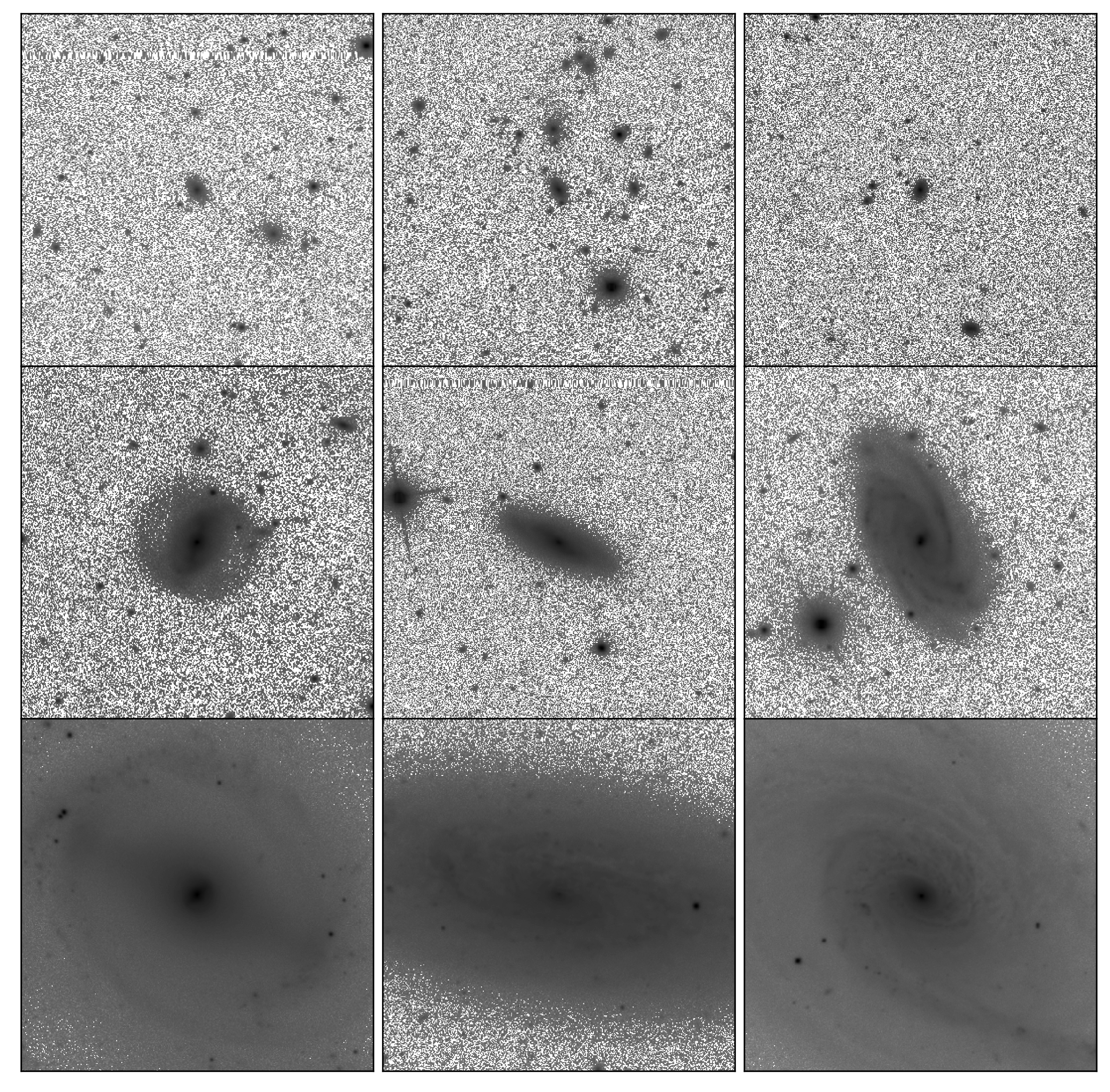
Figure 10: Examples of galaxy images from the NASA Sloan Atlas used for our tests of image registration. The top row shows galaxies with Petrosian radius between 3 and 5 arcsecs, middle row 10-30 arcsecs, and bottom row 70-80 arcsec. All images are 160 arcsecs in diameter.

A.3 Method

For each galaxy image, we first select a circular region within two Petrosian radii of the galaxy centroid in the case of the NSA data, and two times the minor axis radius in the case of the large HST galaxies. The number of resolution elements in the galaxy is then computed using Equation 6. In the case of NGC 2841, we split this region into separate square chunks of side length 400 pixels, in order to test the effect of using mosaic images. Our results for this galaxy are averaged over all chunks.

We shift each galaxy image by a distance in the $x$ and $y$ directions drawn from uniform random distributions between -10 and +10 pixels. The image shift is carried out in Fourier space, using the Python routine scipy.ndimage.fourier_shift . We restrict ourselves in these tests to rigid translations, leaving rotations and deformations to future work.

The next step is to add noise to each of the images (shifted and unshifted). We do this by Poisson sampling the image with discrete photons. In order to make sure that we are in the Poisson limited regime, we simulate short exposures, using an effective exposure time of one second for the NSA images (compared to the SDSS single exposure time of 54 seconds). This leads to a mean number of photons per resolution element of 200. To be consistent and allow comparison across the different galaxy datasets and angular sizes, we also scale the effective exposure time of the HST images so that the mean number of photons per resolution element is also 200.

At this point, we have two noisy images of the same galaxy and would like to estimate the image shift. In our case, we have introduced a shift which is a rigid translation. There are a number of methods which can be employed to determine the shift, and the literature on this topic is growing (e.g., Wang et al. 2018 ). We use a simple Fourier method, based on publicly available software, the astropy image registration package. The specific routine we use is chi2_shift . This is based on the single step Discrete Fourier Transform algorithm from Guizar et al. (2008). The algorithm uses the entire image to compute the upsampled cross-correlation in Fourier space in a small neighborhood around its peak. This allows rapid subpixel registration, but has not been shown to be an optimal method.

We carry out the process 100 times for each galaxy image, with different photon sampling and image shifts each time, and then compute the rms error on the detected shift.

A.4 Results

In Figure 11 we show the rms error on the measured translational shifts, $\sigma_{\rm astro}$ as points for each galaxy, as a function of $N_{\rm elem}$, the number of resolution elements. In order to plot both HST and NSA galaxies on the same graph, we have converted the NSA results from arcsec into pixels and then into arcsec at the resolution of HST. The mean number of photons per resolution element was also the same for all galaxies, as described above.

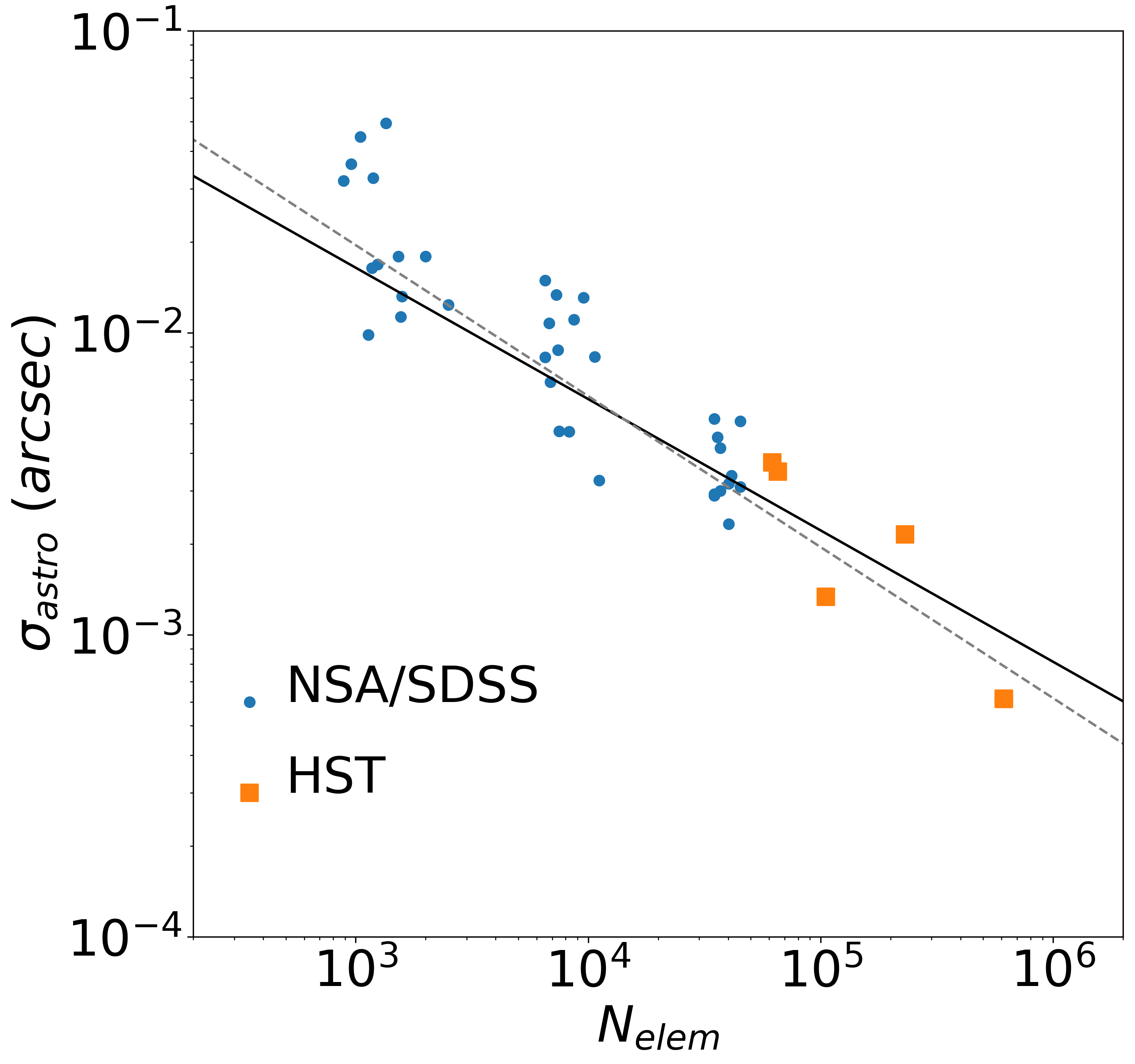
Figure 11: The rms error, $\sigma_{\rm astro}$ on measurements of galaxy image shifts using Fourier space image registration techniques plotted as a function of the number of resolved elements in each individual galaxy, $N_{\rm elem}$ (computed using Equation 6). We show results for the HST images as orange squares and the ground based data from SDSS as blue points. The solid line is a best fit to all points, and has a slope $\sigma_{\rm astro}\propto N_{\rm elem}^{-0.440\pm 0.025}$. The dashed line is the ideal scaling, $\sigma_{\rm astro}\propto N_{\rm elem}^{-0.5}$.

We can see that the accuracy of shift measurement increases with the number of resolution elements, although there is significant scatter. We have carried out a least squares fit of the best fit power law (with residuals in log $\sigma_{\rm astro}$, using the Python routine scipy.optimize.curve_fit), and find the slope to be $-0.440\pm 0.025$. We show this best fit line on Figure 11 as a solid line. We also show in Figure 11 a dashed line corresponding to the case where $\sigma_{\rm astro}\propto N_{\rm elem}^{-0.5}$, which we have assumed in our analyses in the main text. We can see that this is somewhat steeper than the fit relationship, but only at the $2.4\sigma$ level. Real galaxies do not therefore appear to behave very much differently than our assumptions in the text, at least as far as these simple tests show.

A.5 Discussion

We have carried out some simple tests with observational data to find the accuracy with which galaxy image shifts can be detected. We have found that the positions of larger galaxies, spanned by more resolution elements can indeed be found more accurately than smaller galaxies. The absolute value of the slope of the relationship between the number of elements and rms measurement error is slightly less than the the ideal value of 0.5, which was used in our predictions in the main text. We have decided not to change the fiducial value in the text, because the tests here are merely illustrative, and many questions remain to be answered (see below).

Our tests have been limited to the shot noise dominated regime, with high noise levels, due to the necessity to avoid conflating noise features in the test data with real structure. This is obviously the easiest regime to simulate, but has meant that we have not been able to test the extremely small image shifts that will be present in Rubin and Roman data. These shifts will be far below our test shifts (for example, the point source measurement error for NGRST is $\sim 2.5\times 10^{-5}$ arcsecs). Also, there will be systematic errors that enter, including field distortions, colour/filter effects, charge transfer effects and more. A more sophisticated treatment will need to deal with these.

Another important aspect that we have not touched are the magnitudes of the errors themselves. We have restricted ourselves to relative comparisons between different sized galaxies under the same conditions. There are two reasons for this, the first being that different techniques for image registration of extended objects at the sub pixel level could perform much better or worse than others. For example, Hrazdíra et al. (2020) have shown how recently developed iterative methods can offer substantial improvements on some prior methods. The second is that although it would obviously be useful to compare the accuracy to that of centroiding point sources (particularly since the point source rms errors are what is quoted for the telescopes of interest), simulating point sources in this context is non-trivial. For point source tests, one would need to model a realistic background, detection of sources themselves, and determine how non-detections would affect the errors. We leave these and other complexities to future work.

In the main text, we have discussed that a reference frame will need to be set up for cosmic parallax measurements based on extremely distant galaxies (for example at distances greater than 1 Gpc from the observer, where parallaxes will not be measurable). We have seen that the number density of distant galaxies is expected to be high enough that the errors from setting the frame will be very subdominant. We have not addressed this issue in our tests, but have instead assumed measurements of galaxy image shifts with respect to a constant reference frame defined by pixel axes. We have also only addressed rigid translation of images. In reality, there will be there will be other rigid transformations (rotations), as well as affine (shears for example), homographies, or more complex large deformations. Image registration techniques used will have to deal with these. There is therefore much that has been left to future work.

References

- Abbott et al. (2017) Abbott B. P., et al., 2017, Phys. Rev. Lett., 119, 161101
- Abell et al. (2009) Abell P. A., et al., 2009, arXiv e-prints arXiv:0912.0201,
- Abitbol et al. (2020) Abitbol M. H., Hill J. C., Chluba J., 2020, ApJ, 893, 18
- Ade et al. (2014) Ade P. A. R., et al., 2014, A&A, 571, A16
- Akrami et al. (2020) Akrami Y., et al., 2020, arXiv e-prints arXiv:2003.12646,
- Bahcall & Kulier (2014) Bahcall N. A., Kulier A., 2014, MNRAS, 439, 2505
- Bailer-Jones et al. (2018) Bailer-Jones C. A. L., Rybizki J., Fouesneau M., Mantelet G., Andrae R., 2018, AJ, 156, 58
- Behroozi et al. (2013) Behroozi P. S., Wechsler R. H., Wu H.-Y., 2013, ApJ, 762, 109
- Beutler et al. (2011) Beutler F., et al., 2011, MNRAS, 416, 3017
- Binney & Merrifield (1998) Binney J., Merrifield M., 1998, Galactic Astronomy. Princeton
- Blanton et al. (2005) Blanton M. R., Eisenstein D., Hogg D. W., Schlegel D. J., Brinkmann J., 2005, ApJ, 629, 143
- Boehm et al. (2017) Boehm C., et al., 2017, arXiv e-prints arXiv:1707.01348,
- Bonifacio et al. (2016) Bonifacio P., et al., 2016, in Reylé C., Richard J., Cambrésy L., Deleuil M., Pécontal E., Tresse L., Vauglin I., eds, SF2A-2016: Proceedings of the Annual meeting of the French Society of Astronomy and Astrophysics. pp 267–270
- Branchini et al. (1999) Branchini E., et al., 1999, MNRAS, 308, 1
- Brown et al. (2018) Brown A. G. A., et al., 2018, A&A, 616, A1
- Carlesi et al. (2016) Carlesi E., et al., 2016, MNRAS, 458, 900
- Chen et al. (2019) Chen G. C. F., et al., 2019, MNRAS, 490, 1743
- Chisari et al. (2019) Chisari N. E., et al., 2019, ApJS, 242, 2
- Colombi et al. (2007) Colombi S., Chodorowski M. J., Teyssier R., 2007, MNRAS, 375, 348
- Conroy et al. (2006) Conroy C., Wechsler R. H., Kravtsov A. V., 2006, ApJ, 647, 201
- Croft & Dailey (2011) Croft R. A. C., Dailey M., 2011, arXiv e-prints arXiv:1112.3108,
- Croft & Gaztanaga (1997) Croft R. A. C., Gaztanaga E., 1997, MNRAS, 285, 793
- Crossland et al. (2020) Crossland T., Stenetorp P., Riedel S., Kawata D., Kitching T. D., Croft R. A. C., 2020, MNRAS, 492, 3217
- Cuceu et al. (2019) Cuceu A., Farr J., Lemos P., Font-Ribera A., 2019, J. Cosmology Astropart. Phys., 2019, 044
- Darling (2012) Darling J., 2012, ApJ, 761, L26
- Darling & Truebenbach (2018) Darling J., Truebenbach A. E., 2018, ApJ, 864, 37
- Darling et al. (2018) Darling J., Truebenbach A. E., Paine J., 2018, ApJ, 861, 113
- Davis et al. (2011) Davis T. M., et al., 2011, ApJ, 741, 67
- Dhawan et al. (2018) Dhawan S., Jha S. W., Leibundgut B., 2018, A&A, 609, A72
- Ding & Croft (2009) Ding F., Croft R. A. C., 2009, MNRAS, 397, 1739
- Freedman et al. (2001) Freedman W. L., et al., 2001, ApJ, 553, 47
- Freedman et al. (2019) Freedman W. L., et al., 2019, ApJ, 882, 34
- Ghez et al. (2008) Ghez A. M., et al., 2008, ApJ, 689, 1044
- Gorski et al. (1989) Gorski K. M., Davis M., Strauss M. A., White S. D. M., Yahil A., 1989, ApJ, 344, 1
- Graham (2019) Graham M., 2019, in The Extragalactic Explosive Universe: the New Era of Transient Surveys and Data-Driven Discovery. p. 23, doi:10.5281/zenodo.3478038
- Graham et al. (2018) Graham M. L., Connolly A. J., Ivezić Ž., Schmidt S. J., Jones R. L., Jurić M., Daniel S. F., Yoachim P., 2018, AJ, 155, 1
- Gramann et al. (1994) Gramann M., Cen R., Gott J. Richard I., 1994, ApJ, 425, 382
- Graziani et al. (2019) Graziani R., Courtois H. M., Lavaux G., Hoffman Y., Tully R. B., Copin Y., Pomarède D., 2019, MNRAS, 488, 5438
- Guizar et al. (2008) Guizar M., Thurman S., Fienup J., 2008, Optics Letters, 33, 156
- Hall (2019) Hall A., 2019, MNRAS, 486, 145
- Hinshaw et al. (2009) Hinshaw G., et al., 2009, ApJS, 180, 225
- Hoffman & Ribak (1991) Hoffman Y., Ribak E., 1991, ApJ, 380, L5
- Hogg (1999) Hogg D. W., 1999, arXiv e-prints astro-ph/9905116,
- Holz & Hughes (2005) Holz D. E., Hughes S. A., 2005, ApJ, 629, 15
- Howlett & Davis (2020) Howlett C., Davis T. M., 2020, MNRAS, 492, 3803
- Hrazdíra et al. (2020) Hrazdíra Z., Druckmüller M., Habbal S., 2020, ApJS, 247, 8
- Hubble (1925) Hubble E. P., 1925, ApJ, 62, 409
- Huchra (1992) Huchra J. P., 1992, Science, 256, 321
- Ishiyama et al. (2015) Ishiyama T., Enoki M., Kobayashi M. A. R., Makiya R., Nagashima M., Oogi T., 2015, PASJ, 67, 61
- Ivesić et al. (2018) Ivesić Z., et al., 2018, LSST document LPM-17, pp LPM–17
- Ivezić et al. (2012) Ivezić Ž., Beers T. C., Jurić M., 2012, ARA&A, 50, 251
- Kardashev et al. (1973) Kardashev N. S., Parijskij Y. N., Umarbaeva N. D., 1973, Astrofizicheskie Issledovaniia Izvestiya Spetsial’noj Astrofizicheskoj Observatorii, 5, 16
- Keselman & Nusser (2017) Keselman J. A., Nusser A., 2017, MNRAS, 467, 1915
- Kogut et al. (1993) Kogut A., et al., 1993, ApJ, 419, 1
- Kopeikin & Makarov (2006) Kopeikin S. M., Makarov V. V., 2006, AJ, 131, 1471
- Korzyński & Kopiński (2018) Korzyński M., Kopiński J., 2018, J. Cosmology Astropart. Phys., 2018, 012
- Kuglin & Hines (1975) Kuglin C. D., Hines D. C., 1975, Proc. Int. Conference on Cybernetics and Society. IEEE, p. 163–165
- Lange & Page (2007) Lange S., Page L., 2007, ApJ, 671, 1075
- Lindegren et al. (2018) Lindegren L., et al., 2018, A&A, 616, A2
- Loeb (1998) Loeb A., 1998, ApJ, 499, L111
- Makiya et al. (2016) Makiya R., et al., 2016, PASJ, 68, 25
- Maller et al. (2009) Maller A. H., Berlind A. A., Blanton M. R., Hogg D. W., 2009, ApJ, 691, 394
- Marshall et al. (2017) Marshall P., et al., 2017, arXiv e-prints arXiv:1708.04058,
- McCrea (1935) McCrea W. H., 1935, Z. Astrophys., 9, 290
- Méndez et al. (2011) Méndez R. A., Costa E., Gallart C., Pedreros M. H., Moyano M., Altmann M., 2011, AJ, 142, 93
- Mukherjee et al. (2019) Mukherjee S., Lavaux G., Bouchet F. R., Jasche J., Wandelt B. D., Nissanke S. M., Leclercq F., Hotokezaka K., 2019, arXiv e-prints arXiv:1909.08627,
- Nicolaou et al. (2019) Nicolaou C., Lahav O., Lemos P., Hartley W., Braden J., 2019, arXiv e-prints, p. arXiv:1909.09609
- Paine et al. (2020) Paine J., Darling J., Graziani R., Courtois H. M., 2020, ApJ, 890, 146
- Quercellini et al. (2012) Quercellini C., Amendola L., Balbi A., Cabella P., Quartin M., 2012, Phys. Rep., 521, 95
- Refsdal (1966) Refsdal S., 1966, MNRAS, 132, 101
- Riess (2019) Riess A. G., 2019, Nature Reviews Physics, 2, 10
- Riess et al. (2005) Riess A. G., et al., 2005, ApJ, 627, 579
- Riess et al. (2019) Riess A. G., Casertano S., Yuan W., Macri L. M., Scolnic D., 2019, ApJ, 876, 85
- Sandage (1962) Sandage A., 1962, ApJ, 136, 319
- Sanderson et al. (2017) Sanderson R. E., et al., 2017, Astrometry with the Wide-Field InfraRed Space Telescope (arXiv:1712.05420)
- Schlegel et al. (2015) Schlegel D., et al., 2015, in APS April Meeting Abstracts. p. Z2.006
- Simard et al. (1999) Simard L., et al., 1999, ApJ, 519, 563
- Spergel et al. (2013) Spergel D., et al., 2013, arXiv e-prints arXiv:1305.5422,
- Springob et al. (2014) Springob C. M., et al., 2014, MNRAS, 445, 2677
- Starr et al. (2002) Starr B. M., et al., 2002, LSST Instrument Concept. Society of Photo-Optical Instrumentation Engineers (SPIE) Conference Series, pp 228–239, doi:10.1117/12.457331
- Tolman (1934) Tolman R. C., 1934, Relativity, Thermodynamics, and Cosmology. Dover, New York
- Tully et al. (2016) Tully R. B., Courtois H. M., Sorce J. G., 2016, AJ, 152, 50
- Tyson et al. (2003) Tyson J. A., Wittman D. M., Hennawi J. F., Spergel D. N., 2003, Nuclear Physics B Proceedings Supplements, 124, 21
- Vasiliev (2019) Vasiliev E., 2019, MNRAS, 489, 623
- Verde et al. (2019) Verde L., Treu T., Riess A. G., 2019, Nature Astronomy, 3, 891–895
- Wang et al. (2018) Wang S., Quan D., Liang X., Ning M., Guo Y., Jiao L., 2018, ISPRS Journal of Photogrammetry and Remote Sensing, 145, 148
- Wang et al. (2020) Wang Y., Li B., Cautun M., 2020, MNRAS, 497, 3451
- Weinberg (1972) Weinberg S., 1972, Gravitation and Cosmology: Principles and Applications of the General Theory of Relativity. Wiley
- Willick & Batra (2001) Willick J. A., Batra P., 2001, ApJ, 548, 564
- Yu & Zhu (2019) Yu Y., Zhu H.-M., 2019, ApJ, 887, 265
- Zitova & Flusser (2003) Zitova B., Flusser J., 2003, Image and Vision Computing, 11 edn. Elsevier, p. 977–1000
- da Silva et al. (2019) da Silva R., et al., 2019, Euclid Near-infrared Imaging Reduction Pipeline: Astrometric Calibration, Resampling and Stacking. p. 311