Attribution Analysis of Grammatical Dependencies in LSTMs

Abstract

LSTM language models have been shown to capture syntax-sensitive grammatical dependencies such as subject–verb agreement with a high degree of accuracy (Linzen et al., 2016, inter alia). However, questions remain regarding whether they do so using spurious correlations, or whether they are truly able to match verbs with their subjects. This paper argues for the latter hypothesis. Using layer-wise relevance propagation (Bach et al., 2015), a technique that quantifies the contribution of input features to model behavior, we show that LSTM performance on number agreement is directly correlated with the model's ability to distinguish subjects from other nouns. Our results suggest that LSTM language models are able to infer robust representations of syntactic dependencies.

1 Introduction

A major area of research in interpretable NLP concerns the question of whether black-box models are capable of inferring complex grammatical dependencies from data. Linzen et al. (2016) approached this question by constructing a diagnostic task based on subject–verb agreement whose solution requires knowledge of natural language syntax. Since this seminal work, the basic methodology has been extended in several ways. These include hand-crafting testing sets to control for linguistic features (Marvin and Linzen, 2018; Wilcox et al., 2018; Warstadt et al., 2019); extracting information from network layers using diagnostic classification (Giulianelli et al., 2018; Lin et al., 2019); and detecting representations of syntactic structure through unsupervised parsing (Merrill et al., 2019).

Methodologies based on task and testing set design demonstrate that models exhibit behavior consistent with that of a fully interpretable model, and methodologies based on extracting representations demonstrate that model weights contain enough information to represent some aspect of natural language grammar. Supplementing these approaches, we propose the use of attribution analysis, a methodology that enables us to directly determine the reasoning by which a model arrives at a certain decision. In attribution analysis, each input to a model is assigned a score measuring the importance of that input in determining the model's output. Interpretable models should assign high scores to input features that are relevant for computing the output, while those that assign high scores to irrelevant features are likely to be ``Clever Hans predictors'' (Lapuschkin et al., 2019)—models that primarily rely on spurious correlations to optimize their training objectives.

This paper adopts layer-wise relevance propagation (LRP, Bach et al., 2015), an attribution method that distributes logit scores among model inputs, and applies it to Linzen et al.'s (2016) subject–verb agreement task. Using Marvin and Linzen's (2018) Targeted Syntactic Evaluation (TSE), a partitioned testing set that controls for syntactic structure, we show that the performance of LSTM language models on subject–verb agreement is directly correlated with the degree to which subjects are assigned higher scores than other words, while failure to exhibit this phenomenon results in degraded performance. These results show that our model enforces agreement by matching verbs with their subjects, and not by relying on idiosyncratic statistical properties of the training data.

This paper is structured as follows. Sections 2 and 3 review LRP and the relevant literature on attribution analysis. Section 4 describes our experimental procedure, and Section 5 presents our results. These results are discussed in Section 6, and Section 7 concludes.

2 Layer-Wise Relevance Propagation

LRP assigns to each input of a network a relevance score representing its contribution to the model output. To understand what this means, let us consider an illustrative example.

Example .

Suppose Alice holds two part-time positions. She works for $x$ hours in position 1 at the rate of $$p/\text{hour}$ and $y$ hours in position 2 at the rate of $$q/\text{hour}$. Alice's total income is given by the function

$$f(x,y)=t(px+qy),$$

where $t$ is a non-linear function mapping Alice's gross income to her post-tax income.

LRP asks the following question: how much of Alice's income comes from position 1 and how much comes from position 2? It is clear that $$px$ of Alice's pre-tax income comes from position 1 and $$qy$ comes from position 2. Intuitively, we may attribute Alice's total income to the two positions in the same proportions. Thus, the amount of money Alice has earned from position 1 is

$$R(x)=f(x,y)\cdot\frac{px}{px+qy},$$

and the amount earned from position 2 is

$$R(y)=f(x,y)\cdot\frac{qy}{px+qy}.$$

We can apply this reasoning to LSTMs using the following derivation, due to Arras et al. (2017). Consider an LSTM classifier that takes inputs $\mathbf{x}_{1},\allowbreak\mathbf{x}_{2},\allowbreak\dots,\allowbreak\mathbf{x}_{t}$ and passes the final hidden state $\mathbf{h}_{t}$ through a linear layer, producing a vector $\mathbf{y}$ of logit scores. We initialize the relevance $R(\mathbf{y})$ of the output layer by

$$R(\mathbf{y})=\operatorname{argmax}(\mathbf{y}).$$

We seek to determine the contribution of each input $\mathbf{x}_{i}$ to the logit score $\mathbf{1}^{\top}R(\mathbf{y})$ of the predicted class. We do this by propagating the relevance value backwards through the network, applying the reasoning of Example 2 repeatedly.

To begin, we propagate $R(\mathbf{y})$ to the final hidden state $\mathbf{h}_{t}$ and the linear layer bias term $\mathbf{b}$. Following the the reasoning of Example 2, the relevance of each term is determined by the proportion of $\mathbf{y}$ comprised by that term.

$$R(\mathbf{h}_{t})=R(\mathbf{y})\odot\frac{\mathbf{W}\mathbf{h}_{t}}{\mathbf{y}}=R(\mathbf{y})\odot\frac{\mathbf{W}\mathbf{h}_{t}}{\mathbf{W}\mathbf{h}_{t}+\mathbf{b}}$$

Recall that $\mathbf{h}_{t}$ is given by

$$\mathbf{h}_{t} =\mathbf{o}_{t}\odot\tanh(\mathbf{c}_{t})$$

$$=\mathbf{o}_{t}\odot\tanh(\mathbf{f}_{t}\odot\mathbf{c}_{t-1}+\mathbf{i}_{t}\odot\mathbf{g}_{t}),$$ (1)

where $\mathbf{c}_{t}$ is the cell state and $\mathbf{f}_{t}$, $\mathbf{i}_{t}$, and $\mathbf{o}_{t}$ are the forget gate, input gate, and output gate, respectively. Following Arras et al. (2017), we treat the output gate $\mathbf{o}_{t}$ as a unary operator $\mathbf{v}\mapsto\mathbf{o}_{t}\odot\mathbf{v}$, so that (1) may be viewed as a linear mapping with activation $\mathbf{o}_{t}\odot\tanh(\cdot)$. Example 2 then gives us

$$R(\mathbf{i}_{t}\odot\mathbf{g}_{t})=R(\mathbf{h}_{t})\odot\frac{\mathbf{i}_{t}\odot\mathbf{g}_{t}}{\mathbf{f}_{t}\odot\mathbf{c}_{t-1}+\mathbf{i}_{t}\odot\mathbf{g}_{t}}.$$

Next, we rewrite $\mathbf{i}_{t}\odot\mathbf{g}_{t}$ as a linear mapping with activation $\mathbf{i}_{t}\odot\tanh(\cdot)$:

$$\mathbf{i}_{t}\odot\mathbf{g}_{t}=\mathbf{i}_{t}\odot\tanh(\mathbf{W}_{g,x}\mathbf{x}_{t}+\mathbf{W}_{g,h}\mathbf{h}_{t-1}+\mathbf{b}_{g}).$$

By Example 2,

$$R(\mathbf{x}_{t})=R(\mathbf{i}_{t}\odot\mathbf{g}_{t})\odot\frac{\mathbf{W}_{g,x}\mathbf{x}_{t}}{\mathbf{W}_{g,x}\mathbf{x}_{t}+\mathbf{W}_{g,h}\mathbf{h}_{t-1}+\mathbf{b}_{g}}$$

and

$$\mathrel{\phantom{=}}R(\mathbf{h}_{t-1})$$

$$=R(\mathbf{i}_{t}\odot\mathbf{g}_{t})\odot\frac{\mathbf{W}_{g,h}\mathbf{h}_{t-1}}{\mathbf{W}_{g,x}\mathbf{x}_{t}+\mathbf{W}_{g,h}\mathbf{h}_{t-1}+\mathbf{b}_{g}}.$$

This completes the backwards relevance propagation for one time step of the LSTM. To compute the relevance propagation for the next time step, we notice from (1) that both $\mathbf{h}_{t}$ and $\mathbf{h}_{t-1}$ propagate relevance to $\mathbf{c}_{t-1}$. To account for this, we decompose (1) into two separate equations:

$$\mathbf{h}_{t-1} =\mathbf{o}_{t-1}\odot\tanh(\mathbf{c}_{t-1})$$ (2)

$$\mathbf{c}_{t-1} =\mathbf{f}_{t-1}\odot\mathbf{c}_{t-2}+\mathbf{i}_{t-1}\odot\mathbf{g}_{t-1}.$$ (3)

(2) is a one-term linearity with activation $\mathbf{o}_{t-1}\odot\tanh(\cdot)$, while (3) is a linear equation with identity activation. We compute $R(\mathbf{c}_{t-1})$ by summing the contributions from $\mathbf{h}_{t}$ and $\mathbf{h}_{t-1}$:

$$R(\mathbf{c}_{t-1})=R(\mathbf{c}_{t})\odot\frac{\mathbf{f}_{t}\odot\mathbf{c}_{t-1}}{\mathbf{c}_{t}}+R(\mathbf{h}_{t-1});$$

and we continue the computation using (3):

$$R(\mathbf{i}_{t-1}\odot\mathbf{g}_{t-1})=R(\mathbf{c}_{t-1})\odot\frac{\mathbf{i}_{t-1}\odot\mathbf{g}_{t-1}}{\mathbf{c}_{t-1}}.$$

LRP relevance scores have the following desirable conservation property. Suppose $f$ is a neural network that takes inputs $x_{1},x_{2},\dots,x_{m}\in\mathbb{R}$ and produces outputs $y_{1},y_{2},\dots,y_{n}\in\mathbb{R}$. Then,

$$\sum_{i=1}^{n}R(y_{i})=\left(\sum_{i=1}^{m}R(x_{i})\right)+\sum_{b\in B}R(b),$$ (4)

where $B$ is the set of bias units of $f$. This allows us to assign a scalar relevance value $r(U)$ to any collection of units $U$ by taking the sum $r(U)=\sum_{u\in U}R(u)$. For example, the collective relevance of inputs $\mathbf{x}_{1}$ and $\mathbf{x}_{2}$ is $r(\mathbf{x}_{1},\mathbf{x}_{2})=\mathbf{1}^{\top}(R(\mathbf{x}_{1})+R(\mathbf{x}_{2}))$. In the LSTM setting, (4) then becomes

$$\max_{i}y_{i}=r(\mathbf{y})=\left(\sum_{j=1}^{t}r(\mathbf{x}_{j})\right)+\sum_{b\in B}r(b).$$ (5)

3 Related Work

A variety of techniques exist for attribution analysis. LRP, along with DeepLIFT (Shrikumar et al., 2017), takes the approach of propagating a signal backwards through the network. Other methods, such as saliency analysis (Simonyan et al., 2014; Li et al., 2016), gradient $\odot$ input (Denil et al., 2015), and integrated gradients (Sundararajan et al., 2017a, b), involve computing model gradients, based on the intuition that model outputs should not be affected by changes in irrelevant features. Finally, techniques like contextual decomposition (Murdoch et al., 2018) and LIMSSE (Poerner et al., 2018) involve computing local linear approximations of the model or certain parts thereof.

Arras et al. (2019) have argued, on the basis of toy tasks, that LRP yields more intuitive explanations for NLP than other techniques. We choose to use LRP for two reasons. Firstly, relevance scores may be positive or negative, allowing us to distinguish features that contribute to a model decision from those that inhibit against it. Secondly, the additive property of relevance scores allows us to aggregate relevance scores across inputs of varying lengths, enabling us to qualitatively compare model computations on different kinds of inputs without resorting to inspection of cherry-picked examples.

Attribution analysis is traditionally applied to sentiment analysis (e.g., Li et al., 2016; Murdoch et al., 2018; Arras et al., 2017), where the intrinsic sentiment value of input words gives attribution scores a natural interpretation. Poerner et al. (2018) apply a number of attribution methods to Linzen et al.'s (2016) subject–verb agreement task. Whereas we use attribution analysis to assess whether models behave in an interpretable way, Poerner et al. assume that models behave in an interpretable way and evaluate attribution methods based on their ability to reveal this interpretable behavior. Like Arras et al. (2019), they conclude that LRP delivers more interpretable explanations than other methods.

4 Experimental Procedure

Name	Template	Example
Simple	Det1 N1	The senators laugh
Inside an Object Relative Clause (IORC)	Det2 N2 (Comp) Det1 N1	The manager (that) the skater admires
Sentential Complement (SC)	Det2 N2 V Det1 N1	The mechanic said the manager laughs
Across a PP (PP)	Det1 N1 P Det2 N2	The surgeon in front of the ministers laughs
Across a Subject Relative Clause (SRC)	Det1 N1 Comp V Det2 N2	The customer that hates the dancer laughs
Across an Object Relative Clause (ORC)	Det1 N1 (Comp) Det2 N2 V	The officers (that) the parents hate laugh
Short VP Coordination (SVP)	Det1 N1 V Conj	The farmers smile and swim
Long VP Coordination (LVP)	Det1 N1 V CompVP Conj	The senator knows many different foreign
		languages and is

Table 1: TSE templates for subject–verb agreement.

Our experimental approach combines attribution analysis with the Targeted Syntactic Evaluation (TSE) paradigm of Marvin and Linzen (2018). In TSE, models are evaluated using a testing set partitioned into subsets consisting of inputs generated from rigid syntactic templates. Model performance is then compared across the templates, revealing challenging inputs for the model. In this study, we rely on the structural rigidity imposed by the templates to aggregate LRP computations over collections of inputs.

All evaluations in this study are computed using the best-performing English language model from Gulordava et al. (2018), which is available for download from the authors' website. Previous work applying TSE to LSTMs, including Marvin and Linzen (2018), Shen et al. (2019), and Kuncoro et al. (2019), use models trained using the same data, vocabulary, and hyperparameters as Gulordava et al. The remainder of this section reviews the TSE paradigm (Subsection 4.1) and introduces our LRP evaluation scheme (Subsections 4.2 and 4.3).

4.1 Targeted Syntactic Evaluation

TSE attempts to probe a model's syntactic knowledge through a series of diagnostic tasks. We focus here on subject–verb agreement. Test examples for subject–verb agreement are given by word sequences like (4.1). The keys on the table *is/are (4.1) is a sentence truncated at a verb. In this example, the verb agrees with the noun keys, and therefore must take the plural form are and not the singular form is. In TSE, the words preceding the verb, known as the preamble, are given to the language model as input, and we compare the probability scores assigned to the singular and plural forms of the verb. If the appropriate form receives a higher score, we consider the model to have correctly predicted the number of the verb.

The templates for subject–verb agreement are shown in Table 1. We describe each template as a sequence of part-of-speech (POS) tags: Complementizer, Conjunction, Determiner, Noun, Preposition, Verb, or Complement of Verb Phrase. We label the subject of each preamble that triggers agreement on the target verb and its associated determiner with the tags N1 and Det1, respectively, and we label all other nouns and determiners with N2 and Det2, respectively. The complementizer that appearing in the ORC and IORC templates is optional.

We make two changes to Marvin and Linzen's (2018) original testing set for agreement. Firstly, the original testing set contains distinct sentences that are identical up to the preamble and the target verb, resulting in duplicate test cases. We remove those duplicate cases from our testing set. Secondly, the original testing set is completely in lowercase, even though the vocabulary is case-sensitive. We modify our testing set by capitalizing the first letter of each sentence. We will see in Section 5 that capitalization substantially increases our model's prediction accuracy for most templates. Although these changes render our prediction accuracies incomparable to previously reported results, we expect that the improvement in performance will lead to more interpretable explanations from the LRP analysis.

4.2 LRP Evaluation

In Section 2, we considered LSTM classifiers, and initialized $R(\mathbf{y})$ to $\operatorname{argmax}(\mathbf{y})$, so that $\mathbf{1}^{\top}R(\mathbf{y})$ is the highest logit score produced by the model. In the current task, we are interested in comparing the logit score assigned to one possible next word with the score assigned to another possible word. Therefore, we initialize $R(\mathbf{y})$ so that $\mathbf{1}^{\top}R(\mathbf{y})$ is the difference $\Delta y$ between the two scores in question. For example, when evaluating the test case given by (4.1), $R(\mathbf{y})$ is initialized as follows:

$$R(\mathbf{y})_{i}=\begin{cases}y_{i},&i=\text{are}\\ -y_{i},&i=\text{is}\\ 0,&\text{otherwise.}\end{cases}$$

Observe that $\mathbf{1}^{\top}R(\mathbf{y})=y_{\text{are}}-y_{\text{is}}=\Delta y$.

For each POS tag in each template, we compute the collective scalar relevance score of all words subsumed under that tag. For example, given the preamble The surgeon in front of the ministers, we assign the P tag the relevance score $r(\text{P})=r(\text{in},\text{front},\text{of})$. For an input $\mathbf{x}$, $|r(\mathbf{x})|$ represents the magnitude of $\mathbf{x}$'s contribution to $\Delta y$, and the sign of $r(\mathbf{x})$ indicates whether $\mathbf{x}$ increases $\Delta y$ or decreases it.

4.3 Pointing Game Accuracy

Intuitively, we would expect that an interpretable model should assign high-magnitude attribution scores to N1 and scores close to 0 for words unrelated to subject–verb agreement. Based on this idea, Poerner et al. (2018) propose the pointing game accuracy as a way to induce a quantitative measure of interpretability from an attribution method. The pointing game accuracy of a model on a testing set for the agreement task is the percentage of test cases for which N1 receives the highest attribution score. Here, we compute pointing game accuracy on TSE templates using the absolute value of relevance scores.

5 Results

Prediction Accuracy	Simple	IORC	IORC	SC	PP	SRC	ORC	ORC	SVP	LVP
		(No That)					(No That)
Marvin and Linzen (2018)	94	71	84	99	57	56	52	50	90	61
Shen et al. (2019)	100	81	88	98	68	60	51	52	92	74
Kuncoro et al. (2019)	100	86	90	97	89	87	70	77	96	82
Our Model (Capitalized)	100	85	90	96	84	87	57	69	99	81
Our Model (Lowercase)	100	85	90	100	65	68	52	59	94	80
Pointing Game	Simple	IORC	IORC	SC	PP	SRC	ORC	ORC	SVP	LVP
		(No That)					(No That)
Pointing Game Accuracy	65	56	54	55	32	46	20	16	25	23
N2	–	15	23	11	28	21	29	22	–	–

Table 2: Top: Number prediction accuracies attained by our model, compared with previously reported results for similar models. Bottom: Pointing game accuracies attained by our model, along with the percentage of examples in which N2 received the highest-magnitude relevance score.

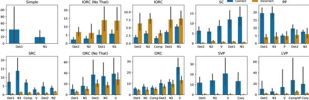
Figure 1: The absolute values of relevance scores assigned to template positions by our language model for correct (blue, left) and incorrect (orange, right) predictions.

The upper portion of Table 2 presents our replication of Marvin and Linzen's (2018) results. As mentioned in Subsection 4.1, capitalization improves the performance of our model on all templates except for SC and IORC. We attribute this to the fact that The appears almost exclusively sentence-initially while the almost never appears sentence-initially; we hypothesize that this difference in distribution provides heuristic information about which nouns are likely to be subjects. While our results are not directly comparable with previous ones, note that our model performs similarly to Kuncoro et al. (2019) on the capitalized inputs and Shen et al. (2019) on the lowercase inputs.

Figure 1 shows the absolute-value relevance scores assigned to POS tags for each template. Inputs for which the model makes a correct number prediction are plotted separately from those for which the model makes an incorrect prediction. The following subsections discuss the ability of our model to identify subjects (5.1), the role of determiners in number prediction (5.2), the effect of polysemy on model behavior (5.3), and an alternate strategy for agreement using verb coordination (5.4).

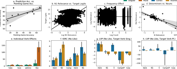
Figure 2: a: The relationship between pointing game accuracy and prediction accuracy ($\rho=\text{0.65}$). b: The relationship between N1 relevance and the logit score of the correct verb form ($\rho=\text{0.46}$). c: The effect of frequency on relevance ($\rho=-\text{0.08}$). d: The relationship between N relevance and Det relevance ($\rho=-\text{0.73}$). e: The absolute values of relevance scores assigned to individual verbs in ORC, plotted by their number. f: The absolute values of relevance scores for IORC inputs, excluding examples where the target verb is like(s). g and h: Signed relevance scores for LVP sentences without like(s), plotted according to the number of the target verb.

5.1 Identifying Subjects

The goal of this subsection is to determine whether our model makes number predictions by identifying the subject of its input, or whether it exhibits Clever Hans behavior. Figure 1 shows that in most cases, $|r(\text{N1})|>|r(\text{N2})|$ when the model makes a correct number prediction, and vice versa. When the model makes incorrect predictions, $|r(\text{N2})|$ is closer to $|r(\text{N1})|$, indicating that these are situations in which the model does not confidently distinguish one noun from the other.

There are two exceptions to this pattern. In IORC, we have $|r(\text{N1})|>|r(\text{N2})|$ even when the network makes incorrect predictions, and in ORC, we have $|r(\text{N2})|>|r(\text{N1})|$ even when the network makes correct predictions. We will see in Subsection 5.3 that the IORC phenomenon is due to the polysemous nature of the target verb like(s), which is amply present in the test set. With ORC, we note that our model achieves the lowest performance on this template, with an average accuracy of 66% on inputs both with and without the complementizer that.

In Figure 2a, we see that pointing game accuracy on templates is positively correlated with prediction accuracy, with a Pearson correlation coefficient of $\rho=\text{0.65}$. Similarly, the percentage of inputs matching a given template for which N2 receives the highest-magnitude relevance score is negatively correlated with prediction accuracy, with $\rho=-\text{0.65}$. This suggests that the ability to identify N1 and distinguish it from N2 is an important factor in determining the model's ability to perform number prediction. Overall, Figure 2b shows that $\log(|r(\text{N1})|)$ is correlated with the logit score of the correct verb form, while Figure 2c shows that word frequency in the training set, a possible source of spurious correlation, has no significant effect on relevance.

5.2 Determiners

A striking observation about Figure 1 is that $|r(\text{Det1})|$ and $|r(\text{Det2})|$ are often greater than or close to $|r(\text{N1})|$ and $|r(\text{N2})|$, respectively. This phenomenon is unexpected, since the determiner The/the, which is the only possible value for Det1 and Det2, does not carry agreement information.

Figure 2d shows that $r(\text{N})$ is negatively correlated with $r(\text{Det})$. The regression line gives us

$$r(\text{Det},\text{N})=\text{0.287}r(\text{N})+\text{0.642},$$

which indicates that when The/the is combined with a noun, it asymptotically has the effect of scaling the relevance of the resulting noun phrase by a factor of roughly 0.3. The regression line predicts that $r(\text{Det},\text{N})$ may have the opposite sign of $r(\text{N})$ when $-\text{2.235}<r(\text{N})<\text{0}$. In this region, the negative relevance of N is overruled by the positive relevance of Det. This occurs in 22% of cases, and we will later see that it plays an important role in the LVP template.

5.3 Verbs and Polysemy

Template	All Inputs	No Like
IORC (No That)	85	93
IORC	90	94
SRC	87	88
ORC (No That)	57	58
ORC	69	71
LVP	81	95

(a) Prediction accuracies with inputs containing like(s) removed. Simple, SC, PP, and SVP do not have any inputs with like(s).

V	CompVP
know(s)	many different foreign languages
like(s)	to watch television shows
is/are	twenty three years old
enjoy(s)	playing tennis with colleagues
write(s)	in a journal every day

(b) Values for V and CompVP in LVP inputs.

Table 3:

Template	Likes	Like	Other
IORC (No That)	0	63	37
IORC	0	55	45
LVP	9	29	62

Table 4: The percentage of incorrect predictions where the predicted verb is likes, like, or some other verb.

On average, ORC predictions assign the highest-magnitude relevance scores to V. In correct predictions without that, this relevance magnitude is disproportionately high, with $|r(\text{V})|\approx\text{2}\cdot|r(\text{N2})|$. Considering the relevance magnitudes assigned to individual verb types, Figure 2e reveals that the plural form like receives far more relevance than other verbs. Intuitively, the fact that like can be used as a verb, preposition, noun, or adjective means that this particular form conveys information to the model that is not conveyed by the other verb forms, affecting its behavior.

3(a) shows that for all templates using the verb like(s), model performance improves when examples containing like(s) are omitted. SRC and ORC experience modest improvements, while IORC and LVP improve substantially. The former two contain like(s) in the preamble, but not in the target verb; IORC contains like(s) in the target verb, but not in the preamble; and LVP contains like(s) both in the target verb and in the preamble. This indicates that including like(s) as the target verb is a major source of errors in number prediction. Intuitively, the polysemy of like means that it may appear in more contexts than its singular counterpart likes. For example, like a brother… is a reasonable continuation of The customer that loves the dancer in which like is used as a preposition. The existence of these alternatives may therefore bias the model in favor of predicting like over likes. This is indeed borne out in Table 4: the model is far more likely to incorrectly predict like than likes for LVP, and the model never incorrectly predicts likes for IORC. Whereas Figure 1 showed that IORC anomalously exhibits $|r(\text{N1})|>|r(\text{N2})|$ when making incorrect predictions, in Figure 2f we see that this behavior is entirely due to the bias toward like.

5.4 Coordination

Two templates with prominently low pointing game accuracies are SVP and LVP. Here, V and the conjunction and receive high-magnitude relevance scores. We interpret the model to be relying on the fact that coordinated verbs generally agree with the same subject, and therefore bear the same number agreement morphology. Thus, these templates present an example in which the model employs a robust alternative strategy that does not necessarily require identifying N1, but instead obtains number features from the verb.

Figures 2g and 2h present a more detailed analysis of LVP, excluding examples involving like(s). In most cases, CompVP receives a negative relevance score, which is offset by $r(\text{Det1},\text{N1},\text{V})$. As shown in 3(b), CompVP always contains at least one noun, which may be either singular or plural, thus distracting the model with confounding agreement information. The model makes incorrect predictions when $r(\text{V})$ is too close to 0 to offset $r(\text{CompVP})$. Observe that $r(\text{V})$ by itself is not large enough to completely offset $r(\text{CompVP})$: it is only able to do so by combining with $r(\text{Det1},\text{N1})$. Thus, while N1 does not receive the highest-magnitude relevance scores, it is still important for ensuring correct model behavior. When the target verb is singular, $r(\text{N1})$ is slightly negative; but because its magnitude is small enough to lie within the $-\text{2.235}<r(\text{N1})<\text{0}$ zone, $r(\text{Det1})$ reverses its directionality. In this situation, we may understand Det1 to provide a correction for the case where $r(\text{N1})$ is negative but close to 0. Finally, in addition to Det1, N1, V, and CompVP, the conjunction and often receives a high-magnitude relevance score. In Figure 2h we see that this score is only positive when the target verb is plural. Thus, we may view and as providing a plural bias to the network, possibly arising from the inherent plurality of coordinated subjects.

6 Discussion

The analysis we have presented reveals several key insights about LSTM behavior. Owing to the additive nature of both LRP and the cell state update equation, we may view LSTMs as devices that accumulate information extracted from inputs. Our model's ability to make correct predictions is determined by its ability to weigh information about N1 with information about N2. The IORC, SC, PP, and SRC templates, which consist of two noun phrases with some material in between, show that the model is able to adjust the relative prominence of the two noun phrases to fit the syntactic context. This behavior is also seen with determiners, which serve to adjust the magnitude and sometimes the direction of the relevance introduced by nouns. Finally, as we have seen with LVP, the model is able to combine information from multiple sources to justify one decision over another.

Our observation that $|r(\text{N1})|$ is often close to $|r(\text{N2})|$ when the model makes incorrect predictions is consistent with two findings of Giulianelli et al. (2018) regarding the encoding of agreement information in the hidden state vector $\mathbf{h}_{t}$. Firstly, Giulianelli et al. claim that agreement errors are often due to misencodings of the subject. This is reflected in our framework by the fact that incorrect predictions often result in a smaller N1 relevance (e.g., in the PP template), indicating that the model has failed at least in part to extract number information from N1. Secondly, Giulianelli et al. observe that when making incorrect predictions, $\mathbf{h}_{t}$ loses its number encoding after the second noun has been processed. This may be explained by the additive nature of relevance: if $|r(\text{N1})|\approx|r(\text{N2})|$ in a sentence where N1 and N2 bear opposite number features, then we expect that $r(\text{N1})+r(\text{N2})\approx\text{0}$. Thus, the agreement information extracted from N1 neutralizes the information extracted from N2.

No explanation has been offered in Section 5 for the relevance scores of the ORC template. Given that both V and N2 receive high-magnitude relevance scores even though they transmit the same agreement information, model behavior on this template is likely determined entirely by N2. Thus, we conclude that our model cannot handle the ORC construction, and that its slight improvement over chance is due to Clever Hans behavior.

7 Conclusion

Our analysis has shown that the LSTM language model of Gulordava et al. (2018) enforces subject–verb agreement in an interpretable manner. While the model draws number information from several sources, including nouns, verbs, and and, identifying the target verb's subject is crucial to the model's ability to execute the agreement task, even in cases where it is used in conjunction with evidence from other inputs. In the case where the model is unable to identify the subject, namely ORC, the model only slightly outperforms chance. These findings demonstrate that the successes of the LSTM language model on the agreement task are not due to Clever Hans behavior.

The methodological approach we have taken in this study is based on the synthesis of two existing methodologies: experimentally controlled testing sets and attribution analysis. Both components are required for our approach. For instance, while Poerner et al. (2018) report a pointing game accuracy of 86% in their number prediction study, it is difficult to discern the significance of this number on its own without further context. By correlating pointing game accuracy with prediction accuracy on different kinds of testing sets, however, we can determine the extent to which model behavior results from executing the desired strategy. Thus, combining multiple analytical techniques may prove to be a fruitful way to gain insights beyond what is revealed by standard evaluation metrics.

Although we have argued that positive results about the grammatical abilities of LSTMs are not due to Clever Hans behavior, we have not shown that LSTMs are able to infer stack-like representations of hierarchical syntactic structure or memory-bounded approximations thereof. While TSE introduces syntactic complexity by incorporating a diversity of constructions, the TSE templates are generally quite simple in terms of embedding depth and dependency length. As discussed in Section 6, most of the templates are superficially similar to one another even if they are represented differently in linguistic theory. Among the rest, LVP features a long-distance dependency between the target verb and N1, while ORC features a center-embedding construction. The model's promising performance on LVP and failure on ORC seems to suggest that depth is more challenging for the model than distance. Such issues provide avenues of exploration for future work.

References

- Arras et al. (2017) Leila Arras, Grégoire Montavon, Klaus-Robert Müller, and Wojciech Samek. 2017. Explaining Recurrent Neural Network Predictions in Sentiment Analysis. In Proceedings of the 8th Workshop on Computational Approaches to Subjectivity, Sentiment and Social Media Analysis, pages 159–168, Copenhagen, Denmark. Association for Computational Linguistics.
- Arras et al. (2019) Leila Arras, Ahmed Osman, Klaus-Robert Müller, and Wojciech Samek. 2019. Evaluating Recurrent Neural Network Explanations. In Proceedings of the 2019 ACL Workshop BlackboxNLP: Analyzing and Interpreting Neural Networks for NLP, pages 113–126, Florence, Italy. Association for Computational Linguistics.
- Bach et al. (2015) Sebastian Bach, Alexander Binder, Grégoire Montavon, Frederick Klauschen, Klaus-Robert Müller, and Wojciech Samek. 2015. On Pixel-Wise Explanations for Non-Linear Classifier Decisions by Layer-Wise Relevance Propagation. PLOS ONE, 10(7):e0130140.
- Denil et al. (2015) Misha Denil, Alban Demiraj, and Nando de Freitas. 2015. Extraction of Salient Sentences from Labelled Documents. Computing Research Repository, arXiv:1412.6815.
- Giulianelli et al. (2018) Mario Giulianelli, Jack Harding, Florian Mohnert, Dieuwke Hupkes, and Willem Zuidema. 2018. Under the Hood: Using Diagnostic Classifiers to Investigate and Improve how Language Models Track Agreement Information. In Proceedings of the 2018 EMNLP Workshop BlackboxNLP: Analyzing and Interpreting Neural Networks for NLP, pages 240–248, Brussels, Belgium. Association for Computational Linguistics.
- Gulordava et al. (2018) Kristina Gulordava, Piotr Bojanowski, Edouard Grave, Tal Linzen, and Marco Baroni. 2018. Colorless Green Recurrent Networks Dream Hierarchically. In Proceedings of the 2018 Conference of the North American Chapter of the Association for Computational Linguistics: Human Language Technologies, volume 1, pages 1195–1205, New Orleans, LA. Association for Computational Linguistics.
- Kuncoro et al. (2019) Adhiguna Kuncoro, Chris Dyer, Laura Rimell, Stephen Clark, and Phil Blunsom. 2019. Scalable Syntax-Aware Language Models Using Knowledge Distillation. In Proceedings of the 57th Annual Meeting of the Association for Computational Linguistics, pages 3472–3484, Florence, Italy. Association for Computational Linguistics.
- Lapuschkin et al. (2019) Sebastian Lapuschkin, Stephan Wäldchen, Alexander Binder, Grégoire Montavon, Wojciech Samek, and Klaus-Robert Müller. 2019. Unmasking Clever Hans predictors and assessing what machines really learn. Nature Communications, 10(1):1096.
- Li et al. (2016) Jiwei Li, Xinlei Chen, Eduard Hovy, and Dan Jurafsky. 2016. Visualizing and Understanding Neural Models in NLP. In Proceedings of the 2016 Conference of the North American Chapter of the Association for Computational Linguistics: Human Language Technologies, pages 681–691, San Diego, CA. Association for Computational Linguistics.
- Lin et al. (2019) Yongjie Lin, Yi Chern Tan, and Robert Frank. 2019. Open Sesame: Getting inside BERT's Linguistic Knowledge. In Proceedings of the 2019 ACL Workshop BlackboxNLP: Analyzing and Interpreting Neural Networks for NLP, pages 241–253, Florence, Italy. Association for Computational Linguistics.
- Linzen et al. (2016) Tal Linzen, Emmanuel Dupoux, and Yoav Goldberg. 2016. Assessing the Ability of LSTMs to Learn Syntax-Sensitive Dependencies. Transactions of the Association for Computational Linguistics, 4(0):521–535.
- Marvin and Linzen (2018) Rebecca Marvin and Tal Linzen. 2018. Targeted Syntactic Evaluation of Language Models. In Proceedings of the 2018 Conference on Empirical Methods in Natural Language Processing, pages 1192–1202, Brussels, Belgium. Association for Computational Linguistics.
- Merrill et al. (2019) William Merrill, Lenny Khazan, Noah Amsel, Yiding Hao, Simon Mendelsohn, and Robert Frank. 2019. Finding Hierarchical Structure in Neural Stacks. In Proceedings of the 2019 ACL Workshop BlackboxNLP: Analyzing and Interpreting Neural Networks for NLP, pages 224–232, Florence, Italy.
- Murdoch et al. (2018) W. James Murdoch, Peter J. Liu, and Bin Yu. 2018. Beyond Word Importance: Contextual Decomposition to Extract Interactions from LSTMs. In ICLR 2018 Conference Track, Vancouver, Canada. OpenReview.
- Poerner et al. (2018) Nina Poerner, Hinrich Schütze, and Benjamin Roth. 2018. Evaluating neural network explanation methods using hybrid documents and morphosyntactic agreement. In Proceedings of the 56th Annual Meeting of the Association for Computational Linguistics, volume 1: Long Papers, pages 340–350, Melbourne, Australia. Association for Computational Linguistics.
- Shen et al. (2019) Yikang Shen, Shawn Tan, Alessandro Sordoni, and Aaron Courville. 2019. Ordered Neurons: Integrating Tree Structures into Recurrent Neural Networks. In ICLR 2019 Conference Track, New Orleans, LA. OpenReview.
- Shrikumar et al. (2017) Avanti Shrikumar, Peyton Greenside, and Anshul Kundaje. 2017. Learning Important Features Through Propagating Activation Differences. In Proceedings of the 34th International Conference on Machine Learning, volume 70 of Proceedings of Machine Learning Research, pages 3145–3153, Sydney, Australia. PMLR.
- Simonyan et al. (2014) Karen Simonyan, Andrea Vedaldi, and Andrew Zisserman. 2014. Deep Inside Convolutional Networks: Visualising Image Classification Models and Saliency Maps. In ICLR 2014 Workshop Proceedings, Banff, Canada. arXiv.
- Sundararajan et al. (2017a) Mukund Sundararajan, Ankur Taly, and Qiqi Yan. 2017a. Axiomatic Attribution for Deep Networks. In Proceedings of the 34th International Conference on Machine Learning, volume 70 of Proceedings of Machine Learning Research, pages 3319–3328, Sydney, Australia. PMLR.
- Sundararajan et al. (2017b) Mukund Sundararajan, Ankur Taly, and Qiqi Yan. 2017b. Axiomatic Attribution for Deep Networks. Computing Research Repository, arXiv:1703.01365v2.
- Warstadt et al. (2019) Alex Warstadt, Yu Cao, Ioana Grosu, Wei Peng, Hagen Blix, Yining Nie, Anna Alsop, Shikha Bordia, Haokun Liu, Alicia Parrish, Sheng-Fu Wang, Jason Phang, Anhad Mohananey, Phu Mon Htut, Paloma Jeretic, and Samuel R. Bowman. 2019. Investigating BERT's Knowledge of Language: Five Analysis Methods with NPIs. In Proceedings of the 2019 Conference on Empirical Methods in Natural Language Processing and the 9th International Joint Conference on Natural Language Processing (EMNLP-IJCNLP), pages 2877–2887, Hong Kong, China. Association for Computational Linguistics.
- Wilcox et al. (2018) Ethan Wilcox, Roger Levy, Takashi Morita, and Richard Futrell. 2018. What do RNN Language Models Learn about Filler–Gap Dependencies? In Proceedings of the 2018 EMNLP Workshop BlackboxNLP: Analyzing and Interpreting Neural Networks for NLP, pages 211–221, Brussels, Belgium. Association for Computational Linguistics.