A Population-Informed Mass Estimate for Pulsar J0740+6620

Abstract

Galactic double neutron star systems have a tight mass distribution around $\sim 1.35M_{\odot}$, but the mass distribution of all known pulsars is broader (Tauris et al., 2017). Here we reconstruct the Alsing et al. (2018); Antoniadis et al. (2016) bimodal mass distribution of pulsars observed in binary systems, incorporating data from observations of J0740+6620 which were not available at the time of those works. Because J0740+6620 is an outlier in the mass distribution with non-negligible uncertainty in its mass measurement, its mass receives a large correction from the population, becoming $m_{J0740+6620{}}=2.03^{+0.10}_{-0.08}\,M_{\odot}$ (median and 68% CI). Stochastic samples from our population model, including population-informed pulsar mass estimates, are available at https://github.com/farr/AlsingNSMassReplication.

1 The Pulsar Mass Distribution

There are three classes of pulsar mass measurements used in Alsing et al. (2018). The first consist of well-constrained pulsar mass measurements, where the likelihood function is assumed to be (proportional to) a Gaussian:

$$p\left(d_{p}\mid m_{p}\right)\propto\exp\left(-\frac{\left(m_{p}-\mu\right)^{2}}{2\sigma^{2}}\right),$$ (1)

with $d_{p}$ the (abstract) pulsar measurement “data,” and $m_{p}$ the true mass of the pulsar. Here $\mu$ is the reported mass measurement and $\sigma$ is its uncertainty. The second class consists of measurements of the mass function,

$$f\equiv\frac{m_{p}q^{3}\sin^{2}\iota}{\left(1+q\right)^{2}},$$ (2)

where $q=m_{c}/m_{p}$ ($m_{c}$ is the companion mass; this implies $0<q<\infty$) and $\iota$ is the angle between the orbital angular momentum and the line of sight; $f$ is assumed to be measured perfectly (uncertainties on $f$ are below the part-per-thousand level, and therefore ignorable); and measurements of the total mass of the binary system, $m_{t}=m_{p}\left(1+q\right)$ with an assumed Gaussian likelihood centered at the measured total mass, $\mu_{t}$, with standard deviation $\sigma_{t}$. The complete likelihood is

$$p\left(d_{p}\mid m_{p},m_{t},\iota\right)\propto\delta\left(f\left(m_{p},m_{t},\iota\right)-f_{p}\right)\exp\left(-\frac{\left(m_{t}-\mu_{t}\right)^{2}}{2\sigma_{t}^{2}}\right),$$ (3)

with $f_{p}$ the measured mass function. Integrating over $\iota$ with an isotropic prior (flat in $\cos\iota$) leaves the marginal likelihood

$$p\left(d_{p}\mid m_{p},m_{t}\right)\propto\exp\left(-\frac{\left(m_{t}-\mu_{t}\right)^{2}}{2\sigma_{t}^{2}}\right)\frac{m_{t}^{4/3}}{3\left(m_{t}-m_{p}\right)^{2}f_{p}^{1/3}\sqrt{1-\frac{f_{p}^{2/3}m_{t}^{4/3}}{\left(m_{t}-m_{p}\right)^{2}}}}$$ (4)

(compare Alsing et al. (2018) Eq. (3)). The third class consists of systems with (perfect) measurements of the mass function and Gaussian uncertainties on the mass ratio, $q$; similarly, integrating over $\iota$ with an isotropic prior leads to a marginal likelihood

$$p\left(d_{p}\mid m_{p},q\right)\propto\exp\left(-\frac{\left(q-\mu_{q}\right)^{2}}{2\sigma_{q}^{2}}\right)\frac{\left(1+q\right)^{4/3}}{3f_{p}^{1/3}m_{p}^{2/3}q^{2}\sqrt{1-\left(\frac{f_{p}}{m_{p}}\right)^{2/3}\frac{\left(1+q\right)^{4/3}}{q^{2}}}};$$ (5)

this is Eq. (4) with $m_{t}\to m_{p}\left(1+q\right)$ in the term that arises from integrating over $\iota$; notably, this differs from Alsing et al. (2018) Eq. (4).

For our analysis, we extend the Alsing et al. (2018) data set to include the Cromartie et al. (2020) measurement of J0740+6620 with $\mu=2.14\,M_{\odot}$ and $\sigma=0.1\,M_{\odot}$.

We fit a pulsar population model to this data set with

$$p\left(m_{p}\mid A,m_{\mathrm{max}},\mu_{1,2},\sigma_{1,2}\right)=\\ \begin{cases}A\alpha\exp\left(-\frac{\left(m_{p}-\mu_{1}\right)^{2}}{2\sigma_{1}^{2}}\right)+\left(1-A\right)\beta\exp\left(-\frac{\left(m_{p}-\mu_{2}\right)^{2}}{2\sigma_{2}^{2}}\right)&0<m_{p}\leq m_{\mathrm{max}}\\ 0&\textnormal{otherwise}\end{cases},$$ (6)

where $\alpha=\alpha\left(m_{\mathrm{max}},\mu_{1},\sigma_{1}\right)$ and $\beta=\beta\left(m_{\mathrm{max}},\mu_{2},\sigma_{2}\right)$ normalize the Gaussian terms in the sum to individually integrate to 1 for $0<m_{p}\leq m_{\mathrm{max}}$ so that $A$ is the fraction of the population in the first Gaussian component. This is equivalent to the Alsing et al. (2018) model with $n=2$ Gaussian components. We impose that $\mu_{1}<\mu_{2}$ to break labeling degeneracy. We use the Stan sampler (Carpenter et al., 2017a) to sample over the pulsar population parameters, pulsar masses, and total masses or mass ratios (for the appropriate subset of pulsars). We use the same priors as Alsing et al. (2018) on the pulsar-level parameters. Our code and samples, as well as the LaTeX source for this document can be found at https://github.com/farr/AlsingNSMassReplication.

An example of our results for the pulsar population are found in the left panel of Fig. 1, where we show the distribution of pulsar masses marginalized over the posterior for the distribution parameters and the posterior on the $m_{\mathrm{max}}$ parameter; similarly to Alsing et al. (2018), we find that the pulsar mass distribution tapers off for $m_{p}\gtrsim 2\,M_{\odot}$, either because there is a sharp cutoff ($m_{\mathrm{max}}\simeq 2\,M_{\odot}$), leading to a peak in the posterior for $m_{\mathrm{max}}$ near $2\,M_{\odot}$, or because the second Gaussian component is narrow and $m_{\mathrm{max}}$ is unconstrained, leading to the “tail” in $m_{\mathrm{max}}$ running up to $3\,M_{\odot}$. We find somewhat weaker evidence for a sharp cutoff than reported in Alsing et al. (2018) with the Bayes Factor in favor of a cutoff varying between 1:1 and 5:1 depending on the choice of $m_{\mathrm{max}}$ prior.

2 Updated Mass Estimate for J0740+6620

We report an updated mass estimate for J0740+6620 informed by this population analysis. The Cromartie et al. (2020) mass estimate is an outlier relative to the distribution, with an uncertainty $\sigma_{m}\simeq 0.1\,M_{\odot}$ comparable to the overall pulsar distribution width $\sigma_{2}\simeq 0.25\,M_{\odot}$, and therefore receives a large “correction” from the joint distribution (Fishbach et al., 2020). We find $m_{J0740+6620{}}=2.03{}^{+0.10{}}_{-0.08{}}\,M_{\odot}$ (median and symmetric 68% credible interval) when incorporating a population model for galactic pulsars similar to Alsing et al. (2018), right panel of Fig. 1. The updated mass estimate for J0740+6620 is informed by the population analysis of galactic pulsar mass measurements. These include double neutron star binaries, neutron star-white dwarf binaries, and X-ray binaries. Most heavy pulsars with precise mass measurements are in neutron star-white dwarf binaries; it is these systems that control the mass distribution near $m_{p}\simeq 2\,M_{\odot}$. J0740+6620 is also of this type, so the systems with the strongest effect on the “correction” to the J0740+6620 mass are likely the most similar among the set of pulsars considered here.

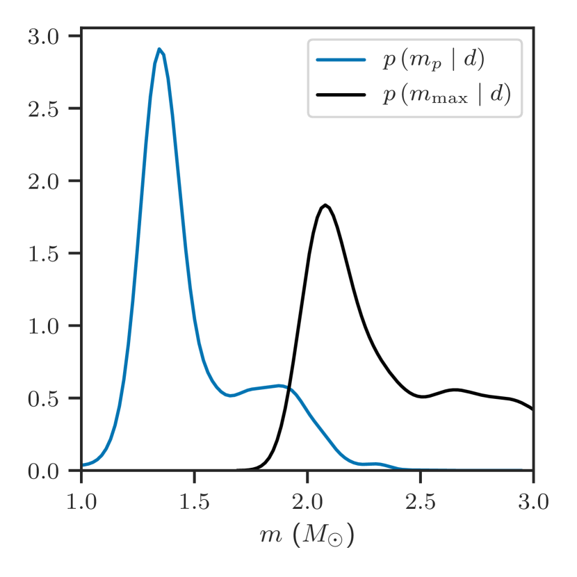
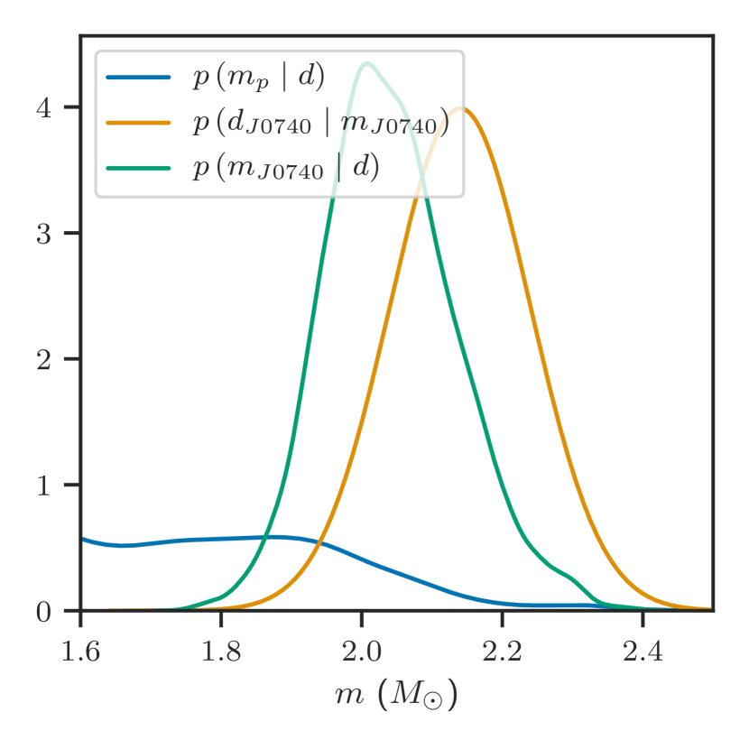
Figure 1: Left: Posterior predictive distribution—the mass distribution obtained by marginalizing over all pulsar parameters and population-level parameters in Eq. (6) given the complete data set—for the pulsar mass distribution (blue) and posterior for the maximum mass (black). Right: Likelihood for the mass of J0740+6620 assuming only data for that pulsar (orange) and the posterior on its mass obtained from marginalization of the joint posterior on all pulsar parameters and population parameters from the population inference based on the entire data set of galactic pulsar mass measurements (green). The tail of the pulsar mass distribution from the left figure is also shown in blue; because the tail tapers strongly over the range of masses supported by the J0740+6620 likelihood the population-informed mass estimate is “pulled” to lower values.

References

- Alsing et al. (2018) Alsing, J., Silva, H. O., & Berti, E. 2018, MNRAS, 478, 1377, doi: 10.1093/mnras/sty1065
- Antoniadis et al. (2016) Antoniadis, J., Tauris, T. M., Ozel, F., et al. 2016. https://arxiv.org/abs/1605.01665
- Astropy Collaboration (2013) Astropy Collaboration. 2013, Astronomy and Astrophysics, 558, A33, doi: 10.1051/0004-6361/201322068
- Carpenter et al. (2017a) Carpenter, B., Gelman, A., Hoffman, M., et al. 2017a, Journal of Statistical Software, Articles, 76, 1, doi: 10.18637/jss.v076.i01
- Carpenter et al. (2017b) —. 2017b, Journal of Statistical Software, Articles, 76, 1, doi: 10.18637/jss.v076.i01
- Cromartie et al. (2020) Cromartie, H. T., Fonseca, E., Ransom, S. M., et al. 2020, Nature Astronomy, 4, 72, doi: 10.1038/s41550-019-0880-2
- Fishbach et al. (2020) Fishbach, M., Farr, W. M., & Holz, D. E. 2020, ApJ, 891, L31, doi: 10.3847/2041-8213/ab77c9
- Hunter (2007) Hunter, J. D. 2007, Computing In Science & Engineering, 9, 90, doi: 10.1109/MCSE.2007.55
- Kumar et al. (2019) Kumar, R., Carroll, C., Hartikainen, A., & Martin, O. A. 2019, The Journal of Open Source Software, doi: 10.21105/joss.01143
- Oliphant (2006) Oliphant, T. 2006, NumPy: A guide to NumPy, USA: Trelgol Publishing. http://www.numpy.org/
- Price-Whelan et al. (2018) Price-Whelan, A. M., et al. 2018, American Astronomical Society, 156, 123, doi: 10.3847/1538-3881/aabc4f
- Tauris et al. (2017) Tauris, T., et al. 2017, Astrophys. J., 846, 170, doi: 10.3847/1538-4357/aa7e89
- The Pandas Development Team (2020) The Pandas Development Team. 2020, pandas-dev/pandas: Pandas, latest, Zenodo, doi: 10.5281/zenodo.3509134
- Virtanen et al. (2020) Virtanen, P., et al. 2020, Nature Methods, 17, 261, doi: https://doi.org/10.1038/s41592-019-0686-2
- Waskom et al. (2020) Waskom, M., Botvinnik, O., Ostblom, J., et al. 2020, mwaskom/seaborn: v0.10.1 (April 2020), v0.10.1, Zenodo, doi: 10.5281/zenodo.3767070