Abstract

Motivated by a simultaneous explanation of the apparent discrepancies in the light charged lepton anomalous magnetic dipole moments, and the anomalous internal pair creation in ⁸Be nuclear transitions, we explore a simple New Physics model, based on an extension of the Standard Model gauge group by a $U(1)_{B-L}$. The model further includes heavy vector-like fermion fields, as well as an extra scalar responsible for the low-scale breaking of $U(1)_{B-L}$, which gives rise to a light $Z^{\prime}$ boson. The new fields and currents allow to explain the anomalous internal pair creation in ⁸Be while being consistent with various experimental constraints. Interestingly, we find that the contributions of the $Z^{\prime}$ and the new $U(1)_{B-L}$-breaking scalar can also successfully account for both $(g-2)_{e,\mu}$ anomalies; the strong phenomenological constraints on the model’s parameter space ultimately render the combined explanation of $(g-2)_{e}$ and the anomalous internal pair creation in ⁸Be particularly predictive. The underlying idea of this minimal “prototype model” can be readily incorporated into other protophobic $U(1)$ extensions of the Standard Model.

1 Introduction

The possible existence of new interactions, in addition to those associated with the Standard Model (SM) gauge group, has been a longstanding source of interest, both for particle and astroparticle physics. Numerous experimental searches have been dedicated to look for theoretically well-motivated light mediators, such as axions (spin-zero), dark photons (spin-1) or light $Z^{\prime}$ (spin-1) [1, 2, 3, 4, 5, 6, 7, 8, 9, 10, 11, 12, 13, 14, 15, 16, 17, 18, 19, 20, 21, 22, 23, 24, 25, 26, 27, 28, 29, 30, 31, 32, 33, 34, 35, 36, 37, 38, 39, 40].

Several distinct probes have been used to look for the presence of the new mediators. Nuclear transitions are among the most interesting and promising laboratories to search for relatively light new physics states. A few years ago, the Atomki Collaboration reported their results [41] on the measurement of the angular correlation of electron-positron internal pair creation (IPC) for two nuclear transitions of Beryllium atoms (⁸Be), with a significant excess being observed at large angles for one of them. The magnetic dipole ($M1$) transitions under study concerned the decays of the excited isotriplet and isosinglet states, respectively denoted ⁸Be${}^{*^{\prime}}$ and ⁸Be^∗, into the fundamental state (⁸Be⁰). The transitions are summarised below, together with the associated energies:

$${}^{8}\text{Be}^{*^{\prime}}(j^{\pi}=1^{+},T=1)\,\rightarrow\,^{8}\text{Be}^{0}(j^{\pi}=0^{+},T=0)\,,\quad E\,=\,17.64\text{ MeV}\,;$$

$${}^{8}\text{Be}^{*}(j^{\pi}=1^{+},T=0)\,\rightarrow\,^{8}\text{Be}^{0}(j^{\pi}=0^{+},T=0)\,,\quad E\,=\,18.15\text{ MeV}\,,$$ (1)

in which $j^{\pi}$ and $T$ correspond to the spin-parity and isospin of the nuclear states, respectively. A significant enhancement of the IPC was observed at large angles in the angular correlation of the 18.15 MeV transition; it was subsequently pointed out that such an anomalous result could be potentially interpreted as the creation and decay of an unknown intermediate light particle with mass $m_{X}$=16.70$\pm 0.35$(stat)$\pm 0.5$(sys) MeV [41] .

Recently, a re-investigation of the ⁸Be anomaly with an improved set up corroborated the earlier results for the 18.15 MeV transition [42, 43, 44, 45]; moreover, it allowed constraining the mass of the hypothetical mediator to $m_{X}=17.01(16)$ MeV and its branching ratio (normalised to the $\gamma$-decay) to $\Gamma_{X}/\Gamma_{\gamma}=6(1)\times 10^{-6}$. The $e^{+}e^{-}$ pair correlation in the 17.64 MeV transition of ⁸Be was also revisited, and again no significant anomalies were found [46, 47]. A combined interpretation of the data of ${}^{8}\text{Be}^{*}$ decays (only one set exhibiting an anomalous behaviour) in terms of a new light particle, in association with the possibility of mixing between the two different excited ⁸Be isospin states (${}^{8}\text{Be}^{*^{\prime}}$ and ${}^{8}\text{Be}^{*}$) might suggest a larger preferred mass for the new mediator; this would lead to a large phase space suppression, therefore potentially explaining the null results for ${}^{8}\text{Be}^{*^{\prime}}$ decay. In turn, it can further entail significant changes in the preferred quark (nucleon) couplings to the new particle mediating the anomalous IPC, corresponding to significantly smaller normalised branching fractions than those of the preferred fit of [48].

Further anomalies in nuclear transitions have been observed, in particular concerning the 21.01 MeV $0^{-}\rightarrow 0^{+}$ transition of ⁴He [48, 49], resulting in another anomalous IPC corresponding to the angular correlation of electron-positron pairs at 115^∘, with 7.2$\sigma$ significance. The result can also be potentially interpreted as the creation and subsequent decay of a light particle: the corresponding mass and width, $m_{X}$=16.98$\pm 0.16\text{(stat)}\pm 0.20(\text{syst})$ MeV, and $\Gamma_{X}$= $3.9\times 10^{-5}$ eV, lie in a range similar to that suggested by the anomalous ${}^{8}\mathrm{Be}$ transition.

If the anomalous IPC observations are to be interpreted as being mediated by a light new state, the latter can a priori be a scalar, pseudoscalar, vector, axial vector, or even a spin-2 particle, provided it decays into electron-positron pairs. For a parity conserving scenario, the hypothesis of an intermediate scalar boson has already been dismissed [51], due conservation of angular momentum in the $1^{+}\rightarrow 0^{+}$ ⁸Be transition. Having a pseudoscalar mediator has been also severely constrained (and disfavoured) by experiments – for an axion-like particle $a$ with a mass of $m_{a}\approx 17~{}\text{MeV}$ and an interaction term $g_{a}aF^{\mu\nu}\tilde{F}_{\mu\nu}$, all couplings in the range $1/(10^{18}~{}\text{GeV})<g_{a}<1/(10~{}\text{GeV})$ are excluded [52, 53] (although this can be partially circumvented in the presence of additional non-photonic couplings [54]). A potential first explanation of the anomalous IPC in ⁸Be in the context of simple $U(1)$ extensions of the SM was discussed in [51, 55], relying on the exchange of a 16.7 MeV, $j^{\pi}$ = 1⁺ vector gauge boson. In [54] the possibility of a light pseudoscalar particle with $j^{\pi}=0^{-}$ was examined, while a potential explanation based on an axial vector particle (including an ab-initio computation for the relevant form factors) was carried in [56]. Further ideas were put forward and discussed (see, for instance, [57, 58, 59, 60, 61, 62, 63, 64, 65, 66, 67, 68]).

The favoured scenario of a new light vector boson is nevertheless heavily challenged by numerous experimental constraints: the dark photon hypothesis is strongly disfavoured in view of negative searches for associate production in rare light meson decays (e.g., $\pi^{0}\rightarrow\gamma A^{\prime}$ at NA48/2 which, for a dark photon mass $\mathcal{O}(17~{}\text{MeV})$, constrains its couplings to be strictly “protophobic”, in stark contrast with the requirements to explain the anomalous IPC in ⁸Be); the generalisation towards a protophobic vector boson arising from a gauged $U(1)$ extension of the SM (potentially with both vector and axial couplings to the SM fields) is also subject to stringent constraints from the measurements of atomic parity violation in Caesium (Cs) and neutrino-electron scattering (as well as non-observation of coherent neutrino–nucleus scattering), which force the leptonic couplings of the gauge boson to be too small to account for the anomalous IPC in ⁸Be. Interestingly this problem can be circumvented in the presence of additional vector-like leptons as noted in [55] - an idea we will pursue and explore in our work.

Extensions of the SM which include light new physics states coupled to the standard charged leptons are a priori expected to have implications for precision tests of leptonic observables, and even have the potential to address (solving, or at least rendering less severe) other anomalies, as is the case of those concerning the anomalous magnetic moment of light charged leptons, usually expressed in terms of $a_{\ell}\equiv(g-2)_{\ell}/2$ ($\ell=e,\mu$). As of today (while expecting new data from the new $(g-2)_{\mu}$ experiment at FNAL [69]), a long standing tension persists between the muon’s measured value [70, 71]

$$a_{\mu}^{\text{exp}}\,=\,116,\!592,\!089(63)\times 10^{-11}\,,$$ (2)

and the SM prediction with improved hadronic vacuum polarisation [72, 73, 74, 75, 76, 77, 78, 79, 80], light-by-light scattering [81, 82, 83, 84, 85, 86, 87, 88, 89], and higher-order hadronic corrections [90, 91], typically leading to deviations of about $3\sigma$ from the experimental result ,

$$\Delta a_{\mu}\,=\,a_{\mu}^{\text{exp}}-a_{\mu}^{\text{SM}}\,\sim\,2.7(0.7)\times 10^{-9}\,.$$ (3)

Interestingly, a precise measurement of $\alpha_{e}$ using $\mathrm{Cs}$ atoms [94, 95] has recently given rise to yet another discrepancy, this time concerning the electron’s anomalous magnetic moment. The experimental measurement of the electron anomalous magnetic moment $a_{e}$ [96]

$$a_{e}^{\text{exp}}\,=\,1,\!159,\!652,\!180.73(28)\times 10^{-12}\,$$ (4)

currently exhibits a $2.5\sigma$ deviation from the SM prediction,

$$\Delta a_{e}\,=\,a_{e}^{\text{exp}}-a_{e}^{\text{SM}}\,\sim\,-0.88(0.36)\times 10^{-12}\,.$$ (5)

Notice that in addition to being by themselves deviations from the SM expectations, the joint behaviour of $\Delta a_{e,\mu}$ is also puzzling: not only is the sign of $\Delta a_{e}$ opposite to that of $\Delta a_{\mu}$, but the ratio $\Delta a_{\mu}/\Delta a_{e}$ does not follow the naïve quadratic behaviour $m_{\mu}^{2}/m_{e}^{2}$ for the magnetic dipole operator (where the necessary chirality flip appears through a mass insertion of the SM lepton) [97]. It thus becomes particularly challenging to explain both anomalies simultaneously within a minimal flavour violation (MFV) hypothesis, or even within minimal SM extensions via a single new particle coupling to charged leptons [98, 99, 100]. The observed pattern for $\Delta a_{e}$ and $\Delta a_{\mu}$ further suggests the underlying presence of New Physics (NP) potentially violating the universality of lepton flavours. Several attempts have been recently conducted to simultaneously explain the tensions in both $\Delta a_{e,\mu}$ (see for example [100, 101, 102, 103, 104, 105, 106, 107, 108, 109, 110, 111, 112, 113, 114, 115, 116, 117]): in particular, certain scenarios have explored a chiral enhancement, due to heavy vector-like leptons in the one-loop dipole operator, which can potentially lead to sizeable contributions for the leptonic magnetic moments; however, this can open the door to charged lepton flavour violating interactions (new physics fields with non-trivial couplings to both muons and electrons can potentially lead to sizeable rates for $\mu\rightarrow e\gamma,\mu\rightarrow 3e$ and $\mu-e$ conversion), already in conflict with current data [118]. Controlled couplings of electrons and muons to beyond the Standard Model (BSM) fields in the loop (subject to “generation-wise” mixing between SM and heavy vector-like fields) can be achieved, and this further allows to evade the potentially very stringent constraints from charged lepton flavour violating (cLFV) $\mu-e$ transitions.

In this work, we explore a simple New Physics model, based on an extended gauge group $SU(3)\times SU(2)_{L}\times U(1)_{Y}\times U(1)_{B-L}$, with the SM particle content extended by heavy vector-like fermion fields, in addition to the light $Z^{\prime}$ associated with a low-scale breaking of $U(1)_{B-L}$ by an extra scalar field. This “prototype model” offers a minimal scenario to successfully explain the anomalous internal pair creation in ⁸Be while being consistent with various experimental bounds. However, the couplings of the light $Z^{\prime}$ to fermions are strongly constrained by experimental searches: the measurement of the atomic parity violation in Caesium proves to be one of the most stringent constraints in what concerns couplings to the electrons. Likewise, neutrino-electron scattering and the non-observation of coherent neutrino–nucleus scattering impose equally stringent constraints on $Z^{\prime}$-neutrino couplings (the tightest bounds being due to the TEXONO [119] and CHARM-II [120] experiments).

Our findings reveal that the interplay of the (one-loop) contributions of the $Z^{\prime}$ and the $U(1)_{B-L}$ breaking Higgs scalar can further saturate the discrepancies in both $(g-2)_{e,\mu}$ anomalies. In particular, a cancellation between the new contributions is crucial to reproduce the observed pattern of opposite signs of $\Delta a_{e}$ and $\Delta a_{\mu}$. In view of the extensive limits on the $Z^{\prime}$ couplings, arising from experimental searches, and which are further constrained by the requirements to explain the anomalous IPC in ⁸Be atoms, a combined explanation of the different anomalies renders the model ultimately predictive in what concerns the electron $(g-2)$. We emphasise that even though we have considered a particular $U(1)_{B-L}$ extension here - a minimal working “prototype model” - the general idea can be straightforwardly adopted and incorporated into other possible protophobic $U(1)$ extensions of the SM.

The model is described in Section 2, in which we detail the couplings of the exotic states to SM fields, and their impact for the new neutral current interactions. After a brief description of the new contributions to charged lepton anomalous magnetic moments (in a generic way) in Section 3, Section 4 is devoted to discussing how a the light $Z^{\prime}$ can successfully explain the several reported results on the anomalous IPC in ⁸Be atoms, including a discussion of potentially relevant isospin-breaking effects. We revisit the available experimental constraints in Section 5, and subsequently investigate how these impact the model’s parameter space in Section 6, in particular the viable regimes allowing for a combined explanation of ⁸Be anomaly, as well as the tensions in $(g-2)_{e,\mu}$. A summary of the key points and further discussion is given in the Conclusions.

2 A light vector boson from a $\boldsymbol{U(1)_{B-L}}$: the model

We consider a minimal gauge extension of the SM gauge group, $SU(3)\times SU(2)_{L}\times U(1)_{Y}\times U(1)_{B-L}$. Such an extension with a locally gauged $U(1)_{B-L}$ gives rise to new gauge and gauge-gravitational anomalies in the theory, which need to be cancelled. In particular, the gauged $U(1)_{B-L}$ gives rise to the triangular gauge anomalies - $\mathcal{A}\left[U(1)_{B-L}\left(SU(2)_{L}\right)^{2}\right]$, $\mathcal{A}\left[\left(U(1)_{B-L}\right)^{3}\right]$, $\mathcal{A}\left[U(1)_{B-L}\left(U(1)_{Y}\right)^{2}\right]$, and $\mathcal{A}\left[\mbox{Gravity}^{2}\times U(1)_{B-L}\right]$. While the first two automatically vanish for the SM field content, the other two require a (positive) contribution from additional fields. One of the most conventional and economical ways to achieve this relies on the introduction of a SM singlet neutral fermion ($N_{R}$), with a charge $B-L=-1$, for each fermion generation. In the present model, the $U(1)_{B-L}$ is broken at a low scale by a SM singlet scalar, $h_{X}$, which acquires a vacuum expectation value (VEV) $v_{X}$, responsible for a light vector boson, with a mass $m_{Z^{\prime}}\sim\mathcal{O}(17~{}\text{MeV})$. A successful explanation of the ⁸Be anomaly through a light $Z^{\prime}$ [55] further requires the presence of additional fields ($L$ and $E$) to ensure phenomenological viability in view of the constraints from various experiments; thus, the model also includes three generations of isodoublet and isosinglet vector-like leptons. The field content of the model and the transformation properties under the extended gauge group $SU(3)\times SU(2)_{L}\times U(1)_{Y}\times U(1)_{B-L}$ are summarised in Table 1.

Field	$SU(3)_{c}$	$SU(2)_{L}$	$U(1)_{Y}$	$U(1)_{B-L}$
$Q=\left(u_{L},\,d_{L}\right)^{T}$	$\mathbf{3}$	$\mathbf{2}$	$\frac{1}{6}$	$\frac{1}{3}$
$\ell=\left(\nu_{L},\,e_{L}\right)^{T}$	$\mathbf{1}$	$\mathbf{2}$	$-\frac{1}{2}$	$-1$
$u_{R}$	$\mathbf{3}$	$\mathbf{1}$	$\frac{2}{3}$	$\frac{1}{3}$
$d_{R}$	$\mathbf{3}$	$\mathbf{1}$	$-\frac{1}{3}$	$\frac{1}{3}$
$e_{R}$	$\mathbf{1}$	$\mathbf{1}$	$-1$	$-1$
$h_{\text{SM}}$	$\mathbf{1}$	$\mathbf{2}$	$\frac{1}{2}$	$0$
$N_{R}$	$\mathbf{1}$	$\mathbf{1}$	$0$	$-1$
$L_{L,R}=\left(L_{L,R}^{0},\,L_{L,R}^{-}\right)^{T}$	$\mathbf{1}$	$\mathbf{2}$	$-\frac{1}{2}$	$1$
$E_{L,R}$	$\mathbf{1}$	$\mathbf{1}$	$-1$	$1$
$h_{X}$	$\mathbf{1}$	$\mathbf{1}$	$0$	$2$

Table 1: Field content of the model and transformation properties under the gauge group $SU(3)\times SU(2)_{L}\times U(1)_{Y}\times U(1)_{B-L}$.

2.1 Gauge sector

In the unbroken phase, the relevant part of the kinetic Lagrangian, including mixing  between the hypercharge boson $B$ and the $U(1)_{B-L}$ boson $B^{\prime}$, is given by

$$\mathcal{L}^{\text{gauge}}_{\text{kin.}}\supseteq-\frac{1}{4}\tilde{F}_{\mu\nu}\tilde{F}^{\mu\nu}-\frac{1}{4}\tilde{F^{\prime}}_{\mu\nu}\tilde{F^{\prime}}^{\mu\nu}+\frac{\epsilon_{k}}{2}\,\tilde{F}_{\mu\nu}\tilde{F^{\prime}}^{\mu\nu}+\sum_{f}i\bar{f}\,\tilde{\not{D}}\,f\,.$$ (6)

In the above, $\tilde{F}_{\mu\nu}$ and $\tilde{F^{\prime}}_{\mu\nu}$ correspond to the field strengths of the (kinetically mixed) hypercharge boson $\tilde{B}$ and the $U(1)_{B-L}$ boson $\tilde{B}^{\prime}$; $\epsilon_{k}$ denotes the kinetic mixing parameter. The relevant part of the gauge covariant derivative is given by

$$\tilde{D}_{\mu}\,=\,\partial_{\mu}+\dots+i\,g^{\prime}\,Y_{f}\,\tilde{B}_{\mu}+i\,g_{B-L}\,Q_{f}^{B-L}\,\tilde{B}^{\prime}_{\mu}\,,$$ (7)

with the hypercharge and $B-L$ charge written as $Y_{f}=Q_{f}-T_{3\,f}$ and $Q^{B-L}_{f}$, respectively; the corresponding gauge couplings are denoted by $g^{\prime}$ and $g_{B-L}$. The gauge kinetic terms can be cast in matrix form as

$$-\frac{1}{4}\tilde{F}_{\mu\nu}\tilde{F}^{\mu\nu}-\frac{1}{4}\tilde{F^{\prime}}_{\mu\nu}\tilde{F^{\prime}}^{\mu\nu}+\frac{\epsilon_{k}}{2}\tilde{F}_{\mu\nu}\tilde{F^{\prime}}^{\mu\nu}=-\frac{1}{4}\begin{pmatrix}\tilde{F}_{\mu\nu}&\tilde{F^{\prime}}_{\mu\nu}\end{pmatrix}\begin{pmatrix}1&-\epsilon_{k}\\ -\epsilon_{k}&1\end{pmatrix}\begin{pmatrix}\tilde{F}^{\mu\nu}\\ \tilde{F^{\prime}}^{\mu\nu}\end{pmatrix}\,,$$ (8)

which can then be brought to the diagonal canonical form

$$\mathcal{L}^{\text{gauge}}_{\text{kin.}}=-\frac{1}{4}F_{\mu\nu}F^{\mu\nu}-\frac{1}{4}F^{\prime}_{\mu\nu}F^{\prime\mu\nu}+\sum_{f}i\bar{f}\,{\not{D}}\,f$$ (9)

by a linear transformation of the fields,

$$\tilde{B}_{\mu}=B_{\mu}+\frac{\epsilon_{k}}{\sqrt{1-\epsilon_{k}^{2}}}B^{\prime}_{\mu}\>\text{,}\quad\quad\tilde{B^{\prime}}_{\mu}=\frac{1}{\sqrt{1-\epsilon_{k}^{2}}}B^{\prime}_{\mu}\,.$$ (10)

This transformation is obtained by a Cholesky decomposition, allowing the resulting triangular matrices to be absorbed into a redefinition of the gauge fields. The neutral part of the gauge covariant derivative can then be written as

$$D_{\mu}\,=\,\partial_{\mu}+\dots+i\,g\,T_{3\,f}\,W_{3\,\mu}+i\,g^{\prime}\,Y_{f}\,B_{\mu}+i\left(\varepsilon^{\prime}\,g^{\prime}\,Y_{f}+\varepsilon^{\prime}_{B-L}\,Q^{B-L}_{f}\right)B^{\prime}_{\mu}\,,$$ (11)

in which we have introduced the following coupling strengths

$$\varepsilon^{\prime}_{B-L}=\frac{g_{B-L}}{\sqrt{1-\epsilon_{k}^{2}}}\,,\quad\quad\varepsilon^{\prime}=\frac{\epsilon_{k}}{\sqrt{1-\epsilon_{k}^{2}}}\>\text{.}$$ (12)

Note that due to the above transformation, the mixing now appears in the couplings of the physical fields. In the broken phase (following electroweak symmetry breaking, and the subsequent $U(1)_{B-L}$ breaking), the Lagrangian includes the following mass terms

$$\mathcal{L}^{\text{gauge}}_{\text{mass}}\supseteq(D_{\mu}\braket{h_{\text{SM}}})^{\dagger}\,(D^{\mu}\braket{h_{\text{SM}}})+(D_{\mu}\braket{h_{X}})^{\dagger}\,(D^{\mu}\braket{h_{X}})\,,$$ (13)

with the covariant derivative $D_{\mu}$ defined in Eq. (11). The resulting mass matrix, in which the neutral bosons mix amongst themselves, can be diagonalised, leading to the following relations between physical and interaction gauge boson states

$$\begin{pmatrix}A^{\mu}\\ Z^{\mu}\\ Z^{\prime\,\mu}\end{pmatrix}=\begin{pmatrix}\cos\theta_{w}&\sin\theta_{w}&0\\ -\sin\theta_{w}\cos\theta^{\prime}&\cos\theta_{w}\cos\theta^{\prime}&\sin\theta^{\prime}\\ \sin\theta_{w}\sin\theta^{\prime}&-\cos\theta_{w}\sin\theta^{\prime}&\cos\theta^{\prime}\end{pmatrix}\begin{pmatrix}B^{\mu}\\ W_{3}^{\mu}\\ B^{\prime\,\mu}\end{pmatrix}\text{,}$$ (14)

with the mixing angle $\theta^{\prime}$ defined as

$$\tan 2\theta^{\prime}\,=\,\frac{2\,\varepsilon^{\prime}\,g^{\prime}\,\sqrt{g^{2}+{g^{\prime}}^{2}}}{{\varepsilon^{\prime}}^{2}\,{g^{\prime}}^{2}+4\,m_{B^{\prime}}^{2}/v^{2}-g^{2}-{g^{\prime}}^{2}}\,,$$ (15)

in which $m_{B^{\prime}}^{2}=4\,{\varepsilon^{\prime}}_{B-L}^{2}\,v_{X}^{2}$ is the mass term for the $B^{\prime}$-boson induced by $v_{X}$ (the VEV of the scalar singlet $h_{X}$ responsible for $U(1)_{B-L}$ breaking), and $\theta_{w}$ is the standard weak mixing angle. The mass eigenvalues of the neutral vector bosons are given by

$$M_{A}=0\,,\quad\quad M_{Z,\,Z^{\prime}}=\frac{g}{\cos\theta_{w}}\frac{v}{2}\left[\frac{1}{2}\left(\frac{{\varepsilon^{\prime}}^{2}+{4\,m_{B^{\prime}}^{2}}/{v^{2}}}{g^{2}+{g^{\prime}}^{2}}+1\right)\mp\frac{g^{\prime}\,\cos\theta_{w}\,\varepsilon^{\prime}}{g\,\sin 2\theta^{\prime}}\right]^{\frac{1}{2}}\text{.}$$ (16)

In the limit of small $\varepsilon^{\prime}$ (corresponding to small kinetic mixing, cf. Eq. (12), one finds the following approximate expressions for the mixing angle and the masses of the $Z$ and $Z^{\prime}$ bosons,

$$M_{Z}^{2}\simeq\frac{g^{2}+{g^{\prime}}^{2}}{4}\,v^{2}\,,\quad M_{Z^{\prime}}^{2}\simeq m_{B^{\prime}}^{2}\,,\quad\tan 2\theta^{\prime}\simeq-2\varepsilon^{\prime}\,\sin\theta_{w}\,.$$ (17)

The relevant terms of the gauge covariant derivative can now be expressed as 

$$D_{\mu}\,\simeq\,\partial_{\mu}+\dots+i\frac{g}{\cos\theta_{w}}\,(T_{3\,f}-\sin^{2}\theta_{W}\,Q_{f})\,Z_{\mu}+ie\,Q_{f}\,A_{\mu}+ie\,(\varepsilon\,Q_{f}+\varepsilon_{B-L}\,Q_{f}^{B-L})\,Z^{\prime}_{\mu}\,,$$ (18)

in which the kinetic mixing parameter and the $B-L$ gauge coupling have been redefined as

$$\varepsilon\,=\,{\varepsilon^{\prime}\cos\theta_{w}}\,,\quad\quad\varepsilon_{B-L}\,=\,{\varepsilon^{\prime}_{B-L}}/{e}\,.$$ (19)

2.2 Lepton sector: masses and mixings

Fermion masses (both for SM leptons and the additional vector-like leptons) arise from the following generic terms in the Lagrangian

$$\mathcal{L}^{\text{lepton}}_{\text{mass}} = -y_{\ell}^{ij}\,h_{\text{SM}}\,\bar{\ell}_{L}^{i}\,e_{R}^{j}+y_{\nu}^{ij}\,\tilde{h}_{\text{SM}}\,\bar{\ell}_{L}^{i}\,N_{R}^{j}-\frac{1}{2}\,y_{M}^{ij}\,h_{X}\,\bar{N}_{R}^{i\,c}\,N_{R}^{j}-\lambda_{L}^{ij}\,h_{X}\,\bar{\ell}_{L}^{i}\,L_{R}^{j}-\lambda_{E}^{ij}\,h_{X}\,\bar{E}_{L}^{i}\,e_{R}^{j}$$ (20)

$$-M_{L}^{ij}\,\bar{L}_{L}^{i}\,L_{R}^{j}-M_{E}^{ij}\,\bar{E}_{L}^{i}\,E_{R}^{j}-h^{ij}\,h_{\text{SM}}\,\bar{L}_{L}^{i}\,E_{R}^{j}+k^{ij}\,\tilde{h}_{\text{SM}}\,\bar{E}_{L}^{i}\,L_{R}^{j}+\mathrm{H.c.}\,,$$

in which $y$, $\lambda$, $k$ and $h$ denote Yukawa-like interactions involving the SM leptons, heavy right-handed neutrinos and the vector-like neutral and charged leptons; as mentioned in the beginning of this section, and in addition to the three SM generations of neutral and charged leptons (i.e., 3 flavours), the model includes three generations of isodoublet and isosinglet vector-like leptons. In Eq. (20), each coupling or mass term thus runs over $i,j=1...3$, i.e. $i$ and $j$ denote the three generations intrinsic to each lepton species.

As emphasised in Ref. [100], intergenerational couplings between the SM charged leptons and the vector-like fermions should be very small, in order to avoid the otherwise unacceptably large rates for cLFV processes, as for instance $\mu\to e\gamma$. In what follows, and to further circumvent excessive flavour changing neutral current (FCNC) interactions mediated by the light $Z^{\prime}$, we assume the couplings $h$, $k$, $\lambda_{L}$ and $\lambda_{E}$, as well as the masses $M_{L,E}$, to be diagonal, implying that the SM fields (neutrinos and charged leptons) of a given generation can only mix with vector-like fields of the same generation.

After electroweak and $U(1)_{B-L}$ breaking, the mass matrices for the charged leptons and neutrinos can be cast for simplicity in a “chiral basis” spanned, for each generation, by the following vectors: $(e_{L},L_{L}^{-},E_{L})^{T}$, $(e_{R},L_{R}^{-},E_{R})^{T}$ and $(\nu,N^{c},L^{0},L^{0c})_{L}^{T}$. The charged lepton mass matrix is thus given by

$$\mathcal{L}^{\ell}_{\text{mass}}=\begin{pmatrix}\bar{e}_{L}&\bar{L}_{L}^{-}&\bar{E}_{L}\end{pmatrix}\cdot M_{\ell}\cdot\begin{pmatrix}e_{R}\\ L_{R}^{-}\\ E_{R}\end{pmatrix}=\begin{pmatrix}\bar{e}_{L}&\bar{L}_{L}^{-}&\bar{E}_{L}\end{pmatrix}\begin{pmatrix}y\frac{v}{\sqrt{2}}&\lambda_{L}\frac{v_{X}}{\sqrt{2}}&0\\ 0&M_{L}&h\frac{v}{\sqrt{2}}\\ \lambda_{E}\frac{v_{X}}{\sqrt{2}}&k\frac{v}{\sqrt{2}}&M_{E}\\ \end{pmatrix}\begin{pmatrix}e_{R}\\ L_{R}^{-}\\ E_{R}\end{pmatrix}\,\text{,}$$ (21)

in which every entry should be understood as a $3\times 3$ block (in generation space). The full charged lepton mass matrix can be (block-) diagonalised by a bi-unitary rotation

$$M_{\ell}^{\text{diag}}=U_{L}^{\dagger}\,M_{\ell}\,U_{R}\,,$$ (22)

where the rotation matrices $U_{L,R}$ can be obtained by a perturbative expansion, justified in view of relative size of the SM lepton masses and the much heavier ones of the vector-like leptons ($M_{L,E}$). In this study, we used $\frac{(yv,\,hv_{X},\,kv_{X})}{M_{L,E}}\ll 1$ as the (small) expansion parameters, and followed the algorithm prescribed in [121]. Up to third order in the perturbation series, we thus obtain

$$U_{L}=\begin{pmatrix}1-\frac{\lambda_{L}^{2}v_{X}^{2}}{4M_{L}^{2}}&\frac{\lambda_{L}v_{X}}{\sqrt{2}M_{L}}-\frac{\lambda_{L}^{3}v_{X}^{3}}{4\sqrt{2}M_{L}^{3}}&\frac{(k\lambda_{L}M_{E}+h\lambda_{L}M_{L}+\lambda_{E}M_{E}y)vv_{X}}{2M_{E}^{3}}\\ \frac{\lambda_{L}^{3}v_{X}^{3}}{4\sqrt{2}M_{L}^{3}}-\frac{\lambda_{L}v_{X}}{\sqrt{2}M_{L}}&1-\frac{\lambda_{L}^{2}v_{X}^{2}}{4M_{L}^{2}}&\frac{(kM_{E}M_{L}+h(M_{E}^{2}+M_{L}^{2}))v}{\sqrt{2}M_{E}^{3}}\\ \frac{(h\lambda_{L}M_{E}-\lambda_{E}M_{L}y)vv_{X}}{4M_{E}^{3}}&-\frac{(kM_{E}M_{L}+h(M_{E}^{2}+M_{L}^{2}))v}{\sqrt{2}M_{E}^{3}}&1\end{pmatrix}$$ (23)

and

$$U_{R}=\begin{pmatrix}1-\frac{\lambda_{E}^{2}v_{X}^{2}}{4M_{E}^{2}}&\frac{\lambda_{L}vv_{X}}{2M_{L}^{2}}-\frac{\lambda_{E}(kM_{E}M_{L}+h(M_{E}^{2}+M_{L}^{2}))vv_{X}}{2M_{E}^{3}M_{L}}&\frac{\lambda_{E}v_{X}}{\sqrt{2}M_{E}}-\frac{\lambda_{E}^{3}v_{X}^{3}}{4\sqrt{2}M_{E}^{3}}\\ \frac{(h\lambda_{E}M_{L}-\lambda_{L}M_{E}y)vv_{X}}{2M_{E}M_{L}^{2}}&1&\frac{(hM_{E}M_{L}+k(M_{E}^{2}+M_{L}^{2}))v}{\sqrt{2}M_{E}^{3}}\\ \frac{\lambda_{E}^{3}v_{X}^{3}}{4\sqrt{2}M_{E}^{3}}-\frac{\lambda_{E}v_{X}}{\sqrt{2}M_{E}}&-\frac{(hM_{E}M_{L}+k(M_{E}^{2}+M_{L}^{2}))v}{\sqrt{2}M_{E}^{3}}&1-\frac{\lambda_{E}^{2}v_{X}^{2}}{4M_{E}^{2}}\end{pmatrix}\,\text{.}$$ (24)

Concerning the neutral leptons, the symmetric (Majorana) mass matrix can be written as

$$\mathcal{L}^{\nu}_{\text{mass}} = \begin{pmatrix}\nu^{T}&N^{c\>T}&L^{0\,T}&L^{0\>c\>T}\end{pmatrix}_{L}C^{-1}\cdot M_{\nu}\cdot\begin{pmatrix}\nu\\ N^{c}\\ L^{0}\\ L^{0\>c}\end{pmatrix}_{L}$$ (25)

$$= \begin{pmatrix}\nu^{T}&N^{c\>T}&L^{0\,T}&L^{0\>c\>T}\end{pmatrix}_{L}C^{-1}\begin{pmatrix}0&y_{\nu}\frac{v}{\sqrt{2}}&0&\lambda_{L}\frac{v_{X}}{\sqrt{2}}\\ y_{\nu}\frac{v}{\sqrt{2}}&y_{M}\frac{v_{X}}{\sqrt{2}}&0&0\\ 0&0&0&M_{L}\\ \lambda_{L}\frac{v_{X}}{\sqrt{2}}&0&M_{L}&0\\ \end{pmatrix}\begin{pmatrix}\nu\\ N^{c}\\ L^{0}\\ L^{0c}\end{pmatrix}_{L}\,\text{,}$$

in which each entry again corresponds to a $3\times 3$ block matrix. Following the same perturbative approach, and in this case up to second order in perturbations of $\frac{y_{\nu}v}{y_{M}v_{X}},\>\frac{y_{\nu}v}{M_{L}},\>\frac{y_{M}v_{X}}{M_{L}}\ll 1$, the mass matrix of Eq. (25) can be block-diagonalised via a single unitary rotation

$$M_{\nu}^{\text{diag}}=\tilde{U}_{\nu}^{T}\,M_{\nu}\,\tilde{U}_{\nu}\,,$$ (26)

with

$$\tilde{U}_{\nu}=\begin{pmatrix}1-\frac{\lambda_{L}^{2}v_{X}^{2}}{4M_{L}^{2}}-\frac{v^{2}y_{\nu}^{2}}{2v_{X}^{2}y_{M}^{2}}&\frac{vy_{\nu}}{v_{X}y_{M}}&\frac{\lambda_{L}v_{X}}{2M_{L}}&\frac{\lambda_{L}v_{X}}{2M_{L}}\\ -\frac{vy_{\nu}}{v_{X}y_{M}}&1-\frac{v^{2}y_{\nu}^{2}}{2v_{X}^{2}y_{M}^{2}}&0&0\\ -\frac{\lambda_{L}v_{X}}{\sqrt{2}M_{L}}&-\frac{\lambda_{L}vy_{\nu}}{\sqrt{2}M_{L}y_{M}}&\frac{1}{\sqrt{2}}-\frac{\lambda_{L}^{2}v_{X}^{2}}{4\sqrt{2}M_{L}^{2}}&\frac{1}{\sqrt{2}}-\frac{\lambda_{L}^{2}v_{X}^{2}}{4\sqrt{2}M_{L}^{2}}\\ 0&0&-\frac{1}{\sqrt{2}}&\frac{1}{\sqrt{2}}\end{pmatrix}\,\text{.}$$ (27)

We notice that the light (active) neutrino masses are generated via a type-I seesaw mechanism [122, 123, 124, 125, 126, 127, 128], relying on the Majorana mass term of the singlet right-handed neutrinos, $\sim v_{X}y_{M}/\sqrt{2}$, which is dynamically generated upon the breaking of $U(1)_{B-L}$; contributions from the vector-like neutrinos arise only at higher orders and can therefore be safely neglected. Up to second order in the relevant expansion parameters, one then finds for the light (active) neutrino masses

$$m_{\nu}\simeq-\frac{y_{\nu}^{2}v^{2}}{v_{X}y_{M}}\,.$$ (28)

As already mentioned, we work under the assumption that with the exception of the neutrino Yukawa couplings $y_{\nu}$, all other couplings are diagonal in generation space. Thus, the entire flavour structure at the origin of leptonic mixing is encoded in the Dirac mass matrix $(\propto vy_{\nu})$, which can be itself diagonalised by a unitary matrix $U_{P}$ as

$$\hat{y}_{\nu}\,=\,U_{P}^{T}\,y_{\nu}\,U_{P}\,.$$ (29)

The full diagonalisation of the $12\times 12$ neutral lepton mass matrix is then given by

$$U_{\nu}\,=\,\tilde{U}_{\nu}\,\mathrm{diag}(U_{P},\mathbb{1},\mathbb{1},\mathbb{1})\,,$$ (30)

in which $\mathbb{1}$ denotes a $3\times 3$ unity matrix. In turn, this allows defining the leptonic charged current interactions as

$$\mathcal{L}_{W^{\pm}}\,=\,-\frac{g}{\sqrt{2}}\,W_{\mu}^{-}\,\sum_{\alpha=e,\,\mu,\,\tau}\sum_{i=1}^{9}\sum_{j=1}^{12}\bar{\ell}_{i}\,(U_{L}^{\dagger})_{i\,\alpha}\,\gamma^{\mu}\,P_{L}\,(U_{\nu})_{\alpha\,j}\,\nu_{j}+\mathrm{H.c.}\,,$$ (31)

in which we have explicitly written the sums over flavour and mass eigenstates (9 charged lepton mass eigenstates, and 12 neutral states). The (not necessarily unitary [129, 130, 131, 132, 133]) Pontecorvo–Maki–Nakagawa–Sakata (PMNS) matrix corresponds to the upper $3\times 3$ block of $\sum_{\alpha}(U_{L}^{\dagger})_{i\,\alpha}(U_{\nu})_{\alpha\,j}$ (i.e. $i,j=1,2,3$, corresponding to the lightest, mostly SM-like states of both charged and neutral lepton sectors).

2.3 New neutral current interactions: $\boldsymbol{Z^{\prime}}$ and $\boldsymbol{h_{X}}$

Having obtained all the relevant elements to characterise the lepton and gauge sectors, we now address the impact of the additional fields and modified couplings to the new neutral currents, in particular those mediated by the light $Z^{\prime}$, which will be the key ingredients to address the anomalies here considered. The new neutral currents mediated by the $Z^{\prime}$ boson, $iZ^{\prime}_{\mu}J_{Z^{\prime}}^{\mu}$ can be expressed as

$$J_{Z^{\prime}}^{\mu}\,=\,e\,\bar{f}_{i}\,\gamma^{\mu}\,\left(\varepsilon^{V}_{ij}+\gamma^{5}\,\varepsilon^{A}_{ij}\right)\,f_{j}\,,$$ (32)

in which $f$ denotes a SM fermion (up- and down-type quarks, charged leptons, and neutrinos) and the coefficients $\varepsilon^{V,A}_{i}$ are the effective couplings in units of $e$. For the up- and down-type quarks ($f=u,d$) the axial part of the $Z^{\prime}$ coupling formally vanishes, $\varepsilon^{A}_{q}=0$, while the vector part is given by

$$\varepsilon^{V}_{qq} = \varepsilon\,Q_{q}+\varepsilon_{B-L}\,Q_{q}^{B-L}\,\text{.}$$ (33)

On the other hand, and due to the mixings with the vector-like fermions, the situation for the lepton sector is different: the modified left- and right-handed couplings for the charged leptons now lead to mixings between different species, as cast below (for a given generation)

$$g_{Z^{\prime},\,L}^{\ell_{a}\ell_{b}} = \sum_{c=1,2,3}\left(\varepsilon\,Q_{c}+\varepsilon_{B-L}\,Q_{c}^{B-L}\right)(U_{L}^{\dagger})^{ac}\,U_{L}^{cb}\,,$$ (34)

$$g_{Z^{\prime},\,R}^{\ell_{a}\ell_{b}} = \sum_{c=1,2,3}\left(\varepsilon\,Q_{c}+\varepsilon_{B-L}\,Q_{c}^{B-L}\right)(U_{R}^{\dagger})^{ac}\,U_{R}^{cb}\,\text{.}$$ (35)

In the above, the indices $a,\,b,\,c$ refer to the mass eigenstates of different species: the lightest one ($a,b,c=1$) corresponds to the (mostly) SM charged lepton, while the two heavier ones (i.e. $a,b,c=2,3$) correspond to the isodoublet and isosinglet heavy vector-like leptons. This leads to the following vectorial and axial couplings

$$g^{V}_{\ell_{a}\ell_{b}}=\frac{1}{2}\left({g_{Z^{\prime},\,L}^{\ell_{a}\ell_{b}}+g_{Z^{\prime},\,R}^{\ell_{a}\ell_{b}}}\right)\,,\quad g^{A}_{\ell_{a}\ell_{b}}=\frac{1}{2}\left({g_{Z^{\prime},\,R}^{\ell_{a}\ell_{b}}-g_{Z^{\prime},\,L}^{\ell_{a}\ell_{b}}}\right)\,\text{.}$$ (36)

Similarly, the new couplings to the (Majorana) neutrinos are given by

$$g^{V}_{\nu_{a}\nu_{b}} = \sum_{c}\varepsilon_{B-L}\,\mathrm{Im}\left(Q_{c}^{B-L}\,(U_{\nu}^{\ast})^{ca}\,U_{\nu}^{cb}\right)\,\text{,}$$ (37)

$$g^{A}_{\nu_{a}\nu_{b}} = -\sum_{c}\varepsilon_{B-L}\,\mathrm{Re}\left(Q_{c}^{B-L}\,(U_{\nu}^{\ast})^{ca}\,U_{\nu}^{cb}\right)\,\text{.}$$ (38)

Note that the vector part of the couplings vanishes for $\nu_{a}=\nu_{b}$ (with $a,b=1,2$), which corresponds to the Majorana mass eigenstates with purely Majorana masses (cf. Eq. 25). For the lightest (mostly SM-like) physical states ($a,b=1$) one has

$$\varepsilon^{A}_{\nu_{\alpha}\nu_{\alpha}}=-g_{Z^{\prime},\,L}^{\nu_{\alpha}\nu_{\alpha}} \simeq \,\varepsilon_{B-L}\left(1-\frac{\lambda_{L\>\alpha}^{2}v_{X}^{2}}{M_{L\>\alpha}^{2}}\right)\,\text{,}$$ (39)

$$g_{Z^{\prime},\,L}^{\ell_{\alpha}\ell_{\alpha}} \simeq -\varepsilon+\left(\frac{\lambda_{L\>\alpha}^{2}v_{X}^{2}}{M_{L\>\alpha}^{2}}-1\right)\,\varepsilon_{B-L}\,\text{,}$$ (40)

$$g_{Z^{\prime},\,R}^{\ell_{\alpha}\ell_{\alpha}} \simeq -\varepsilon+\left(\frac{\lambda_{E\>\alpha}^{2}v_{X}^{2}}{M_{E\>\alpha}^{2}}-1\right)\varepsilon_{B-L}\,\text{,}$$ (41)

$$\varepsilon^{V}_{\ell_{\alpha}\ell_{\alpha}} \simeq -\varepsilon+\frac{1}{2}\left(\frac{\lambda_{L\,\alpha}^{2}v_{X}^{2}}{M_{L\,\alpha}^{2}}+\frac{\lambda_{E\,\alpha}^{2}v_{X}^{2}}{M_{E\,\alpha}^{2}}-2\right)\varepsilon_{B-L}\,,$$ (42)

$$\varepsilon^{A}_{\ell_{\alpha}\ell_{\alpha}} \simeq \frac{1}{2}\left(\frac{\lambda_{E\,\alpha}^{2}v_{X}^{2}}{M_{E\,\alpha}^{2}}-\frac{\lambda_{L\,\alpha}^{2}v_{X}^{2}}{M_{L\,\alpha}^{2}}\right)\varepsilon_{B-L}\,,$$ (43)

in which the subscript $\alpha\in\{e,\,\mu,\,\tau\}$ now explicitly denotes the SM lepton flavour. Note that flavour changing (tree-level) couplings are absent by construction, as a consequence of having imposed strictly diagonal couplings and masses ($\lambda_{L,\,E}$, $M_{L,\,E}$) for the vector-like states. The “cross-species couplings” are defined in Eqs. (34), (35) and (38).

Finally, the scalar and pseudoscalar couplings of $h_{X}$ to the charged leptons (SM- and vector-like species) can be conveniently expressed as

$$\frac{v_{X}}{\sqrt{2}}\,g_{S}\,=\,m^{\ell}_{\text{diag}}-\frac{1}{2}\left(C_{LR}+C_{RL}\right)$$ (44)

and

$$\frac{v_{X}}{\sqrt{2}}\,g_{P}\,=\,\frac{1}{2}\left(C_{LR}-C_{RL}\right)\,\text{,}$$ (45)

where

$$C_{LR}=(C_{RL})^{\dagger}=U_{L}^{\dagger}\begin{pmatrix}\frac{yv}{\sqrt{2}}&0&0\\ 0&M_{L}&\frac{hv}{\sqrt{2}}\\ 0&\frac{kv}{\sqrt{2}}&M_{E}\end{pmatrix}U_{R}\,\text{,}$$ (46)

with $U_{L,R}$ as defined in Eqs. (23, 24). Further notice that corrections to the tree-level couplings of the SM Higgs and $Z$-boson appear only at higher orders in the perturbation series of the mixing matrices, and are expected to be of little effect.

3 New physics contributions to the anomalous magnetic moments

The field content of the model gives rise to new contributions to the anomalous magnetic moments of the light charged leptons, in the form of several one-loop diagrams mediated by the extra $Z^{\prime}$ and $h_{X}$ bosons, as well as the new heavy vector-like fermions, which can also propagate in the loop. The new contributions are schematically illustrated in Fig. 1. Notice that due to the potentially large couplings, the contributions induced by the $Z^{\prime}$ or even $h_{X}$ can be dominant when compared to the SM ones.

[layered layout, horizontal=b to c] i1 [particle=$\ell_{R,L}$] a – [fermion] b – [fermion, edge label=$f$] c1 – [fermion, edge label=$f^{\prime}$] c – [fermion] f1 [particle=$\ell_{L,R}$] d, b – [insertion=[style=black]0.5] c, c– [photon, half left, edge label=${Z^{\prime},Z,W}$] b, ;   [layered layout, horizontal=b to c] i1 [particle=$\ell_{R,L}$] a – [fermion] b – [fermion, edge label=$f$] c1 – [fermion, edge label=$f^{\prime}$] c – [fermion] f1 [particle=$\ell_{L,R}$] d, b – [insertion=[style=black]0.5] c, c– [scalar, half left, edge label=${h_{X},H}$] b, ;

Figure 1: Illustrative Feynman diagrams for the one-loop contributions to $(g-2)_{e,\mu}$ induced by the new states and couplings (with a possible mass insertion inside the loop or at an external leg). The internal states ($f,\,f^{\prime}$) are leptons; the photon can be attached to any of the charged fields.

Generic one-loop contributions generated by the exchange of a neutral vector boson (NV) and a negatively charged internal fermion, $\Delta a_{\ell}^{\text{NV}}$, can be expressed as [134]

$$\Delta a_{\ell}^{\text{NV}}\,=\,\sum_{i}\left[\frac{g_{V}^{\ell\,i}\,{g_{V}^{\ell\,i}}^{\ast}}{4\pi^{2}}\,\frac{m_{\ell}^{2}}{m_{B}^{2}}\,F(\lambda,\rho_{i})+\frac{g_{A}^{\ell\,i}\,{g_{A}^{\ell\,i}}^{\ast}}{4\pi^{2}}\,\frac{m_{\ell}^{2}}{m_{B}^{2}}\,F(\lambda,-\rho_{i})\right]\,\text{,}$$ (47)

with $\Delta a_{\ell}$ as defined in Eqs. (3,5); $g_{V(A)}$ is the vector (axial-vector) coupling and $m_{B}$ is the mass of the exchanged vector boson. The function $F(\lambda,\rho)$ is defined as follows

$${}F(\lambda,\rho)\,=\,\frac{1}{2}\int_{0}^{1}\frac{2x\,(1-x)\,\left[x-2(1-\rho)\right]+\lambda^{2}\,x^{2}\,(1-\rho)^{2}\,(1+\rho-x)}{(1-x)(1-\lambda^{2}x)+(\rho\lambda)^{2}\,x}\,dx\,\text{,}$$ (48)

in which $\rho_{i}=M_{f_{i}}/m_{\ell}$ with $M_{f_{i}}$ denoting the internal fermion mass and with $\lambda=m_{\ell}/M_{B}$.

Generic new contributions due to a neutral scalar mediator (NS), $\Delta a_{\ell}^{\text{NS}}$, are given by

$$\Delta a_{\ell}^{\text{NS}}\,=\,\sum_{i}\left(\frac{g_{S}^{\ell\,i}\,{g_{S}^{\ell\,i}}^{\ast}}{4\pi^{2}}\,\frac{m_{\ell}^{2}}{m_{S}^{2}}\,G(\lambda,\rho_{i})+\frac{g_{P}^{\ell\,i}\,{g_{P}^{\ell\,i}}^{\ast}}{4\pi^{2}}\,\frac{m_{\ell}^{2}}{m_{S}^{2}}\,G(\lambda,-\rho_{i})\right)\,\text{,}$$ (49)

with

$$G(\lambda,\rho)\,=\,\frac{1}{2}\int_{0}^{1}dx\frac{x^{2}\,(1+\rho-x)}{(1-x)\,(1-\lambda^{2}\,x)+(\rho\,\lambda)^{2}\,x}\,\text{,}$$ (50)

in which $g_{S(P)}$ denotes the scalar (pseudoscalar) coupling and $m_{S}$ is the mass of the neutral scalar $S$. Note that the loop functions of a vector or a scalar mediator have an overall positive sign, whereas the contributions of axial and pseudoscalar mediators are negative. This allows for a partial cancellation between vector and axial-vector contributions, as well as between scalar and pseudoscalar ones, which are crucial to explain the relative (opposite) signs of $\Delta a_{e}$ and $\Delta a_{\mu}$. As expected, such cancellations naturally rely on the interplay of the $Z^{\prime}$ and $h_{X}$ couplings.

4 Explaining the anomalous IPC in ⁸Be

We proceed to discuss how the presence of a light $Z^{\prime}$ boson and the modified neutral currents can successfully address the internal pair creation anomaly in ⁸Be atoms.

Firstly, let us consider one of the quantities which is extremely relevant for the IPC excess - the width of the $Z^{\prime}$ decay into a pair of electrons. At tree level, the latter is given by

$$\Gamma(Z^{\prime}\to e^{+}e^{-})\,=\,\left(|\varepsilon_{ee}^{V}|^{2}+|\varepsilon_{ee}^{A}|^{2}\right)\frac{\lambda^{1/2}(m_{Z^{\prime}},m_{e},m_{e})}{24\,\pi\,m_{Z^{\prime}}}\,,$$ (51)

where the Källén function is defined as $\lambda(a,b,c)=\left(a^{2}-\left(b-c\right)^{2}\right)\left(a^{2}-\left(b+c\right)^{2}\right)$.

In what follows we discuss the bounds on the $Z^{\prime}$ which are directly connected with an explanation of the ⁸Be anomaly. A first bound on the couplings of the $Z^{\prime}$ can be obtained from the requirement that the $Z^{\prime}$ be sufficiently short lived for its decay to occur inside the Atomki spectrometer, whose length is $\cal{O}$(cm). This gives rise to a lower bound on the couplings of the $Z^{\prime}$ to electrons

$$|\varepsilon^{V}_{ee}|\gtrsim{1.3\times 10^{-5}}\sqrt{\text{BR}(Z^{\prime}\to e^{+}e^{-})}\,.$$ (52)

The most important bounds clearly arise from the requirement that $Z^{\prime}$ production (and decay) complies with the (anomalous) data on the electron-positron angular correlations for the ⁸Be transitions. We begin by recalling that the relevant quark (nucleon) couplings necessary to explain the anomalous IPC in ⁸Be can be determined from a combination of the best fit value for the normalised branching fractions experimentally measured. This is done here for both the cases of isospin conservation and breaking.

Isospin conservation

In the isospin conserving limit, the normalised branching fraction

$$\frac{\Gamma({{}^{8}\text{Be}^{*}}\to{{}^{8}\text{Be}}\,Z^{\prime})}{\Gamma({{}^{8}\text{Be}^{*}}\to{{}^{8}\text{Be}}\,\gamma)}\equiv\frac{\Gamma_{Z^{\prime}}}{\Gamma_{\gamma}}$$ (53)

is a particularly convenient observable because the relevant nuclear matrix elements cancel in the ratio, giving

$$\frac{\Gamma({{}^{8}\text{Be}^{*}}\rightarrow{{}^{8}\text{Be}}+Z^{\prime})}{\Gamma({{}^{8}\text{Be}^{*}}\rightarrow{{}^{8}\text{Be}}+\gamma)} =(\varepsilon^{V}_{p}+\varepsilon^{V}_{n})^{2}\frac{|\mathbf{k}_{Z^{\prime}}|^{3}}{|\mathbf{k}_{\gamma}|^{3}}=(\varepsilon^{V}_{p}+\varepsilon^{V}_{n})^{2}\left[1-\left(\frac{m_{Z^{\prime}}}{18.15\text{ MeV}}\right)^{2}\right]^{3/2}\,,$$ (54)

in which $\varepsilon^{V}_{p}=2\,\varepsilon^{V}_{uu}+\varepsilon^{V}_{dd}$ and $\varepsilon^{V}_{n}=\varepsilon^{V}_{uu}+2\,\varepsilon^{V}_{dd}$. The purely vector quark currents (see Eq. (32)) are expressed as

$$J_{Z^{\prime}}^{\mu\,({\rm q})}=\sum_{i=u,d}\varepsilon^{V}_{ii}eJ_{i}^{\mu}\,\quad(J_{i}^{\mu}=\bar{q}_{i}\gamma^{\mu}q_{i})\,.$$ (55)

The cancellation of the nuclear matrix elements in the ratio of Eq. (54) can be understood as described below. Following the prescription of Ref. [55], it is convenient to parametrise the matrix element for nucleons in terms of the Dirac and Pauli form factors $F^{Z^{\prime}}_{1,p}(q^{2})$ and $F^{Z^{\prime}}_{2,p}(q^{2})$ [135], so that the proton matrix element can be written as

$$J_{p}^{\mu}\equiv\langle p(k^{\prime})|J_{Z^{\prime}}^{\mu\,({\rm q})}|p(k)\rangle =e\,\overline{u}_{p}(k^{\prime})\left\{F^{Z^{\prime}}_{1,p}(q^{2})\,\gamma^{\mu}+F^{Z^{\prime}}_{2,p}(q^{2})\,\sigma^{\mu\nu}\,\frac{q_{\nu}}{2M_{p}}\right\}u_{p}(k)\,.$$ (56)

Here $|p(k)\rangle$ corresponds to a proton state and $u_{p}(k)$ denotes the spinor corresponding to a free proton. The nuclear magnetic form factor is then given by $G_{M,p}^{Z^{\prime}}(q^{2})=F^{Z^{\prime}}_{1,p}(q^{2})+F^{Z^{\prime}}_{2,p}(q^{2})$ [135, 136, 137, 138]. The nucleon currents can be combined to obtain the isospin currents as

$$J_{0}^{\mu}\,=\,J_{p}^{\mu}\,+\,J_{n}^{\mu}\,,\quad\quad J_{1}^{\mu}\,=\,J_{p}^{\mu}\,-\,J_{n}^{\mu}\,.$$ (57)

In the isospin conserving limit, $\langle{{}^{8}\text{Be}}|J_{1}^{\mu}|{{}^{8}\text{Be}^{*}}\rangle=0$, since both the exited and the ground state of ${}^{8}\text{Be}$ are isospin singlets. Defining the $Z^{\prime}$ hadronic current as

$$J_{Z^{\prime}}^{\mu\,h}\,=\,\sum_{i=u,d}\varepsilon^{V}_{ii}\,e\,J_{i}^{\mu}=(2\,\varepsilon^{V}_{uu}+\varepsilon^{V}_{dd})\,e\,J_{p}^{\mu}+(\varepsilon^{V}_{uu}+2\,\varepsilon^{V}_{dd})\,e\,J_{n}^{\mu}\ ,$$ (58)

with $p,n$ denoting protons and neutrons, one obtains

$$\langle{{}^{8}\text{Be}}|J_{Z^{\prime}}^{\mu\,h}|{{}^{8}\text{Be}^{*}}\rangle =\frac{e}{2}\,(\varepsilon_{p}+\varepsilon_{n})\langle{{}^{8}\text{Be}}|J_{0}^{\mu}|{{}^{8}\text{Be}^{*}}\rangle\,,$$ (59)

$$\langle{{}^{8}\text{Be}}|J_{\text{EM}}^{\mu}|{{}^{8}\text{Be}^{*}}\rangle =\frac{e}{2}\,\langle{{}^{8}\text{Be}}|J_{0}^{\mu}|{{}^{8}\text{Be}^{*}}\rangle\,,$$ (60)

in which $\varepsilon_{p}=2\,\varepsilon^{V}_{uu}+\varepsilon^{V}_{dd}$ and $\varepsilon_{n}=\varepsilon^{V}_{uu}+2\,\varepsilon^{V}_{dd}$. From Eq. (60) it follows that the relevant nuclear matrix elements cancel in the normalised branching fraction of Eq. (54) (in the isospin conserving limit). Therefore, using the best fit values for the mass $m_{Z^{\prime}}$=17.01 (16) MeV [48], and the normalised branching fraction $\Gamma_{Z^{\prime}}/\Gamma_{\gamma}=6(1)\times 10^{-6}$, Eq. (54) leads to the following constraint

$$|\varepsilon^{V}_{p}+\varepsilon^{V}_{n}|\approx\frac{1.2\times 10^{-2}}{\sqrt{\text{BR}(Z^{\prime}\to e^{+}e^{-})}}\,.$$ (61)

On the top left panel of Fig. 2 we display the plane spanned by $\varepsilon_{p}$ vs. $\varepsilon_{n}$, for a hypothetical $Z^{\prime}$ mass of $m_{Z^{\prime}}$=17.01 MeV, and for the experimental best fit value $\Gamma_{Z^{\prime}}/\Gamma_{\gamma}=6(1)\times 10^{-6}$ (following the most recent best fit values reported in [44]). Notice that a large departure of $|\varepsilon_{p}|$ from the protophobic limit is excluded by NA48/2 constraints [139], which are depicted by the two red vertical lines. The region between the latter corresponds to the viable protophobic regime still currently allowed. The horizontal dashed line denotes the limiting case of a pure dark photon.

  

  

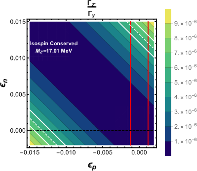
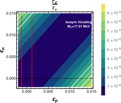
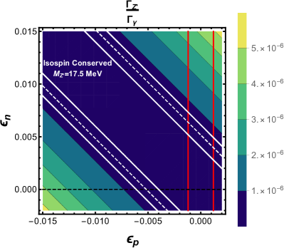
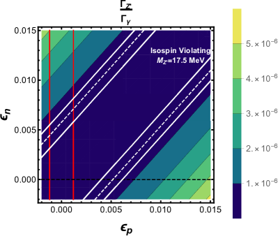
Figure 2: On the left (right) panels, contour plots of the ratio $\Gamma_{Z^{\prime}}/\Gamma_{\gamma}$ (see Eq. (53) for the isospin conserving (violating) limit. The white dashed and solid lines correspond to the best fit and to the 1$\sigma$ interval for the experimental best fit values for $\Gamma_{Z^{\prime}}/\Gamma_{\gamma}$, under the assumption BR$(Z^{\prime}\to e^{+}e^{-})=1$. The region between the two red vertical lines corresponds to the viable protophobic region of the parameter space, as allowed by NA48/2 constraints, while the horizontal dashed line corresponds to the pure dark photon limit. On both upper panels we have taken $m_{Z^{\prime}}$=17.01 MeV, as well as the experimental best fit value $\Gamma_{Z^{\prime}}/\Gamma_{\gamma}=6(1)\times 10^{-6}$ (following the fit values reported in [44]). The lower panels illustrate the case in which $m_{Z^{\prime}}$=17.5 MeV, for an experimental best fit value $\Gamma_{Z^{\prime}}/\Gamma_{\gamma}=0.5(0.2)\times 10^{-6}$, in agreement with the values quoted in [55] (for which we have taken a conservative estimate of the error in $\Gamma_{Z^{\prime}}/\Gamma_{\gamma}\sim 0.2\times 10^{-6}$, following the uncertainties of [44]).

Isospin breaking

In the above discussion it has been implicitly assumed that the ⁸Be states have a well-defined isospin; however, as extensively noted in the literature [140, 141, 142, 143, 144], the ⁸Be states are in fact isospin-mixed. In order to take the latter effects into account, isospin breaking in the electromagnetic transition operators arising from the neutron–proton mass difference was studied in detail in Ref. [55], and found to have potentially serious implications for the quark-level couplings required to explain the ⁸Be signal. In what follows we summarise the most relevant points, which will be included in the present study

For a doublet of spin $J$, the physical states (with superscripts $s_{1}$ and $s_{2}$) can be defined as [144]

$$\Psi_{J}^{s_{1}}\,=\,\alpha_{J}\,\Psi_{J,T=0}\,+\,\beta_{J}\,\Psi_{J,T=1}\,,\quad\quad\Psi_{J}^{s_{2}}\,=\,\beta_{J}\,\Psi_{J,T=0}\,-\,\alpha_{J}\,\Psi_{J,T=1}\,,$$ (62)

in which the relevant mixing parameters $\alpha_{J}$ and $\beta_{J}$ can be obtained by computing the widths of the isospin-pure states using the Quantum Monte Carlo (QMC) approach [144]. As pointed out in [55], this procedure may be used for the electromagnetic transitions of isospin-mixed states as well. However, the discrepancies with respect to the experimental results are substantial, even after including the meson-exchange currents in the relevant matrix element [144]. To address this deficiency, an isospin breaking effect was introduced in the hadronic form factor of the electromagnetic transition operators themselves in Ref. [55] (following [145, 146]). This has led to changes in the relative strength of the isoscalar and isovector transition operators which appear as a result of isospin-breaking in the masses of isospin multiplet states, e.g. the nonzero neutron-proton mass difference. The isospin-breaking contributions have been incorporated through the introduction of a spurion, which regulates the isospin-breaking effects within an isospin-invariant framework through a “leakage” parameter (controlled by non-perturbative effects). The “leakage” parameter is subsequently determined by matching the resulting $M1$ transition rate of the 17.64 MeV decay of ⁸Be with its experimental value, using the matrix elements of Ref. [144]. This prescription leads to the corrected ratio of partial widths [55],

$$\frac{\Gamma(^{8}\text{Be}^{*}\rightarrow{{}^{8}\text{Be}}+Z^{\prime})}{\Gamma(^{8}\text{Be}^{*}\rightarrow{{}^{8}\text{Be}}+\gamma)}=|0.05\,(\varepsilon^{V}_{p}+\varepsilon^{V}_{n})+0.95\,(\varepsilon^{V}_{p}-\varepsilon^{V}_{n})|^{2}\left[1-\left(\frac{m_{Z^{\prime}}}{18.15\text{ MeV}}\right)^{2}\right]^{3/2}\,,$$ (63)

and consequently, to new bounds on the relevant quark (nucleon) couplings necessary to explain the anomalous IPC in ⁸Be. On the upper right panel of Fig. 2, we display the isospin-violating scenario of Eq. (63), in the $\varepsilon_{p}$ vs. $\varepsilon_{n}$ plane, for $m_{Z^{\prime}}$=17.01 MeV and for the experimental best fit value $\Gamma_{Z^{\prime}}/\Gamma_{\gamma}=6(1)\times 10^{-6}$ [44]. A comparison with the case of isospin conservation (upper left plot) reveals a $15\%$ modification with respect to the allowed protophobic range of $\varepsilon_{n}$ in the isospin violating case.

Other than the best fit values for the mass of the mediator and normalised branching fraction for the predominantly isosinglet ⁸Be excited state with an excitation energy 18.15 MeV (here denoted as ${}^{8}\text{Be}^{*}$), it is important to take into account the IPC null results for the predominantly isotriplet excited state (${}^{8}\text{Be}^{*^{\prime}}$), as emphasised in [47]. In particular, in the presence of a finite isospin mixing, the latter IPC null result would call for a kinematic suppression, thus implying a larger preferred mass for the $Z^{\prime}$, in turn leading to a large phase space suppression. This may translate into (further) significant changes for the preferred quark (nucleon) couplings to the $Z^{\prime}$ (corresponding to a heavier $Z^{\prime}$, and to significantly smaller normalised branching fractions when compared to the preferred fit reported in [48]). Considering the benchmark value $\Gamma_{Z^{\prime}}/\Gamma_{\gamma}=0.5\times 10^{-6}$ [55], we obtain the following constraint in the isospin conserving limit,

$$|\varepsilon^{V}_{p}+\varepsilon^{V}_{n}|\approx\frac{(3-6)\times 10^{-3}}{\sqrt{\text{BR}(Z^{\prime}\to e^{+}e^{-})}}\,.$$ (64)

Leading to the above limits, we have used a conservative estimate for the error in $\Gamma_{Z^{\prime}}/\Gamma_{\gamma}$ ($\sim 0.2\times 10^{-6}$) following the quoted uncertainties in [44]. In Fig. 2, the bottom panels illustrate the relevant parameter space for the isospin conserving and isospin violating limits (respectively left and right plots).

To summarise, it is clearly important to further improve the estimation of nuclear isospin violation, and perform more accurate fits for the null result of IPC in ${}^{8}\text{Be}^{*^{\prime}}$ (in addition to the currently available fits for the predominantly isosinglet ⁸Be excited state). This will allow determining the ranges for the bounds on the relevant quark (nucleon) couplings of the $Z^{\prime}$ necessary to explain the anomalous IPC in ⁸Be. However, in view of the guesstimates discussed here, in our numerical analysis we will adopt conservative ranges for different couplings (always under the assumption $\text{BR}(Z^{\prime}\to e^{+}e^{-})=1$),

$$|\varepsilon^{V}_{n}| \;=\; (2-15)\times 10^{-3}\,,$$ (65)

$$|\varepsilon^{V}_{p}| \;\lesssim\; 1.2\times 10^{-3}\,.$$ (66)

5 Phenomenological constraints on neutral (vector and axial) couplings

If, and as discussed in the previous section, the new couplings of fermions to the light $Z^{\prime}$ must satisfy several requirements to explain the anomalous IPC in ⁸Be, there are extensive constraints arising from various experiments, both regarding leptonic and hadronic couplings. In this section, we collect the most important ones, casting them in a model-independent way, and subsequently summarising the results of the new fit carried for the case of light Majorana neutrinos (which is the case in the model under consideration).

5.1 Experimental constraints on a light $\boldsymbol{Z^{\prime}}$ boson

The most relevant constraints arise from negative $Z^{\prime}$ searches in beam dump experiments, dark photon bremsstrahlung and production, parity violation, and neutrino-electron scattering.

Searches for $\boldsymbol{Z^{\prime}}$ in electron beam dump experiments

The non-observation of a $Z^{\prime}$ in experiments such as SLAC E141, Orsay and NA64 [147], as well as searches for dark photon bremsstrahlung from electron and nuclei scattering, can be interpreted in a two-fold way: (i) absence of $Z^{\prime}$ production due to excessively feeble couplings; (ii) excessively rapid $Z^{\prime}$ decay, occurring even prior to the dump. Under assumption (i) (i.e. negligible production), one finds the following bounds

$${\varepsilon^{V}_{ee}}^{2}+{\varepsilon^{A}_{ee}}^{2}<1.1\times 10^{-16}\,,$$ (67)

while (ii) (corresponding to fast decay) leads to

$$\sqrt{{|\varepsilon^{V}_{ee}|}^{2}+{|\varepsilon^{A}_{ee}|}^{2}}\gtrsim 4\times 10^{-4}\>\sqrt{\text{BR}(Z^{\prime}\to e^{+}e^{-})}\,.$$ (68)

Searches for dark photon production

A bound can also be obtained from the KLOE-2 experiment, which has searched for $e^{+}e^{-}\to X\gamma$, followed by the decay $X\to e^{+}e^{-}$ [148], leading to

$${\varepsilon^{V}_{ee}}^{2}+{\varepsilon^{A}_{ee}}^{2}<\frac{4\times 10^{-6}}{{\text{BR}(Z^{\prime}\to e^{+}e^{-})}}\,.$$ (69)

Similar searches were also performed at BaBar, although the latter were only sensitive to slightly heavier candidates, with masses $m_{X}>20$ MeV [149].

Light meson decays

In addition to the (direct) requirements that an explanation of the ⁸Be anomaly imposes on the couplings of the $Z^{\prime}$ to quarks - already discussed in Section 4-, important constraints on the latter arise from several light meson decay experiments. For instance, this is the case of searches for $\pi^{0}\to\gamma Z^{\prime}(Z^{\prime}\to ee)$ and $K^{+}\to\pi^{+}Z^{\prime}(Z^{\prime}\to ee)$ at the NA48/2 [139] experiment, as well as searches for $\phi^{+}\to\eta^{+}Z^{\prime}(Z^{\prime}\to ee)$ at KLOE-2 [148]. Currently, the most stringent constraint does arise from the rare pion decays searches which lead, for $m_{Z^{\prime}}\simeq 17$ MeV [139], to the following bound

$$|2\varepsilon^{V}_{uu}+\varepsilon^{V}_{dd}|\,=\,|\varepsilon^{V}_{p}|\,\lesssim\,\frac{1.2\times 10^{-3}}{\sqrt{\textrm{BR}(Z^{\prime}\to e^{+}e^{-})}}\,.$$ (70)

If one confronts the range for $|\varepsilon^{V}_{p}+\varepsilon^{V}_{n}|$ required to explain the anomalous IPC in ⁸Be (see Eq. (64)), with the comparatively small allowed regime for $|\varepsilon^{V}_{p}|$ from the above equation, it is clear that in order to explain the anomaly in ⁸Be the neutron coupling $\varepsilon^{V}_{n}$ must be sizeable (This enhancement of neutron couplings (or suppression of the proton ones) is also often referred to as a “protophobic scenario” in the literature). Further (subdominant) bounds can also be obtained from neutron-lead scattering, proton fixed target experiments and other hadron decays, but we will not take them into account in the present study

Constraints arising from parity-violating experiments

Very important constraints on the product of vector and axial couplings of the $Z^{\prime}$ to electrons arise from the parity-violating Møller scattering, measured at the SLAC E158 experiment [150]. For $m_{Z^{\prime}}\simeq 17$ MeV, it yields [99]

$$|\varepsilon^{V}_{ee}\varepsilon^{A}_{ee}|\lesssim 1.1\times 10^{-7}.$$ (71)

Further useful constraints on a light $Z^{\prime}$ couplings can be inferred from atomic parity violation in Caesium, in particular from the measurement of the effective weak charge of the Cs atom [151, 152]. At the $2\sigma$ level [153], these yield

$$|\Delta Q_{w}|\,=\,|\frac{2\sqrt{2}}{G_{F}}\,4\pi\alpha\,\varepsilon^{A}_{ee}\left[\varepsilon^{V}_{uu}(2Z+N)+\varepsilon^{V}_{dd}(Z+2N)\right]\left(\frac{\mathcal{K}(m_{Z^{\prime}})}{m_{Z^{\prime}}^{2}}\right)|\,\lesssim\,0.71\,,$$ (72)

in which $\mathcal{K}$ is an atomic form factor, with $\mathcal{K}(17\,\mathrm{MeV})\simeq 0.8$ [152]. For the anomalous IPC favoured values of $\varepsilon^{V}_{uu(dd)}$, the effective weak charge of the Cs atom measurement provides a very strong constraint on $|\varepsilon^{A}_{ee}|$, $|\varepsilon^{A}_{ee}|\lesssim 2.6\times 10^{-9}$, which is particularly relevant for our scenario, as it renders a combined explanation of $(g-2)_{e}$ and the anomalous IPC particularly challenging. As we will subsequently discuss, the constraints on $|\varepsilon^{A}_{ee}|$ exclude a large region of the parameter space, leading to a “predictive” scenario for the $Z^{\prime}$ couplings.

Neutrino-electron scattering experiments

Finally, neutrino–electron scattering provides stringent constraints on the $Z^{\prime}$ neutrino couplings [155, 156, 154], with the tightest bounds arising from the TEXONO and CHARM-II experiments. In particular, for the mass range $m_{Z^{\prime}}\simeq 17\>\mathrm{MeV}$, the most stringent bounds are in general due to the TEXONO experiment [119]. While for some simple $Z^{\prime}$ constructions the couplings are flavour-universal, the extra fermion content in our model leads to a decoupling of the lepton families in such a way that only the couplings to electron neutrinos can be constrained with the TEXONO data. For muon neutrinos, slightly weaker but nevertheless very relevant bounds can be obtained from the CHARM-II experiment [120].

5.2 Majorana neutrinos: fitting the leptonic axial and vector couplings

In the present model, neutrinos are Majorana particles, which implies that the corresponding flavour conserving pure vector part of the $Z^{\prime}$-couplings vanishes. The fits performed in Refs. [155, 156, 154] are thus not directly applicable to our study; consequently we have performed new two-dimensional fits to simultaneously constrain the axial couplings to electron and muon neutrinos, and the vector coupling to electrons, following the prescription of Ref. [154]. As argued earlier, the axial coupling to electrons has to be negligibly small in order to comply with constraints from atomic parity violation and, for practical purposes, these will henceforth be set to zero in our analyses.

In Fig. 3 we show the particular likelihood contours deviating $1$ and $2\,\sigma$ from the best fit point for the neutrino–electron scattering data, which is found to lie very close to the SM prediction. Applying the constraints on the electron vector coupling $\varepsilon^{V}_{ee}$ obtained from NA64 [147] and KLOE-2 [148] leads to the limits

$$|\varepsilon_{\nu_{e}\nu_{e}}^{A}| \lesssim 1.2\times 10^{-5}\,\text{,}$$

$$|\varepsilon_{\nu_{\mu}\nu_{\mu}}^{A}| \lesssim 12.2\times 10^{-5}\,\text{,}$$ (73)

leading to which we have assumed the smallest allowed electron coupling $|\varepsilon_{ee}^{V}|\sim 4\times 10^{-4}$. Note that interference effects between the charged and neutral currents (as discussed in Refs. [55, 155, 156, 154]) do not play an important role in this scenario, due to vanishing neutrino vector couplings. The technical details regarding the calculation and fitting procedure referred to above can be found in the Appendix.

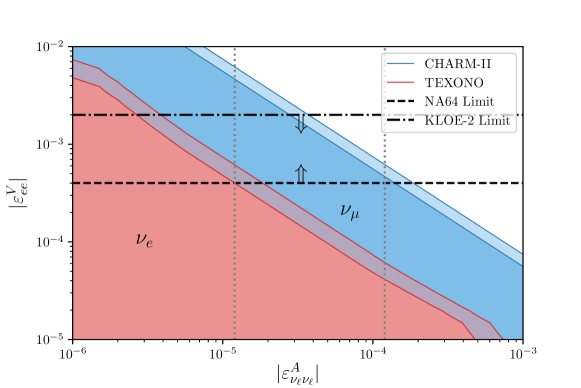
Figure 3: New $\chi^{2}$-fit of the $\bar{\nu}_{e}\>e$ scattering data of TEXONO (red) and the $\bar{\nu}_{\mu}\>e$ scattering data of CHARM-II (blue), displaying the 1- and 2-$\sigma$ allowed regions around the best fit point (respectively darker and lighter colours). The lower bound of NA64 (dashed line) and the upper bound by KLOE-2 (dash-dotted line) are also shown, with the arrows identifying the viable allowed regions. The obtained upper limits on the axial coupling to neutrinos, cf. Eq (73), are marked by dotted lines: the TEXONO data mostly constrains the couplings to electron neutrinos while the CHARM-II data is responsible for the constraints on the couplings to muon neutrinos.

To conclude this section, we list below a summary of the relevant constraints so far inferred on the couplings of the $Z^{\prime}$ to matter: combining the required ranges of couplings needed to explain the anomalous IPC signal with the relevant bounds from other experiments, we have established the following ranges for the couplings (assuming $\text{BR}(Z^{\prime}\to e^{+}e^{-})=1$),

$$2\times 10^{-3}\;\lesssim\;|\varepsilon^{V}_{n}| \;\lesssim\; 15\times 10^{-3}\,,$$ (74)

$$|\varepsilon^{V}_{p}| \;\lesssim\; 1.2\times 10^{-3}\,,$$ (75)

$$0.4\times 10^{-3}\;\lesssim\;|\varepsilon^{V}_{ee}| \;\lesssim\; 2\times 10^{-3}\,,$$ (76)

$$|\varepsilon^{A}_{ee}| \;\lesssim\; 2.6\times 10^{-9}\,,$$ (77)

$$|\varepsilon^{A}_{\nu_{e}\nu_{e}}| \lesssim 1.2\times 10^{-5}\,,$$ (78)

$$|\varepsilon^{A}_{\nu_{\mu}\nu_{\mu}}| \lesssim 12.2\times 10^{-5}\,.$$ (79)

6 Addressing the anomalous IPC in ⁸Be: impact for a combined explanation of $\boldsymbol{(g-2)_{e,\mu}}$

As a first step, we apply the previously obtained model-independent constraints on the $Z^{\prime}$ couplings to the specific structure of the present model. After taking the results of (negative) collider searches for the exotic matter fields into account, we will be able to infer an extremely tight range for $\varepsilon$ (which we recall to correspond to a redefinition of the effective kinetic mixing parameter, cf. Eq. (19)). In turn, this will imply that very little freedom is left to explain the experimental discrepancies in the light charged lepton anomalous magnetic moments, the latter requiring an interplay of the $h_{\ell\ell}$ and $k_{\ell\ell}$ couplings.

6.1 Constraining the model’s parameters

The primary requirements to explain the anomalous IPC in ⁸Be concern the physical mass of the $Z^{\prime}$, which should approximately be

$$m_{Z^{\prime}}\,\approx 17\,\mathrm{MeV}\,,$$ (80)

and the strength of its couplings to nucleons (protons and neutrons), as given in Eqs. (65, 66). With $\varepsilon^{V}_{qq}$ as defined in Eq. (33), and recalling that $\varepsilon_{p}=2\,\varepsilon^{V}_{uu}+\varepsilon^{V}_{dd}$ and $\varepsilon_{n}=\varepsilon^{V}_{uu}+2\,\varepsilon^{V}_{dd}$, one obtains the following constraints on $\varepsilon_{B-L}$ and $\varepsilon$

$$|\varepsilon_{n}^{V}| = |\varepsilon_{B-L}|\,=\,(2-15)\times 10^{-3}\,,$$ (81)

$$|\varepsilon_{p}^{V}| = |\varepsilon+\varepsilon_{B-L}|\lesssim 1.2\times 10^{-3}\,.$$ (82)

Furthermore, this implies an upper bound for the VEV of $h_{X}$, $v_{X}\lesssim 14\>\mathrm{GeV}$, since

$$m_{Z^{\prime}}\approx m_{B^{\prime}}\,=\,2\,e\,|\varepsilon_{B-L}|\,v_{X}\,.$$ (83)

In the absence of heavy vector-like leptons, there are no other sources of mixing in the lepton section in addition to the PMNS. This would imply that the effective couplings of the $Z^{\prime}$ to neutrinos are identical to that of the neutron (up to a global sign), that is

$$\varepsilon_{\nu\nu}^{A}\,=\,\varepsilon_{B-L}\,,$$ (84)

which, in view of Eq. (81), leads to $\varepsilon_{\nu\nu}^{A}=(2-10)\times 10^{-3}$. However, the bounds of the TEXONO experiment [119] for neutrino-electron scattering (cf. Eq. (5.2)) imply that for the minimal allowed electron coupling $|\varepsilon_{ee}^{V}|\gtrsim 0.4\times 10^{-3}$ one requires

$$|\varepsilon_{\nu\nu}^{A}|\,\lesssim\,1.2\,(12.2)\,\times\,10^{-5}\,,$$ (85)

for electron (muon) neutrinos. As can be inferred, this is in clear conflict with the values of $\varepsilon_{\nu\nu}^{A}$ required to explain the ⁸Be anomalous IPC, which are $\mathcal{O}(10^{-3})$.

In order to circumvent this problem, the effective $Z^{\prime}$ coupling to the SM-like neutrinos must be suppressed. The additional vector-like leptons open the possibility of having new sources of mixing between the distinct species of neutral leptons; the effective neutrino coupling derived in Section 2.3 allows to suppress the couplings by a factor $\sim(1-{\lambda_{L\,\alpha}^{2}v_{X}^{2}/M_{L\,\alpha}^{2}})$ (see Eq. (39), with $\alpha$ denoting SM flavours), hence implying

$$|1-\frac{\lambda_{L}^{2}v_{X}^{2}}{M_{L}^{2}}|\,\lesssim 0.01\,.$$ (86)

Thus, up to a very good approximation, we can assume $\lambda_{L}v_{X}\simeq M_{L}$ for each lepton generation $\alpha$. On the other hand, from Eqs. (36) and (72) it follows that the bound from atomic parity violation in Caesium tightly constrains the isosinglet vector-like lepton coupling $\lambda_{E}$ (for the first lepton generation), leading to

$$|\varepsilon_{ee}^{A}|\,=\,\left|\frac{1}{2}\left(\frac{\lambda_{E}^{2}\,v_{X}^{2}}{M_{E}^{2}}-\frac{\lambda_{L}^{2}\,v_{X}^{2}}{M_{L}^{2}}\right)\varepsilon_{B-L}\right|\,\lesssim\,2.6\times 10^{-9}\,\text{,}$$ (87)

which in turn implies

$$\left|\frac{\lambda_{E}^{2}\,v_{X}^{2}}{M_{E}^{2}}-\frac{\lambda_{L}^{2}\,v_{X}^{2}}{M_{L}^{2}}\right|\,\lesssim 2.6\times 10^{-6}\,\text{.}$$ (88)

Notice that this leads to a tight correlation between the isosinglet and isodoublet vector-like lepton couplings, $\lambda_{E}$ and $\lambda_{L}$, respectively. More importantly, the above discussion renders manifest the necessity of having the additional field content (a minimum of two generations of heavy vector-like leptons).

Together with Eqs. (40) and (41), Eqs. (86) and (88) suggest that the $Z^{\prime}$ coupling to electrons is now almost solely determined by $\varepsilon$. In particular, the KLOE-2 [148] limit of Eq. (69) for $\varepsilon_{ee}$ now implies

$$|\varepsilon|\,<\,0.002\,.$$ (89)

Further important constraints on the model’s parameters arise from the masses of the vector-like leptons, which are bounded from both below and above. On the one hand, the perturbativity limit of the couplings $\lambda_{L}$ and $\lambda_{E}$ implies an upper bound on the vector-like lepton masses. On the other hand, direct searches for vector-like leptons exclude vector-like lepton masses below $\sim 100\,\mathrm{GeV}$ [157] (under the assumption these dominantly decay into $W\nu$ pairs). This bound can be relaxed if other decay modes exist, for instance involving the $Z^{\prime}$ and $h_{X}$ as is the case in our scenario. However, and given the similar decay and production mechanisms, a more interesting possibility is to recast the results of LHC dedicated searches for sleptons (decaying into a neutralino and a charged SM lepton) for the case of vector-like leptons decaying into $h_{X}$ and a charged SM lepton. Taking into account the fact that the vector-like lepton’s cross section is a few times larger than the selectron’s or smuon’s [55, 158], one can roughly estimate that vector-like leptons with a mass $\sim 100\,\mathrm{GeV}$ can decay into a charged lepton and an $h_{X}$ with mass $\sim~{}(50-70)\,\mathrm{GeV}$. Therefore, as a benchmark choice we fix the tree-level mass of the vector-like leptons of all generations to $M_{L}=M_{E}=90\,\mathrm{GeV}$ (which yields a physical mass $\sim 110\,\mathrm{GeV}$, once the corrections due to mixing effects are taken into account). In turn, this implies that the couplings $\lambda_{L,E}$ should be sizeable $\lambda_{E}^{e}\approx\lambda_{L}^{e}\sim 6.4$ (for the first generation, due to the very stringent parity violation constraints), while for the second generation one only has $\lambda_{L}^{\mu}\sim 6.4$. (We notice that smaller couplings, still complying with all imposed constraints can still be accommodated, at the price of extending the particle content to include additional exotic fermion states.) In agreement with the the above discussion, we further choose $m_{h_{X}}=70\,\mathrm{GeV}$ as a benchmark value. Since $h_{X}$ can also decay into two right handed neutrinos (modulo a substantially large Majorana coupling $y_{M}$), leading to a signature strongly resembling that of slepton pair production, current negative search results then lead to constraints on $\varepsilon_{B-L}$. For the choice $m_{h_{X}}=70\,\mathrm{GeV}$, $\varepsilon_{B-L}$ should be close to its smallest allowed value $\varepsilon_{B-L}=0.002$  [55], which in turn implies the following range for $\varepsilon$

$$-0.0032\,\lesssim\,\varepsilon\,\lesssim\,-0.0008\,.$$ (90)

The combination of the previous constraint with the one inferred from the KLOE-2 limit on the couplings of the $Z^{\prime}$ to electrons, see Eq. (89), allows to derive the viability range for $\varepsilon$,

$$-0.002\,\lesssim\,\varepsilon\,\lesssim\,-0.0008\,.$$ (91)

Before finally addressing the feasibility of a combined explanation to the atomic ⁸Be and $(g-2)_{e,\mu}$ anomalies, let us notice that in the study of Ref. [159] the authors have derived significantly stronger new constraints on the parameter space of new (light) vector states, $X$, arising in $U(1)_{X}$ extensions of the SM, such as $U(1)_{B-L}$ models. The new bounds can potentially disfavour some well-motivated constructions, among which some aiming at addressing the ⁸Be anomalies, and arise in general from an energy-enhanced emission (production) of the longitudinal component ($X_{L}$) via anomalous couplings. We notice that the prototype model here investigated departs in several points from the assumptions of [159]. In the present $U(1)_{B-L}$ extension the heavy vector-like fermions do not contribute to anomaly cancellation, as the SM field content and three generations of right handed neutrinos (and independently, all the vector-like fermions) constitute a completely anomaly-free set under the extended gauge group. Moreover, there are no neutral vertices explicitly breaking $SU(2)_{L}$ – as can be seen from Eqs. (39) and (40), thus avoiding the potential constraints inferred for a possible energy-enhanced longitudinal emission of $X$.

6.2 A combined explanation of $\boldsymbol{(g-2)_{e,\mu}}$

In view of the stringent constraints on the parameter space of the model, imposed both from phenomenological arguments and from a satisfactory explanation of the anomalous IPC in ⁸Be, one must now consider whether it is still possible to account for the observed tensions in the electron and muon anomalous magnetic moments. As discussed both in the Introduction and in Section 3, the discrepancies between SM prediction and experimental observation have an opposite sign for electrons and muons, and exhibit a scaling behaviour very different from the naïve expectation (powers of the lepton mass ratio).

Given the necessarily small mass of the $Z^{\prime}$ and the large couplings between SM leptons and the heavier vector-like states ($\lambda_{L,E}$), in most of the parameter space the new contributions to $(g-2)_{e,\mu}$ are considerably larger than what is suggested from experimental data. Firstly, recall that due to the opposite sign of the loop functions for (axial) vector and (pseudo)scalar contributions, a cancellation between the latter contributions allows for an overall suppression of each $(g-2)_{e,\mu}$. Moreover, a partial cancellation between the distinct diagrams can lead to $\Delta a_{\mu}$ and $\Delta a_{e}$ with opposite signs; this requires nevertheless a large axial coupling to electrons, which is experimentally excluded. However, an asymmetry in the couplings of the SM charged leptons to the vector-like states belonging to the same generation can overcome the problem, generating a sizeable “effective” axial coefficient $g_{A}^{\ell\ell}$: while for electrons Eq. (88) implies a strong relation between $\lambda_{L}$ and $\lambda_{E}$, the (small) couplings $h_{\ell}$ and $k_{\ell}$ remain essentially unconstrained and can induce such an asymmetry, indeed leading to the desired ranges for the anomalous magnetic moments.

This interplay of the different (new) contributions can be understood from Fig. 4, which illustrates the $h_{X}$ and the $Z^{\prime}$ contributions to the electron and muon $|\Delta a_{\ell}|$, as a function of the $h_{\ell}$ coupling for $\ell=e$ (left) and $\ell=\mu$ (right). The $h_{X}$-induced contribution to $(g-2)_{\ell}$ changes sign when the pseudoscalar dominates over the scalar contribution (for the choices of the relevant Yukawa couplings $h_{\ell}$ and $k_{\ell}$). Likewise, a similar effect occurs for the $Z^{\prime}$ contribution when the axial-vector contribution dominates over the vector one. The transition between positive (solid line) and negative (dashed line) contributions - from $Z^{\prime}$ (orange), $h_{X}$ (green) and combined (blue) - is illustrated by the sharp kinks visible in the logarithmic plots of Fig. 4. In particular, notice that the negative electron $\Delta a_{e}$ is successfully induced by the flip of the sign of the $h_{X}$ contribution, while a small positive muon $\Delta a_{\mu}$ arises from the cancellation of the scalar and the $Z^{\prime}$ contributions. Leading to the numerical results of Fig. 4 (and in the remaining of our numerical analysis), we have taken as benchmark values $\varepsilon_{B-L}=2\times 10^{-3}$ and $\varepsilon=-8\times 10^{-4}$ (which are consistent with the criterion for explaining the anomalous IPC in ⁸Be and respect all other imposed constraints). We emphasise that as a consequence of their already extremely constrained ranges, both the $B-L$ gauge coupling and the kinetic mixing parameter have a very minor influence on the contributions to the anomalous magnetic lepton moments (when varied in the allowed ranges). Furthermore, the masses $M_{L,E}$ and $m_{h_{X}}$ can be slightly varied with respect to the proposed benchmark values, with only a minor impact on the results; a mass-splitting between $M_{E}$ and $M_{L}$ (for each generation) slightly modifies the slope of the curves presented in Fig. 5, while an overall scaling to increase $M_{L,E}$ would imply taking (even) larger values for most of the couplings in their allowed regions. (Notice however that the model’s parameter space is severely constrained, so that any departure from the benchmark values is only viable for a comparatively narrow band in the parameter space.)

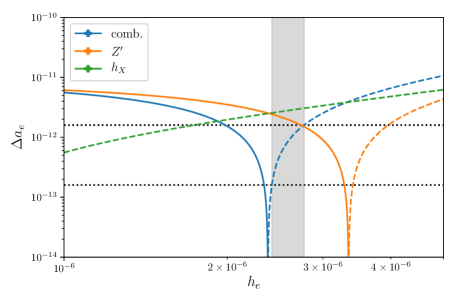
Figure 4: Contributions to the anomalous magnetic moment of charged leptons, $|\Delta a_{\ell}|$, as a function of the $h_{\ell}$ coupling for $\ell=e$ (left) and $\ell=\mu$ (right). Solid (dashed) lines correspond to positive (negative) values of $\Delta a_{\ell}$; the colour code denotes contributions from the $Z^{\prime}$ (orange) and from $h_{X}$ (green), as well as the combined one (blue). Horizontal (dotted) lines denote the $2\sigma$ and $3\sigma$ regions of the electron and muon $\Delta a_{\ell}$. A vertical opaque region corresponds to the $h_{\ell}$ interval for which the combined contributions to $\Delta a_{e(\mu)}$ lie within the $2\sigma$ ($3\sigma$) region. Leading to this figure, we have selected a benchmark choice of parameters complying with all the constraints mentioned in Section 5: $M_{L}=M_{E}=90\,\mathrm{GeV}$, $\lambda_{E}=\lambda_{L}=M_{L}/v_{X}$, $m_{h_{X}}=70\,\mathrm{GeV}$, $\varepsilon=-8\times 10^{-4}$, $\varepsilon_{B-L}=0.002$ and $k_{\ell}=10^{-7}$.

To conclude the discussion, and provide a final illustration of how constrained the parameter space of this simple model becomes, we display in Fig. 5 the regions complying at the $2\sigma$ level with the observation of $(g-2)_{\ell}$ in the planes spanned by $h_{\ell}$ and $k_{\ell}$ (for $\ell=e,\mu$). The colour code reflects the size of the corresponding entry of $\lambda_{E}^{\ell}$, which is varied in the interval $[1,8]$ (recall that for the electron anomalous magnetic moment, $\lambda_{L}^{e}=\lambda_{E}^{e}\sim 6.4$). All remaining parameters are fixed to the same values used for the numerical analysis leading to Fig. 4.

Notice that, as mentioned in the discussion at the beginning of the section (cf. 6.1), the extremely stringent constraints on the $Z^{\prime}$ couplings arising from atomic parity violation and electron neutrino scatterings render the model essentially predictive in what concerns $(g-2)_{e}$: only the narrow black band of the $(h_{e}-k_{e})$ space succeeds in complying with all available constraints, while both addressing the IPC ⁸Be anomaly, and saturating the current discrepancy between SM and observation on $(g-2)_{e}$. For the muons, and although $h_{\mu}$ remains strongly correlated with $k_{\mu}$, the comparatively larger freedom associated with $\lambda_{E}^{\mu}$ (recall that no particular relation between $\lambda_{L}$ and $\lambda_{E}$ is required by experimental data) allows to identify a wider band in $(h_{\mu}-k_{\mu})$ space for which $\Delta a_{\mu}$ is satisfied at $2\sigma$.

Finally, notice that the $h_{\ell}$ and $k_{\ell}$ are forced into a strongly hierarchical pattern, at least in what concerns the first two generations.

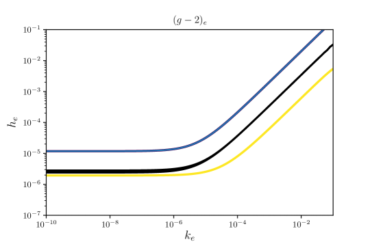
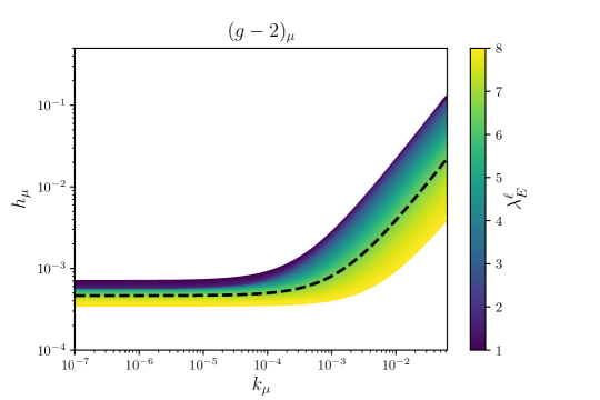
Figure 5: Viable regions in $h_{\ell}$ vs. $k_{\ell}$ parameter space: on the left (right) $\ell=e\,(\mu)$). In both panels the colour code denotes the value of $\lambda_{E}^{\ell}$ ($\lambda_{E}=1-8$, from dark violet to yellow). On the left panel, only the central black line complies with $(g-2)_{e}$ at the $2\sigma$ level (i.e. $\lambda_{E}^{e}\sim 6.4$); for the right panel, all the coloured region allows to satisfy $(g-2)_{\mu}$ at $2\sigma$ (the dashed black line illustrates the value $\lambda_{E}^{\mu}\sim 6.4$). All other relevant parameters fixed as leading to Fig. 4.

7 Concluding remarks

Despite the absence of a direct discovery of new resonances at high energy colliders, several low-energy observables exhibit tensions with SM predictions, to various degrees of significance and longevity. The discrepancy between the SM prediction and experimental observation regarding the anomalous magnetic moment of the muon is perhaps the most longstanding anomaly, currently exhibiting a tension around $3.3\sigma$; more recently, the electron $(g-2)$ also started to display tensions between theory and observation (around $2.5\sigma$), all the most intriguing since instead of following a naïve scaling proportional to powers of the light lepton masses, the comparison of $\Delta a_{e,\mu}$ suggests the presence of a New Physics which violates lepton flavour universality. In recent years, an anomalous angular correlation was observed for the 18.15 MeV nuclear transition of ⁸Be atoms, in particular an enhancement of the IPC at large angles, with a similar anomaly having been observed in ⁴He transitions.

An interesting possibility is to interpret the atomic anomalies as being due to the presence of a light vector boson, with a mass close to $17$ MeV. Should such a state have non-vanishing electroweak couplings to the standard fields, it could also have an impact on $\Delta a_{e,\mu}$. In this work, we have investigated the phenomenological implications of a BSM construction in which the light vector boson arises from a minimal extension of the gauge group via an additional $U(1)_{B-L}$. Other than the scalar field (whose VEV is responsible for breaking the new $U(1)$), three generations of Majorana right-handed neutrinos, as well as of heavy vector-like leptons are added to the SM field content. As discussed here, the new matter fields play an instrumental role both in providing additional sources of leptonic mixing, and in circumventing the very stringent experimental constraints.

After having computed the modified couplings, and summarised the model’s contributions to the light charged lepton anomalous magnetic moments, we identified how addressing the anomalous IPC in ⁸Be constrained the couplings of matter to the new $Z^{\prime}$. Once all remaining phenomenological constraints are imposed on the model’s parameter space, one is led to an extremely tight scenario, in which saturating the (opposite-sign) tensions on $\Delta a_{e,\mu}$ can only be achieved via a cancellation of the new (pseudo)scalar and (axial)vector contributions.

The very stringent constraints arising from atomic parity violation lead to an extremely strong correlation for the new couplings $h_{e}$ and $k_{e}$ (first generation couplings of vector-like leptons to the SM Higgs) in order to comply with $(g-2)_{e}$; moreover, this requires a nearly non-perturbative regime for the $\ell-L-h_{X}$ couplings ($\lambda_{L,E}$). The situation is slightly less constraining for the muon anomalous magnetic moment, albeit leading to a non-negligible dependence of the corresponding couplings, $h_{\mu}$ and $k_{\mu}$.

Future measurements of right-handed neutral couplings, or axial couplings, for the second generation charged leptons could further constrain the new muon couplings. Although this clearly goes beyond the scope of the present work, one could possibly envisage parity-violation experiments carried in association with muonic atoms. As an example, in experiments designed to test parity non-conservation (PNC) with atomic radiative capture (ARC), the measurement of the forward-backward asymmetry of the photon radiated by muons ($2s\to 1s$ transition) is sensitive to (neutral) muon axial couplings [160]. Further possibilities include scattering experiments, such as MUSE at PSI [161], or studying the muon polarisation in $\eta$ decays (REDTOP experiment proposal [162]), which could allow a measurement of the axial couplings of muons.

Appendix

Electron-neutrino scattering data: analysis and fits

In this Appendix we detail the formalism used for the analysis of the available data on electron-neutrino scattering, upon which rely the constraints presented in Section 5.1. The data used arises from two different experimental set-ups, CHARM-II and TEXONO.

In general, the differential cross section for neutrino and antineutrino scattering can be easily computed [154]

$$\frac{d\sigma}{dT}(\bar{\nu}e^{-}\to\bar{\nu}e^{-}) =\frac{m_{e}}{4\,\pi}\left[G_{+}^{2}+G_{-}^{2}\left(1-\frac{T}{E_{\nu}}\right)^{2}-G_{+}G_{-}\frac{m_{e}\,T}{E_{\nu}^{2}}\right]\,\text{,}$$ (92)

$$\frac{d\sigma}{dT}(\nu e^{-}\to\nu e^{-}) =\frac{m_{e}}{4\,\pi}\left[G_{-}^{2}+G_{+}^{2}\left(1-\frac{T}{E_{\nu}}\right)^{2}-G_{+}G_{-}\frac{m_{e}\,T}{E_{\nu}^{2}}\right]\,\text{,}$$ (93)

where $T$ is the recoil energy of the electron and $E_{\nu}$ the energy of the (anti)neutrino. The coefficients $G_{\pm}$ are defined as

$$G_{\pm}\,=\,\sum_{i=W,Z,Z^{\prime}}\frac{1}{P_{i}}\,(g_{V_{i}}^{\nu\nu}-g_{A_{i}}^{\nu\nu})\,(g_{V_{i}}^{ee}\pm g_{A_{i}}^{ee})\,\text{.}$$ (94)

In the above, the sum runs over all relevant vector bosons (i.e. $W$, $Z$ and $Z^{\prime}$), with $P_{i}$ denoting the denominator of the corresponding propagators; $g_{V_{i}}$ and $g_{A_{i}}$ correspond to the vector and axial couplings of the involved vector bosons to (anti)neutrinos and electrons. Since the energy of the neutrinos is well below the masses of the relevant gauge bosons, we carry the following approximations

$$P_{W}\approx-\frac{\sqrt{2}\,g^{2}}{8\,G_{F}}\,\text{,}\quad P_{Z}\approx-\frac{\sqrt{2}\,g^{2}}{8\,G_{F}\,c_{w}^{2}}\,\text{,}\quad P_{Z^{\prime}}\sim-(2\,m_{e}\,T+m_{Z^{\prime}}^{2})\,\text{.}$$ (95)

For the case of the model under study, the vector and axial coefficients are given by

$$g_{V_{W}} = -g_{A_{W}}=\frac{g}{2\,\sqrt{2}}\quad\text{(for both $\nu$ and $e$),}$$ (96)

$$g_{A_{Z}}^{\nu\nu} = -\frac{g}{2\,c_{w}}\,\text{,}$$ (97)

$$g_{V_{Z}}^{ee} = -\frac{g\,(1-4\,s_{w}^{2})}{4\,c_{w}}\,\text{,}$$ (98)

$$g_{A_{Z}}^{ee} = \frac{g}{4\,c_{w}}\,\text{,}$$ (99)

$$g_{V_{Z^{\prime}}}^{ee} = e\varepsilon_{ee}^{V}\,\text{,}$$ (100)

$$g_{A_{Z^{\prime}}}^{\nu\nu} = 2\,e\,\varepsilon_{\nu\nu}^{A}\,\text{,}$$ (101)

with all other remaining coefficients vanishing. In order to take into account the fact that for Majorana neutrinos the $\nu$ and $\bar{\nu}$ final states are indistinguishable, a factor of 2 is present in the (axial) neutrino coefficients (effectively allowing to double the contributions from amplitudes involving two neutrino operators [163]).

Data from the CHARM-II experiment

To fit the data from the CHARM-II experiment (extracted from Table 2 of Ref. [120]), one can directly compare the differential cross-section, averaged over the binned recoil energy $T$, with the data. For neutrinos and antineutrinos, the average energies are $\braket{E_{\nu_{\mu}}}=23.7\,\mathrm{GeV}$ and $\braket{E_{\bar{\nu}_{\mu}}}=19.1\,\mathrm{GeV}$, respectively. Since no data correlation from the CHARM-II samples is available, we assume all data to follow a gaussian distribution, and accordingly define the $\chi^{2}$ function

$$\chi^{2}_{\text{CHARM-II}}\,=\,\sum_{i}\left(\frac{\sigma_{i}-\sigma_{i,\text{exp}}}{\Delta\sigma_{i,\text{exp}}}\right)^{2}\,\text{,}$$ (102)

where $i$ runs over the different bins. The $\chi^{2}$ is minimised, and its $1\sigma$ and $2\sigma$ contours around the minimum are computed.

Data from the TEXONO experiment

The analysis of the TEXONO data [119] is comparatively more involved than that of CHARM-II. Since TEXONO is a reactor experiment, the computation of the binned event rate requires knowledge of the reactor anti-neutrino flux. Following the approach of Ref. [154], the event rate can be computed as

$$R(T_{1},T_{2})\,=\,\frac{\rho_{e}}{T_{2}-T_{1}}\int\phi(E_{\bar{\nu}})\left[\int_{\bar{T}_{1}}^{\bar{T}_{2}}\frac{d\sigma}{dT}dT\right]dE_{\bar{\nu}}\,\text{,}$$ (103)

in which $T_{1,2}$ are the bin edges for the electron’s recoil energy, $\phi(E_{\bar{\nu}})$ is the neutrino flux, $\rho_{e}$ the electron density of the target material and $\bar{T}_{1,2}=\mathrm{min}(T_{1,2},T_{\text{max}})$; the maximum recoil energy $T_{\text{max}}$ can be defined as

$$T_{\text{max}}\,=\,\frac{2E_{\bar{\nu}}^{2}}{M+2\,E_{\bar{\nu}}}\,\text{.}$$ (104)

The (anti)neutrino flux is given by [164]

$$\phi(E_{\bar{\nu}})=\frac{1}{4\,\pi\,R^{2}}\frac{W_{\text{th}}}{\sum_{i}f_{i}E_{f,i}}\left(\sum_{i}f_{i}\rho_{i}(E_{\bar{\nu}})\right)\,\text{,}$$ (105)

in which the sums run over the reactor fuel constituents $i$; for each of the latter, $f_{i}$ is the fission rate, $E_{f,i}$ the fission energy and $\rho_{i}(E_{\bar{\nu}})$ the neutrino spectrum. The remaining intrinsic parameters are $W_{\text{th}}$ - the total thermal energy of the reactor, and $R$ which corresponds to the distance between reactor and detector (details of the reactor and general experimental set-up can be found in Ref. [165]). In what concerns the neutrino spectra, and depending on the different reactor fuel constituents, we use the fit of Ref. [166], in which spectra between $2-8\,\mathrm{MeV}$ are parametrised by the exponential of a fifth degree polynomial . (Lower energies are not relevant for our study, since the TEXONO data consists of 10 equidistant bins between $3-8\,\mathrm{MeV}$.)

We have thus obtained the electron density of the detector material $\rho_{e}$ of the TEXONO experiment by fitting the SM expectation of the binned event rate to the SM curve given in Fig. 16 of Ref. [119]. Our result is as follows

$$\rho_{e}\,\simeq\,2.77\times 10^{26}\>\mathrm{kg}^{-1}\,\text{.}$$ (106)

Finally, and to define the $\chi^{2}$ function for the TEXONO experiment data, we again rely on the experimental data Fig. 16 of Ref. [119], leading to

$$\chi^{2}_{\text{TEXONO}}\,=\,\sum_{i}\left(\frac{R_{i}-R_{i,\text{exp}}}{\Delta R_{i,\text{exp}}}\right)^{2}\,\text{,}$$ (107)

where $i$ counts the different bins in the recoil energy.

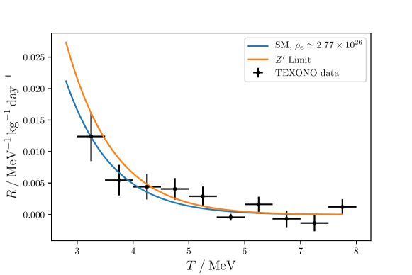
Figure 6: Data of the TEXONO experiment (neutrino rate $R$ in units of $\mathrm{MeV}^{-1}\,\mathrm{kg}^{-1}\,\mathrm{day}^{-1}$ as a function of the binned recoil energy $T$) [119], to which we superimpose our SM and $Z^{\prime}$ predictions, respectively corresponding to blue and orange lines.

In Fig. 6 we display the experimental data obtained by TEXONO, together with the (fitted) SM curve as well as the $Z^{\prime}$ prediction. Leading to the $Z^{\prime}$ curve we have taken the minimum couplings to electrons allowed by NA64 [147], and the maximum values of the couplings to neutrinos as derived from the TEXONO data [119]. The resulting fit is used in the analysis of Section 5.2, in particular in the results displayed in Fig. 3.

References

- [1] W. Ni, S. Pan, H. Yeh, L. Hou and J. Wan, Phys. Rev. Lett. 82 (1999), 2439-2442.
- [2] B. R. Heckel, C. Cramer, T. Cook, E. Adelberger, S. Schlamminger and U. Schmidt, Phys. Rev. Lett. 97 (2006), 021603 [arXiv:hep-ph/0606218 [hep-ph]].
- [3] S. Baessler, V. Nesvizhevsky, K. Protasov and A. Voronin, Phys. Rev. D 75 (2007), 075006 [arXiv:hep-ph/0610339 [hep-ph]].
- [4] G. Hammond, C. Speake, C. Trenkel and A. Pulido Paton, Phys. Rev. Lett. 98 (2007), 081101.
- [5] B. R. Heckel, E. Adelberger, C. Cramer, T. Cook, S. Schlamminger and U. Schmidt, Phys. Rev. D 78 (2008), 092006 [arXiv:0808.2673 [hep-ex]].
- [6] G. Vasilakis, J. Brown, T. Kornack and M. Romalis, Phys. Rev. Lett. 103 (2009), 261801 [arXiv:0809.4700 [physics.atom-ph]].
- [7] A. Serebrov, Phys. Lett. B 680 (2009), 423-427 [arXiv:0902.1056 [nucl-ex]].
- [8] V. Ignatovich and Y. Pokotilovski, Eur. Phys. J. C 64 (2009), 19-23.
- [9] A. Serebrov, O. Zimmer, P. Geltenbort, A. Fomin, S. Ivanov, E. Kolomensky, I. Krasnoshekova, M. Lasakov, V. Lobashev, A. Pirozhkov, V. Varlamov, A. Vasiliev, O. Zherebtsov, E. Aleksandrov, S. Dmitriev and N. Dovator, JETP Lett. 91 (2010), 6-10 [arXiv:0912.2175 [nucl-ex]].
- [10] S. Karshenboim, Phys. Rev. Lett. 104 (2010), 220406 [arXiv:1005.4859 [hep-ph]].
- [11] S. Karshenboim, Phys. Rev. D 82 (2010), 113013 [arXiv:1005.4868 [hep-ph]].
- [12] A. Petukhov, G. Pignol, D. Jullien and K. Andersen, Phys. Rev. Lett. 105 (2010), 170401 [arXiv:1009.3434 [physics.atom-ph]].
- [13] S. Karshenboim and V. Flambaum, Phys. Rev. A 84 (2011), 064502 [arXiv:1110.6259 [physics.atom-ph]].
- [14] S. Hoedl, F. Fleischer, E. Adelberger and B. Heckel, Phys. Rev. Lett. 106 (2011), 041801.
- [15] G. Raffelt, Phys. Rev. D 86 (2012), 015001 [arXiv:1205.1776 [hep-ph]].
- [16] H. Yan and W. Snow, Phys. Rev. Lett. 110 (2013) no.8, 082003 [arXiv:1211.6523 [nucl-ex]].
- [17] K. Tullney, F. Allmendinger, M. Burghoff, W. Heil, S. Karpuk, W. Kilian, S. Knappe-Gruneberg, W. Muller, U. Schmidt, A. Schnabel, F. Seifert, Y. Sobolev and L. Trahms, Phys. Rev. Lett. 111 (2013), 100801 [arXiv:1303.6612 [hep-ex]].
- [18] P. Chu, A. Dennis, C. Fu, H. Gao, R. Khatiwada, G. Laskaris, K. Li, E. Smith, W. Snow, H. Yan and W. Zheng, Phys. Rev. D 87 (2013) no.1, 011105 [arXiv:1211.2644 [nucl-ex]].
- [19] M. Bulatowicz, R. Griffith, M. Larsen, J. Mirijanian, T. Walker, C. Fu, E. Smith, W. Snow and H. Yan, Phys. Rev. Lett. 111 (2013), 102001 [arXiv:1301.5224 [physics.atom-ph]].
- [20] S. Mantry, M. Pitschmann and M. J. Ramsey-Musolf, Phys. Rev. D 90 (2014) no.5, 054016 [arXiv:1401.7339 [hep-ph]].
- [21] L. Hunter and D. Ang, Phys. Rev. Lett. 112 (2014) no.9, 091803 [arXiv:1306.1118 [hep-ph]].
- [22] E. Salumbides, W. Ubachs and V. Korobov, J. Molec. Spectrosc. 300 (2014), 65 [arXiv:1308.1711 [hep-ph]].
- [23] T. Leslie and J. Long, Phys. Rev. D 89 (2014) no.11, 114022 [arXiv:1401.6730 [hep-ph]].
- [24] A. Arvanitaki and A. A. Geraci, Phys. Rev. Lett. 113 (2014) no.16, 161801 [arXiv:1403.1290 [hep-ph]].
- [25] Y. Stadnik and V. Flambaum, Eur. Phys. J. C 75 (2015) no.3, 110 [arXiv:1408.2184 [hep-ph]].
- [26] S. Afach et al Phys. Lett. B 745 (2015), 58-63 [arXiv:1412.3679 [hep-ex]].
- [27] W. Terrano, E. Adelberger, J. Lee and B. Heckel, Phys. Rev. Lett. 115 (2015) no.20, 201801 [arXiv:1508.02463 [hep-ex]].
- [28] N. Leefer, A. Gerhardus, D. Budker, V. Flambaum and Y. Stadnik, Phys. Rev. Lett. 117 (2016) no.27, 271601 [arXiv:1607.04956 [physics.atom-ph]].
- [29] F. Ficek, D. F. J. Kimball, M. Kozlov, N. Leefer, S. Pustelny and D. Budker, Phys. Rev. A 95 (2017) no.3, 032505 [arXiv:1608.05779 [physics.atom-ph]].
- [30] W. Ji, C. Fu and H. Gao, Phys. Rev. D 95 (2017) no.7, 075014 [arXiv:1610.09483 [physics.ins-det]].
- [31] N. Crescini, C. Braggio, G. Carugno, P. Falferi, A. Ortolan and G. Ruoso, Phys. Lett. B 773 (2017), 677-680 [arXiv:1705.06044 [hep-ex]].
- [32] V. Dzuba, V. Flambaum and Y. Stadnik, Phys. Rev. Lett. 119 (2017) no.22, 223201 [arXiv:1709.10009 [physics.atom-ph]].
- [33] C. Delaunay, C. Frugiuele, E. Fuchs and Y. Soreq, Phys. Rev. D 96 (2017) no.11, 115002 [arXiv:1709.02817 [hep-ph]].
- [34] Y. Stadnik, V. Dzuba and V. Flambaum, Phys. Rev. Lett. 120 (2018) no.1, 013202 [arXiv:1708.00486 [physics.atom-ph]].
- [35] X. Rong, M. Wang, J. Geng, X. Qin, M. Guo, M. Jiao, Y. Xie, P. Wang, P. Huang, F. Shi, Y. Cai, C. Zou and J. Du, Nature Commun. 9 (2018) no.1, 739 [arXiv:1706.03482 [quant-ph]].
- [36] M. Safronova, D. Budker, D. DeMille, D. F. J. Kimball, A. Derevianko and C. Clark, Rev. Mod. Phys. 90 (2018) no.2, 025008 [arXiv:1710.01833 [physics.atom-ph]].
- [37] F. Ficek, P. Fadeev, V. V. Flambaum, D. F. Jackson Kimball, M. G. Kozlov, Y. V. Stadnik and D. Budker, Phys. Rev. Lett. 120 (2018) no.18, 183002 [arXiv:1801.00491 [physics.atom-ph]].
- [38] X. Rong, M. Jiao, J. Geng, B. Zhang, T. Xie, F. Shi, C. Duan, Y. Cai and J. Du, Phys. Rev. Lett. 121 (2018) no.8, 080402 [arXiv:1804.07026 [hep-ex]].
- [39] V. Dzuba, V. Flambaum, I. Samsonov and Y. Stadnik, Phys. Rev. D 98 (2018) no.3, 035048 [arXiv:1805.01234 [physics.atom-ph]].
- [40] Y. J. Kim, P. Chu and I. Savukov, Phys. Rev. Lett. 121 (2018) no.9, 091802 [arXiv:1702.02974 [physics.ins-det]].
- [41] A. J. Krasznahorkay et al., Phys. Rev. Lett. 116 (2016) no.4, 042501 [arXiv:1504.01527 [nucl-ex]].
- [42] A. J. Krasznahorkay et al., EPJ Web Conf. 137 (2017) 08010.
- [43] A. J. Krasznahorkay et al., PoS BORMIO 2017 (2017) 036.
- [44] A. J. Krasznahorkay et al., J. Phys. Conf. Ser. 1056 (2018) no.1, 012028.
- [45] A. J. Krasznahorkay et al., Acta Phys. Polon. B 50 (2019) no.3, 675.
- [46] A. J. Krasznahorkay et al., EPJ Web Conf. 142 (2017) 01019.
- [47] J. Gulyás, T. Ketel, A. Krasznahorkay, M. Csatlós, L. Csige, Z. Gácsi, M. Hunyadi, A. Krasznahorkay, A. Vitéz and T. Tornyi, Nucl. Instrum. Meth. A 808 (2016) 21-28 [arXiv:1504.00489 [nucl-ex]].
- [48] A. J. Krasznahorkay et al., “New evidence supporting the existence of the hypothetic X17 particle,” arXiv:1910.10459 [nucl-ex].
- [49] D. Firak, A. Krasznahorkay, M. Csatlós, L. Csige, J. Gulyás, M. Koszta, B. Szihalmi, J. Timár, Á. Nagy, N. Sas and A. Krasznahorkay, EPJ Web Conf. 232 (2020), 04005.
- [50] X. Zhang and G. A. Miller, Phys. Lett. B 773 (2017) 159 [arXiv:1703.04588 [nucl-th]].
- [51] J. L. Feng, B. Fornal, I. Galon, S. Gardner, J. Smolinsky, T. M. P. Tait and P. Tanedo, Phys. Rev. Lett. 117 (2016) no.7, 071803 [arXiv:1604.07411 [hep-ph]].
- [52] J. L. Hewett et al., “Fundamental Physics at the Intensity Frontier,” arXiv:1205.2671 [hep-ex].
- [53] B. Döbrich, J. Jaeckel, F. Kahlhoefer, A. Ringwald and K. Schmidt-Hoberg, JHEP 1602 (2016) 018 [arXiv:1512.03069 [hep-ph]].
- [54] U. Ellwanger and S. Moretti, JHEP 1611 (2016) 039 [arXiv:1609.01669 [hep-ph]].
- [55] J. L. Feng, B. Fornal, I. Galon, S. Gardner, J. Smolinsky, T. M. P. Tait and P. Tanedo, Phys. Rev. D 95 (2017) no.3, 035017 [arXiv:1608.03591 [hep-ph]].
- [56] J. Kozaczuk, D. E. Morrissey and S. R. Stroberg, Phys. Rev. D 95 (2017) no.11, 115024 [arXiv:1612.01525 [hep-ph]].
- [57] P. H. Gu and X. G. He, Nucl. Phys. B 919 (2017) 209 [arXiv:1606.05171 [hep-ph]].
- [58] O. Seto and T. Shimomura, Phys. Rev. D 95 (2017) no.9, 095032 [arXiv:1610.08112 [hep-ph]].
- [59] L. Delle Rose, S. Khalil and S. Moretti, Phys. Rev. D 96 (2017) no.11, 115024 [arXiv:1704.03436 [hep-ph]].
- [60] L. Delle Rose, S. Khalil, S. J. D. King, S. Moretti and A. M. Thabt, Phys. Rev. D 99 (2019) no.5, 055022 [arXiv:1811.07953 [hep-ph]].
- [61] J. Bordes, H. M. Chan and S. T. Tsou, Int. J. Mod. Phys. A 34 (2019) no.25, 1950140 [arXiv:1906.09229 [hep-ph]].
- [62] C. H. Nam, “17 MeV Atomki anomaly from short-distance structure of spacetime,” arXiv:1907.09819 [hep-ph].
- [63] B. Puliçe, “A Family-nonuniversal Model for Excited Beryllium Decays,” arXiv:1911.10482 [hep-ph].
- [64] C. Y. Wong, “QED2 boson description of the X17 particle and dark matter,” arXiv:2001.04864 [nucl-th].
- [65] E. Tursunov, “Evidence of quantum phase transition in carbon-12 in a 3 model and the problem of hypothetical X17 boson,” arXiv:2001.08995 [nucl-th].
- [66] D. Kirpichnikov, V. E. Lyubovitskij and A. S. Zhevlakov, “Implication of the hidden sub-GeV bosons for the , 8Be-4He anomaly, proton charge radius, EDM of fermions and dark axion portal,” arXiv:2002.07496 [hep-ph].
- [67] B. Koch, “X17: A new force, or evidence for a hard process?,” arXiv:2003.05722 [hep-ph].
- [68] U. D. Jentschura, ”Fifth Force and Hyperfine Splitting in Bound Systems,” arXiv:2003.07207 [hep-ph].
- [69] J. Grange et al. [Muon g-2 Collaboration], “Muon (g-2) Technical Design Report,” arXiv:1501.06858 [physics.ins-det].
- [70] G. W. Bennett et al. [Muon g-2 Collaboration], Phys. Rev. D 73 (2006) 072003 [hep-ex/0602035].
- [71] P. J. Mohr, D. B. Newell and B. N. Taylor, Rev. Mod. Phys. 88 (2016) no.3, 035009 [arXiv:1507.07956 [physics.atom-ph]].
- [72] B. Chakraborty, C. T. H. Davies, P. G. de Oliviera, J. Kodoiponen, G. P. Lepage and R. S. Van de Water, Phys. Rev. D 96 (2017) no.3, 034516 [arXiv:1601.03071 [hep-lat]].
- [73] F. Jegerlehner, EPJ Web Conf. 166 (2018) 00022 [arXiv:1705.00263 [hep-ph]].
- [74] M. Della Morte et al., JHEP 1710 (2017) 020 [arXiv:1705.01775 [hep-lat]].
- [75] M. Davier, A. Hoecker, B. Malaescu and Z. Zhang, Eur. Phys. J. C 77 (2017) no.12, 827 [arXiv:1706.09436 [hep-ph]].
- [76] S. Borsanyi et al. [Budapest-Marseille-Wuppertal Collaboration], Phys. Rev. Lett. 121 (2018) no.2, 022002 [arXiv:1711.04980 [hep-lat]].
- [77] T. Blum et al. [RBC and UKQCD Collaborations], Phys. Rev. Lett. 121 (2018) no.2, 022003 [arXiv:1801.07224 [hep-lat]].
- [78] A. Keshavarzi, D. Nomura and T. Teubner, Phys. Rev. D 97 (2018) no.11, 114025 [arXiv:1802.02995 [hep-ph]].
- [79] G. Colangelo, M. Hoferichter and P. Stoffer, JHEP 1902 (2019) 006 [arXiv:1810.00007 [hep-ph]].
- [80] M. Davier, A. Hoecker, B. Malaescu and Z. Zhang, Eur. Phys. J. C 80 (2020) no.3, 241 [arXiv:1908.00921 [hep-ph]].
- [81] G. Colangelo, M. Hoferichter, M. Procura and P. Stoffer, JHEP 1509 (2015) 074 [arXiv:1506.01386 [hep-ph]].
- [82] J. Green, O. Gryniuk, G. von Hippel, H. B. Meyer and V. Pascalutsa, Phys. Rev. Lett. 115 (2015) no.22, 222003 [arXiv:1507.01577 [hep-lat]].
- [83] A. Gérardin, H. B. Meyer and A. Nyffeler, Phys. Rev. D 94 (2016) no.7, 074507 [arXiv:1607.08174 [hep-lat]].
- [84] T. Blum, N. Christ, M. Hayakawa, T. Izubuchi, L. Jin, C. Jung and C. Lehner, Phys. Rev. Lett. 118 (2017) no.2, 022005 [arXiv:1610.04603 [hep-lat]].
- [85] G. Colangelo, M. Hoferichter, M. Procura and P. Stoffer, Phys. Rev. Lett. 118 (2017) no.23, 232001 [arXiv:1701.06554 [hep-ph]].
- [86] G. Colangelo, M. Hoferichter, M. Procura and P. Stoffer, JHEP 1704 (2017) 161 [arXiv:1702.07347 [hep-ph]].
- [87] T. Blum, N. Christ, M. Hayakawa, T. Izubuchi, L. Jin, C. Jung and C. Lehner, Phys. Rev. D 96 (2017) no.3, 034515 [arXiv:1705.01067 [hep-lat]].
- [88] M. Hoferichter, B. L. Hoid, B. Kubis, S. Leupold and S. P. Schneider, Phys. Rev. Lett. 121 (2018) no.11, 112002 [arXiv:1805.01471 [hep-ph]].
- [89] M. Hoferichter, B. L. Hoid, B. Kubis, S. Leupold and S. P. Schneider, JHEP 1810 (2018) 141 [arXiv:1808.04823 [hep-ph]].
- [90] A. Kurz, T. Liu, P. Marquard and M. Steinhauser, Phys. Lett. B 734 (2014) 144 [arXiv:1403.6400 [hep-ph]].
- [91] G. Colangelo, M. Hoferichter, A. Nyffeler, M. Passera and P. Stoffer, Phys. Lett. B 735 (2014) 90 [arXiv:1403.7512 [hep-ph]].
- [92] S. Borsanyi, Z. Fodor, J. Guenther, C. Hoelbling, S. Katz, L. Lellouch, T. Lippert, K. Miura, L. Parato, K. Szabo, F. Stokes, B. Toth, C. Torok and L. Varnhorst, “Leading-order hadronic vacuum polarization contribution to the muon magnetic momentfrom lattice QCD,” arXiv:2002.12347 [hep-lat].
- [93] A. Crivellin, M. Hoferichter, C. A. Manzari and M. Montull, “Hadronic vacuum polarization: versus global electroweak fits,” arXiv:2003.04886 [hep-ph].
- [94] R. H. Parker, C. Yu, W. Zhong, B. Estey and H. Müller, Science 360 (2018) 191 [arXiv:1812.04130 [physics.atom-ph]].
- [95] C. Yu, W. Zhong, B. Estey, J. Kwan, R. H. Parker and H. Müller, Annalen Phys. 531 (2019) no.5, 1800346.
- [96] D. Hanneke, S. Fogwell and G. Gabrielse, Phys. Rev. Lett. 100 (2008) 120801 [arXiv:0801.1134 [physics.atom-ph]].
- [97] G. Giudice, P. Paradisi and M. Passera, JHEP 11 (2012), 113 [arXiv:1208.6583 [hep-ph]].
- [98] H. Davoudiasl and W. J. Marciano, Phys. Rev. D 98 (2018) no.7, 075011 [arXiv:1806.10252 [hep-ph]].
- [99] Y. Kahn, G. Krnjaic, S. Mishra-Sharma and T. M. P. Tait, JHEP 1705 (2017) 002 [arXiv:1609.09072 [hep-ph]].
- [100] A. Crivellin, M. Hoferichter and P. Schmidt-Wellenburg, Phys. Rev. D 98 (2018) no.11, 113002 [arXiv:1807.11484 [hep-ph]].
- [101] J. Liu, C. E. Wagner and X. Wang, JHEP 03 (2019), 008 [arXiv:1810.11028 [hep-ph]].
- [102] B. Dutta and Y. Mimura, Phys. Lett. B 790 (2019), 563-567 [arXiv:1811.10209 [hep-ph]].
- [103] X. Han, T. Li, L. Wang and Y. Zhang, Phys. Rev. D 99 (2019) no.9, 095034 [arXiv:1812.02449 [hep-ph]].
- [104] M. Endo and W. Yin, JHEP 08 (2019), 122 [arXiv:1906.08768 [hep-ph]].
- [105] J. Kawamura, S. Raby and A. Trautner, Phys. Rev. D 100 (2019) no.5, 055030 [arXiv:1906.11297 [hep-ph]].
- [106] M. Abdullah, B. Dutta, S. Ghosh and T. Li, Phys. Rev. D 100 (2019) no.11, 115006 [arXiv:1907.08109 [hep-ph]].
- [107] M. Badziak and K. Sakurai, JHEP 10 (2019), 024 [arXiv:1908.03607 [hep-ph]].
- [108] C. Hernández, A.E., S. King, H. Lee and S. Rowley, “Is it possible to explain the muon and electron in a model?,” arXiv:1910.10734 [hep-ph].
- [109] G. Hiller, C. Hormigos-Feliu, D. F. Litim and T. Steudtner, “Anomalous magnetic moments from asymptotic safety,” arXiv:1910.14062 [hep-ph].
- [110] C. Cornella, P. Paradisi and O. Sumensari, JHEP 01 (2020), 158 [arXiv:1911.06279 [hep-ph]].
- [111] C. Hernández, A.E., Y. Hidalgo Velásquez, S. Kovalenko, H. Long, N. A. Pérez-Julve and V. Vien, “Fermion spectrum and anomalies in a low scale 3-3-1 model,” arXiv:2002.07347 [hep-ph].
- [112] N. Haba, Y. Shimizu and T. Yamada, “Muon and Electron and the Origin of Fermion Mass Hierarchy,” arXiv:2002.10230 [hep-ph].
- [113] I. Bigaran and R. R. Volkas, “Getting chirality right: top-philic scalar leptoquark solution to the puzzle,” arXiv:2002.12544 [hep-ph].
- [114] S. Jana, V. P. K. and S. Saad, “Resolving electron and muon within the 2HDM,” arXiv:2003.03386 [hep-ph].
- [115] L. Calibbi, M. López-Ibáñez, A. Melis and O. Vives, “Muon and electron and lepton masses in flavor models,” arXiv:2003.06633 [hep-ph].
- [116] C. Chen and T. Nomura, “Electron and muon , radiative neutrino mass, and in a model,” arXiv:2003.07638 [hep-ph].
- [117] J. Yang, T. Feng and H. Zhang, J. Phys. G 47 (2020) no.5, 055004 [arXiv:2003.09781 [hep-ph]]. [118]
- [118] M. Tanabashi et al. [Particle Data Group], Phys. Rev. D 98 (2018) no.3, 030001.
- [119] M. Deniz et al. [TEXONO Collaboration], Phys. Rev. D 81 (2010) 072001 [arXiv:0911.1597 [hep-ex]].
- [120] P. Vilain et al. [CHARM-II Collaboration], Phys. Lett. B 302 (1993) 351.
- [121] W. Grimus and L. Lavoura, JHEP 11 (2000), 042 [arXiv:hep-ph/0008179 [hep-ph]].
- [122] P. Minkowski, Phys. Lett. 67B (1977) 421.
- [123] M. Gell-Mann, P. Ramond and R. Slansky, Conf. Proc. C 790927 (1979) 315 [arXiv:1306.4669 [hep-th]].
- [124] T. Yanagida, Conf. Proc. C 7902131 (1979) 95.
- [125] R. N. Mohapatra and G. Senjanovic, Phys. Rev. Lett. 44 (1980) 912.
- [126] J. Schechter and J. W. F. Valle, Phys. Rev. D 22 (1980) 2227.
- [127] R. N. Mohapatra and G. Senjanovic, Phys. Rev. D 23 (1981) 165.
- [128] J. Schechter and J. W. F. Valle, Phys. Rev. D 25 (1982) 774.
- [129] Z. Xing, Phys. Lett. B 660 (2008), 515-521 [arXiv:0709.2220 [hep-ph]].
- [130] M. Blennow, P. Coloma, E. Fernandez-Martinez, J. Hernandez-Garcia and J. Lopez-Pavon, JHEP 04 (2017), 153 [arXiv:1609.08637 [hep-ph]].
- [131] E. Fernandez-Martinez, J. Hernandez-Garcia and J. Lopez-Pavon, JHEP 08 (2016), 033 [arXiv:1605.08774 [hep-ph]].
- [132] F. Escrihuela, D. Forero, O. Miranda, M. Tortola and J. Valle, Phys. Rev. D 92 (2015) no.5, 053009 [arXiv:1503.08879 [hep-ph]].
- [133] C. Hati, J. Kriewald, J. Orloff and A. Teixeira, JHEP 12 (2019), 006 [arXiv:1907.05511 [hep-ph]].
- [134] F. Jegerlehner and A. Nyffeler, Phys. Rept. 477 (2009), 1-110 [arXiv:0902.3360 [hep-ph]].
- [135] C. F. Perdrisat, V. Punjabi and M. Vanderhaeghen, Prog. Part. Nucl. Phys. 59 (2007) 694 [hep-ph/0612014].
- [136] D. R. Yennie, M. M. Levy, D. G. Ravenhall, Rev.Mod.Phys. 29, 144, 1957.
- [137] F. J. Ernst, R. G. Sachs and K. C. Wali, Phys. Rev. 119 (1960) 1105.
- [138] L. N. Hand, D. G. Miller and R. Wilson, Rev. Mod. Phys. 35 (1963) 335.
- [139] M. Raggi [NA48/2], Nuovo Cim. C 38 (2016) no.4, 132 [arXiv:1508.01307 [hep-ex]].
- [140] R. Barker and H. Berry, Phys. Rev. 151 (1966), 14-19
- [141] R. B. Wiringa, S. C. Pieper, J. Carlson and V. Pandharipande, Phys. Rev. C 62 (2000), 014001 [arXiv:nucl-th/0002022 [nucl-th]].
- [142] S. C. Pieper, R. B. Wiringa and J. Carlson, Phys. Rev. C 70 (2004), 054325 [arXiv:nucl-th/0409012 [nucl-th]].
- [143] R. Wiringa, S. Pastore, S. C. Pieper and G. A. Miller, Phys. Rev. C 88 (2013) no.4, 044333 [arXiv:1308.5670 [nucl-th]].
- [144] S. Pastore, R. Wiringa, S. C. Pieper and R. Schiavilla, Phys. Rev. C 90 (2014) no.2, 024321 [arXiv:1406.2343 [nucl-th]].
- [145] S. Gardner, C. Horowitz and J. Piekarewicz, Phys. Rev. Lett. 75 (1995), 2462-2465 [arXiv:nucl-th/9505001 [nucl-th]].
- [146] S. Gardner, C. Horowitz and J. Piekarewicz, Phys. Rev. C 53 (1996), 1143-1153 [arXiv:nucl-th/9508035 [nucl-th]].
- [147] D. Banerjee et al. [NA64], Phys. Rev. Lett. 120 (2018) no.23, 231802 [arXiv:1803.07748 [hep-ex]].
- [148] A. Anastasi et al. [KLOE], Phys. Lett. B 750 (2015), 633-637 [arXiv:1509.00740 [hep-ex]].
- [149] J. Lees et al. [BaBar], Phys. Rev. Lett. 113 (2014) no.20, 201801 [arXiv:1406.2980 [hep-ex]].
- [150] P. Anthony et al. [SLAC E158], Phys. Rev. Lett. 95 (2005), 081601 [arXiv:hep-ex/0504049 [hep-ex]].
- [151] H. Davoudiasl, H. Lee and W. J. Marciano, Phys. Rev. D 85 (2012), 115019 [arXiv:1203.2947 [hep-ph]].
- [152] C. Bouchiat and P. Fayet, Phys. Lett. B 608 (2005), 87-94 [arXiv:hep-ph/0410260 [hep-ph]].
- [153] S. Porsev, K. Beloy and A. Derevianko, Phys. Rev. Lett. 102 (2009), 181601 [arXiv:0902.0335 [hep-ph]].
- [154] M. Lindner, F. S. Queiroz, W. Rodejohann and X. J. Xu, JHEP 1805 (2018) 098 [arXiv:1803.00060 [hep-ph]].
- [155] S. Bilmis, I. Turan, T. Aliev, M. Deniz, L. Singh and H. Wong, Phys. Rev. D 92 (2015) no.3, 033009 [arXiv:1502.07763 [hep-ph]].
- [156] A. N. Khan, Phys. Rev. D 93 (2016) no.9, 093019 [arXiv:1605.09284 [hep-ph]].
- [157] P. Achard et al. [L3], Phys. Lett. B 517 (2001), 75-85 [arXiv:hep-ex/0107015 [hep-ex]].
- [158] V. Khachatryan et al. [CMS], Eur. Phys. J. C 74 (2014) no.9, 3036 [arXiv:1405.7570 [hep-ex]].
- [159] J. A. Dror, R. Lasenby and M. Pospelov, Phys. Rev. D 96 (2017) no.7, 075036 [arXiv:1707.01503 [hep-ph]].
- [160] D. McKeen and M. Pospelov, Phys. Rev. Lett. 108 (2012), 263401 [arXiv:1205.6525 [hep-ph]].
- [161] R. Gilman et al. [MUSE], “Technical Design Report for the Paul Scherrer Institute Experiment R-12-01.1: Studying the Proton ”Radius” Puzzle with Elastic Scattering,” arXiv:1709.09753 [physics.ins-det].
- [162] C. Gatto [REDTOP], “The REDTOP experiment,” arXiv:1910.08505 [physics.ins-det].
- [163] S. P. Rosen, Phys. Rev. Lett. 48 (1982) 842.
- [164] V. Kopeikin, L. Mikaelyan and V. Sinev, Phys. Atom. Nucl. 67 (2004) 1892 [Yad. Fiz. 67 (2004) 1916] [hep-ph/0410100].
- [165] H. T. Wong et al. [TEXONO Collaboration], Phys. Rev. D 75 (2007) 012001 [hep-ex/0605006].
- [166] T. A. Mueller et al., Phys. Rev. C 83 (2011) 054615 [arXiv:1101.2663 [hep-ex]].
- [167] V. I. Kopeikin, L. A. Mikaelyan and V. V. Sinev, Phys. Atom. Nucl. 60 (1997) 172 [Yad. Fiz. 60 (1997) 230].
- [168]