Abstract

We study charged lepton flavor violation for the three most popular 3-loop Majorana neutrino mass models. We call these models “minimal” since their particle content correspond to the minimal sets for which genuine 3-loop models can be constructed. In all the three minimal models the neutrino mass matrix is proportional to some powers of Standard Model lepton masses, providing additional suppression factors on top of the expected loop suppression. To correctly explain neutrino masses, therefore large Yukawa couplings are needed in these models. We calculate charged lepton flavor violating observables and find that the three minimal models survive the current constraints only in very narrow regions of their parameter spaces.

1 Introduction

One could understand the smallness of the observed active neutrino masses, in principle, if they are generated radiatively. It is therefore not surprising that loop models of neutrino masses have a rather long history [1, 2, 3, 4]. Systematic classifications of loop models have been published for 1-loop [5], 2-loop [6, 7] and, recently, even 3-loop [8] diagrams. For a detailed discussion we refer to the review [9].

In this work, we will study how upper limits on charged lepton flavor violating (CLFV) observables constrain 3-loop neutrino mass models. We will focus on some particular, well-known models, which we consider “minimal” models. The term “minimal” here refers to the fact that for models at 3-loop level at least three different types of particles beyond the Standard Model (SM) particle content are needed, in order to avoid lower order diagrams.  The three models that we will study in this paper are the so-called cocktail [10], Krauss-Nasri-Trodden (KNT) [11] and Aoki-Kanemura-Seto (AKS) [12] models.

These three models are probably the best-known 3-loop models in the literature, and a number of other papers have studied them (or some variations thereof). The cocktail model, for example, has been studied also in [13]. There are also versions of the cocktail model in which the $W$ bosons are replaced by scalars [14, 15, 16]. For the AKS model, one can find some discussion on phenomenology and vacuum stability constraints in [17, 18, 19], while a variant of the AKS model with doubly-charged vector-like fermions and a scalar doublet with hypercharge $Y=3/2$ (plus the singlets of the AKS model) can be found in [20]. Other variants of the AKS model in which the exotic particles are all electroweak singlets can be found in [21, 22]. Finally, for the KNT model, different phenomenological and theoretical aspects were studied in [23, 24, 25, 26, 27, 28, 29, 30]. There are also variations of the KNT model, like the colored KNT [31, 32, 33, 34], or a model with vector-like fermions added to the KNT model [35]. Other variants can be found in [36, 37].

Common to all the three minimal models is that their neutrino mass diagrams are proportional to two powers of SM lepton masses. Together with the 3-loop suppression of $1/(16\pi^{2})^{3}$, this results in the prediction of rather small neutrino mass eigenvalues, unless the new Yukawa couplings of the models take very large values. However, in all models off-diagonal entries for these new Yukawa couplings are required, since neutrino oscillation experiments have measured large neutrino angles, see for example [38] for a recent global fit of neutrino data. Therefore, one expects that CLFV limits will put severe constraints on these minimal models. This simple observation forms the motivation of the current paper.

The rest of this paper is organized as follows. In Section 2 we will set up the notation and briefly discuss two scalar extensions of the SM. In Section 3 we will discuss the cocktail model. We will first introduce the model and the neutrino mass generation mechanism in 3.1, and then we will present our numerical results for this model in 3.2. We start with the cocktail model, since the flavor structure of the neutrino mass matrix in this case is the simplest of the three models. We then discuss in a similar way the KNT model in Section 4 and the AKS model in Section 5. We close with a short discussion. A number of technical aspects on the calculation of the loop integrals are relegated to Appendix A.

2 Notation and conventions

In order to make the discussion more transparent for the reader, it is convenient to adopt a common notation and use the same conventions for the three models considered here. This is the aim of this section.

	generations	$\mathrm{SU(3)}_{c}$	$\mathrm{SU(2)}_{L}$	$\mathrm{U(1)}_{Y}$
$L$	3	${\bf 1}$	${\bf 2}$	$-1/2$
$e_{R}$	3	${\bf 1}$	${\bf 1}$	$-1$
$Q$	3	${\bf 3}$	${\bf 2}$	$1/6$
$u_{R}$	3	${\bf 3}$	${\bf 1}$	$2/3$
$d_{R}$	3	${\bf 3}$	${\bf 1}$	$-1/3$

Table 1: SM fermions and their charges under the SM gauge group.

The three minimal 3-loop neutrino mass models studied in this work are based on the SM gauge group, $\rm SU(3)_{c}\times SU(2)_{L}\times U(1)_{Y}$. This local symmetry is supplemented by a global $\mathbb{Z}_{2}$ parity, which is introduced to forbid the tree-, 1- and 2-loop contributions to the neutrino mass matrix, as explained below. The SM fermions as well as their charges under the SM gauge group are given in Table 1. They will all be assumed to be even under the global $\mathbb{Z}_{2}$ symmetry. The particle spectrum of the 3-loop models explored in this paper may contain new fermions, and these will be fully specified for each model in the next sections. In what concerns their scalar sectors, they can be regarded as extensions of three well-known scenarios: the SM scalar sector, the Two Higgs Doublet Model (2HDM) scalar sector and the Inert Doublet Model (IDM) scalar sector. We now describe the scalar fields in these three minimal scenarios, the way the electroweak symmetry gets broken in each case and the Yukawa interactions with the SM fermions.

• SM scalar sector

	generations	$\mathrm{SU(3)}_{c}$	$\mathrm{SU(2)}_{L}$	$\mathrm{U(1)}_{Y}$
$H$	1	${\bf 1}$	${\bf 2}$	$1/2$

Table 2: SM scalar sector, containing only the usual Higgs doublet $H$.

The SM scalar sector contains only the usual Higgs doublet, $H$, as shown in Table 2. This doublet can be decomposed in terms of its $\rm SU(2)_{L}$ components as

$$H=\left(\begin{array}[]{c}H^{+}\\ H^{0}\end{array}\right)\,.$$ (1)

The Yukawa couplings of the SM are

$$-\mathcal{L}_{Y}^{\rm SM}=y_{e}\,\overline{L}\,H\,e_{R}+y_{u}\,\overline{Q}\,\widetilde{H}\,u_{R}+y_{d}\,\overline{Q}\,H\,d_{R}+\mathrm{h.c.}\,,$$ (2)

where we have defined $\widetilde{H}=i\tau_{2}H^{\ast}$, with $\tau_{2}$ the second Pauli matrix. We have omitted flavor and $\mathrm{SU(2)}_{L}$ indices in the previous expression to simplify the notation. The electroweak symmetry gets spontaneously broken by the Higgs vacuum expectation value (VEV),

$$\langle H\rangle=\frac{1}{\sqrt{2}}\left(\begin{array}[]{c}0\\ v\end{array}\right)\,,$$ (3)

with $v\simeq 246$ GeV. In the three models discussed below, $H$ will be even under the $\mathbb{Z}_{2}$ parity.

• 2HDM scalar sector

	generations	$\mathrm{SU(3)}_{c}$	$\mathrm{SU(2)}_{L}$	$\mathrm{U(1)}_{Y}$
$\Phi_{1}$	1	${\bf 1}$	${\bf 2}$	$1/2$
$\Phi_{2}$	1	${\bf 1}$	${\bf 2}$	$1/2$

Table 3: 2HDM scalar sector, composed of the two $\mathrm{SU(2)}_{L}$ scalar doublets $\Phi_{1}$ and $\Phi_{2}$.

The 2HDM scalar sector is composed of two scalar doublets, $\Phi_{1}$ and $\Phi_{2}$, with identical quantum numbers under the SM gauge symmetry, as shown in Table 3. They can be decomposed in terms of their $\rm SU(2)_{L}$ components as

$$\Phi_{1}=\left(\begin{array}[]{c}\Phi_{1}^{+}\\ \Phi_{1}^{0}\end{array}\right)\quad,\quad\Phi_{2}=\left(\begin{array}[]{c}\Phi_{2}^{+}\\ \Phi_{2}^{0}\end{array}\right)\,.$$ (4)

Since both scalar doublets have exactly the same quantum numbers, and in particular since they will both be assumed to be even under the $\mathbb{Z}_{2}$ symmetry, flavor changing neutral current interactions are in principle present. This dangerous feature can be fixed by introducing a second (softly broken) $\mathbb{Z}_{2}$ symmetry, under which one of the two doublets and some of the SM fermions are charged. There are several possibilities, and here we will just assume that this symmetry makes $\Phi_{1}$ leptophilic, and $\Phi_{2}$ leptophobic.  Under this assumption, the 2HDM Yukawa interactions are given by

$$-\mathcal{L}_{Y}^{\rm 2HDM}=y_{e}\,\overline{L}\,\Phi_{1}\,e_{R}+y_{u}\,\overline{Q}\,\widetilde{\Phi}_{2}\,u_{R}+y_{d}\,\overline{Q}\,\Phi_{2}\,d_{R}+\mathrm{h.c.}\,.$$ (5)

Again, flavor and $\mathrm{SU(2)}_{L}$ indices have been omitted for the sake of clarity. We see that, as explained above, $\Phi_{1}$ only couples to leptons, while $\Phi_{2}$ only couples to quarks. In the 2HDM, both scalar doublets are assumed to take VEVs,

$$\langle\Phi_{1}\rangle=\frac{1}{\sqrt{2}}\left(\begin{array}[]{c}0\\ v_{1}\end{array}\right)\quad,\quad\langle\Phi_{2}\rangle=\frac{1}{\sqrt{2}}\left(\begin{array}[]{c}0\\ v_{2}\end{array}\right)\,,$$ (6)

such that the usual electroweak VEV $v$ is given by

$$v^{2}=v_{1}^{2}+v_{2}^{2}\,.$$ (7)

We also define the ratio

$$\tan\beta=\frac{v_{2}}{v_{1}}\,.$$ (8)

• IDM scalar sector

	generations	$\mathrm{SU(3)}_{c}$	$\mathrm{SU(2)}_{L}$	$\mathrm{U(1)}_{Y}$	$\mathbb{Z}_{2}$
$H$	1	${\bf 1}$	${\bf 2}$	$1/2$	$+$
$\eta$	1	${\bf 1}$	${\bf 2}$	$1/2$	$-$

Table 4: IDM scalar sector, containing the standard Higgs doublet $H$ as well as a second inert doublet $\eta$ charged under the $\mathbb{Z}_{2}$ parity.

In the IDM, a second scalar doublet denoted as $\eta$ is introduced. In contrast to the 2HDM, this doublet is odd under the $\mathbb{Z}_{2}$ parity, as shown in Table 4. The inert doublet $\eta$ can be decomposed in terms of its $\mathrm{SU(2)_{L}}$ components as

$$\eta=\left(\begin{array}[]{c}\eta^{+}\\ \eta^{0}\end{array}\right)\,.$$ (9)

Since the SM fermions are even under $\mathbb{Z}_{2}$, $\eta$ does not couple to them and the IDM Yukawa interactions are exactly the same as those in the SM, see Eq. (2). The scalar potential of the IDM is assumed to be such that only the SM Higgs doublet takes a VEV,

$$\langle H\rangle=\frac{1}{\sqrt{2}}\left(\begin{array}[]{c}0\\ v\end{array}\right)\quad,\quad\langle\eta\rangle=0\,.$$ (10)

Therefore, electroweak symmetry breaking takes place in the standard way and the $\mathbb{Z}_{2}$ parity remains exactly conserved. Finally, one can split the neutral component of the $\eta$ doublet as

$$\eta^{0}=\frac{1}{\sqrt{2}}(\eta_{R}+i\,\eta_{I})\,,$$ (11)

so that $\eta_{R}$ and $\eta_{I}$ are, respectively, the real and imaginary parts of $\eta^{0}$. Under the assumption of CP conservation in the scalar sector, these two states are mass eigenstates, since the $\mathbb{Z}_{2}$ symmetry forbids their mixing with the SM neutral scalar.

In the next sections we will completely specify the new fields and interactions for the three models considered here. In what concerns the leptonic sector, some comments are in order. Neutrino oscillation data fixes the mass squared splittings $\Delta m_{\rm Atm}^{2}$ and $\Delta m_{\odot}^{2}$, the three leptonic mixing angles and the so-called “Dirac” phase $\delta$. We will work in the basis in which the charged lepton mass matrix is diagonal,

$$\widehat{\mathcal{M}}_{e}=\text{diag}\left(m_{e},m_{\mu},m_{\tau}\right)\,.$$ (12)

This implies that the unitary matrix $U$ that brings the $3\times 3$ Majorana neutrino mass matrix $\mathcal{M}_{\nu}$ to diagonal form as

$$\widehat{\mathcal{M}}_{\nu}=\text{diag}\left(m_{\nu_{1}},m_{\nu_{2}},m_{\nu_{3}}\right)=U^{T}\,\mathcal{M}_{\nu}\,U\,,$$ (13)

corresponds to the leptonic mixing matrix that enters the charged current interactions. We will use the PDG parametrization [39] and write $U$ as

$$U=R_{23}\,R_{13}\,R_{12}\,P\,,$$ (14)

where $R_{ij}$ are the standard rotation matrices and $P$ is a diagonal matrix containing the Majorana phases,

$$P=\text{diag}(1,e^{i\alpha_{12}/2},e^{i\alpha_{13}/2})\,.$$ (15)

3 Cocktail model

We begin with the so-called cocktail model, introduced in [10], since the neutrino mass matrix in this model has the simplest flavor structure.

3.1 The model

The cocktail model can be regarded as an extension of the IDM. In addition to the IDM fields, the particle content of the cocktail model includes the two $\mathrm{SU(2)_{L}}$ singlet scalars $S$ and $\rho$, singly and doubly charged. Interestingly, the model does not have any new fermion, just scalars. The $\eta$ and $S$ scalar fields are taken to be odd under the $\mathbb{Z}_{2}$ parity, while the rest of the fields in the model are even. The quantum numbers $S$ and $\rho$ are given in Table 5. Counting also $\eta$, there are then three new multiplets in the cocktail model, with respect to the SM.

	generations	$\mathrm{SU(3)}_{c}$	$\mathrm{SU(2)}_{L}$	$\mathrm{U(1)}_{Y}$	$\mathbb{Z}_{2}$
$S$	1	${\bf 1}$	${\bf 1}$	$1$	$-$
$\rho$	1	${\bf 1}$	${\bf 1}$	$2$	$+$

Table 5: New particles in the cocktail model with respect to the IDM.

The Lagrangian of the cocktail model contains only one additional Yukawa term with respect to the SM,

$$-\mathcal{L}\supset h\,\overline{e_{R}^{c}}\,e_{R}\,\rho+\mathrm{h.c.}\,,$$ (16)

where $h$ is a symmetric $3\times 3$ matrix. Flavor indices have been omitted in this expression for the sake of clarity. In addition, the new scalar potential couplings are given by

$$\mathcal{V} \supset M_{S}^{2}|S|^{2}+M_{\rho}^{2}|\rho|^{2}+M_{\eta}^{2}|\eta|^{2}+\frac{1}{2}\lambda_{S}\,|S|^{4}+\frac{1}{2}\lambda_{\rho}\,|\rho|^{4}+\frac{1}{2}\lambda_{\eta}\,|\eta|^{4}$$

$$+\lambda_{S\rho}\,|S|^{2}|\rho|^{2}+\lambda_{S\eta}\,|S|^{2}|\eta|^{2}+\lambda_{\rho\eta}\,|\rho|^{2}|\eta|^{2}$$

$$+\lambda_{\rho H}|\rho|^{2}|H|^{2}+\lambda_{SH}|S|^{2}|H|^{2}+\lambda_{\eta H}^{(1)}|\eta|^{2}|H|^{2}+\lambda_{\eta H}^{(3)}H^{\dagger}\eta^{\dagger}H\eta$$

$$+\Big{[}\mu_{1}\,H\eta S^{\ast}+\frac{1}{2}\mu_{2}\rho\,S^{\ast}S^{\ast}+\kappa H\eta S\rho^{\ast}+\frac{1}{2}\,\lambda_{5}(H\eta^{\ast})^{2}+\mathrm{h.c.}\Big{]}\,.$$ (17)

We have omitted $\mathrm{SU(2)_{L}}$ indices to simplify the notation. The parameters $\mu_{1}$ and $\mu_{2}$ are trilinear couplings with dimensions of mass, $\kappa$ and all $\lambda$’s are dimensionless. Most important is the term proportional to $\lambda_{5}$, see discussion below.

The singly charged scalars $S^{+}$ and $\eta^{+}$ mix after electroweak symmetry breaking, due to the term proportional to $\mu_{1}$. This leads to two $\mathcal{H}^{+}_{i}$ mass eigenstates, with mixing angle $\beta$, see Appendix A.1. The model also includes the doubly-charged scalar $\rho^{++}$, with mass

$$m_{\rho^{++}}^{2}=M_{\rho}^{2}+\frac{1}{2}\,\lambda_{\rho H}\,v^{2}\,.$$ (18)

The cocktail model has other interesting features that will not be discussed in any detail here. For instance, the $\mathbb{Z}_{2}$ parity of the model is conserved after electroweak symmetry breaking, so that the lightest $\mathbb{Z}_{2}$-odd state is stable and can in principle constitute a good DM candidate.

Neutrino masses

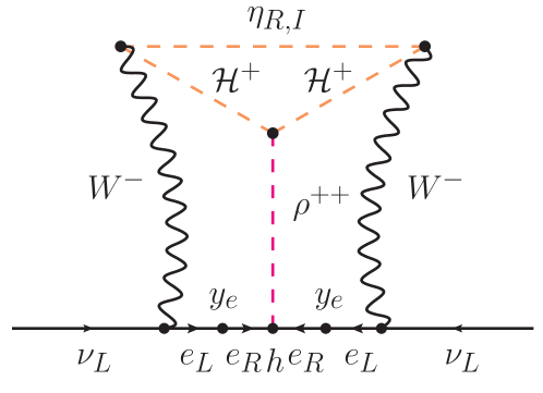
Figure 1: 3-loop neutrino masses in the cocktail model. The inert doublet $\eta$ is split into its real and imaginary parts, $\eta^{0}=\frac{1}{\sqrt{2}}(\eta_{R}+i\,\eta_{I})$, due to the scalar potential terms proportional to $\lambda_{5}$. $\mathcal{H}^{+}\equiv\mathcal{H}^{+}_{1,2}$ represent the singly charged scalars in the model, obtained after diagonalizing the mass matrix of the $\left\{S^{+},\eta^{+}\right\}$ states.

The 3-loop diagram leading to neutrino masses in the cocktail model is shown in Fig. 1. In the unitary gauge this diagram is the only diagram contributing to the neutrino mass matrix. However, in order to understand how to maximize the contribution of this diagram to the neutrino mass matrix, it is more useful to calculate all diagrams in Feynman-’t Hooft gauge. This is discussed in detail in Appendix A.1.

In an analogous way to the well-known scotogenic model [40], the diagram shown in Fig. 1 vanishes in the limit $m_{\eta_{R}}^{2}-m_{\eta_{I}}^{2}\propto\lambda_{5}\to 0$, since in this limit the model conserves lepton number. We can then write the neutrino mass matrix in the cocktail model as:

$$\left(\mathcal{M}_{\nu}\right)_{ij}=\frac{\lambda_{5}}{(16\pi^{2})^{3}}\frac{m_{i}\,h_{ij}\,m_{j}}{m_{\rho^{++}}}\,F_{\rm Cocktail}\,,$$ (19)

where $m_{i}$ and $m_{j}$ are charged lepton masses. Here we have hidden all the complexities of the calculation in the dimensionless factor $F_{\rm Cocktail}$. This factor contains the loop integrals, depending on the masses of the scalars, and prefactors containing coupling constants, etc, see Appendix A.1.

3.2 Results

The cocktail model is an example of a type-II-seesaw-like model. In this class of models, the neutrino mass matrix is proportional to a symmetric Yukawa matrix,

$$\mathcal{M}_{\nu}\sim Y\,\frac{v^{2}}{\Lambda}\,,$$ (20)

with $Y_{ij}=Y_{ji}$ and $\Lambda$ some generic mass scale. This allows one to fit the observed neutrino masses and mixing angles in a trivial way. Furthermore, the tight relation given in Eq. (20) implies very specific predictions for ratios of CLFV observables and strongly reduces the number of free parameters in the model. As we will discuss now, this has very important consequences.

From the experimental data we can reconstruct the neutrino mass matrix in the flavor basis as

$${\cal M}_{\nu}=U^{\ast}\,\widehat{\cal M}_{\nu}\,U^{\dagger}\,.$$ (21)

This allows us to calculate the Yukawa $h$ necessary to fit the experimental data using the expression in Eq. (19). We find

$$h=(16\pi^{2})^{3}\,\frac{m_{\rho^{++}}}{\lambda_{5}\,F_{\rm Cocktail}}\,{\widehat{\cal M}_{e}}^{-1}\,{\cal M}_{\nu}\,{\widehat{\cal M}_{e}}^{-1}\,.$$ (22)

where $\widehat{\cal M}_{e}$ is the diagonal matrix with the measured charged lepton masses, see Eq. (12).

Let us first make a rough numerical estimate. Choosing normal hierarchy ($m_{\nu_{1}}\to 0$) and $\delta=0$ for simplicity and inserting $m_{\rho^{++}}=800$ GeV, which is roughly the current experimental bound from LHC data [41, 42, 43], we find

$$h\simeq\begin{pmatrix}46000&450&5.7\\ 450&8.1&0.36\\ 5.7&0.36&0.026\end{pmatrix}\Big{(}\frac{m_{\rho^{++}}}{\rm 800\hskip 2.84526ptGeV}\Big{)}\Big{(}\frac{1}{\lambda_{5}}\Big{)}\Big{(}\frac{1}{F_{\rm Cocktail}}\Big{)}.$$ (23)

These values are obviously much too large to be realistic. We therefore searched the parameter space, intending to identify regions, in which $h$ can fulfill the bounds from perturbativity and lepton flavor violation searches. This search was done in two steps.

First, we maximize $F_{\rm Cocktail}$ and $\lambda_{5}$. For $\lambda_{5}$ we use $\lambda_{5}=4\pi$, the largest value allowed by perturbativity. We then scanned all free mass parameters entering in $F_{\rm Cocktail}$, for details see appendix A.1. Generally speaking, $F_{\rm Cocktail}$ is maximized when $\mu_{1}$, $\mu_{2}$ and $\kappa$ take the largest values allowed, while the remaining free mass eigenvalues of the model take the lowest possible values allowed by experimental searches. The maximal value of $F_{\rm Cocktail}$ found in this numerical scan is $F_{\rm Cocktail}^{\rm max}\simeq 192$. We will use this number in all plots below. This choice is conservative in the sense that the Yukawa couplings $h_{ij}$ will be larger for all other choices, thus constraints from charged lepton flavor violation searches will only be more stringent in other parts of the parameter space.

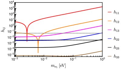
Figure 2: Yukawa couplings $h_{ij}$ as function of the lightest neutrino mass, calculated with $F_{\rm Cocktail}^{\rm max}$. These Yukawas should therefore be understood as lower limits. In both plots we have used the best fit point data from the global oscillation fit [38], except $\delta=0$. The plot to the left shows the case $(\alpha_{12},\alpha_{13})=(0,0)$, the plot on the right $(\alpha_{12},\alpha_{13})=(\pi,0)$. The dashed gray (black) lines in the background are rough estimates for the typical size that the Yukawa couplings should have, in order to satisfy limits from muon (tau) CLFV decays. These lines are only for orientation.

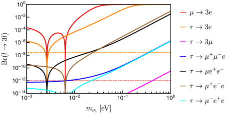
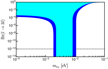
Figure 3: Br($l_{i}\to l_{j}l_{k}l_{m}$) as function of the lightest neutrino mass. To the left, all different combinations of lepton generations are considered using the b.f.p. of oscillation data and $\alpha_{12}=\pi$ and $2\delta-\alpha_{13}=0$. To the right, Br($\mu\to 3\,e$) scanned over the uncertainty in neutrino oscillation data is shown. The light and dark blue areas correspond to the $1\,\sigma$ and $3\,\sigma$ uncertainties, respectively. This plot scans over the Majorana phases.

Once $F_{\rm Cocktail}^{\rm max}$ is fixed, one can scan over the free parameters in the neutrino sector. Oscillation data [38] fixes rather well $\Delta m^{2}_{\rm Atm}$, $\Delta m^{2}_{\odot}$ and all three mixing angles; there is also an indication for a non-zero value of $\delta$. This leaves us with three essentially free parameters, the two Majorana phases and $m_{\nu_{1}}$, equivalent to the overall neutrino mass scale, for which there are only upper limits from neutrinoless double beta ($0\nu\beta\beta$) decay [44, 45] and cosmology [46]. We note that there is a slight preference in the data for normal hierarchy (NH, also called normal ordering) over inverted hierarchy (IH).

In Fig. 2 we plot the absolute values of the 6 independent entries in the Yukawa matrix $h$ as a function of $m_{\nu_{1}}$. The oscillation data have been fixed at their best fit point (b.f.p.) values, except $\delta=0$ for simplicity. The plot on the left was obtained with vanishing Majorana phases, whereas the one on the right takes $(\alpha_{12},\alpha_{13})=(\pi,0)$. Given that we used $F_{\rm Cocktail}^{\rm max}$ in this plot, the numerical values of $h_{ij}$ are much smaller than in Eq. (23), but $h_{11}$ is still in the non-perturbative region everywhere in the left plot. In the right plot, however, there are two special points, where cancellations among different contributions of the neutrino mass eigenstates lead to a vanishing value for either $h_{11}$ or $h_{12}$. Such cancellations are well known in studies of $0\nu\beta\beta$ decay. The effective Majorana mass, $m_{ee}$, depends on the Majorana phases in the same way as $h_{11}$. As in $m_{ee}$, one can therefore not obtain a cancellation for the cases (i) NH without Majorana phases, and (ii) IH for any choice of parameters. The cocktail model can therefore explain neutrino data only for normal hierarchy and some particular combination of Majorana phases, as we are going to discuss now in some more detail.

As Fig. 2 demonstrates, only in some exceptional points can $h_{11}$ be small enough to enter the perturbative region. We therefore scanned over $(\alpha_{12},\alpha_{13})$ and $m_{\nu_{1}}$, in the full $3\,\sigma$ range of oscillation data. In this scan, we calculate the CLFV observable Br($l_{i}\to l_{j}l_{k}l_{m}$), with different combinations of lepton flavors, for the minimal value of $m_{\rho^{++}}$ allowed by LHC data. Fig. 3 to the left shows Br($l_{i}\to l_{j}l_{k}l_{m}$) for all different combinations of $i,j,k,m$ using the b.f.p. of neutrino oscillation data. The most stringent constraint on the model comes from the experimental upper limit on Br($\mu\to 3\,e$)$\leq 10^{-12}$ [47]. The plot to the right then shows the allowed regions in parameter space, scanning over the complete range of oscillation parameters and phases. All acceptable points lie in the range $m_{\nu_{1}}=(2-10)$ meV.

Fig. 4 shows a scan over the allowed range of Majorana phases and the lightest neutrino mass. The plot to the left shows the plane ($\alpha_{13},\alpha_{12}$), the one to the right ($\alpha_{12},m_{\nu_{1}}$). The model can fulfill the constraint from Br($\mu\to 3\,e$) only in a very narrow range of phases. In particular, $\alpha_{12}$ has to be close to $\pi$ in all points, while also $m_{\nu_{1}}$ is fixed in a rather narrow interval.

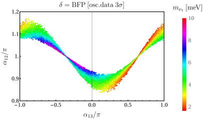
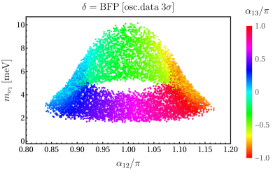
Figure 4: Allowed parameter space for $\alpha_{12}$, $\alpha_{13}$ and $m_{\nu_{1}}$. Note that $m_{\nu_{1}}$ is shown in units of meV. Neutrino oscillation data was scanned over the $3\,\sigma$ uncertainties, except $\delta$ which is taken at its best fit value for simplicity.

Finally we note that the acceptable points of the model lie in regions of parameter space where the $0\nu\beta\beta$ decay observable $m_{ee}$ is unmeasurably small. There is, however, a 1-loop short-range diagram contributing to $0\nu\beta\beta$ decay in the cocktail model [48], see Fig. 5. This diagram depends on the same parameters as the 3-loop neutrino mass diagram in Fig. 1. In particular, note that the sum over $\eta_{R,I}$ generates the same dependence on $\lambda_{5}$ as for the neutrino mass.

We have calculated this diagram and estimated its contribution to the $0\nu\beta\beta$ decay half-life, including the QCD running of the short-range operator [49, 50]. Using the same mass parameters that maximize the 3-loop diagram, in particular $m_{\rho^{++}}=800$ GeV, the current limit on the half-life of ¹³⁶Xe [44] imposes a limit on $h_{11}$ of roughly $|h_{11}|\raise 1.29167pt\hbox{$\;<$\kern-7.5pt\raise-4.73611pt\hbox{$\sim\;$}}5\times 10^{-4}$. This limit is around a factor $\sim 7$ more stringent than the one obtained from the upper limit on Br($\mu\to 3\,e$). 

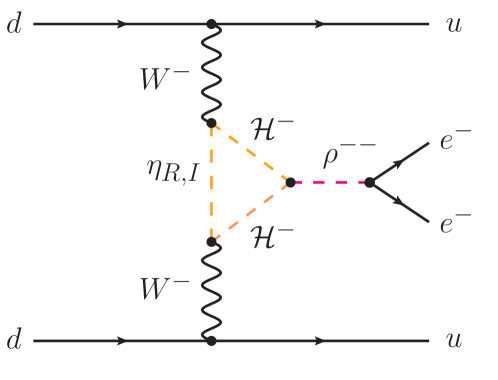
Figure 5: 1-loop neutrinoless double beta decay diagram in the cocktail model.

We can conclude that the cocktail model is severely constrained from perturbativity arguments and from searches for CLVF. The model has acceptable points only within a narrow window of $m_{\nu_{1}}$ and for particular combinations of the Majorana phases.

4 KNT model

We continue with the KNT model [11]. This was the first radiative neutrino mass model at 3-loop order proposed.

4.1 The model

In addition to the SM particles, the KNT model contains three copies of the fermionic singlet $N$ and two singly-charged singlet scalars $X$ and $S$. A discrete $\mathbb{Z}_{2}$ symmetry is imposed, under which $S$ and $N$ are odd and the rest of particles in the model are even. The quantum numbers of the new particles in the KNT model are given in Table 6.

	generations	$\mathrm{SU(3)}_{c}$	$\mathrm{SU(2)}_{L}$	$\mathrm{U(1)}_{Y}$	$\mathbb{Z}_{2}$
$X$	1	${\bf 1}$	${\bf 1}$	$1$	$+$
$S$	1	${\bf 1}$	${\bf 1}$	$1$	$-$
$N$	3	${\bf 1}$	${\bf 1}$	$0$	$-$

Table 6: New particles in the KNT model with respect to the SM.

The Lagrangian of the model contains the following pieces

$$-\mathcal{L} \supset f\,\overline{L^{c}}\,L\,X+g^{\ast}\,\overline{N^{c}}\,e_{R}\,S+\frac{1}{2}M_{N}\overline{N^{c}}N+\mathrm{h.c.}\,,$$ (24)

where we have omitted $\mathrm{SU(2)_{L}}$ and flavor indices to simplify the notation. We note that $f$ is an antisymmetric $3\times 3$ Yukawa matrix, while $M_{N}$ is a symmetric $3\times 3$ Majorana mass matrix, which we take to be diagonal without loss of generality. The scalar potential of the model also contains additional terms besides those in the SM. These are given by

$$\mathcal{V} \supset M_{X}^{2}|X|^{2}+M_{S}^{2}|S|^{2}+\frac{1}{2}\lambda_{1}\,|X|^{4}+\frac{1}{2}\lambda_{2}\,|S|^{4}+\lambda_{12}\,|X|^{2}|S|^{2}$$

$$+\lambda_{H}^{(1)}\,|H|^{2}|X|^{2}+\lambda_{H}^{(2)}\,|H|^{2}|S|^{2}+\frac{1}{4}\,\left[\lambda_{S}\,(XS^{\ast})^{2}+\mathrm{h.c.}\right]\,.$$ (25)

The presence of the $\lambda_{S}$ quartic coupling precludes the definition of a conserved lepton number. Indeed, one can easily see that the simultaneous presence of the Lagrangian terms in Eqs. (24) and (4.1) breaks lepton number in two units. The masses of the physical scalar states in the KNT model are given by

$$m_{H}^{2} = \lambda\,v^{2}\,,$$ (26)

$$m_{s_{1}}^{2} = M_{X}^{2}+\frac{1}{2}\,\lambda_{H}^{(1)}\,v^{2}\,,$$ (27)

$$m_{s_{2}}^{2} = M_{S}^{2}+\frac{1}{2}\,\lambda_{H}^{(2)}\,v^{2}\,.$$ (28)

We also note that the lightest $\mathbb{Z}_{2}$-odd state in the KNT model is completely stable. Assuming the hierarchy $M_{N_{1}}<m_{s_{1}}<m_{s_{2}}$, this state is the lightest fermion singlet, which then constitutes a good DM candidate. In fact, the KNT model is historically the first radiative neutrino mass theory with a stable DM candidate running in the loop.

Neutrino masses

Figure 6: 3-loop neutrino masses in the KNT model.

The $\mathbb{Z}_{2}$ symmetry forbids the standard Higgs Yukawa coupling with the lepton doublet $L$ and the $N$ singlets. Therefore, the usual type-I seesaw contribution at tree-level is absent. Instead, neutrino masses are generated at 3-loop order as shown in Fig. 6. The neutrino mass matrix is given by

$$\left(\mathcal{M}_{\nu}\right)_{ij}=\frac{2\lambda_{S}}{(16\pi^{2})^{3}}\sum_{\alpha\beta a}\frac{m_{\alpha}m_{\beta}}{M_{N_{a}}}f_{i\alpha}f_{j\beta}g_{\alpha a}g_{\beta a}\,F_{\rm KNT}\,,$$ (29)

where $m_{\alpha}$ is the mass of the $\ell_{\alpha}$ charged lepton and $F_{\rm KNT}$ is a loop function that depends on the masses of the scalars and fermions running in the loops. More information about this function can be found in Appendix A.2.

It is important to stress that in the KNT model, each entry in $(\mathcal{M}_{\nu})_{ij}$ contains the sum over the SM charged lepton masses. Therefore, different from the other models discussed in this paper, the suppression of the entries in $\mathcal{M}_{\nu}$ is at most $m_{\mu}^{2}$. The neutrino fit can then reproduce experimental data with Yukawas which are considerably smaller than in the cocktail or AKS models.

4.2 Results

We start this section again with a discussion of the neutrino mass fit. The coupling $f$ in Eq. (24) is antisymmetric, thus the determinant of the neutrino mass matrix in Eq. (29) is zero, implying that one neutrino is massless. This is reminiscent of the 2-loop Babu-Zee model of neutrino mass [3, 4], where the same singly charged scalar is used. In our fitting procedure we use therefore an adapted version of the solution found in [51, 52] for the Babu-Zee model.

The procedure consists of two steps. First, because det$(f)=0$, the matrix has one eigenvector ${\bf a}=(f_{23},-f_{13},f_{12})$, which is also an eigenvector of $\mathcal{M}_{\nu}$:

$$\widehat{\cal M}_{\nu}\,U^{T}{\bf a}=0\,.$$ (30)

This implies three equations, one of which is trivial, while the other two allow to express the ratios $(f_{13}/f_{12},f_{23}/f_{12})$ as functions of the neutrino angles and phases only. These solutions depend on the neutrino mass hierarchy.

Next, we can write the neutrino mass matrix as

$$\mathcal{M}_{\nu}=-c\,f\,M_{\rm aux}\,f\,.$$ (31)

$c$ contains all global constants, we have used $f^{T}=-f$ and $M_{\rm aux}$ is an auxiliary matrix, which is complex symmetric. This defines a set of 6 complex equations relating the entries in $M_{\rm aux}$ to neutrino data. With three independent entries $f_{ij}$, we can use three of the six equations to express three entries in $M_{\rm aux}$ as a function of the remaining ones, neutrino data and $f_{ij}$. The resulting equations are very lengthy and not at all illuminating, so we do not present them here.

The definition of $M_{\rm aux}$ in Eq. (31) shows that

$$M_{\rm aux}={\widehat{\cal M}_{e}}\,g\left({\widehat{M}^{\rm eff}}\right)^{-1}g^{T}{\widehat{\cal M}_{e}}$$ (32)

where

$$\left({\widehat{M}^{\rm eff}}\right)^{-1}=\begin{pmatrix}\frac{F_{KNT}(r^{X}_{1},r^{S}_{1})}{M_{N_{1}}}&0&0\\ 0&\frac{F_{KNT}(r^{X}_{2},r^{S}_{2})}{M_{N_{2}}}&0\\ 0&0&\frac{F_{KNT}(r^{X}_{3},r^{S}_{3})}{M_{N_{3}}}\end{pmatrix}\,,$$ (33)

and $r^{X}_{i}=(m_{s_{1}}/M_{N_{i}})^{2}$, $r^{S}_{i}=(m_{s_{2}}/M_{N_{i}})^{2}$. With $M_{\rm aux}$ being complex symmetric, we can use a suitably modified [53, 54] Casas-Ibarra parametrization [55] to express the matrix $g$ as

$$g=\sqrt{{\widehat{M}^{\rm eff}}}{\cal R}\,\sqrt{\hat{M}_{\rm aux}}\,U_{\rm aux}^{T}\left({\widehat{\cal M}_{e}}\right)^{-1}.$$ (34)

${\hat{M}_{\rm aux}}$ and $U_{\rm aux}$ are the eigenvalues and eigenvectors of the auxiliary matrix $M_{\rm aux}$. Although in principle it would be possible to determine ${\hat{M}_{\rm aux}}$ and $U_{\rm aux}$ in terms of the input neutrino data analytically, in practice we find these two matrices numerically for any input point of experimental data and choice of free parameters. Finally, ${\cal R}$ is a $3\times 3$ orthogonal matrix.

In summary, neutrino oscillation data provides 6 constraints: $\Delta m_{\rm Atm}^{2}$, $\Delta m_{\odot}^{2}$, three angles and the CP-phase $\delta$. A number of free parameters can then be scanned over, using the above procedure. In the neutrino sector we still have $\alpha_{12}$. The matrix $f$ is fixed from experimental data, up to the overall scale of the matrix. We choose $f_{12}$ as the free parameter. The matrix ${\cal R}$, in the most general case, contains 3 complex angles. There are 3 right-handed neutrino masses, $M_{N_{i}}$, and 2 scalar masses, $m_{s_{1,2}}$. And, finally, we can use 3 of the 6 equations for $M_{\rm aux}$ to eliminate some particularly chosen $(M_{\rm aux})_{ij}$. This leaves as free inputs the remaining 3 entries in $M_{\rm aux}$.

Up to now, we have been completely general in our discussion. However, there is still a certain freedom as to which 3 entries in $(M_{\rm aux})_{ij}$ we fix via 3 of the equations defined by Eq. (31). In practice, we choose to solve for $(M_{\rm aux})_{22}$, $(M_{\rm aux})_{23}$ and $(M_{\rm aux})_{33}$ and assume $(M_{\rm aux})_{1k}=0$. This particular choice is motivated by the observation that in this limit all terms in $g\propto 1/m_{e}$ disappear. In other words, this solution guarantees that the contribution to $\mu\to e\gamma$ and $\tau\to e\gamma$ from loops involving $s_{2}$ and $N_{i}$ are automatically absent in our scans, due to $g_{1k}=0$ $\forall k$. Our ansatz is therefore the optimal choice for minimizing fine-tuning on the other parameters in $g$. 

Before we explore the remaining parameter space of the model, we must consider lower limits on the masses of the charged scalars from accelerator searches. LEP provides a lower limit on charged particles decaying to leptons plus missing momentum, which will essentially rule out all values of $m_{s_{1}}$ below 100 GeV [39] and similarly for $m_{s_{2}}$, unless $M_{N_{1}}$ is close to $m_{s_{2}}$.  At the LHC there is currently no specific search for particles with the quantum numbers of $S$ and $X$. However, slepton pair production with their subsequent decays to a lepton plus a neutralino provide the same signal and thus, we can make a reinterpretation of the corresponding searches at CMS [56] and ATLAS [57]. The CMS slepton search [56] is based on $35.9/$fb, while ATLAS’ chargino and slepton search [57] uses $139/$fb. The ATLAS limits are correspondingly more stringent and we will therefore discuss these. We have implemented the KNT model in SARAH [58, 59] and generated SPheno routines [60, 61] and model files for MadGraph [62, 63, 64]. We have then calculated cross sections with MadGraph to recast the results of [57]. For $s_{1}$ the mass range between (very roughly) $m_{s_{1}}=(250-400)$ GeV is excluded by this search. The range $m_{s_{1}}=(100-250)$ is currently unconstrained, due to large backgrounds in [57]. For $s_{2}$ the limits are even weaker, unless $m_{s_{2}}-M_{N_{1}}$ is larger than ($50-70$) GeV, depending on $m_{s_{2}}$.

Let us now turn to the discussion of CLFV. Consider first the antisymmetric Yukawa coupling $f$. Neutrino data requires all three elements of $f$ to be non-zero, thus there will always be a non-zero value for the three possible decays $\mu\to e\gamma$, $\tau\to e\gamma$ and $\tau\to\mu\gamma$. The constraint from $\mu\to e\gamma$ is the most stringent one. However, since we still have the overall scale of $f$ as a free parameter, in our choice the value of $f_{12}$, we can use it to fix Br($\mu\to e\gamma$) to the upper limit (present or future) for any point in the parameter space. Since the neutrino mass matrix is proportional to the square of the matrices $f$ and $g$ however, once this choice is made there is no longer any overall scaling freedom in the coupling $g$. Putting the calculated Br($\mu\to e\gamma$) to equal the experimental bound will generate the smallest values for the entries of $g$ allowed in the model parameter space. A smaller upper limit on Br($\mu\to e\gamma$) will lead to larger $g$ and thus more stringent constraints from $\tau\to\mu\gamma$.

We then scanned over the remaining parameters of the model numerically. Consider first the case of NH. Some examples for Br($\tau\to\mu\gamma$) are shown in Fig. 7. In this plot we have chosen the fixed value $m_{s_{1,2}}=100$ GeV, corresponding to the experimental lower limit, and the three right-handed neutrino masses all equal to a common $M_{N}$.  The points are scanned over the allowed $3\,\sigma$ ranges for the neutrino data for NH. The size of the largest entry in $g$ is color-coded in the points. The plot to the left has been calculated for the current experimental limit on Br($\mu\to e\gamma$)$<4.2\times 10^{-13}$ [65], the plot to the right is for the expected future limit Br($\mu\to e\gamma$)$<6\times 10^{-14}$ [66]. For the choice of $m_{s_{1,2}}=100$ GeV no valid point with $g_{ij}\leq 4\pi$ $\forall ij$ remains in the parameter space. Constraints are more stringent for IH, and therefore the same conclusion is reached.

Figure 7: Calculated values for Br($\tau\to\mu\gamma$) as function of the common fermion mass $M_{N}$, for the current lower limit on $m_{s_{1}}=m_{s_{2}}=100$ GeV. To the left, with current experimental limits; to the right for the expected future experimental limits. The required size of the Yukawas is color-coded. Bluish-grey points mean that at least one entry in $g$ is larger than $4\pi$.

Figure 8: Calculated values for Br($\tau\to\mu\gamma$) as function of the scalar mass $m_{s}$ for different values of $M_{N}$ (color coded). Bluish points are ruled out by non-perturbative couplings. To the left, with current experimental limits; to the right for the expected future experimental limit on Br($\mu\to e\gamma$).

We therefore scanned over $m_{s_{1,2}}\equiv m_{S}$ and $M_{N_{i}}$ simultaneously. The results are shown in Fig. 8. Here, $M_{N_{i}}$ are varied within $20\%$ of a common $M_{N}$. The range of $M_{N}$ is color-coded in the points. Again, the plot to the left is for the current bound on Br($\mu\to e\gamma$), while the plot to the right is for the future bound. In these plots, points with non-perturbative couplings are shown in bluish color. This bound eliminates all points below roughly $M_{N}={\cal O}(100)$ GeV already with the current experimental bound on Br($\mu\to e\gamma$), see however the discussion below. We show only the cases with a trivial ${\cal R}$ matrix. For non-zero angles in ${\cal R}$ the results look similar, although fewer points lie in the perturbative regime.

The combined constraints of perturbativity and future limits from CLFV searches would put a lower bound on $m_{S}$ roughly of order ($180-200$) GeV. This limit becomes stronger for lower values of $M_{N}$, as the plots shows.

The above discussion is strictly valid only for the case where the three right-handed neutrinos have similar masses. For hierarchical right-handed neutrinos the constraints are usually dominated by the lightest of these. There exist, however, exceptional points in the parameter space, where the contributions to Br($\mu\to e\gamma$) from the three different neutrinos conspire to (nearly) cancel each other. This is shown in Fig. 9. The figure shows Br($\tau\to\mu\gamma$) as a function of the “lightest” right-handed neutrino mass, for different choices of $M_{N_{2,3}}$. Br($\tau\to\mu\gamma$) is dominated by the lightest mass eigenstate, except in some particular points, where cancellations occur. Figs. 7 and 8 do not cover these exceptional combinations of parameters.

Figure 9: Calculated values for Br($\tau\to\mu\gamma$) as function of the lightest right-handed neutrino mass $M_{N_{1}}$ for different choices of $M_{N_{2,3}}$ and two different scalar masses $m_{S}$ (left and right). The calculation uses for simplicity the b.f.p. for neutrino data.

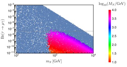
Figure 10: Same as Fig. 8 but for IH for the neutrino masses. Bluish points are excluded due to perturbativity arguments.

We have repeated the scans discussed above also for the case of IH. An example is shown in Fig. 10. IH requires larger Yukawa couplings, since now two neutrino have masses of order $\sqrt{\Delta m^{2}_{\rm Atm}}$. Thus, many more points in the parameter space are ruled out due to the perturbativity constraint. This pushes both, fermion as well as the scalar, masses to larger values. Indeed, already with current constraints there are no points with $m_{S}$ below roughly 600 GeV.

Finally, let us mention that in the KNT model there is no short-range diagram contributing to $0\nu\beta\beta$ decay. Given that the KNT model predicts one (nearly) massless neutrino, it predicts both, an upper and a lower limit for $0\nu\beta\beta$ decay. For normal [inverted] hierarchy the allowed range is roughly $m_{ee}\sim(1-5)$ meV [$(20-50)$ meV]. Observing $0\nu\beta\beta$ decay outside this range would rule out the KNT model as an explanation for the experimental neutrino oscillation data.

5 AKS model

A general class of models is represented by the AKS model [12]. In this case the particle content is extended to include new scalars and fermions.

5.1 The model

The AKS model extends the usual 2HDM with the real scalar singlet $\varphi$, the singly charged scalar $S$ and three generations of singlet fermions $N$. Even though a more minimal version with only two generations of $N$ is possible, we will consider three in the following. The fields $S$, $\varphi$ and $N$ are assumed to be odd under the $\mathbb{Z}_{2}$ parity, while the rest of the particles are even. The quantum numbers of the new particles in the AKS model are given in Table 7.

	generations	$\mathrm{SU(3)}_{c}$	$\mathrm{SU(2)}_{L}$	$\mathrm{U(1)}_{Y}$	$\mathbb{Z}_{2}$
$\varphi$	1	${\bf 1}$	${\bf 1}$	$0$	$-$
$S$	1	${\bf 1}$	${\bf 1}$	$1$	$-$
$N$	3	${\bf 1}$	${\bf 1}$	$0$	$-$

Table 7: New particles in the AKS model with respect to the 2HDM.

As explained in Sec. 2, an additional softly-broken $\mathbb{Z}_{2}$ symmetry is introduced to avoid dangerous flavor changing neutral currents. We choose to follow [12] and use this symmetry to couple one of the scalar doublets ($\Phi_{1}$) only to leptons, and the other ($\Phi_{2}$) only to quarks. Due to this choice, the Yukawa couplings of the model are given in Eq. (5), along with the Yukawa

$$-\mathcal{L}\supset Y^{\ast}\,\overline{N^{c}}\,e_{R}\,S+\mathrm{h.c.}\,.$$ (35)

One can also write Majorana masses for the $N$ singlets,

$$-\mathcal{L}_{N}=\frac{1}{2}M_{N}\overline{N^{c}}N+\mathrm{h.c.}\,,$$ (36)

with $M_{N}$ a symmetric matrix. The scalar potential of the model is given by

$$\mathcal{V} \supset m_{1}^{2}|\Phi_{1}|^{2}+m_{2}^{2}|\Phi_{2}|^{2}+\left(\mu_{12}^{2}\,\Phi_{1}^{\dagger}\Phi_{2}+\mathrm{h.c.}\right)+\frac{1}{2}\lambda_{1}\,|\Phi_{1}|^{4}+\frac{1}{2}\lambda_{2}\,|\Phi_{2}|^{4}$$

$$+\lambda_{3}\,|\Phi_{1}|^{2}|\Phi_{2}|^{2}+\lambda_{4}\,|\Phi_{1}^{\dagger}\Phi_{2}|^{2}+\frac{1}{2}\left[\lambda_{5}\,(\Phi_{1}^{\dagger}\Phi_{2})^{2}+\mathrm{h.c.}\right]$$

$$+\lambda_{\Phi S}^{(1)}\,|\Phi_{1}|^{2}|S|^{2}+\lambda_{\Phi S}^{(2)}\,|\Phi_{2}|^{2}|S|^{2}+\frac{1}{2}\lambda_{\Phi\varphi}^{(1)}\,|\Phi_{1}|^{2}\varphi^{2}+\frac{1}{2}\lambda_{\Phi\varphi}^{(2)}\,|\Phi_{2}|^{2}\varphi^{2}+\left[\kappa\,\Phi_{1}\,\Phi_{2}\,S^{\ast}\,\varphi+\mathrm{h.c.}\right]$$

$$+\frac{M_{\varphi}^{2}}{2}\varphi^{2}+M_{S}^{2}|S|^{2}+\frac{1}{2}\lambda_{S}\,|S|^{4}+\frac{1}{4!}\lambda_{\varphi}\varphi^{4}+\frac{1}{2}\xi\,\varphi^{2}|S|^{2}\,.$$ (37)

As usual, we have omitted $\mathrm{SU(2)}_{L}$ indices in the previous expression. We point out that lepton number would be restored in the limit $\kappa\to 0$. The presence of this coupling breaks lepton number in one unit.

After electroweak symmetry breaking, the doublet scalars $\Phi_{1}$ and $\Phi_{2}$ get mixed. The mass eigenstates resulting from this mixing are the SM Higgs, another Higgs, a new charged scalar, and a pseudoscalar. The charged and neutral Goldstone bosons are absorbed by the $Z$ and $W$ gauge bosons. The mass matrix for the CP-even neutral states in the basis $\mathcal{H}^{0}=\text{Re}\,(\Phi_{1}^{0},\Phi_{2}^{0})^{T}$ is given by

$$\mathcal{M}^{2}_{\mathcal{H}^{0}}=\left(\begin{array}[]{cc}\lambda_{1}v_{1}^{2}-\mu_{12}^{2}\,\tan\beta&v_{1}v_{2}\left(\lambda_{3}+\lambda_{4}+\lambda_{5}\right)+\mu_{12}^{2}\\ v_{1}v_{2}\left(\lambda_{3}+\lambda_{4}+\lambda_{5}\right)+\mu_{12}^{2}&\lambda_{2}v_{2}^{2}-\mu_{12}^{2}\,\cot\beta\end{array}\right)\,.$$ (38)

The CP-odd neutral scalar mass matrix in the basis $\mathcal{A}^{0}=\text{Im}\,(\Phi_{1}^{0},\Phi_{2}^{0})^{T}$ is

$$\mathcal{M}^{2}_{\mathcal{A}^{0}}=\left(\begin{array}[]{cc}-v_{2}^{2}\lambda_{5}-\mu_{12}^{2}\,\tan\beta&v_{1}v_{2}\lambda_{5}+\mu_{12}^{2}\\ v_{1}v_{2}\lambda_{5}+\mu_{12}^{2}&-v_{1}^{2}\lambda_{5}-\mu_{12}^{2}\,\cot\beta\end{array}\right)\,.$$ (39)

One finds a massless state, the Goldstone boson that becomes the longitudinal component of the $Z$ boson. The other state has a mass

$$m^{2}_{\mathcal{A}^{0}}=-\left(v_{1}v_{2}\lambda_{5}+\mu_{12}^{2}\right)\,\frac{v^{2}}{v_{1}v_{2}}\,,$$ (40)

while the mass of the $Z$ boson is $m_{Z}^{2}=\frac{1}{4}v^{2}(g_{1}^{2}+g_{2}^{2})$. The mass matrix for the charged states in the $\mathcal{H}^{\pm}=(\Phi_{1}^{\pm},\Phi_{2}^{\pm})^{T}$ basis is

$$\mathcal{M}^{2}_{\mathcal{H}^{\pm}}=\left(\begin{array}[]{cc}-\frac{1}{2}v_{2}^{2}\,\left(\lambda_{4}+\lambda_{5}\right)-\mu_{12}^{2}\,\tan\beta&\frac{1}{2}v_{1}v_{2}\,\left(\lambda_{4}+\lambda_{5}\right)+\mu_{12}^{2}\\ \frac{1}{2}v_{1}v_{2}\,\left(\lambda_{4}+\lambda_{5}\right)+\mu_{12}^{2}&-\frac{1}{2}v_{1}^{2}\,\left(\lambda_{4}+\lambda_{5}\right)-\mu_{12}^{2}\,\cot\beta\end{array}\right)\,.$$ (41)

Again, after diagonalization one obtains a massless state, identified with the Goldstone boson that becomes the longitudinal part of the $W$ boson, and a massive physical charged scalar with mass

$$m^{2}_{\mathcal{H}^{\pm}}=-\left(\frac{\mu_{12}^{2}}{v_{1}v_{2}}+\frac{\lambda_{4}+\lambda_{5}}{2}\right)v^{2}\,.$$ (42)

The mass of the $W$ boson is given by the standard expression $m_{W^{\pm}}^{2}=\frac{1}{4}g_{2}^{2}v^{2}$. Finally, the masses of the singlet scalars $\varphi$ and $S$ are

$$m_{\varphi}^{2} =M_{\varphi}^{2}+\frac{1}{2}\left(\lambda_{\Phi\varphi}^{(1)}\,v_{1}^{2}+\lambda_{\Phi\varphi}^{(2)}\,v_{2}^{2}\right)\,,$$ (43)

$$m_{S^{+}}^{2} =M_{S}^{2}+\frac{1}{2}\left(\lambda_{\Phi S}^{(1)}\,v_{1}^{2}+\lambda_{\Phi S}^{(2)}\,v_{2}^{2}\right)\,.$$ (44)

As in the cocktail model, the lightest $\mathbb{Z}_{2}$-odd state in the AKS model is stable and can constitute a DM candidate.

Neutrino masses

Figure 11: 3-loop neutrino masses in the AKS model. $\mathcal{H}^{-}\equiv\mathcal{H}^{-}_{1,2}$ represent the singly charged scalars in the model, obtained after diagonalizing the mass matrix of the $\left\{\Phi_{1}^{-},\Phi_{2}^{-}\right\}$ states.

In the AKS model, neutrino masses are induced at 3-loop order, as shown in the diagrams of Fig. 11. The resulting neutrino mass matrix is given by

$$\left(\mathcal{M}_{\nu}\right)_{ij}=\frac{\kappa^{2}\,\tan^{2}\beta}{(16\pi^{2})^{3}}\,\sum_{\alpha\beta}\frac{m_{i}\,Y_{i\alpha}Y_{j\beta}\,m_{j}}{(M_{N})_{\alpha\beta}}\,F_{\rm AKS}\,,$$ (45)

where $m_{i}$ is the mass of the $i$-th charged lepton and $F_{\rm AKS}$ is a dimensionless loop function that depends on the masses of the scalars and fermions in the loop. More details about the calculation of this loop function can be found in Appendix A.3.

The Yukawa matrix $Y$ in the AKS model does not have any specific symmetry. Therefore, this model represents the general class of models in which the Yukawa matrices can be described by using a generalization of the Casas-Ibarra parametrization [55] (see also [53, 54]).

5.2 Results

The Yukawa structure of the neutrino mass matrix shown in Eq. (45) resembles that of the type-I seesaw. In order to fit the experimental oscillation data, we use the Casas-Ibarra parametrization introducing the neutrino mass matrix in the flavor basis given in Eq. (21). We find that

$$Y=\frac{i\,(16\pi^{2})^{3/2}}{\kappa\,\tan\beta}\,{\cal R}\,\sqrt{M_{N}/F_{\rm AKS}}\,\sqrt{\widehat{\cal M}_{\nu}}\,U^{\dagger}\,\widehat{\cal M}^{-1}_{e}\,,$$ (46)

where $M_{N}$ has been taken to be diagonal and ${\cal R}$ is an arbitrary complex $3\times 3$ orthogonal matrix. We include $F_{\rm AKS}$ as it is, in general, a function of the eigenvalues of $M_{N}$, see Appendix A.3. Similar to the KNT model, the presence of $\widehat{\cal M}^{-1}_{e}$ in the fit, implies the enhancement of each column of the Yukawa matrix in terms of the charged lepton masses, i.e. $Y_{\alpha i}\propto 1/m_{i}$. This leads to unacceptably large Yukawa entries in the first column. For instance, choosing NH with $m_{\nu_{1}}=0.1$ eV, setting all the phases to $0$ for simplicity, ${\cal R}=\mathbb{I}$ and $(M_{N})_{ii}=m_{N}$, we find

$$Y\simeq\begin{pmatrix}320&-0.88&0.038\\ 220&0.93&-0.074\\ 160&1.45&0.079\end{pmatrix}\Big{(}\frac{1}{\kappa\,\tan\beta}\Big{)}\Big{(}\frac{m_{N}}{100\,\text{GeV}}\Big{)}^{1/2}\Big{(}\frac{1}{F_{\rm AKS}}\Big{)}^{1/2}\,,$$ (47)

clearly in the non-perturbative regime. Insisting on perturbative Yukawa couplings thus calls for cancellations, especially in the first column, proportional to $1/m_{e}$. Moreover, even if for a choice of parameters, the Yukawa lives at the edge of perturbativity, one should take care of the constraints coming from CLFV. Especially $\mu\to e\gamma$, given the hierarchy among the entries of the Yukawa matrix $Y$.

In order to avoid non-perturbativity and CLFV constraints, first we exploit the freedom in ${\cal R}$. We fix two of the complex angles to make two entries of the Yukawa matrix zero or close to zero. We choose $Y_{21}$ and $Y_{31}$. With this, we find that the third free angle of ${\cal R}$ is not enough to cancel another entry in the Yukawa matrix. Therefore, we can only fix the values of the phases and $m_{\nu_{1}}$ to minimize or cancel $Y_{11}$, similarly to the cocktail model, or $Y_{12}$, to live below the experimental limit on Br($\mu\rightarrow e\gamma$), proportional to $|Y_{k1}Y_{k2}^{\ast}|^{2}$. From now on, we also consider $\kappa=4\pi$, at the edge of perturbativity, and $\tan\beta=1$.

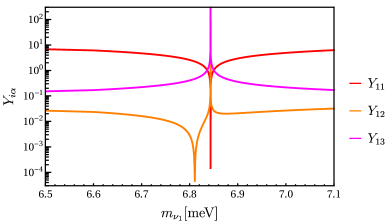
Figure 12: To the left, the entries of the first row of the Yukawa coupling matrix $Y$ zoomed around the poles for $Y_{11}$ and $Y_{12}$ for $\alpha_{12}=\alpha_{13}=\delta=\pi$. To the right, the calculated Br($l_{\alpha}\to l_{\beta}\gamma$). Both computed fixing ${\cal R}$ for $Y_{21}=Y_{31}=0$ and at the minimum allowed value of $m_{N}/F_{\rm AKS}$. While a pole for $Y_{11}$ exists, no pole for Br($\mu\rightarrow e\gamma$) or Br($\tau\rightarrow e\gamma$) is associated to it, due to the divergence of $Y_{12}$ and $Y_{13}$ on the pole. Note that only near the pole for $Y_{12}$ Br($\mu\rightarrow e\gamma$) is below the experimental limit.

In Fig. 12 to the left, we show the behavior of the first row of $Y$ for $\alpha_{12}=\alpha_{13}=\delta=\pi$. We considered for simplicity that all the scalar masses are equal to $m_{S^{+}}=m_{\varphi}=m_{\mathcal{H}^{\pm}}\equiv m_{S}$ and all the $N$ singlet fermion masses to be degenerate, $m_{N}$, and minimize $m_{N}/F_{\rm AKS}$ to find the lowest value of $Y$, see Eq. (46). We found this minimum for $m_{N}=272$ GeV and $m_{\mathcal{S}}=100$ GeV, where $F_{\rm AKS}\approx 0.44$, compatible with the limit on scalar masses from LEP [39]. Here we do not show the other four non-zero Yukawas for simplicity. They are nearly constant and of order $0.1$. Similar to the cocktail model (Fig. 2), poles exist in the different Yukawa entries for particular values of the phases and $m_{\nu_{1}}$. The main difference lies in the divergence that appears when $Y_{11}=0$. This is caused by our choice of ${\cal R}$ matrix, such that $Y_{21}=Y_{31}=0$. In this case, the pole in $Y_{11}$ does not imply a pole in Br($\mu\rightarrow e\gamma$) or Br($\tau\rightarrow e\gamma$), as it can be seen in Fig. 12 to the right. In fact, the product of $|Y_{11}Y_{13}^{*}|$ remains constant over the pole and very close to the current experimental limit of $3.3\times 10^{-8}$ [67]. Only the region around the pole in $Y_{12}$ is allowed by the experimental limit Br($\mu\rightarrow e\gamma$)$<4.2\times 10^{-13}$ [65].

To sum up, the parameter space of the AKS model is constrained mainly by perturbativity and Br($\mu\rightarrow e\gamma$). The former can be addressed with the freedom in ${\cal R}$ to set $Y_{21}$ and $Y_{31}$ to zero. As well as by fixing the Majorana and Dirac phases, and the lightest neutrino mass, to be near the pole of $Y_{11}$, where its value is lower than $4\pi$. On the other hand, to be below the experimental limit on Br($\mu\rightarrow e\gamma$), a similar fine-tuning of the phases and $m_{\nu_{1}}$ should be done to be around the narrow pole of $Y_{12}$. The parameter space is then restricted to those values of the phases and $m_{\nu_{1}}$ where the poles of $Y_{11}$ and $Y_{12}$ exist, and they are close enough to each other to avoid the limit on Br($\mu\rightarrow e\gamma$) while $Y_{11}$ is still perturbative.

Figure 13: Br($\mu\rightarrow e\gamma$) scanned over neutrino oscillation data in $1\sigma$ (light blue) and $3\sigma$ (dark blue) ranges. This plot scans over the Majorana phases. The shaded gray area corresponds to the most conservative limit to non-perturbative Yukawas.

In Fig. 13 we show the value of Br($\mu\rightarrow e\gamma$) scanning over the complete range of oscillation parameters (NH) and phases. On the right, we give the limit due to perturbativity of $Y_{11}$, reducing the parameter space to a small window of $m_{\nu_{1}}=(4.5-20)$ meV. Note that like in the cocktail model, $Y_{11}$ behaves as $m_{ee}$, and for $m_{\nu_{1}}\raise 1.29167pt\hbox{$\;>$\kern-7.5pt\raise-4.73611pt\hbox{$\sim\;$}}10$ meV, $m_{ee}$ has no pole, so $Y_{11}$ is in the non-perturbative region. Moreover, the cancellation of $Y_{11}$ and $Y_{12}$ only occurs for NH, so the model can only explain neutrino data with this neutrino mass ordering. In the following, we shall consider only NH.

Fig. 13 not only implies a constraint on $m_{\nu_{1}}$, but also on the phases. In Fig. 14 we show the points allowed by perturbativity and the experimental limits on Br($\mu\rightarrow e\gamma$), Br($\tau\rightarrow e\gamma$) and Br($\tau\rightarrow\mu\gamma$), for the values of the three phases. We scanned over the phases and masses, with $m_{S}>100$ GeV, allowing oscillation data to vary in $3\sigma$. As it can be seen, $\alpha_{12}$ should be closely around $\pi$, while $\delta$ is constrained to values between roughly $\pi/2$ and $3\pi/2$. For $\delta$ outside this window, there is no cancellation of $Y_{12}$. In the following, we restrict the results shown to the region where Br($\mu\rightarrow e\gamma$)$<4.2\times 10^{-13}$.

Figure 14: Allowed parameter space for $\alpha_{12}$, $\alpha_{13}$ and $\delta$. Neutrino oscillation data was scanned over the $3\sigma$ uncertainties, except $\delta$ which was left free. For points outside this region, either $Y_{11}$ is non-perturbative or Br($\mu\rightarrow e\gamma$) is above the experimental limit.

Now we move to analyse $\tau\to e\gamma$ and $\tau\rightarrow\mu\gamma$. As shown in Fig. 12 (right), while Br($\tau\rightarrow\mu\gamma$) is below the experimental limit, except on the pole of $Y_{11}$, Br($\tau\rightarrow e\gamma$) is mainly constant and close to the experimental limit. In Fig. 15 we give both branching ratios fixing $\delta$ to the b.f.p. and scanning over the uncertainties in the rest of the oscillation parameters. We consider $(m_{N}/F_{\rm AKS})_{min}$ with $m_{S}=100$ GeV and $m_{N}=272$ GeV. Points colored in gray correspond to non-perturbative Yukawas. We see that while Br($\tau\rightarrow\mu\gamma$) is safe, the allowed region on the left plot is severely constrained by the experimental limit Br($\tau\rightarrow e\gamma$)$<3.3\times 10^{-8}$. This tension can be mitigated by raising the masses, see Fig. 16. For the AKS model, the dominant contribution to Br($l_{\alpha}\to l_{\beta}\gamma$) is approximately proportional to $1/M^{4}$, with $M$ the dominant scale [68]. On the other hand, $m_{N}/F_{\rm AKS}$ is minimal for masses around $m_{S}=100$ GeV and $m_{N}=272$ GeV. So for masses away from these values, $m_{N}/F_{\rm AKS}$ increases and, consequently, the absolute scale of the Yukawas increases as well (see Eq. (46)), hence narrowing the region where the Yukawas are perturbative. For $m_{N}(m_{S^{+}})\sim 10^{6}$ GeV, we found no points allowed by perturbativity and the experimental limit on Br($\mu\rightarrow e\gamma$). In Fig. 16, in order to minimize the Yukawas, we fixed $m_{\varphi}=m_{\mathcal{H}^{\pm}}=100$ GeV and change $m_{S^{+}}$ and $m_{N}$, which enter in the calculation of Br($l_{\alpha}\to l_{\beta}\gamma$).

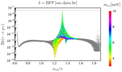
Figure 15: Br($\tau\rightarrow e\gamma$) and Br($\tau\rightarrow\mu\gamma$) as functions of $\alpha_{13}$ for different values of the lightest neutrino mass (color-coded) along with the current experimental limits (dotted line). We scanned over $3\sigma$ uncertainties of the oscillation data, except for $\delta$ which was fixed to the b.f.p. Gray points are excluded due to perturbativity arguments.

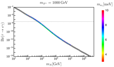
Figure 16: Calculated values for Br($\tau\rightarrow e\gamma$) as function of $m_{N}$ for different values of $m_{S^{+}}$. Here, we are maximizing the allowed parameter space in terms of $\alpha_{13}$. For the gray points, at least one entry in $Y$ is larger than $4\pi$.

A similar analysis can be done scanning over the Majorana phases too. Fig. 17 shows Br($\tau\rightarrow e\gamma$) as a function of $\alpha_{13}$ for different fermion and scalar masses. The allowed parameter space is bigger for $m_{N}$ around $272$ GeV, where $m_{N}/F_{\rm AKS}$ is minimal. For different masses the parameter space narrows, because $m_{N}/F_{\rm AKS}$ increases, as explained before. The upper limit is due to the phenomenological limit $m_{S^{+}}>100$ GeV, as for $m_{N}\ll m_{S^{+}}$, Br($\tau\rightarrow e\gamma$) is dominated by $m_{S^{+}}$. On the other side, while going to larger $m_{N}$ reduces considerably Br($\tau\rightarrow e\gamma$), a lower limit always exists due to perturbativity.

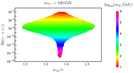
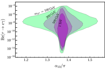
Figure 17: Br($\tau\rightarrow e\gamma$) for different values of $m_{N}$ and $m_{S^{+}}$. To the left, we fixed $m_{S^{+}}$ and see how by modifying $m_{N}$ the parameter space widens or narrows due to perturbativity arguments. A similar behavior can be observed for the plot on the right, where we show contour lines for different values of $m_{S^{+}}$ scanning over $m_{N}$.

We close this discussion with a short comment on $0\nu\beta\beta$ decay. There is no short-range diagram for $0\nu\beta\beta$ decay in the AKS model. Since, as discussed above, the AKS model survives only for normal hierarchy and in the part of parameter space where $m_{ee}$ is largely cancelled, observation of $0\nu\beta\beta$ decay in the next round of experiments would definitely rule out AKS as an explanation of neutrino masses.

6 Discussion

In this paper we have considered the cocktail, KNT and AKS models and studied their CLFV phenomenology. In these models, Majorana neutrino masses are generated at the 3-loop order, which naturally implies that large Yukawa couplings are required in order to reproduce the mass scales observed in neutrino oscillation experiments. As a result of this, perturbativity is typically lost. We have shown that one can decrease the Yukawa couplings by tuning some of the free parameters of these scenarios, such as the lightest neutrino mass $m_{\nu_{1}}$ or the Dirac and Majorana phases contained in the leptonic mixing matrix $U$. However, even after these parameters are tuned to recover perturbativity, the resulting CLFV branching ratios tend to largely exceed the existing bounds. In order to reduce the CLFV rates further tuning is needed. Our main conclusion is that the three models survive only in tiny correlated regions of their parameter spaces.

One should note that CLFV alone cannot exclude any of these models. The reason is that one can always reduce the CLFV rates as much as necessary by tuning the parameters of the model more finely. However, additional experimental handles exist. First, perturbativity imposes upper limits on the masses of some of the particles running in the loops. The reason is simple: larger mediator masses would imply a stronger suppression of the loop functions and then require larger Yukawa couplings. Thus, also future searches at the LHC in the high-luminosity phase would further restrict the available parameter space. An important experimental handle on the models is $0\nu\beta\beta$ decay. Since $m_{\nu_{1}}$ and the Majorana phases must be tuned for the models to survive, the effective $0\nu\beta\beta$ neutrino mass $m_{ee}$ becomes strongly constrained and definite predictions for the $0\nu\beta\beta$ rates are obtained for the AKS and KNT models. Any observation of $0\nu\beta\beta$ decay with the next generation of experiments would definitely rule out the AKS model. For the KNT model, because $m_{\nu_{1}}\simeq 0$, $m_{ee}$ has to be either in the range $m_{ee}\simeq(2-6)$ meV or $(15-50)$ meV for normal hierarchy or inverted hierarchy. Only the cocktail model is more flexible in its predictions for $0\nu\beta\beta$ decay, due to additional contributions from a sizable short-range diagram.

We mention also that only the KNT model can explain neutrino data for both hierarchies. Neither the cocktail nor the AKS model has any acceptable point in all of their parameter space in the case of inverse hierarchy.

A crucial ingredient in our analysis is the allowed size for the quartic scalar potential couplings that play a role in the neutrino mass generation mechanism, for example $\lambda_{5}$ in the cocktail model, $\lambda_{S}$ in the KNT model and $\kappa$ in the AKS model. Since neutrino masses are proportional to (some power of) these couplings, the larger they are, the smaller the Yukawa couplings can be. In our analysis, scalar couplings as large as $4\pi$ have been allowed. A more restrictive choice, with couplings at most of $\mathcal{O}(1)$, would alter the conclusions dramatically. In fact, all three models would already be ruled out, if all their couplings are restricted to be not larger than $\mathcal{O}(1)$.

Finally, we emphasize again that our strong claims only apply to the three minimal models considered here. There are several ways to modify these models so that they can evade the perturbativity and flavor constraints. For instance, one can introduce new exotic states in order to get rid of the proportionality to the charged lepton masses, at the origin of the problems discussed in our paper. Also, one may enhance the contributions to the neutrino mass matrix by using colored states. Nevertheless, we also note that there may be many other 3-loop (or 4-loop) neutrino mass models with the same issues.

Appendix A Loop integrals

In this Appendix we discuss the calculation of the loop integrals in the cocktail, KNT and AKS models. Here, we derive the loop functions used in the previous sections. For their computation, we did not rely on approximations, but implemented the full integral numerically using pySecDec [69].

Moreover, all the integrals shown here, can be factorized in terms of five master integrals (see for example [70]), as normally done. Nevertheless, we decided not to do it, because there is still no analytical general solution to all the 3-loop master integrals and their factorization could lead to numerical precision issues. Note that these five master integrals have divergent parts, while the full integral is finite.

A.1 Cocktail model

To compute the dimensionless integral $F_{\rm Cocktail}$ in Eq. (19), we choose the Feynman-’t Hooft gauge $\xi=1$. In this gauge, the propagator of the $W_{\mu}$ boson has no momenta structure in the numerator, while the standard Goldstone $H^{+}$ contribution with a mass $m_{W}^{2}$ should be included. We decided to show the diagrams in the gauge basis to be able to identify the different contributions that enter in $F_{\rm Cocktail}$.

Figure 18: Dimension $5$ mass diagrams in the gauge basis. Note that given the chirality, the corresponding integral has two momenta in the numerator. This is denoted with $\not{\partial}$. When referring to these diagrams we will use the notation $\mathfrak{I}^{(5)}_{i}$ with $i=1,2$ following the order of the figures.

We identified $12$ different diagrams in the gauge basis with dimensions $5$, $7$ and $9$, see Figs. 18-20. All of them are proportional to the mass of the charged leptons squared and with two derivatives. Naively, one could expect that the dominant contribution comes from the dimension $5$ diagrams. However, as we are considering $4\pi$ couplings and lowering the new physics scale as much as possible, all $12$ diagrams could be in principle relevant.

Figure 19: Dimension $7$ mass diagrams in the gauge basis. $W_{\mu}$ couples with a derivative to the scalars, so every diagram has the same number of derivatives. We will use the notation $\mathfrak{I}^{(7)}_{i}$ with $i=1,4$ following the usual order from left to right and top to bottom.

Figure 20: Dimension $9$ mass diagrams in the Feynman-’t Hooft gauge. Denoted as $\mathfrak{I}^{(9)}_{i}$ with $i=1,6$ when required, following the standard ordering (left to right and top to bottom).

We shall show in detail how we derived the integral of the first diagram in Fig. 20 as an example, denoted as $\mathfrak{I}^{(9)}_{1}$, and give just the results for the rest. We chose this diagram as it gives a similar prefactor as in the original work [10]. After electroweak symmetry breaking (EWSB), we rotate the diagram to the mass basis, see Fig. 21. $H^{+}$ is the Goldstone boson associated to $W_{\mu}$, which appears explicitly with mass $m_{W}$ in the Feynman-’t Hooft gauge. $\mathcal{H}^{+}$ are the two mass eigenstates with eigenvalues $m_{+}^{2}$ coming form the mixing of $S^{+}$ and $\eta^{+}$,

$$\mathcal{M}^{2}_{\mathcal{H}^{+}}=\left(\begin{array}[]{cc}M_{S}^{2}+\frac{1}{2}\lambda_{SH}v^{2}&\frac{1}{\sqrt{2}}\mu_{1}v\\ \frac{1}{\sqrt{2}}\mu_{1}v&M_{\eta}^{2}+\frac{1}{2}\left(\lambda_{\eta H}^{(1)}+\lambda_{\eta H}^{(3)}\right)v^{2}\end{array}\right)\,,$$ (48)

which can be trivially diagonalized by a $2\times 2$ rotation matrix $R_{\mathcal{H}^{+}}$ with angle $\beta$. $\eta_{R,I}$ are the CP-even and CP-odd components of $\eta^{0}$, with masses $m_{R,I}^{2}=M_{\eta}^{2}\mp\frac{1}{2}\lambda_{5}v^{2}$.

Figure 21: Mass diagram after EWSB in the Feynman-’t Hooft gauge. $H^{+}$ is the Goldstone boson associated to $W_{\mu}$ with mass $m_{W}$.

Defining $\int_{k}\equiv(16\pi^{2})\int d^{4}k/(2\pi)^{3}$ and assigning momenta in the loop, the integral of the diagram in Fig. 21 in the mass insertion approximation is given by

$$\mathcal{I}^{(9)}_{1}=(R_{\mathcal{H}^{+}})_{1i}(R_{\mathcal{H}^{+}})_{2i}(R_{\mathcal{H}^{+}})_{1j}(R_{\mathcal{H}^{+}})_{2j}\,\,\,\times\\ \medmath{\iiint\limits_{k_{1}\,k_{2}\,k_{3}}\,\frac{k_{1}\cdot k_{2}}{(k_{1}^{2})(k_{2}^{2})(k_{1}^{2}+m_{W}^{2})(k_{2}^{2}+m_{W}^{2})((k_{1}+k_{2})^{2}+m_{\rho^{++}}^{2})(k_{3}^{2}+m_{a}^{2})((k_{1}+k_{3})^{2}+m_{+i}^{2})((k_{2}-k_{3})^{2}+m_{+j}^{2})}}\,,$$ (49)

where $a=R,I$ and we have neglected the masses of the charged SM fermions. The sum over free indices can be explicitly done enlarging the denominator of the integral. For example,

$$\sum_{a=1}^{2}\frac{1}{k^{2}-m_{a}^{2}}=(m_{1}^{2}-m_{2}^{2})\frac{1}{(k^{2}-m_{1}^{2})(k^{2}-m_{2}^{2})}\,.$$ (50)

Defining $\Delta m_{0}^{2}=m_{R}^{2}-m_{I}^{2}$ and $\Delta m_{+}^{2}=m_{+1}^{2}-m_{+2}^{2}$, Eq. (49) can be written as,

$$\mathcal{I}^{(9)}_{1}=\frac{1}{4}\sin^{2}\!2\beta\,\Delta m_{0}^{2}\,(\Delta m_{+}^{2})^{2}\frac{1}{m_{\rho^{++}}^{8}}\,\widehat{\mathcal{I}}^{(1)}_{1}\,,$$ (51)

with $\widehat{\mathcal{I}}^{(1)}_{1}$ a dimensionless integral defined in Eq. (67), which depends only on mass ratios with $m_{\rho^{++}}$,

$$x_{W}=\frac{m_{W}^{2}}{m_{\rho^{++}}^{2}},\quad x_{R}=\frac{m_{R}^{2}}{m_{\rho^{++}}^{2}},\quad x_{I}=\frac{m_{I}^{2}}{m_{\rho^{++}}^{2}},\quad x_{1}=\frac{m_{+1}^{2}}{m_{\rho^{++}}^{2}},\quad x_{2}=\frac{m_{+2}^{2}}{m_{\rho^{++}}^{2}}\,.$$ (52)

Finally, including the corresponding couplings from the potential Eq. (3.1), the expression for the diagram in Fig. 21 reads

$$\mathfrak{I}^{(9)}_{1}=\frac{1}{4}{\lambda_{\eta H}^{(3)}}^{2}\,\sin^{2}\!2\beta\,\frac{\mu_{2}\,\Delta m_{0}^{2}\,(\Delta m_{+}^{2})^{2}}{m_{\rho^{++}}^{8}}\,\widehat{\mathcal{I}}^{(1)}_{1}\,,$$ (53)

where the Yukawa $h$ and the SM charged fermion masses have been omitted.

The computation of the rest of the diagrams in Figs. 18-20 is very similar to the example shown. We only give the results here and omit their calculation. The function $F_{\rm Cocktail}$ in Eq. (19) is given by the sum of the different contributions from the diagrams, i.e.

$$F_{\rm Cocktail}=\frac{m_{\rho^{++}}}{\lambda_{5}}\sum_{d,i}\,\mathfrak{I}^{(d)}_{i}\,,$$ (54)

with $d=5,7,9$ using the notation in Figs. 18-20. The prefactor originates from the normalization of Eq. (19). The corresponding $12$ contributions from each diagram are

$$\mathfrak{I}^{(5)}_{1} = 2\,\frac{\mu_{1}^{2}\,\mu_{2}\,\Delta m_{0}^{2}}{v^{2}m_{\rho^{++}}^{4}}\left[\cos^{4}\!\beta\,\frac{(\Delta m_{+}^{2})^{2}}{m_{\rho^{++}}^{4}}\,\widehat{\mathcal{I}}^{(1)}_{1}\,+2\cos 2\beta\,\frac{\Delta m_{+}^{2}}{m_{\rho^{++}}^{2}}\,\widehat{\mathcal{I}}^{(1)}_{2}\,+\,\widehat{\mathcal{I}}^{(1)}_{3}\right],$$ (55)

$$\mathfrak{I}^{(5)}_{2} = 4\,\kappa\,\frac{\mu_{1}\,\Delta m_{0}^{2}}{v^{2}m_{\rho^{++}}^{2}}\left[\cos^{2}\!\beta\,\frac{\Delta m_{+}^{2}}{m_{\rho^{++}}^{2}}\,\widehat{\mathcal{I}}^{(1)}_{4}\,+\,\widehat{\mathcal{I}}^{(1)}_{5}\right],$$ (56)

$$\mathfrak{I}^{(7)}_{1} = \sqrt{2}\,\lambda_{\eta H}^{(3)}\,\frac{\mu_{1}\,\mu_{2}\,\Delta m_{0}^{2}\,\Delta m_{+}^{2}}{v\,m_{\rho^{++}}^{6}}\,\sin\!2\beta\,\left[\cos\!\beta\,\sin\!2\beta\,\frac{\Delta m_{+}^{2}}{m_{\rho^{++}}^{2}}\,\widehat{\mathcal{I}}^{(1)}_{1}\,+\,\widehat{\mathcal{I}}^{(1)}_{2}\right],$$ (57)

$$\mathfrak{I}^{(7)}_{2} = -\frac{1}{2}\,g_{2}^{2}\,\frac{\mu_{1}\,\mu_{2}\,\Delta m_{0}^{2}\,\Delta m_{+}^{2}}{v\,m_{\rho^{++}}^{6}}\,\sin\!2\beta\,\left[\cos\!\beta\,\sin\!2\beta\,\frac{\Delta m_{+}^{2}}{m_{\rho^{++}}^{2}}\,\widehat{\mathcal{I}}^{(1)}_{1}\,+\,\widehat{\mathcal{I}}^{(1)}_{2}\right],$$ (58)

$$\mathfrak{I}^{(7)}_{3} = \sqrt{2}\,\lambda_{\eta H}^{(3)}\,\kappa\,\frac{\Delta m_{0}^{2}\,\Delta m_{+}^{2}}{v\,m_{\rho^{++}}^{4}}\,\sin 2\beta\,\widehat{\mathcal{I}}^{(1)}_{4}\,,$$ (59)

$$\mathfrak{I}^{(7)}_{4} = -\frac{1}{2}\,g_{2}^{2}\,\kappa\,\frac{\Delta m_{0}^{2}\,\Delta m_{+}^{2}}{v\,m_{\rho^{++}}^{4}}\,\sin 2\beta\,\widehat{\mathcal{I}}^{(2)}_{4}\,,$$ (60)

$$\mathfrak{I}^{(9)}_{1} = \frac{1}{4}{\lambda_{\eta H}^{(3)}}^{2}\,\frac{\mu_{2}\,\Delta m_{0}^{2}\,(\Delta m_{+}^{2})^{2}}{m_{\rho^{++}}^{8}}\,\sin^{2}\!2\beta\,\widehat{\mathcal{I}}^{(1)}_{1}\,,$$ (61)

$$\mathfrak{I}^{(9)}_{2} = -\frac{1}{4\sqrt{2}}\,g_{2}^{2}\,\lambda_{\eta H}^{(3)}\,\frac{\mu_{2}\,\Delta m_{0}^{2}\,(\Delta m_{+}^{2})^{2}}{m_{\rho^{++}}^{8}}\,\sin^{2}\!2\beta\,\widehat{\mathcal{I}}^{(2)}_{1}\,,$$ (62)

$$\mathfrak{I}^{(9)}_{3} = \frac{1}{32}\,g_{2}^{4}\,\frac{\mu_{2}\,\Delta m_{0}^{2}\,(\Delta m_{+}^{2})^{2}}{m_{\rho^{++}}^{8}}\,\sin^{2}\!2\beta\,\widehat{\mathcal{I}}^{(3)}_{1}\,,$$ (63)

$$\mathfrak{I}^{(9)}_{4} = -\frac{1}{\sqrt{2}}\,{\lambda_{\eta H}^{(3)}}^{2}\,\kappa\,\frac{v\,\Delta m_{0}^{2}\,\Delta m_{+}^{2}}{m_{\rho^{++}}^{6}}\,\sin\!2\beta\,\left[\cos\!\beta\,\sin\!2\beta\,\frac{\Delta m_{+}^{2}}{m_{\rho^{++}}^{2}}\,\widehat{\mathcal{I}}^{(1)}_{1}\,+\,\widehat{\mathcal{I}}^{(1)}_{2}\right],$$ (64)

$$\mathfrak{I}^{(9)}_{5} = \frac{1}{4}\,g_{2}^{2}\,\lambda_{\eta H}^{(3)}\,\kappa\,\frac{v\,\Delta m_{0}^{2}\,\Delta m_{+}^{2}}{m_{\rho^{++}}^{6}}\,\sin\!2\beta\,\left[\cos\!\beta\,\sin\!2\beta\,\frac{\Delta m_{+}^{2}}{m_{\rho^{++}}^{2}}\,\widehat{\mathcal{I}}^{(1)}_{1}\,+\,\widehat{\mathcal{I}}^{(1)}_{2}\right],$$ (65)

$$\mathfrak{I}^{(9)}_{6} = -\frac{1}{4\sqrt{2}}\,g_{2}^{4}\,\kappa\,\frac{v\,\Delta m_{0}^{2}\,\Delta m_{+}^{2}}{m_{\rho^{++}}^{6}}\,\sin\!2\beta\,\left[\cos\!\beta\,\sin\!2\beta\,\frac{\Delta m_{+}^{2}}{m_{\rho^{++}}^{2}}\,\widehat{\mathcal{I}}^{(1)}_{1}\,+\,\widehat{\mathcal{I}}^{(1)}_{2}\right],$$ (66)

For simplicity we introduced the notation

$$\widehat{\mathcal{I}}^{(a)}_{i}=\iiint\limits_{k_{1}\,k_{2}\,k_{3}}\,\frac{\mathcal{N}_{a}}{\mathcal{D}_{i}}\,,$$ (67)

where each numerator, associated to the derivatives depicted in the diagrams, is defined as

$$\mathcal{N}_{1} = k_{1}\cdot k_{2}\,,$$

$$\mathcal{N}_{2} = k_{2}\cdot(2k_{3}+k_{1})\,,$$ (68)

$$\mathcal{N}_{3} = (2k_{3}+k_{1})\cdot(2k_{3}+k_{2})\,,$$

while for the denominators,

$$\mathcal{D}_{0} = (k_{1}^{2})(k_{2}^{2})(k_{1}^{2}+x_{W})(k_{2}^{2}+x_{W})((k_{1}+k_{2})^{2}+1)(k_{3}^{2}+x_{R})(k_{3}^{2}+x_{I})\,,$$

$$\mathcal{D}_{1} = \mathcal{D}_{0}\times((k_{1}+k_{3})^{2}+x_{1})((k_{2}-k_{3})^{2}+x_{1})((k_{1}+k_{3})^{2}+x_{2})((k_{2}-k_{3})^{2}+x_{2})\,,$$

$$\mathcal{D}_{2} = \mathcal{D}_{0}\times((k_{1}+k_{3})^{2}+x_{1})((k_{1}+k_{3})^{2}+x_{2})((k_{2}-k_{3})^{2}+x_{2})\,,$$

$$\mathcal{D}_{3} = \mathcal{D}_{0}\times((k_{1}+k_{3})^{2}+x_{1})((k_{2}-k_{3})^{2}+x_{2})\,,$$ (69)

$$\mathcal{D}_{4} = \mathcal{D}_{0}\times((k_{2}-k_{3})^{2}+x_{1})((k_{2}-k_{3})^{2}+x_{2})\,,$$

$$\mathcal{D}_{5} = \mathcal{D}_{0}\times((k_{2}-k_{3})^{2}+x_{2})\,,$$

with the mass ratios $x$ defined in Eq. (52). The integrals in Eq. (67) are evaluated numerically using pySecDec.

We now discuss the maximization of $F_{\rm Cocktail}$. We are interested in this case, because the Yukawa $h$ in Eq. (22) is inversely proportional to $F_{\rm Cocktail}$, and we want to explore the parameter space where $h$ is small enough to be perturbative and avoid CLFV constraints. In general, every integral $\widehat{\mathcal{I}}^{(a)}_{i}$ gets larger for smaller masses or, equivalently, smaller ratios. We shall fix a limit of $100$ GeV on the scalar masses of $\eta_{R,I}$ and $\mathcal{H}^{+}$, and $800$ GeV for the doubly charged singlet $\rho^{++}$, see Sec. 3 for details. We set the dimensionless couplings $\lambda_{5}$, $\lambda_{\eta H}^{(3)}$, and $\kappa$ to $4\pi$. For the dimensionful $\mu$ couplings we impose the limits $\mu_{1}<4\,\text{max}[m_{+1},m_{+2}]$ and $\mu_{2}<4\,\text{max}[m_{+1},m_{+2},m_{\rho^{++}}]$, required to avoid the radiative generation of negative quartic scalar couplings [51].

We found the maximum value of $F_{\rm Cocktail}^{\rm max}\simeq 192$ for $m_{R}=m_{+1}=100$ GeV, $m_{\rho^{++}}=800$ GeV, $m_{I}=878$ GeV, and $m_{+2}=1237$ GeV, with maximal mixing angle $\beta=\pi/4$. $\mu_{1}=(\Delta m_{+}^{2})/\sqrt{2}v=4372$ GeV, while $\mu_{2}$ is simply $4\,m_{+2}$.

A.2 KNT model

Figure 22: Neutrino mass diagram for the KNT model in the gauge basis.

The computation of the mass diagram for the KNT model is much simpler than the one in the cocktail model. The main contribution to the neutrino mass comes only from the diagram in Fig. 22 in the electroweak symmetric basis. Moreover, there is no mixing between the scalars participating in the loop, so $F_{\rm KNT}$ in Eq. (29) is just the 3-loop integral of the diagram in the mass basis shown in Fig. 6. Neglecting the SM charged fermion masses, one finds

$$F_{\rm KNT}=\iiint\limits_{k_{1}\,k_{2}\,k_{3}}\frac{1}{(k_{1}^{2})(k_{2}^{2})(k_{1}^{2}+x_{1})(k_{2}^{2}+x_{1})(k_{3}^{2}+1)((k_{1}-k_{3})^{2}+x_{2})((k_{2}-k_{3})^{2}+x_{2})}\,,$$ (70)

which is a dimensionless function of the ratios,

$$x_{1}=\frac{m_{s_{1}}^{2}}{M_{N_{i}}^{2}}\,,\quad x_{2}=\frac{m_{s_{2}}^{2}}{M_{N_{i}}^{2}}\,.$$ (71)

Note that Eq. (70) is simple enough to be easily decomposed in terms of 3-loop master integrals [70]. Due to the repetitions of the momenta in the denominator, using relation (22) from [8], one has

$$F_{\rm KNT}=\iiint\limits_{k_{1}\,k_{2}\,k_{3}}\frac{1}{(k_{3}^{2}-1)((k_{1}-k_{3})^{2}-x_{2})((k_{2}-k_{3})^{2}-x_{2})}\,\,\times\\ \frac{1}{x_{1}}\left[\frac{1}{(k_{1}^{2}-x_{1})(k_{2}^{2}-x_{1})}-\frac{1}{(k_{1}^{2})(k_{2}^{2}-x_{1})}-\frac{1}{(k_{1}^{2}-x_{1})(k_{2}^{2})}+\frac{1}{(k_{1}^{2})(k_{2}^{2})}\right].$$ (72)

As the second and third terms are identical under the exchange of $k_{1}$ and $k_{2}$, one can finally write $F_{\rm KNT}$ in terms of a combination of the master integral $\mathbf{G}$ integral given in [70]. The resulting expression is

$$F_{\rm KNT}=\frac{1}{x_{1}}\left[\mathbf{G}(1,x_{1},x_{2},x_{1},x_{2})-2\,\mathbf{G}(1,x_{1},x_{2},0,x_{2})+\mathbf{G}(1,0,x_{2},0,x_{2})\right].$$ (73)

The integral has an analytical expression for $x_{1i}=x_{2i}=1$.

About the maximum value of $F_{\rm KNT}$, we proceeded analogously to the cocktail model. In this case, we maximized $F_{\rm KNT}/M_{N_{i}}$, since the neutrino mass matrix in Eq. (29) is proportional to this ratio. We set a lower limit on the mass of the singly charged scalars of $100$ GeV and let $M_{N_{i}}=M_{N}$ free. We found that the maximum is around $F_{\rm KNT}\simeq 60$ with $m_{S_{1}}=m_{S_{2}}=100$ GeV and $M_{N_{i}}=840$ GeV.

A.3 AKS model

Figure 23: Neutrino mass diagrams for the AKS model in the gauge basis.

In this case, there exists two non-equivalent diagrams shown in Fig. 23, which differ by the crossing of the internal $S$-lines. $F_{\rm AKS}$ is then the sum of the integrals from both diagrams with the correct normalization, given in Eq. (45),

$$F_{\rm AKS}=\mathfrak{I}_{1}\,+\,\mathfrak{I}_{2}\,.$$ (74)

By assigning momenta to the internal fields, the two dimensionless integrals can be compactly expressed as,

$$\mathfrak{I}_{i}=\iiint\limits_{k_{1}\,k_{2}\,k_{3}}\frac{k_{1}\cdot k_{2}}{\mathcal{D}_{i}}\,,$$ (75)

with the denominators,

$$\mathcal{D}_{0} = (k_{1}^{2})(k_{1}^{2}-x_{1})(k_{2}^{2})(k_{2}^{2}-x_{1})(k_{3}^{2}-1)((k_{1}-k_{3})^{2}-x_{S})((k_{2}+k_{3})^{2}-x_{S})\,,$$

$$\mathcal{D}_{1} = \mathcal{D}_{0}\,\times\,(k_{3}^{2}-x_{\varphi})\,,$$ (76)

$$\mathcal{D}_{2} = \mathcal{D}_{0}\,\times\,((k1+k_{2}+k_{3})^{2}-x_{\varphi})\,,$$

where we have neglected the SM charged fermion masses. The ratios of masses are then defined as

$$x_{1}=\frac{m_{\mathcal{H}}^{2}}{M_{N_{i}}^{2}}\,,\quad x_{\varphi}=\frac{m_{\varphi}^{2}}{M_{N_{i}}^{2}}\,,\quad x_{S}=\frac{m_{S^{+}}^{2}}{M_{N_{i}}^{2}}\,.$$ (77)

Similar to the previous models, we computed the maximum of the function $F_{\rm AKS}/M_{N_{i}}$ to minimize the absolute scale of the Yukawa $Y$. We considered $M_{N_{i}}=m_{N}$ and set a lower limit of $100$ GeV to the scalar masses. We found the maximum for $m_{N}=272$ GeV and $m_{\mathcal{H}}=m_{\varphi}=m_{S}=100$ GeV where $F_{\rm AKS}\simeq 0.45$.

References

- [1] A. Zee, “A theory of lepton number violation, neutrino Majorana mass, and oscillation,” Phys.Lett. B93 (1980) 389.
- [2] T. P. Cheng and L.-F. Li, “Neutrino masses, mixings and oscillations in models of electroweak interactions,” Phys. Rev. D22 (1980) 2860.
- [3] A. Zee, “Quantum numbers of Majorana neutrino masses,” Nucl. Phys. B264 (1986) 99–110.
- [4] K. S. Babu, “Model of “calculable” Majorana neutrino masses,” Phys. Lett. B203 (1988) 132–136.
- [5] F. Bonnet, M. Hirsch, T. Ota, and W. Winter, “Systematic study of the d=5 Weinberg operator at one-loop order,” JHEP 07 (2012) 153, arXiv:1204.5862 [hep-ph].
- [6] D. Aristizabal Sierra, A. Degee, L. Dorame, and M. Hirsch, “Systematic classification of two-loop realizations of the Weinberg operator,” JHEP 03 (2015) 040, arXiv:1411.7038 [hep-ph].
- [7] R. Cepedello, R. Fonseca, and M. Hirsch, “Neutrino masses beyond the minimal seesaw,” in 16th International Conference on Topics in Astroparticle and Underground Physics (TAUP 2019) Toyama, Japan, September 9-13, 2019. 2019. arXiv:1911.01125 [hep-ph].
- [8] R. Cepedello, R. M. Fonseca, and M. Hirsch, “Systematic classification of three-loop realizations of the Weinberg operator,” JHEP 10 (2018) 197, arXiv:1807.00629 [hep-ph]. [erratum: JHEP06,034(2019)].
- [9] Y. Cai, J. Herrero-García, M. A. Schmidt, A. Vicente, and R. R. Volkas, “From the trees to the forest: a review of radiative neutrino mass models,” Front.in Phys. 5 (2017) 63, arXiv:1706.08524 [hep-ph].
- [10] M. Gustafsson, J. M. No, and M. A. Rivera, “Predictive Model for Radiatively Induced Neutrino Masses and Mixings with Dark Matter,” Phys. Rev. Lett. 110 no. 21, (2013) 211802, arXiv:1212.4806 [hep-ph]. [Erratum: Phys. Rev. Lett.112,no.25,259902(2014)].
- [11] L. M. Krauss, S. Nasri, and M. Trodden, “A Model for neutrino masses and dark matter,” Phys. Rev. D67 (2003) 085002, arXiv:hep-ph/0210389 [hep-ph].
- [12] M. Aoki, S. Kanemura, and O. Seto, “Neutrino mass, Dark Matter and Baryon Asymmetry via TeV-Scale Physics without Fine-Tuning,” Phys. Rev. Lett. 102 (2009) 051805, arXiv:0807.0361 [hep-ph].
- [13] C.-Q. Geng, D. Huang, and L.-H. Tsai, “Loop-induced Neutrino Masses: A Case Study,” Phys. Rev. D90 no. 11, (2014) 113005, arXiv:1410.7606 [hep-ph].
- [14] Y. Kajiyama, H. Okada, and K. Yagyu, “ Flavor Model in Three Loop Seesaw and Higgs Phenomenology,” JHEP 10 (2013) 196, arXiv:1307.0480 [hep-ph].
- [15] H. Hatanaka, K. Nishiwaki, H. Okada, and Y. Orikasa, “A Three-Loop Neutrino Model with Global Symmetry,” Nucl. Phys. B894 (2015) 268–283, arXiv:1412.8664 [hep-ph].
- [16] J. Alcaide, D. Das, and A. Santamaria, “A model of neutrino mass and dark matter with large neutrinoless double beta decay,” JHEP 04 (2017) 049, arXiv:1701.01402 [hep-ph].
- [17] M. Aoki, S. Kanemura, and O. Seto, “A model of TeV scale physics for neutrino mass, dark matter and baryon asymmetry and its phenomenology,” Phys. Rev. D80 (2009) 033007, arXiv:0904.3829 [hep-ph].
- [18] M. Aoki, S. Kanemura, and O. Seto, “ILC phenomenology in a TeV scale radiative seesaw model for neutrino mass, dark matter and baryon asymmetry,” in 8th General Meeting of the ILC Physics Subgroup Tsukuba, Japan, January 21, 2009. 2010. arXiv:1008.2407 [hep-ph]. http://inspirehep.net/record/865435/files/arXiv:1008.2407.pdf.
- [19] M. Aoki, S. Kanemura, and K. Yagyu, “Triviality and vacuum stability bounds in the three-loop neutrino mass model,” Phys. Rev. D83 (2011) 075016, arXiv:1102.3412 [hep-ph].
- [20] H. Okada and K. Yagyu, “Three-loop neutrino mass model with doubly charged particles from isodoublets,” Phys. Rev. D93 no. 1, (2016) 013004, arXiv:1508.01046 [hep-ph].
- [21] P.-H. Gu, “High-scale leptogenesis with three-loop neutrino mass generation and dark matter,” JHEP 04 (2017) 159, arXiv:1611.03256 [hep-ph].
- [22] S.-Y. Ho, T. Toma, and K. Tsumura, “Systematic extensions of loop-induced neutrino mass models with dark matter,” Phys. Rev. D94 no. 3, (2016) 033007, arXiv:1604.07894 [hep-ph].
- [23] K. Cheung and O. Seto, “Phenomenology of TeV right-handed neutrino and the dark matter model,” Phys. Rev. D69 (2004) 113009, arXiv:hep-ph/0403003 [hep-ph].
- [24] A. Ahriche, C.-S. Chen, K. L. McDonald, and S. Nasri, “Three-loop model of neutrino mass with dark matter,” Phys. Rev. D90 (2014) 015024, arXiv:1404.2696 [hep-ph].
- [25] A. Ahriche, K. L. McDonald, and S. Nasri, “A Model of radiative neutrino mass: with or without dark matter,” JHEP 10 (2014) 167, arXiv:1404.5917 [hep-ph].
- [26] A. Ahriche, K. L. McDonald, and S. Nasri, “A radiative model for the weak scale and neutrino mass via dark matter,” JHEP 02 (2016) 038, arXiv:1508.02607 [hep-ph].
- [27] A. Ahriche, K. L. McDonald, and S. Nasri, “Scalar sector phenomenology of three-loop radiative neutrino mMass models,” Phys. Rev. D92 no. 9, (2015) 095020, arXiv:1508.05881 [hep-ph].
- [28] A. Ahriche, K. L. McDonald, and S. Nasri, “Three-loop neutrino mass models at colliders,” in Proceedings, 50th Rencontres de Moriond Electroweak Interactions and Unified Theories: La Thuile, Italy, March 14-21, 2015, pp. 285–290. 2015. arXiv:1505.04320 [hep-ph]. http://inspirehep.net/record/1370679/files/arXiv:1505.04320.pdf.
- [29] A. Ahriche, S. Nasri, and R. Soualah, “Radiative neutrino mass model at the linear collider,” Phys. Rev. D89 no. 9, (2014) 095010, arXiv:1403.5694 [hep-ph].
- [30] A. Ahriche, K. L. McDonald, S. Nasri, and T. Toma, “A model of neutrino mass and dark matter with an accidental symmetry,” Phys. Lett. B746 (2015) 430–435, arXiv:1504.05755 [hep-ph].
- [31] P.-H. Gu, “From dark matter to neutrinoless double beta decay,” arXiv:1203.4165 [hep-ph].
- [32] T. Nomura, H. Okada, and N. Okada, “A Colored KNT neutrino model,” Phys. Lett. B762 (2016) 409–414, arXiv:1608.02694 [hep-ph].
- [33] K. Cheung, T. Nomura, and H. Okada, “Three-loop neutrino mass model with a colored triplet scalar,” Phys. Rev. D95 no. 1, (2017) 015026, arXiv:1610.04986 [hep-ph].
- [34] C. Hati, G. Kumar, J. Orloff, and A. M. Teixeira, “Reconciling -decay anomalies with neutrino masses, dark matter and constraints from flavour violation,” arXiv:1806.10146 [hep-ph].
- [35] H. Okada and K. Yagyu, “Renormalizable model for neutrino mass, dark matter, muon and 750 GeV diphoton excess,” Phys. Lett. B756 (2016) 337–344, arXiv:1601.05038 [hep-ph].
- [36] J. N. Ng and A. de la Puente, “Top Quark as a Dark Portal and Neutrino Mass Generation,” Phys. Lett. B727 (2013) 204–210, arXiv:1307.2606 [hep-ph].
- [37] C.-S. Chen, K. L. McDonald, and S. Nasri, “A Class of Three-Loop Models with Neutrino Mass and Dark Matter,” Phys. Lett. B734 (2014) 388–393, arXiv:1404.6033 [hep-ph].
- [38] P. F. de Salas, D. V. Forero, C. A. Ternes, M. Tortola, and J. W. F. Valle, “Status of neutrino oscillations 2018: 3 hint for normal mass ordering and improved CP sensitivity,” Phys. Lett. B782 (2018) 633–640, arXiv:1708.01186 [hep-ph].
- [39] Particle Data Group Collaboration, M. Tanabashi et al., “Review of Particle Physics,” Phys. Rev. D98 no. 3, (2018) 030001.
- [40] E. Ma, “Verifiable radiative seesaw mechanism of neutrino mass and dark matter,” Phys. Rev. D73 (2006) 077301, arXiv:hep-ph/0601225 [hep-ph].
- [41] ATLAS Collaboration, M. Aaboud et al., “Search for doubly charged Higgs boson production in multi-lepton final states with the ATLAS detector using proton–proton collisions at ,” Eur. Phys. J. C78 no. 3, (2018) 199, arXiv:1710.09748 [hep-ex].
- [42] CMS Collaboration, C. Collaboration, “A search for doubly-charged Higgs boson production in three and four lepton final states at ,”.
- [43] ATLAS Collaboration, M. Aaboud et al., “Search for doubly charged scalar bosons decaying into same-sign boson pairs with the ATLAS detector,” Eur. Phys. J. C79 no. 1, (2019) 58, arXiv:1808.01899 [hep-ex].
- [44] KamLAND-Zen Collaboration, A. Gando et al., “Search for Majorana Neutrinos near the Inverted Mass Hierarchy Region with KamLAND-Zen,” Phys. Rev. Lett. 117 no. 8, (2016) 082503, arXiv:1605.02889 [hep-ex]. [Addendum: Phys. Rev. Lett.117,no.10,109903(2016)].
- [45] GERDA Collaboration, M. Agostini et al., “Improved Limit on Neutrinoless Double- Decay of 76Ge from GERDA Phase II,” Phys. Rev. Lett. 120 no. 13, (2018) 132503, arXiv:1803.11100 [nucl-ex].
- [46] Planck Collaboration, N. Aghanim et al., “Planck 2018 results. VI. Cosmological parameters,” arXiv:1807.06209 [astro-ph.CO].
- [47] SINDRUM Collaboration, U. Bellgardt et al., “Search for the Decay ,” Nucl. Phys. B 299 (1988) 1–6.
- [48] M. Gustafsson, J. M. No, and M. A. Rivera, “Radiative neutrino mass generation linked to neutrino mixing and neutrinoless double beta decay predictions,” Phys. Rev. D90 no. 1, (2014) 013012, arXiv:1402.0515 [hep-ph].
- [49] M. González, M. Hirsch, and S. G. Kovalenko, “QCD running in neutrinoless double beta decay: Short-range mechanisms,” Phys. Rev. D93 no. 1, (2016) 013017, arXiv:1511.03945 [hep-ph]. [erratum: Phys. Rev.D97,no.9,099907(2018)].
- [50] C. Arbeláez, M. González, S. Kovalenko, and M. Hirsch, “QCD-improved limits from neutrinoless double beta decay,” Phys. Rev. D96 no. 1, (2017) 015010, arXiv:1611.06095 [hep-ph].
- [51] K. Babu and C. Macesanu, “Two loop neutrino mass generation and its experimental consequences,” Phys. Rev. D 67 (2003) 073010, arXiv:hep-ph/0212058.
- [52] J. Herrero-Garcia, M. Nebot, N. Rius, and A. Santamaria, “The Zee–Babu model revisited in the light of new data,” Nucl. Phys. B 885 (2014) 542–570, arXiv:1402.4491 [hep-ph].
- [53] I. Cordero-Carrión, M. Hirsch, and A. Vicente, “Master Majorana neutrino mass parametrization,” Phys. Rev. D99 no. 7, (2019) 075019, arXiv:1812.03896 [hep-ph].
- [54] I. Cordero-Carrión, M. Hirsch, and A. Vicente, “General parametrization of Majorana neutrino mass models,” arXiv:1912.08858 [hep-ph].
- [55] J. A. Casas and A. Ibarra, “Oscillating neutrinos and ,” Nucl. Phys. B618 (2001) 171–204, arXiv:hep-ph/0103065 [hep-ph].
- [56] CMS Collaboration, A. M. Sirunyan et al., “Search for supersymmetric partners of electrons and muons in proton-proton collisions at 13 TeV,” Phys. Lett. B 790 (2019) 140–166, arXiv:1806.05264 [hep-ex].
- [57] ATLAS Collaboration, G. Aad et al., “Search for electroweak production of charginos and sleptons decaying into final states with two leptons and missing transverse momentum in TeV collisions using the ATLAS detector,” Eur. Phys. J. C 80 no. 2, (2020) 123, arXiv:1908.08215 [hep-ex].
- [58] F. Staub, “SARAH 3.2: Dirac Gauginos, UFO output, and more,” Comput. Phys. Commun. 184 (2013) 1792–1809, arXiv:1207.0906 [hep-ph].
- [59] F. Staub, “SARAH 4 : A tool for (not only SUSY) model builders,” Comput. Phys. Commun. 185 (2014) 1773–1790, arXiv:1309.7223 [hep-ph].
- [60] W. Porod, “SPheno, a program for calculating supersymmetric spectra, SUSY particle decays and SUSY particle production at e+ e- colliders,” Comput. Phys. Commun. 153 (2003) 275–315, arXiv:hep-ph/0301101 [hep-ph].
- [61] W. Porod and F. Staub, “SPheno 3.1: Extensions including flavour, CP-phases and models beyond the MSSM,” Comput. Phys. Commun. 183 (2012) 2458–2469, arXiv:1104.1573 [hep-ph].
- [62] J. Alwall, P. Demin, S. de Visscher, R. Frederix, M. Herquet, F. Maltoni, T. Plehn, D. L. Rainwater, and T. Stelzer, “MadGraph/MadEvent v4: The New Web Generation,” JHEP 09 (2007) 028, arXiv:0706.2334 [hep-ph].
- [63] J. Alwall, M. Herquet, F. Maltoni, O. Mattelaer, and T. Stelzer, “MadGraph 5 : Going Beyond,” JHEP 1106 (2011) 128, arXiv:1106.0522 [hep-ph].
- [64] J. Alwall, R. Frederix, S. Frixione, V. Hirschi, F. Maltoni, O. Mattelaer, H. S. Shao, T. Stelzer, P. Torrielli, and M. Zaro, “The automated computation of tree-level and next-to-leading order differential cross sections, and their matching to parton shower simulations,” JHEP 07 (2014) 079, arXiv:1405.0301 [hep-ph].
- [65] MEG Collaboration, A. Baldini et al., “Search for the lepton flavour violating decay with the full dataset of the MEG experiment,” Eur. Phys. J. C 76 no. 8, (2016) 434, arXiv:1605.05081 [hep-ex].
- [66] A. Baldini et al., “MEG Upgrade Proposal,” arXiv:1301.7225 [physics.ins-det].
- [67] BaBar Collaboration, B. Aubert et al., “Searches for Lepton Flavor Violation in the Decays and ,” Phys. Rev. Lett. 104 (2010) 021802, arXiv:0908.2381 [hep-ex].
- [68] L. Lavoura, “General formulae for ,” Eur. Phys. J. C 29 (2003) 191–195, arXiv:hep-ph/0302221.
- [69] S. Borowka, G. Heinrich, S. Jahn, S. P. Jones, M. Kerner, J. Schlenk, and T. Zirke, “pySecDec: a toolbox for the numerical evaluation of multi-scale integrals,” Comput. Phys. Commun. 222 (2018) 313–326, arXiv:1703.09692 [hep-ph].
- [70] S. P. Martin and D. G. Robertson, “Evaluation of the general 3-loop vacuum Feynman integral,” Phys. Rev. D95 no. 1, (2017) 016008, arXiv:1610.07720 [hep-ph].