1 Introduction

A central question of physics beyond the Standard Model (SM) is whether there is intermediate-scale physics between the electroweak and the Planck scales and how to possibly test it. It can be reasonably argued that the SM is an effective field theory, valid until some cut-off scale $\Lambda_{\rm SM}\leq M_{\rm Pl}=1.2\times 10^{19}$ GeV and that (disregarding the long-pursued naturalness argument of the electroweak scale) the new layer of physical reality might lie much above the TeV scale. This is actually suggested by the inner structure of the SM: flavour and CP violating observables have generically probed scales up to $\Lambda_{\rm SM}\gtrsim 10^{6}$ GeV, while light neutrino masses point to $\Lambda_{\rm SM}\lesssim 10^{14}$ GeV. At the same time, it is evident that the hypercharge structure of the SM fermions cries out for unification (letting aside the more mysterious origin of flavour). Left-Right symmetric theories [1, 2, 3, 4] provide a most natural route for addressing the origin of hypercharge and neutrino masses, passing through the Pati-Salam partial unification scheme [1] (which also provides a rationale for the quantization of electric charge) and ending up into one SM family plus a right-handed neutrino unified into a spinorial representation of SO(10) [5, 6]. Due to the fact that these groups have rank 5, they admit at least an intermediate breaking stage before landing on the SM gauge group, and in the case of Pati-Salam [7] and SO(10) [8, 9, 10] those are often predicted to lie in between $10^{6}$ GeV and $10^{14}$ GeV by (partial) gauge coupling unification. This picture would gain an additional value if such intermediate-scale physics would be connected to other open issues of the SM, most notably the baryon asymmetry of the Universe and Dark Matter (DM). The former is built-in in the form of thermal leptogenesis [11], which in its simplest realization would suggest $\Lambda_{\rm SM}\gtrsim 10^{9}$ GeV (see e.g. [12]), while DM is often a missing ingredient in minimal realizations of Left-Right symmetric theories (for an exception, see [13]). A natural possibility is then to impose a Peccei-Quinn (PQ) symmetry [14, 15] delivering an axion [16, 17], which provides at the same time an excellent DM candidate [18, 19, 20] and solves the strong CP problem. This choice is economical also in the following sense: $i)$ in SO(10) setups the PQ symmetry was often imposed for another reason, namely to enhance the predictivity of the renormalizable (non-supersymmetric) SO(10) Yukawa sector [21] and $ii)$ it is based on a coincidence of scales: the axion decay constant is in fact bounded from astrophysical and cosmological consideration within the range $10^{8}\ \text{GeV}\lesssim f_{a}\lesssim 10^{18}\ \text{GeV}$ (see [22] for updated limits).

The scenario above is both simple and elegant enough for it to be taken seriously. Given the fact that it was clearly envisioned around four decades ago by Mohapatra and Senjanović [23] in the context of SO(10), and often reconsidered in different ways and at different levels of depth [24, 25, 26, 27, 28, 29, 30, 31, 32, 33, 34, 35, 36, 37, 38, 39, 40, 41, 42], it is worth to spend few words on why again now and why the Pati-Salam axion.

From an experimental point of view, there are now better hopes to catch the axion tail of the story. Axion physics is in fact in a blooming phase with several new detection concepts which promise to open for explorations regions of parameter space which were thought unreachable until few years ago (for updated experimental reviews see [43, 44]). In particular, the possibility that the Grand Unified Theory (GUT) axion window could be completely covered by the axion DM experiments CASPEr-Electric [45, 46] and ABRACADABRA [47] has triggered a revival of studies of GUT$\times{\rm U}(1)_{\rm PQ}$ models, with the axion field residing in a non-singlet representation of the GUT group. In particular, Ref. [37] computed for the first time low-energy axion couplings in SO(10)$\times{\rm U}(1)_{\rm PQ}$ models and considered axion mass predictions in SO(10) models with up to two intermediate breaking stages. Ref. [48] considered instead a minimal non-renormalizable SU(5)$\times{\rm U}(1)_{\rm PQ}$ model based on a PQ extension of [49, 50], which due to its minimality allowed to obtain (via the three-loop gauge coupling unification analysis of [51]) a sharp prediction for the axion mass in the neV domain. Subsequently, Refs. [52, 53] considered axion mass predictions in other minimal renormalizable SU(5)$\times{\rm U}(1)_{\rm PQ}$ models. Some cosmological consequences of supersymmetric axion GUTs were considered instead in [54].

The study of the Pati-Salam axion considered in the present work has a twofold motivation. On the one hand, the Pati-Salam (partial) unification constraints are genuinely different from SO(10) ones, so their predictions can be in principle discerned from those of SO(10). For instance, while it is notoriously difficult to obtain a low-scale Left-Right symmetry breaking scale in SO(10), we will show that if the Pati-Salam group is broken at the Planck scale, the Left-Right symmetry breaking can be as low as 20 TeV (and even lower in the absence of the PQ). One the other hand, the Pati-Salam gauge group, which is half-way through SO(10), provides a simpler setup and for this reason it can be studied in quite some detail. For instance, although SO(10)$\times{\rm U}(1)_{\rm PQ}$ scalar potentials have been partially classified in [26], they have never been investigated in detail. In the present work we provide also a non-trivial step in that direction, by working out the scalar potential dynamics of a complex scalar adjoint of ${\rm SU}(4)_{\rm PS}$, which hosts the axion field as a phase, and whose vacuum expectation value (VEV) is simultaneously responsible for PQ and Pati-Salam breaking down to the Left-Right symmetric gauge group. This allows in turn to constrain the axion mass via a renormalization group (RG) analysis of (partial) gauge coupling unification in Pati-Salam.

The paper is structured as follows. In Sect. 2.1 we describe the logic behind the construction of a minimal renormalizable Pati-Salam$\times{\rm U}(1)_{\rm PQ}$ model. Next, we focus on axion couplings (Sect. 2.2) and on the axion mass prediction from Pati-Salam breaking (Sect. 2.3). This is the main conceptual point of the paper, which relies on the calculable relation between the axion mass and the Pati-Salam breaking scale (cf. Eq. (2.42)). The latter can then be constrained via a RG analysis of (partial) gauge coupling unification within the Pati-Salam model. In Sect. 2.4 we report the results of such RG analysis, which is based both on a one-loop analytical understanding and a more involved two-loop numerical investigation, whose details are deferred to App. A. The main outcome of the RG analysis is that the Pati-Salam breaking scale (the axion mass) becomes a decreasing (increasing) function of a sliding Left-Right symmetry breaking scale. Sect. 3 is devoted to the phenomenology of the model and to the experimental prospects for hunting the Pati-Salam axion. We first collect various cosmological and astrophysical constraints (Sect. 3.1) and then review (Sect. 3.2) the future sensitivity of the axion DM experiments ABRACADABRA and CASPEr-Electric. The main outcome is that the parameter space of the Pati-Salam axion will be fully covered by the late phases of those axion DM experiments, as shown in Fig. 3. We finally consider possible correlated signals due to Pati-Salam (Sect. 3.3) and Left-Right (Sect. 3.4) symmetry breaking dynamics. While the former are more difficult to be observable, a sliding Left-Right breaking scale can give rise to more interesting indirect/direct signatures. We conclude in Sect. 4 with a brief recap of the main results, together with a discussion of the critical points of the present setup and an outlook for possible future work.

2 Peccei-Quinn extended Pati-Salam

In this Section we propose a simple implementation of the PQ symmetry in a minimal Pati-Salam model, which is inspired by the more studied case of ${\rm SO}(10)\times{\rm U}(1)_{\rm PQ}$ [23, 33, 34, 37]. A similar Pati-Salam$\times{\rm U}(1)_{\rm PQ}$ construction has been recently considered in Ref. [36]. The main difference compared to [36] is that here the axion field resides in a non-singlet representation of Pati-Salam. This allows in turn to connect the axion mass and the Pati-Salam breaking scale, with the latter being constrained via a RG analysis of gauge coupling (partial) unification in Pati-Salam.

2.1 Minimal model construction

The Pati-Salam gauge group is defined by

$${\cal G}_{\rm PS}\equiv{\rm SU}(4)_{\rm PS}\times{\rm SU}(2)_{L}\times{\rm SU}(2)_{R}\times{\cal P}\,,$$ (2.1)

where ${\cal P}$ is a discrete symmetry exchanging $L\leftrightarrow R$, which enforces parity restoration in the UV. The color factor is embedded as ${\rm SU}(3)_{C}\times{\rm U}(1)_{B-L}\subset{\rm SU}(4)_{\rm PS}$, thus implementing the idea of lepton number as the fourth color [1]. The embedding of the hypercharge follows the standard one of Left-Right symmetric theories [1, 2, 3, 4]

$$Y=T^{3}_{R}+\frac{B-L}{2}\,.$$ (2.2)

The fermion fields transform under ${\cal G}_{\rm PS}$ as $\mathcal{Q}_{L}\sim(4,2,1)$ and $\mathcal{Q}_{R}\sim(4,1,2)$. Explicitly, the embedding of the SM fermions consists in three copies of

$$\mathcal{Q}_{L}=\begin{pmatrix}u^{1}_{L}&u^{2}_{L}&u^{3}_{L}&\nu_{L}\\ d^{1}_{L}&d^{2}_{L}&d^{3}_{L}&e_{L}\end{pmatrix}\,,\qquad\mathcal{Q}_{R}=\begin{pmatrix}u^{1}_{R}&u^{2}_{R}&u^{3}_{R}&\nu_{R}\\ d^{1}_{R}&d^{2}_{R}&d^{3}_{R}&e_{R}\end{pmatrix}\,,$$ (2.3)

including also a RH neutrino, $\nu_{R}$. Under ${\cal P}:\mathcal{Q}_{L}\leftrightarrow\mathcal{Q}_{R}$, so that ${\cal P}$ assumes the meaning of space-time parity. Instead of ${\cal P}$ one could consider charge conjugation, ${\cal C}:\mathcal{Q}_{L}\leftrightarrow\mathcal{Q}^{c}_{R}$. This latter choice is ultraviolet (UV) motivated by the fact that, as originally observed in [55, 56], ${\cal C}$ turns out to be an element of SO(10) (see also [57, 58]). The difference between the two choices mainly regards the structure of CP violation (see e.g. [59, 60, 61]). Since the key results of this work concerning Pati-Salam breaking dynamics will not be affected by this choice, we will stick for definiteness to the case of ${\cal P}$.

The Higgs sector comprises the following representations: $\mathcal{S}\sim(15,1,1)$, $\Delta_{L}\sim(10,3,1)$, $\Delta_{R}\sim(10,1,3)$, $\Phi_{1}\sim(1,2,2)$, $\Phi_{15}\sim(15,2,2)$. Let us motivate in turn the need for such representations: $\mathcal{S}$ is introduced in order to allow for an intermediate breaking stage:

$${\cal G}_{\rm PS}\xrightarrow[]{\left\langle\mathcal{S}\right\rangle}{\cal G}_{\rm LR}\equiv{\rm SU}(3)_{C}\times{\rm SU}(2)_{L}\times{\rm SU}(2)_{R}\times{\rm U}(1)_{B-L}\times{\cal P}\,.$$ (2.4)

We will also consider the case in which the VEV of $\mathcal{S}$ breaks spontaneously the symmetry ${\cal P}$, so that the unbroken group is ${\cal G}^{\not{P}}_{\rm LR}\equiv{\rm SU}(3)_{C}\times{\rm SU}(2)_{L}\times{\rm SU}(2)_{R}\times{\rm U}(1)_{B-L}$. The field $\Delta_{R}$ is needed to provide the final symmetry breaking stage down to the SM gauge group

$${\cal G}_{\rm LR}^{(\not{{\cal P}})}\xrightarrow[]{\left\langle\Delta_{R}\right\rangle}{\cal G}_{\rm SM}\equiv{\rm SU}(3)_{C}\times{\rm SU}(2)_{L}\times{\rm U}(1)_{Y}\,.$$ (2.5)

The field $\Delta_{L}$ is required in order to make the theory Left-Right symmetric under ${\cal P}:\Delta_{L}\leftrightarrow\Delta_{R}$. Finally, the (complex) bi-doublets $\Phi_{1}$ and $\Phi_{15}$ are needed in order to reproduce SM fermion masses and mixing. The renormalizable Yukawa Lagrangian reads

$$\mathcal{L}_{Y} =\overline{\mathcal{Q}}_{L}(Y_{1}\Phi_{1}+Y_{15}\Phi_{15}+\tilde{Y}_{1}\tilde{\Phi}_{1}+\tilde{Y}_{15}\tilde{\Phi}_{15})\mathcal{Q}_{R}$$

$$+Y_{\Delta_{L}}\mathcal{Q}_{L}\mathcal{Q}_{L}\Delta_{L}+Y_{\Delta_{R}}\mathcal{Q}_{R}\mathcal{Q}_{R}\Delta_{R}+\text{h.c.}\,,$$ (2.6)

where $\tilde{\Phi}_{1,15}=\epsilon\,\Phi^{*}_{1,15}\epsilon$ (with $\epsilon=i\sigma_{2}$) denote conjugate bi-doublet fields. Further assuming ${\cal P}:\Phi_{1,15}\to\Phi^{\dagger}_{1,15}$, the invariance of $\mathcal{L}_{Y}$ under ${\cal P}$ requires $Y_{1,15}=Y^{\dagger}_{1,15}$, $\tilde{Y}_{1,15}=\tilde{Y}^{\dagger}_{1,15}$, $Y_{\Delta_{L}}=Y_{\Delta_{R}}\equiv Y_{\Delta}$ (with $Y_{\Delta}=Y_{\Delta}^{T}$).

In fact, without $\Phi_{15}$ one would end up with a wrong mass relation between down-quarks and charged leptons, $M_{d}=M_{e}^{T}$. This is avoided by introducing $\Phi_{15}$ which transforms non-trivially under ${\rm SU}(4)_{\rm PS}$, so that after ${\rm SU}(4)_{\rm PS}$ breaking $\left\langle\Phi_{15}\right\rangle$ feeds differently into down-quarks and charged leptons [62].

On the other hand, the proliferation of Yukawa matrices in Eq. (2.1) makes the model not predictive for fermions masses and mixings. This provides a rationale for introducing (similarly as was originally proposed for the SO(10) Yukawa sector [21]) a ${\rm U}(1)_{\rm PQ}$:

$$\mathcal{Q}_{L} \to e^{i\frac{\alpha}{2}}\mathcal{Q}_{L}\,,\quad\mathcal{Q}_{R}\to e^{-i\frac{\alpha}{2}}\mathcal{Q}_{R}\,,\quad\Phi_{1}\to e^{i\alpha}\Phi_{1}\,,\quad\Phi_{15}\to e^{i\alpha}\Phi_{15}\,,$$

$$\Delta_{L} \to e^{-i\alpha}\Delta_{L}\,,\quad\Delta_{R}\to e^{i\alpha}\Delta_{R}\,,$$ (2.7)

which enhances the predictivity of the Pati-Salam Yukawa sector by enforcing $\tilde{Y}_{1,15}\to 0$. After electroweak symmetry breaking, one obtains the following SM fermion mass sum rules (respectively for the up-, down-quarks, charged-leptons, Dirac neutrinos, left-handed and right-handed Majorana neutrinos)

$$M_{u} =Y_{1}v_{1}^{u}+Y_{15}v_{15}^{u}\,,$$ (2.8)

$$M_{d} =Y_{1}v_{1}^{d}+Y_{15}v_{15}^{d}\,,$$ (2.9)

$$M_{e} =Y_{1}v_{1}^{d}-3Y_{15}v_{15}^{d}\,,$$ (2.10)

$$M_{D} =Y_{1}v_{1}^{u}-3Y_{15}v_{15}^{u}\,,$$ (2.11)

$$M_{L} =Y_{\Delta}v_{L}\,,$$ (2.12)

$$M_{R} =Y_{\Delta}v_{R}\,,$$ (2.13)

where we introduced the VEVs:

$$\left\langle\Phi_{1,15}\right\rangle=\begin{pmatrix}v^{u}_{1,15}&0\\ 0&v^{d}_{1,15}\end{pmatrix}\,,\qquad\left\langle\Delta_{L,R}\right\rangle=\begin{pmatrix}0&0\\ v_{L,R}&0\end{pmatrix}\,,$$ (2.14)

with $(v_{1}^{u})^{2}+(v_{15}^{u})^{2}+(v_{1}^{d})^{2}+(v_{15}^{d})^{2}\equiv v^{2}=(174\ \text{GeV})^{2}$. Light neutrino mass eigenstates follow the standard type-I+II seesaw formula

$$M_{\nu}=M_{L}-M_{D}M_{R}^{-1}M_{D}^{T}\,.$$ (2.15)

From the above mass relations we qualitatively conclude that since $M_{u}$ and $M_{D}$ are strongly correlated, the top mass eigenvalue prefers an intermediate scale $v_{R}\gg v$, unless a tuning is invoked into the Dirac neutrino mass term, $M_{D}$. Moreover, $v_{L}\sim v^{2}/v_{R}$ is an induced VEV from the minimization of the scalar potential, which is consistent with the requirement of light neutrino masses. We hence assume the hierarchy of scales $v_{\mathcal{S}}>v_{R}\gg v\gg v_{L}$ (where we also introduced the ${\cal G}_{\rm PS}\times{\rm U}(1)_{\rm PQ}\to{\cal G}^{(\not{P})}_{\rm LR}$ VEV $\left\langle\mathcal{S}\right\rangle=v_{\mathcal{S}}$).

In the present setup, where only the fields in Eq. (2.1) are charged under PQ, the VEV $\left\langle\Delta_{R}\right\rangle$ breaks ${\rm SU}(2)_{R}\times{\rm U}(1)_{B-L}\times{\rm U}(1)_{\rm PQ}$ down to ${\rm U}(1)_{Y}\times{\rm U}(1)^{\prime}_{\rm PQ}$, where ${\rm U}(1)^{\prime}_{\rm PQ}$ is a new global PQ symmetry (a linear combination of the original PQ and the broken gauge generators), which is eventually broken at the electroweak scale by $\left\langle\Phi_{1,15}\right\rangle$, thus leading to an experimentally untenable Weinberg-Wilczek axion. A natural way to fix this is to complexify the representation $\mathcal{S}$ and charge it under the ${\rm U}(1)_{\rm PQ}$, thus connecting the ${\cal G}_{\rm PS}\to{\cal G}^{(\not{P})}_{\rm LR}$ breaking scale with the PQ breaking scale. A possible choice is

$$\mathcal{S}\to e^{i\alpha}\mathcal{S}\,,$$ (2.16)

and the scalar potential can be written as

$${\cal V}={\cal V}_{\rm r.i.}+{\cal V}_{\rm PQ}\,,$$ (2.17)

where ${\cal V}_{\rm r.i.}$ contains re-phasing invariant terms which are not sensitive to ${\rm U}(1)$ phases, while ${\cal V}_{\rm PQ}$ is chosen in such a way to ensure the explicit breaking

$${\rm U}(1)_{\mathcal{S}}\times{\rm U}(1)_{\Delta_{L}}\times{\rm U}(1)_{\Delta_{R}}\times{\rm U}(1)_{\Phi_{1}}\times{\rm U}(1)_{\Phi_{15}}\to{\rm U}(1)_{B-L}\times{\rm U}(1)_{\rm PQ}\,,$$ (2.18)

and reads (see also [36])

$${\cal V}_{\rm PQ} =\lambda_{1}\mathcal{S}^{{\dagger}2}\Phi_{1}^{2}+\lambda_{15}\mathcal{S}^{{\dagger}2}\Phi_{15}^{2}+\lambda_{\rm mix}\,\mathcal{S}^{{\dagger}2}\Phi_{1}\Phi_{15}+\alpha_{\rm mix}\Phi^{{\dagger}2}_{1}\Phi^{2}_{15}$$

$$+\beta_{1}\Phi_{1}^{\dagger}\Delta_{R}\Phi_{1}^{\dagger}\Delta_{L}^{\dagger}+\beta_{15}\Phi_{15}^{\dagger}\Delta_{R}\Phi_{15}^{\dagger}\Delta_{L}^{\dagger}+\beta_{\rm mix}\Phi_{1}^{\dagger}\Delta_{R}\Phi_{15}^{\dagger}\Delta_{L}^{\dagger}$$

$$+\gamma_{15}(\Phi_{15}^{{\dagger}2}\Delta_{R}^{2}+\Phi_{15}^{2}\Delta_{L}^{2})+\gamma_{\rm mix}(\Phi_{1}^{\dagger}\Phi_{15}\Delta_{R}\Delta_{R}^{\dagger}+\Phi_{1}\Phi_{15}^{\dagger}\Delta_{L}\Delta_{L}^{\dagger})$$

$$+\delta_{15}\Phi_{15}^{\dagger}\Phi_{15}\Delta_{R}\Delta_{L}+\eta\Delta_{R}^{2}\Delta_{L}^{2}+\omega(\mathcal{S}^{{\dagger}2}\Delta_{R}^{2}+\mathcal{S}^{2}\Delta_{L}^{2})+\text{h.c.}\,,$$ (2.19)

where multiple gauge invariant contractions with the same ${\rm U}(1)_{\rm PQ}$ structure are left understood. The $\lambda_{1,15}$ terms are needed to communicate the PQ breaking from the $\mathcal{S}$ to the bi-doublets $\Phi_{1,15}$, $\lambda_{\rm mix}$ and $\alpha_{\rm mix}$ are allowed by the global symmetries left invariant by $\lambda_{1,15}$, while $\beta_{1,15,\,\text{mix}}\neq 0$ is required in order to avoid an extra spontaneously broken U(1) global symmetry, with an associated (unwanted) Goldstone boson. Other terms in the third and fourth line of Eq. (2.1) are allowed by gauge invariance and the global symmetries of the system. ${\cal P}$ invariance (with ${\cal P}:\mathcal{S}\to\mathcal{S}^{\dagger}$ being a possible definition compatible with the PQ symmetry) implies some restrictions on the scalar potential parameters, e.g., the couplings in the first two rows of Eq. (2.1) need to be real (since the h.c. operator coincides with the ${\cal P}$-transformed one). The field transformation properties under ${\cal G}_{\rm PS}\times{\rm U}(1)_{\rm PQ}$ are collected for convenience in Table 1.

Field	${\rm SU}(4)_{\rm PS}$	${\rm SU}(2)_{L}$	${\rm SU}(2)_{R}$	${\cal P}$	${\rm U}(1)_{\rm PQ}$
$\mathcal{Q}_{L}$	$4$	$2$	$1$	$\mathcal{Q}_{L}\to\mathcal{Q}_{R}$	$\frac{1}{2}$
$\mathcal{Q}_{R}$	$4$	$1$	$2$	$\mathcal{Q}_{R}\to\mathcal{Q}_{L}$	$-\frac{1}{2}$
$\Phi_{1}$	$1$	$2$	$2$	$\Phi_{1}\to\Phi^{\dagger}_{1}$	$1$
$\Phi_{15}$	$15$	$2$	$2$	$\Phi_{15}\to\Phi^{\dagger}_{15}$	$1$
$\Delta_{L}$	$10$	$3$	$1$	$\Delta_{L}\to\Delta_{R}$	$-1$
$\Delta_{R}$	$10$	$1$	$3$	$\Delta_{R}\to\Delta_{L}$	$1$
$\mathcal{S}$	$15$	$1$	$1$	$\mathcal{S}\to\mathcal{S}^{\dagger}$	$1$

Table 1: Field content of the minimal ${\cal G}_{\rm PS}\times{\rm U}(1)_{\rm PQ}$ model.

2.2 Axion couplings

In the presence of spontaneously broken gauge symmetries the identification of the canonical axion field and its couplings to SM fields presents some non-trivial steps. The axion field must be properly orthogonalized in order to avoid kinetic mixings with the would-be Goldstone bosons associated with broken Cartan generators [37]. Due to the hypercharge relation in Left-Right symmetric models (cf. Eq. (2.2)), it is indeed enough to require orthogonality with respect to $T^{3}_{L}$ and $T^{3}_{R}$ [64]. This is particularly relevant for the axion coupling to matter fields (nucleons and electrons) which become functions of vacuum angles, expressed in terms of the gauge symmetry breaking VEVs. Since these couplings will not be phenomenologically relevant for axion mass range discussed in this paper, we will not report here their derivation, but just quote the final results (for a more detailed account, see [64]). On the other hand, the axion coupling to photons depends only on the anomaly coefficients of the PQ current, defined via

$$\partial^{\mu}J^{\rm PQ}_{\mu}=\frac{\alpha_{s}N}{4\pi}G\tilde{G}+\frac{\alpha E}{4\pi}F\tilde{F}\,,$$ (2.20)

which can be actually computed in terms of the ${\rm U}(1)_{\rm PQ}$ charges of Table 1 (generically denoted as $\mathcal{X}_{i}$), and are found to be (see e.g. [65])

$$N =n_{g}\times 2T(3)\times(\mathcal{X}_{\mathcal{Q}_{L}}-\mathcal{X}_{\mathcal{Q}_{R}})=3$$ (2.21)

$$E =n_{g}\times(3Q_{u}^{2}+3Q_{d}^{2}+Q_{e}^{2})\times(\mathcal{X}_{\mathcal{Q}_{L}}-\mathcal{X}_{\mathcal{Q}_{R}})=8$$ (2.22)

where we used $n_{g}=3$ (number of generations), $T(3)=\tfrac{1}{2}$ (Dynkin index of the fundamental of ${\rm SU}(3)_{C}$) and the electric charges $Q_{u}=\tfrac{2}{3}$, $Q_{d}=-\tfrac{1}{3}$, $Q_{e}=-1$. Hence, in particular $E/N=8/3$, which sets the axion coupling to photons (see below).

The axion effective Lagrangian, including couplings to photons, matter fields ($f=p,n,e$) and the oscillating neutron Electric Dipole Moment (nEDM), can be written as

$$\mathcal{L}^{\rm int}_{a}=\frac{\alpha}{8\pi}\frac{C_{a\gamma}}{f_{a}}aF\tilde{F}+C_{af}\frac{\partial_{\mu}a}{2f_{a}}\overline{f}\gamma^{\mu}\gamma_{5}f-\frac{i}{2}\frac{C_{an\gamma}}{m_{n}}\frac{a}{f_{a}}\overline{n}\sigma_{\mu\nu}\gamma_{5}nF^{\mu\nu}\,,$$ (2.23)

with the values of the $C_{ax}$ coefficients given by [66, 67, 22]

$$C_{a\gamma} =\frac{E}{N}-1.92(4)\,,$$ (2.24)

$$C_{ap} =-0.47(3)+0.88(3)\,c^{0}_{u}-0.39(2)\,c^{0}_{d}-C_{a,\,\text{sea}}\,,$$ (2.25)

$$C_{an} =-0.02(3)+0.88(3)\,c^{0}_{d}-0.39(2)\,c^{0}_{u}-C_{a,\,\text{sea}}\,,$$ (2.26)

$$C_{a,\,\text{sea}} =0.038(5)\,c^{0}_{s}+0.012(5)\,c^{0}_{c}+0.009(2)\,c^{0}_{b}+0.0035(4)\,c^{0}_{t}\,,$$ (2.27)

$$C_{ae} =c_{e}^{0}+\frac{3\alpha^{2}}{4\pi^{2}}\left[\frac{E}{N}\log\left(\frac{f_{a}}{m_{e}}\right)-1.92(4)\log\left(\frac{\text{GeV}}{m_{e}}\right)\right]\,,$$ (2.28)

$$C_{an\gamma} =0.011(5)\,e\,,$$ (2.29)

in terms of model-dependent factors $E/N$ and $c^{0}_{u,\,d,\,e}$. In the Pati-Salam axion model they are found to be (up to safely negligible $v^{2}/v^{2}_{\mathcal{S}}\ll 1$ corrections for the fermion couplings, see [64])

$$E/N=8/3\,,\quad c^{0}_{u_{i}}=\frac{1}{3}\sin^{2}\beta\,,\quad c^{0}_{d_{i}}=\frac{1}{3}\cos^{2}\beta\,,\quad c^{0}_{e_{i}}=\frac{1}{3}\cos^{2}\beta\,,\\$$ (2.30)

with the index $i=1,2,3$ denoting generations and

$$\tan{\beta}=\sqrt{\frac{(v_{1}^{d})^{2}+(v_{15}^{d})^{2}}{(v_{1}^{u})^{2}+(v_{15}^{u})^{2}}}\,.$$ (2.31)

2.3 Pati-Salam breaking dynamics

The complex ${\rm SU}(4)_{\rm PS}$ adjoint representation $\mathcal{S}$ is responsible for the initial breaking

$${\rm SU}(4)_{\rm PS}\times{\rm U}(1)_{\rm PQ}\xrightarrow[]{\left\langle\mathcal{S}\right\rangle}{\rm SU}(3)_{C}\times{\rm U}(1)_{B-L}\,.$$ (2.32)

Since $\left\langle\mathcal{S}\right\rangle$ provides the largest VEV, this dynamics is captured by the $\mathcal{S}$ sector of the re-phasing invariant potential (here we restore gauge contractions in ${\rm SU}(4)_{\rm PS}$ space)

$${\cal V}_{\rm r.i.} \supset-\mu^{2}_{\mathcal{S}}\mbox{Tr}\,\mathcal{S}^{\dagger}\mathcal{S}+\lambda^{(1)}_{\mathcal{S}}(\mbox{Tr}\,\mathcal{S}^{\dagger}\mathcal{S})^{2}+\lambda^{(2)}_{\mathcal{S}}(\mbox{Tr}\,\mathcal{S}^{\dagger}\mathcal{S}^{\dagger})(\mbox{Tr}\,\mathcal{S}\mathcal{S})$$

$$+\lambda^{(3)}_{\mathcal{S}}\mbox{Tr}\,\mathcal{S}^{\dagger}\mathcal{S}\mathcal{S}^{\dagger}\mathcal{S}+\lambda^{(4)}_{\mathcal{S}}\mbox{Tr}\,\mathcal{S}^{\dagger}\mathcal{S}^{\dagger}\mathcal{S}\mathcal{S}+\lambda^{(5)}_{\mathcal{S}}[\epsilon\epsilon\mathcal{S}\mathcal{S}^{\dagger}\mathcal{S}\mathcal{S}^{\dagger}]\,,$$ (2.33)

where the last invariant reads explicitly

$$[\epsilon\epsilon\mathcal{S}\mathcal{S}^{\dagger}\mathcal{S}\mathcal{S}^{\dagger}]\equiv\epsilon_{ijkl}\epsilon^{mnop}(\mathcal{S})^{i}_{m}(\mathcal{S}^{\dagger})^{j}_{n}(\mathcal{S})^{k}_{o}(\mathcal{S}^{\dagger})^{l}_{p}\,,$$ (2.34)

and we have set to zero operators of the type $\mbox{Tr}\,\mathcal{S}^{n}$, with $n=2,3,4$, consistently with the presence of the PQ symmetry (cf. Eq. (2.16)). We decompose the complex adjoint in terms of canonically normalized real fields as (see also [68])

$$\mathcal{S}=\left[(v_{\mathcal{S}}+\rho)T^{15}+\sum_{b=1}^{14}(\phi^{b}_{R}+i\phi^{b}_{I})T^{b}\right]e^{i\frac{a}{v_{\mathcal{S}}}}\,,$$ (2.35)

with ${\rm SU}(4)_{\rm PS}$ generators (see e.g. Appendix A.10 of [69]), normalized as $\mbox{Tr}\,T^{\alpha}T^{\beta}=\frac{1}{2}\delta^{\alpha\beta}$. We assume $\left\langle\mathcal{S}\right\rangle=T^{15}v_{\mathcal{S}}$, with

$$T^{15}=\tfrac{1}{2\sqrt{6}}\mbox{diag}\,(1,1,1,-3)\,,$$ (2.36)

then the unbroken generators acting trivially on the vacuum, $[T^{\alpha},\left\langle\mathcal{S}\right\rangle]=0$, span an ${\rm SU}(3)_{C}$ algebra ($\alpha=1,\ldots,8$) times $T^{15}$, which is identified (up to an overall normalization) with ${\rm U}(1)_{B-L}$. Schematically, the decomposition of a complex ${\rm SU}(4)_{\rm PS}$ adjoint under ${\rm SU}(3)_{C}\times{\rm U}(1)_{B-L}$ reads

$$15\to(8,0)+(1,0)+(3,\tfrac{4}{3})+(\overline{3},-\tfrac{4}{3})\,.$$ (2.37)

2.3.1 Scalar boson spectrum

The calculation of the scalar spectrum for $\mu^{2}_{\mathcal{S}}>0$ yields:

• A (perturbatively) massless axion: $m_{a}^{2}=0$;

• A radial mode: $m_{\rho}^{2}=\tfrac{1}{6}(12(\lambda^{(1)}_{\mathcal{S}}+\lambda^{(2)}_{\mathcal{S}})+7(\lambda^{(3)}_{\mathcal{S}}+\lambda^{(4)}_{\mathcal{S}})-6\lambda^{(5)}_{\mathcal{S}})v^{2}_{\mathcal{S}}$;

• 6 would-be Goldstone modes (eaten by the massive vector leptoquark $\mathcal{X}_{\mu}\sim(3,\tfrac{4}{3})$ (under ${\rm SU}(3)_{C}\times{\rm U}(1)_{B-L}$)): $m^{2}_{\phi^{A}_{R}}=0$ (for $A=9,\ldots,14$);

• Three sets of degenerate scalar modes for a total of 22 massive scalars, with masses:

  • $m^{2}_{\phi^{a}_{R}}=-\frac{1}{3}(\lambda^{(3)}_{\mathcal{S}}+\lambda^{(4)}_{\mathcal{S}}-6\lambda^{(5)}_{\mathcal{S}})v^{2}_{\mathcal{S}}$ (for $a=1,\ldots,8$),

  • $m^{2}_{\phi^{a}_{I}}=-\frac{1}{2}(4\lambda^{(2)}_{\mathcal{S}}+\lambda^{(3)}_{\mathcal{S}}+\lambda^{(4)}_{\mathcal{S}}-2\lambda^{(5)}_{\mathcal{S}})v^{2}_{\mathcal{S}}$ (for $a=1,\ldots,8$),

  • $m^{2}_{\phi^{A}_{I}}=-\frac{1}{6}(12\lambda^{(2)}_{\mathcal{S}}-3\lambda^{(3)}_{\mathcal{S}}+5\lambda^{(4)}_{\mathcal{S}}-2\lambda^{(5)}_{\mathcal{S}})v^{2}_{\mathcal{S}}$ (for $A=9,\ldots,14$).

The conditions on the scalar potential parameters leading to a positive mass spectrum are straightforward and they serve to show that the ${\rm SU}(4)_{\rm PS}\times{\rm U}(1)_{\rm PQ}\to{\rm SU}(3)_{C}\times{\rm U}(1)_{B-L}$ configuration can be at least a local minimum. Since they are lengthy and not needed in the following, we do not report them explicitly.

2.3.2 Gauge boson spectrum

The gauge boson spectrum can be determined from the action of the covariant derivative, $D_{\mu}\Phi=\partial_{\mu}+ig_{\rm PS}[T^{\alpha},\Phi]{\cal A}^{\alpha}_{\mu}$, and the kinetic term

$$\mbox{Tr}\,(D_{\mu}\mathcal{S})^{\dagger}(D^{\mu}\mathcal{S})\supset\frac{1}{2}\left(2g^{2}\mbox{Tr}\,[T^{\alpha},\left\langle\mathcal{S}\right\rangle]^{\dagger}[T^{\beta},\left\langle\mathcal{S}\right\rangle]\right){\cal A}^{\alpha}_{\mu}{\cal A}^{\beta\mu}\,.$$ (2.38)

We find:

• A vector leptoquark $\mathcal{X}_{\mu}\sim(3,\tfrac{4}{3})$ spanning over ${\cal A}_{\mu}^{A}$ (for $A=10,\ldots,14$): $m^{2}_{\mathcal{X}}=\tfrac{2}{3}g_{\rm PS}^{2}v_{\mathcal{S}}^{2}$;

• $8+1$ massless gauge boson associated with the unbroken ${\rm SU}(3)_{C}\times{\rm U}(1)_{B-L}$ algebra.

2.3.3 Axion mass from Pati-Salam breaking scale

The axion field resides dominantly in $\mathcal{S}$, hence (up to $(v_{R}/v_{\mathcal{S}})^{2}$ and $(v/v_{\mathcal{S}})^{2}$ corrections)

$$f_{a}\approx\frac{v_{\mathcal{S}}}{2N}\,,$$ (2.39)

where $2N=6$ (see Eq. (2.21)). At the same time the Pati-Salam partial-unification scale, $M_{\rm PS}$, can be identified with the mass of the vector leptoquark

$$M_{\rm PS}\approx m_{\mathcal{X}}=\sqrt{\frac{2}{3}}g_{\rm PS}v_{\mathcal{S}}\approx 2\sqrt{6}g_{\rm PS}f_{a}\,.$$ (2.40)

Hence, using the standard relation between axion decay constant and mass [70]

$$m_{a}=5.691(51)\left(\frac{10^{12}\ \text{GeV}}{f_{a}}\right)\,\text{$\mu$eV}\,,$$ (2.41)

we can link the axion mass to $M_{\rm PS}$, via

$$\boxed{m_{a}\approx 2.788\left(\frac{10^{13}\ \text{GeV}}{M_{\rm PS}}\right)g_{\rm PS}\ \text{$\mu$eV}\,.}$$ (2.42)

In the next Section we will constrain $(M_{\rm PS},g_{\rm PS})$, and in turn the axion mass, via a RG analysis of (partial) gauge coupling unification in Pati-Salam.

2.4 Renormalization group analysis

Let us consider the breaking pattern

$${\cal G}_{\rm PS}\times{\rm U}(1)_{\rm PQ}\xrightarrow[M_{\rm PS}]{\left\langle\mathcal{S}\right\rangle}{\cal G}^{(\not{{\cal P}})}_{\rm LR}\xrightarrow[M_{\rm LR}]{\left\langle\Delta_{R}\right\rangle}{\cal G}_{\rm SM}\xrightarrow[M_{Z}]{\langle\Phi_{1,15}\rangle}{\rm SU}(3)_{C}\times{\rm U}(1)_{\rm EM}\,,$$ (2.43)

where $M_{\rm PS}$, $M_{\rm LR}$ and $M_{Z}$ denote the renormalization scales associated with ${\cal G}_{\rm PS}$, ${\cal G}^{(\not{{\cal P}})}_{\rm LR}$ and ${\cal G}_{\rm SM}$, respectively. In order to determine the beta-functions which govern the RG evolution in the two running steps, we assume that the scalar spectrum obeys the so-called extended survival hypothesis (ESH) [71] which requires that at every stage of the symmetry breaking chain only those scalars are present that develop a VEV at the current or the subsequent levels of the spontaneous symmetry breaking. The ESH is equivalent to the requirement of the minimal number of fine-tunings to be imposed onto the scalar potential [72]. The surviving scalars at the $M_{Z}$ and $M_{\rm LR}$ scales are displayed in Table 2 while the corresponding one- and two-loop beta coefficients are collected in Eqs. (A.4)–(A.6). When the ${\cal P}$ symmetry is broken at the $M_{\rm LR}$ scale (${\cal G}_{\rm LR}$ case) an extra left-handed triplet $\subset\Delta_{L}$ automatically accompanies (without extra fine-tunings) the Left-Right symmetry breaking right-handed triplet $\subset\Delta_{R}$, resulting in a different $M_{\rm LR}\to M_{\rm PS}$ RG evolution compared to the ${\cal G}^{\not{P}}_{\rm LR}$ case.

	${\cal G}_{\rm SM}:\ M_{Z}\to M_{\rm LR}$ running	${\cal G}^{(\not{{\cal P}})}_{\rm LR}:\ M_{\rm LR}\to M_{\rm PS}$ running
${\cal P}$	$(1,2,\tfrac{1}{2})\subset\{\Phi_{1},\Phi_{15}\}$	$(1,2,2,0)\subset\{\Phi_{1},\Phi_{15}\}$ $(1,1,3,1)\subset\Delta_{R}$ $(1,3,1,1)\subset\Delta_{L}$
$\not{{\cal P}}$	$(1,2,\tfrac{1}{2})\subset\{\Phi_{1},\Phi_{15}\}$	$(1,2,2,0)\subset\{\Phi_{1},\Phi_{15}\}$ $(1,1,3,1)\subset\Delta_{R}$

Table 2: Surviving intermediated-scale scalars and their Pati-Salam origin, according to the ESH. Transformation properties under the ${\cal G}_{\rm SM}$ and ${\cal G}^{(\not{{\cal P}})}_{\rm LR}$ groups are given explicitly.

We first focus on a one-loop RG analysis, in order to grasp an analytical understanding of the correlation among mass scales. Starting with the electroweak values of the three SM gauge couplings [73]

$$\alpha_{1}(M_{Z}) =0.016923\pm 0.000004\,,$$ (2.44)

$$\alpha_{L}(M_{Z}) =0.03374\pm 0.00002\,,$$ (2.45)

$$\alpha_{C}(M_{Z}) =0.1173\pm 0.0007\,,$$ (2.46)

(these data refer to the modified minimal subtraction scheme ($\overline{\rm MS}$) in the full SM, i.e. the top being not integrated out) at the $M_{Z}=91.1876$ GeV scale, where $\alpha_{i}\equiv g^{2}_{i}/(4\pi)$ and $g_{1}=\sqrt{\frac{5}{3}}g_{Y}$ is the GUT-normalized hypercharge coupling. The SM gauge couplings are evolved up to $M_{\rm LR}$ with one-loop SM beta functions

$$\alpha_{1}^{-1}(M_{\rm LR}) =\alpha_{1}^{-1}(M_{Z})-\frac{a_{1}^{\rm SM}}{2\pi}\log\frac{M_{\rm LR}}{M_{Z}}\,,$$ (2.47)

$$\alpha_{L}^{-1}(M_{\rm LR}) =\alpha_{L}^{-1}(M_{Z})-\frac{a_{L}^{\rm SM}}{2\pi}\log\frac{M_{\rm LR}}{M_{Z}}\,,$$ (2.48)

$$\alpha_{C}^{-1}(M_{\rm LR}) =\alpha_{C}^{-1}(M_{Z})-\frac{a_{C}^{\rm SM}}{2\pi}\log\frac{M_{\rm LR}}{M_{Z}}\,,$$ (2.49)

with the SM beta coefficients given in Eq. (A.4). The tree-level matching of the gauge couplings at $M_{\rm LR}$ is given by

$$\alpha_{1}^{-1}(M_{\rm LR}) =\frac{3}{5}\alpha_{R}^{-1}(M_{\rm LR})+\frac{2}{5}\alpha_{B-L}^{-1}(M_{\rm LR})\,,$$ (2.50)

$$\alpha_{L}(M_{\rm LR}) =\alpha_{L}(M_{\rm LR})\,,$$ (2.51)

$$\alpha_{C}(M_{\rm LR}) =\alpha_{C}(M_{\rm LR})\,,$$ (2.52)

where Eq. (2.50) comes from the relation

$$Q_{Y}=\sqrt{\frac{3}{5}}Q_{R}+\sqrt{\frac{2}{5}}Q_{B-L}\,,$$ (2.53)

between the properly normalized generators $Q_{Y}=\sqrt{\frac{3}{5}}Y$, $Q_{R}=T^{3}_{R}$ and $Q_{B-L}=\sqrt{\frac{3}{2}}\frac{B-L}{2}$. The second stage of running between $M_{\rm LR}$ and $M_{\rm PS}$ is given by

$$\alpha_{B-L}^{-1}(M_{\rm PS}) =\alpha_{B-L}^{-1}(M_{\rm LR})-\frac{a_{B-L}^{\rm LR}}{2\pi}\log\frac{M_{\rm PS}}{M_{\rm LR}}\,,$$ (2.54)

$$\alpha_{L}^{-1}(M_{\rm PS}) =\alpha_{L}^{-1}(M_{\rm LR})-\frac{a_{L}^{\rm LR}}{2\pi}\log\frac{M_{\rm PS}}{M_{\rm LR}}\,,$$ (2.55)

$$\alpha_{R}^{-1}(M_{\rm PS}) =\alpha_{R}^{-1}(M_{\rm LR})-\frac{a_{R}^{\rm LR}}{2\pi}\log\frac{M_{\rm PS}}{M_{\rm LR}}\,,$$ (2.56)

$$\alpha_{C}^{-1}(M_{\rm PS}) =\alpha_{C}^{-1}(M_{\rm LR})-\frac{a_{C}^{\rm LR}}{2\pi}\log\frac{M_{\rm PS}}{M_{\rm LR}}\,.$$ (2.57)

The value of the one-loop beta coefficients are given in Eqs. (A.5)–(A.6). Finally, the tree-level matching of the gauge couplings at the $M_{\rm PS}$ scale is

$$\alpha_{B-L}(M_{\rm PS}) =\alpha_{C}(M_{\rm PS})=\alpha_{\rm PS}(M_{\rm PS})\,,$$ (2.58)

$$\alpha_{R}(M_{\rm PS}) =\alpha_{L}(M_{\rm PS})=\alpha_{\rm LR}(M_{\rm PS})\,,$$ (2.59)

which correspond to the case where ${\cal P}$ is restored only at the $M_{\rm PS}$ scale (${\cal G}^{\not{{\cal P}}}_{\rm LR}$), while the case when ${\cal P}$ is restored already at $M_{\rm LR}$ (${\cal G}_{\rm LR}$) is obtained by setting $\alpha_{L}(M_{\rm LR})=\alpha_{R}(M_{\rm LR})$ and $a_{L}^{\rm LR}=a_{R}^{\rm LR}$.

Reshuffling the RG equations and the matching conditions above one obtains

$$\left(\frac{M_{\rm PS}}{M_{\rm LR}}\right)^{\frac{\Delta a^{\rm LR}}{2\pi}}\left(\frac{M_{\rm LR}}{M_{\rm Z}}\right)^{\frac{\Delta a^{\rm SM}}{2\pi}}=\exp{\left(\alpha_{1}^{-1}(M_{Z})-\frac{3}{5}\alpha_{L}^{-1}(M_{Z})-\frac{2}{5}\alpha_{C}^{-1}(M_{Z})\right)}\,,$$ (2.60)

with

$$\Delta a^{\rm SM} =a_{1}^{\rm SM}-\frac{3}{5}a_{L}^{\rm SM}-\frac{2}{5}a_{C}^{\rm SM}\,,$$ (2.61)

$$\Delta a^{\rm LR} =\frac{3}{5}\left(a_{R}^{\rm LR}-a_{L}^{\rm LR}\right)+\frac{2}{5}\left(a_{B-L}^{\rm LR}-a_{C}^{\rm LR}\right)\,,$$ (2.62)

which allows to solve for $M_{\rm PS}$ as a function of $M_{\rm LR}$ and the known SM parameters at the electroweak scale. In particular, using the one-loop beta coefficients in App. A we have $\Delta a^{\rm SM}=\frac{44}{5}$ and $\Delta a^{\rm LR}=\frac{28}{5}$ ($\Delta a^{\rm LR}=\frac{27}{5}$) for the ${\cal G}_{\rm LR}$ (${\cal G}^{\not}{P}_{\rm LR}$) case. Hence, from Eq. (2.61) we readily conclude that $M_{\rm PS}$ is a decreasing function of $M_{\rm LR}$. Similarly, we can solve for the ${\cal G}_{\rm PS}$ gauge couplings at the $M_{\rm PS}$ and obtain

$$\alpha_{\rm PS}^{-1}(M_{\rm PS}) =\alpha_{C}^{-1}(M_{Z})-\frac{a_{C}^{\rm SM}}{2\pi}\log\frac{M_{\rm LR}}{M_{Z}}-\frac{a_{C}^{\rm LR}}{2\pi}\log\frac{M_{\rm PS}}{M_{\rm LR}}\,,$$ (2.63)

$$\alpha_{\rm LR}^{-1}(M_{\rm PS}) =\alpha_{L}^{-1}(M_{Z})-\frac{a_{L}^{\rm SM}}{2\pi}\log\frac{M_{\rm LR}}{M_{Z}}-\frac{a_{L}^{\rm LR}}{2\pi}\log\frac{M_{\rm PS}}{M_{\rm LR}}\,.$$ (2.64)

The dependence of Pati-Salam breaking scale from $M_{\rm LR}$, as well as that of the gauge couplings at $M_{\rm PS}$ is displayed respectively in Fig. 1 and 2 for the physical region $M_{\rm PS}>M_{\rm LR}$, where we also included the results of a two-loop RG analysis, whose details are described in App. A. As already anticipated, the Pati-Salam unification scale is a decreasing function of the Left-Right symmetry breaking scale. Two-loop effects are especially relevant for a low-scale $M_{\rm LR}$ and they tend to lower $M_{\rm PS}$ by up to one order of magnitude (or, equivalently, for fixed $M_{\rm PS}$ to lower $M_{\rm LR}$ by up to two orders of magnitude). The case of ${\cal G}_{\rm LR}$ (with ${\cal P}$ broken at $M_{\rm LR}$) systematically leads to lower values of $M_{\rm PS}$ and $M_{\rm LR}$ compared to the case of ${\cal G}^{\not{P}}_{\rm LR}$ (with ${\cal P}$ broken at $M_{\rm PS}$).

A word of caution is in order here about missing scalar threshold corrections. Particles from the scalar spectrum might sizeably change the results of this analysis, if they are not clustered around the mass scale of the massive vector bosons, which are identified with the renormalization scales at which the matching is performed (for a more precise definition see Eq. (A.7)). To improve on this point one should take into account the constraints coming form the minimization of the full ${\cal G}_{\rm PS}\times{\rm U}(1)_{\rm PQ}$ scalar potential, in order to obtain the range of variation of the scalar thresholds allowed by the vacuum manifold. It goes without saying that this is a highly non-trivial task. As a partial justification of the ESH $=$ minimal fine-tuning hypothesis [71, 72], we note that strong violations of the latter would be difficult to be reconciled with the idea that gauge hierarchies could arise due to environmental selection/cosmological evolution (see also footnote (11)).

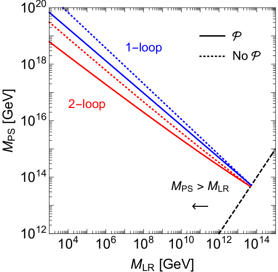
Figure 1: Pati-Salam unification scale as a function of the Left-Right symmetry breaking scale, from a one-loop (blue lines) and a two-loops (red lines) RG analysis. The full (dotted) lines correspond to the case where ${\cal P}$ is broken at the $M_{\rm LR}$ ($M_{\rm PS}$) scale.

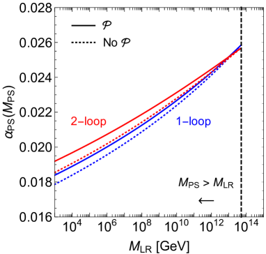
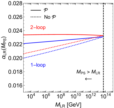
Figure 2: Pati-Salam gauge coupling (left panel) and Left-Right gauge coupling (right panel) at the Pati-Salam unification scale, as a function of the Left-Right symmetry breaking scale.

We can now proceed with the main goal of the RG analysis, namely to express the axion mass as a function of $M_{\rm LR}$, via the relation in Eq. (2.42). This correlation is shown in Fig. 3, where we report directly the two-loop result for the two cases ${\cal G}_{\rm LR}$ (${\cal P}$) and ${\cal G}^{\not{{\cal P}}}_{\rm LR}$ (No ${\cal P}$), together with the current bounds from Black Hole Superradiance and the experimental prospects of future axion DM experiments, whose phenomenological implications are described in the next Section.

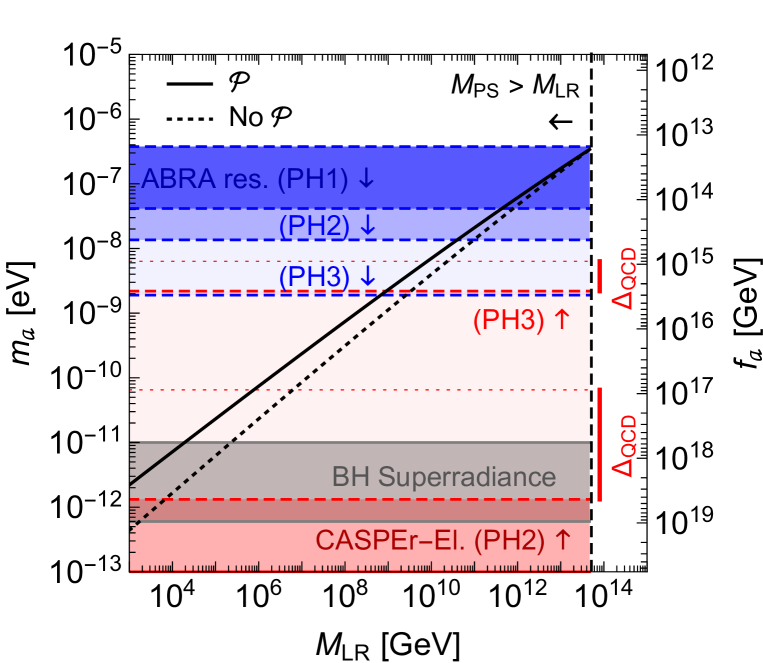
Figure 3: Axion mass dependence from the Left-Right symmetry breaking scale (from two-loop RG analysis). The full (dotted) black line corresponds to the case where ${\cal P}$ is broken at the $M_{\rm LR}$ ($M_{\rm PS}$) scale. The current bound from Black Hole Superradiance (gray) and the future reach in different phases of ABRACADABRA (blue) and CASPEr-Electric (red) are shown as well (see text for details).

3 Phenomenology

From the two-loop RG analysis we have inferred the mass windows displayed in Table 3, where the lower bounds take already into account the exclusion limit in Eq. (3.4). In particular, the correlations among the mass scales can be read off Fig. 1 ($M_{\rm PS}$ vs. $M_{\rm LR}$) and Fig. 3 ($m_{a}$ vs. $M_{\rm LR}$).

	$m_{a}$ [eV]	$M_{\rm LR}$ [GeV]	$M_{\rm PS}$ [GeV]
${\cal G}_{\rm LR}$	$[10^{-11},3.4\times 10^{-7}]$	$[2.0\times 10^{4},4.7\times 10^{13}]$	$[1.4\times 10^{18},4.7\times 10^{13}]$
${\cal G}^{\not{{\cal P}}}_{\rm LR}$	$[10^{-11},3.4\times 10^{-7}]$	$[2.3\times 10^{5},4.7\times 10^{13}]$	$[1.4\times 10^{18},4.7\times 10^{13}]$

Table 3: Mass windows from two-loop RG analysis.

In this Section we discuss the phenomenological implications of those mass ranges, both from the point of view of axion physics and the Pati-Salam/Left-Right symmetry breaking scales.

3.1 Cosmological and astrophysical constraints

Let us start by addressing some relevant cosmological and astrophysical constraints. Very light axion DM tends to be overproduced via the misalignment mechanism [18, 19, 20], and the measured amount of cold DM can only be explained if the PQ symmetry remained broken during inflation and never restored after it, which corresponds to the so-called pre-inflationary PQ breaking scenario (more precisely, the post-inflationary PQ breaking scenario is excluded for $m_{a}\lesssim 30$ $\mu$eV [74]). A late inflationary phase $H_{I}\lesssim M_{\rm PS}\approx f_{a}$ (cf. Eq. (2.40)) is also supported by other cosmological issues of the Pati-Salam axion framework related to the formation of topologically stable defects, which tend to dominate the energy density of the Universe, unless inflated away. These include: $i)$ Magnetic monopoles from Pati-Salam breaking; $ii)$ Domain walls from spontaneous breaking of ${\cal P}$; $iii)$ Axion domain walls at the QCD phase transition. While the domain wall problems are not specific of Pati-Salam and have been widely discussed in the literature (for a review see e.g. [75]), we dwell a bit on the less known physics of Pati-Salam monopoles in Sect. 3.1.1. After that we discuss other constraints related to axion DM (Sect. 3.1.1) and Black Hole Superradiance (Sect. 3.1.3).

3.1.1 Pati-Salam monopoles

Pati-Salam monopoles are topologically stable scalar-gauge field configuration arising from ${\cal G}_{\rm PS}\to{\cal G}_{\rm SM}$ breaking, with magnetic charge $Q_{\rm mag}=4\pi/e$ and mass ${\cal M}_{\rm PS}\sim M_{\rm PS}/\alpha_{\rm PS}$. Although they were originally investigated in the context of intermediate symmetry breaking stages of SO(10) [76, 77, 78], they have some distinct features with respect to GUT monopoles which make them interesting by their own.

A flux of Pati-Salam monopoles hitting an Earth-based detector could actually lead to a spectacular signature, since according to Sen [79, 80] they are expected to catalyze $\Delta(B+L)=3$ violating processes via the weak ‘t Hooft anomaly with a geometrical cross section, i.e. not suppressed by the Pati-Salam breaking scale or by other non-perturbative factors. The conservative Kibble estimate [81] of one monopole per Hubble horizon provides a lower bound on today’s monopole number density (normalized to entropy density)

$$\frac{n_{\rm PS}}{s}\gtrsim\left(\frac{T_{\rm PS}}{M_{\rm Pl}}\right)^{3}\,,$$ (3.1)

where $T_{\rm PS}\approx M_{\rm PS}\gtrsim 10^{13}$ GeV is the critical temperature of the Pati-Salam phase transition. Hence, for the lowest value allowed by the RG analysis, $M_{\rm PS}=4.7\times 10^{13}$ GeV (cf. Table 3) one has $n_{\rm PS}/s\gtrsim 5.7\times 10^{-17}$, which overshoots the critical energy density of the Universe and is also well above the indirect Parker’s bound [85, 86], $n_{\rm PS}/s\lesssim 10^{-26}$, and the direct detection limits from the MACRO Collaboration [87], $n_{\rm PS}/s\lesssim 2\times 10^{-28}$. On the other hand, differently from GUT monopoles, Pati-Salam monopoles are not subject to the much more stringent bounds [88] from the catalysis of proton decay due to the Callan-Rubakov effect [89, 90].

Although in the model considered in this paper Pati-Salam monopoles need to be inflated away, we note that the observational window of two orders of magnitude between the Parker’s bound and direct detection limits might be populated in models with $M_{\rm PS}\ll 10^{13}$ GeV, e.g. in the ballpark of $M_{\rm PS}\approx 10^{10}$ GeV according to the naive Kibble estimate.

3.1.2 Axion relic density and iso-curvature bounds

In the pre-inflationary PQ breaking scenario, the axion’s relic abundance depends both on the mass and on the initial value of the axion field $a_{i}$ in units of the decay constant, $\theta_{i}=a_{i}/f_{a}$, inside the causally connected region which is inflated into our visible Universe, cf. [74, 91]:

$$\Omega_{a}h^{2}=0.12\,\left({3.4\times 10^{-7}~{}{\rm eV}\over m_{a}}\right)^{1.165}\,\left(\frac{\theta_{i}}{0.13}\right)^{2}\,,$$ (3.2)

where we have normalized the axion mass to the upper bound in Table 3 coming from the RG analysis. Thus an axion close to that boundary can reproduce the whole DM, without the need of tuning the initial misalignment angle. In this cosmological scenario, however, iso-curvature quantum fluctuations of a massless axion field during inflation may leave an imprint in the temperature fluctuations of the cosmic microwave background [92, 93], whose amplitude is stringently constrained by observations. In the case that the $\mathcal{S}$ field hosting the axion stays at the broken minimum of the potential throughout inflation (i.e. for the inflaton field not residing in $\mathcal{S}$), those constraints translate into an upper bound on the Hubble expansion rate during inflation [94, 95, 96]

$$H_{I}<9.8\times 10^{7}\,{\rm GeV}\left(\frac{3.4\times 10^{-7}\,\text{eV}}{m_{a}}\right)^{0.4175}\,,$$ (3.3)

which is consistent with a late inflationary phase in order to dilute the cosmic density of monopoles and domain walls.

3.1.3 Black Hole Superradiance

Although super-light axions are free from standard astrophysical bounds due to stellar evolution, they are subject to limits from Black Hole Superradiance as long as the axion decay constant approaches the Planck mass. In fact, axions can form gravitational bound states around black holes whenever their Compton wavelength is of the order of the black holes radii. The phenomenon of superradiance [97] then guarantees that the axion occupation numbers grow exponentially, providing a way to extract very efficiently energy and angular momentum from the black hole [98, 99]. The rate at which the angular momentum is extracted depends on the black hole mass and so the presence of axions could be inferred by observations of black hole masses and spins. A recent analysis excludes the mass window [100]

$$m_{a}\in[6\times 10^{-13},10^{-11}]\ \text{eV}\,,$$ (3.4)

which is shown as a gray band in Fig. 3. It should be stressed that the Black Hole Superradiance bound does not assume the axion being DM and it just relies on the universal axion coupling to gravity through its mass.

3.2 Axion Dark Matter experiments

Axion DM experiments turn out to be the most powerful probes of the Pati-Salam axion (under the assumption that the axion comprises the whole DM), since they can cover the whole mass window $m_{a}\in[10^{-11},3.4\times 10^{-7}]$ eV predicted by the RG analysis (cf. Table 3). In particular, this is possible due to the complementarity of ABRACADABRA [47] and CASPEr-Electric [45, 46], which probe the axion mass parameter space region from opposite directions (cf. Fig. 3).

3.2.1 ABRACADABRA

The axion DM experiment ABRACADABRA [47] has very good prospects to probe the axion-photon coupling for masses $m_{a}\lesssim 4\times 10^{-7}$ eV. Such low values are notoriously difficult to be reached for standard cavity experiments due to the need of matching axion wavelengths with extremely large cavity sizes $\gtrsim 50$ m. ABRACADABRA uses instead a different detection concept based on a toroidal magnet and a pickup loop to detect the variable magnetic flux induced by the oscillating current produced by DM axions in the static (lab) magnetic field. The experiment can operate either in broadband or resonant modus by using an untuned or a tuned magnetometer respectively. A small scale prototype ABRACADABRA-10 cm [101] has already given exclusion limits competitive with astrophysics for axion masses $\in[3.1\times 10^{-10},8.3\times 10^{-9}]$ eV. The projected sensitivities (from [47]) on the axion mass are displayed in Fig. 3 via blue bands. They refer to three different phases of the experiment in the resonant approach, which is more sensitive to the standard QCD axion region, and they also assume $E/N=8/3$, which applies to the Pati-Salam axion considered in this work (cf. Eq. (2.30)) and in general to any GUT axion model.

3.2.2 CASPEr

CASPEr-Electric [45, 46] employs nuclear magnetic resonance techniques to search for an oscillating nEDM [102]

$$d_{n}(t)=g_{d}\,\frac{\sqrt{2\rho_{\text{DM}}}}{m_{a}}\cos(m_{a}\,t)\,,$$ (3.5)

where $g_{d}=C_{an\gamma}/(m_{n}f_{a})$ is the model-independent coupling of the axion to the nEDM operator defined in Eq. (2.23) and $\rho_{\rm DM}\approx 0.4\ \text{GeV}/\text{cm}^{3}$ is the local energy density of axion DM. The numerical value of $C_{an\gamma}$ (cf. Eq. (2.29)) takes over the static nEDM calculation of [103] based on QCD sum rules and amounts to a theoretical error of about $40\%$. In Fig. 3 we show in red bands the axion mass reach of CASPEr-Electric [46] for phases 2 and 3, including as well on the right side of the plot the size of the QCD error (denoted by $\Delta_{\rm QCD}$). Remarkably, the QCD error turns out to be strongly correlated with the projected sensitivities shown in Ref. [46], so that a future reduction of the theoretical error on the static nEDM (e.g. via Lattice QCD techniques [104, 105]) might have a non-trivial impact on the sensitivity reach of CASPEr-Electric.

On the other hand, the projected sensitivity of CASPEr-Wind [46], which exploits the axion nucleon ($N=p,n$) coupling $g_{aN}=C_{aN}/(2f_{a})$ (with $C_{aN}$ given in Eqs. (2.25)–(2.26)) to search for an axion DM wind due to the movement of the Earth through the Galactic DM halo [102], misses the preferred coupling vs. mass region by at least two orders of magnitude, even in its phase 2.

3.3 Pati-Salam signatures

Given the lower bound on the Pati-Salam breaking scale inferred from the RG analysis, $M_{\rm PS}\gtrsim 10^{13}$, genuine signatures of Pati-Salam dynamics turn out to be difficult to be experimentally accessible, as briefly reviewed in the following.

3.3.1 Rare meson decays

The vector leptoquark $\mathcal{X}_{\mu}$ mediates tree-level rare meson decays $K_{L},\,B^{0},B_{s}^{0}\to\ell_{i}\,\ell_{j}$ (for $\ell=(e,\mu,\tau)$), which turn out to be loop- and chirally-enhanced with respect to the SM contribution, and hence provide a powerful flavour probe of the Pati-Salam model [106, 107]. A recent collection of bounds which takes also into account flavour mixing can be found in Ref. [108]. For instance, for maximal mixing the most sensitive channel is $K_{L}\to\mu e$, which probes leptoquark masses up to $10^{6}$ GeV, hence still much below the Pati-Salam breaking scale emerging from the RG analysis.

3.3.2 Baryon number violation

A standard signature of Pati-Salam dynamics are $\Delta B=2$ processes, in particular $n$-$\overline{n}$ oscillations [109], which are described by $d=9$ SM operators of the type

$$\frac{1}{\Lambda^{5}_{\Delta B=2}}\,\left[u_{R}d_{R}d_{R}u_{R}d_{R}d_{R}+q_{L}q_{L}q_{L}q_{L}d_{R}d_{R}\right]\,.$$ (3.6)

Present bounds on nuclear instability and direct reactor oscillations experiments yield bounds at the level of $\Lambda_{\Delta B=2}\gtrsim 100$ TeV [110]. In the present Pati-Salam$\times{\rm U}(1)_{\rm PQ}$ model (see also [36]) only operators of the type $q_{L}q_{L}q_{L}q_{L}d_{R}d_{R}$ are generated, which are mediated by color sextet scalar di-quark fields $\Delta_{qq}$ contained in the Pati-Salam representations $\Delta_{R}\sim(10,1,3)$ and $\Delta_{L}\sim(10,3,1)$, with strength (schematically)

$$\frac{1}{\Lambda^{5}_{\Delta B=2}}\sim\frac{\eta\,y\,v_{R}}{m^{6}_{\Delta_{qq}}}\,,$$ (3.7)

where $\eta$ and $y$ denote respectively the scalar coupling of $\Delta_{R}^{2}\Delta_{L}^{2}$ (cf. Eq. (2.1)) and the Yukawa coupling of $\Delta_{qq}$ to quarks (cf. Eq. (2.1)). Hence, $n$-$\overline{n}$ oscillations could be visible only if those color sextets were unnaturally light $m_{\Delta_{qq}}\ll M_{\rm PS}$.

Nucleon decay from the scalar sector of Pati-Salam is possible as well, as originally observed in [62, 111]. In the presence of the Higgs multiplet $\Phi_{15}\sim(15,2,2)$, required by a realistic fit to SM fermion masses, the spontaneous breaking of ${\rm U}(1)_{B-L}$ can lead to $B+L$ preserving nucleon decay modes of the type $N\to\ell+\text{meson}$ or even three-lepton decay modes $N\to\ell+\overline{\ell}+\ell$ [112], associated respectively to $d=9$ and $d=10$ SM effective operators, whose short-distance origin can be traced back into the scalar potential couplings $\gamma_{15}$ and $\delta_{15}$ in Eq. (2.1) (see [36] for a more detailed account). As in the case of $n$-$\overline{n}$ oscillations, for these exotic nucleon decay modes to be observable, one or more scalar fragments of $\Phi_{15}$ and $\Delta_{R,L}$ mediating those nucleon decay operators need to be $\lesssim 100$ TeV, unnaturally light compared to the Pati-Salam breaking scale.

3.4 Left-Right signatures

A sliding Left-Right symmetry breaking scale $M_{\rm LR}\in[2.0\times 10^{4},4.7\times 10^{13}]$ GeV (e.g. in the case of ${\cal P}$ broken at the $M_{\rm LR}$ scale, cf. Table 3) offers potentially observables signatures related to the Left-Right breaking dynamics, together with the possibility of observing a correlated signal with axion physics. In the following, we consider two opposite scenarios in which the Left-Right symmetry is broken either at high or low scales.

3.4.1 High-scale Left-Right breaking

The high-scale Left-Right breaking scenario, corresponding to a single step breaking with $M_{\rm LR}\approx M_{\rm PS}\approx 4.7\times 10^{13}$ GeV is motivated by naturalness arguments. In fact, it simultaneously minimizes the parameter space tuning in three sectors of the theory: $i)$ it avoids the extra $(M_{\rm LR}/M_{\rm PS})^{2}$ tuning of triplet fields (cf. Table 2); $ii)$ it reduces the tuning of the initial axion misalignment angle in order not to overshoot the axion DM relic density (cf. Eq. (3.2)); $iii)$ it mitigates the tuning in the Dirac neutrino mass matrix, which turns out to be strongly correlated with the up-quark mass matrix (cf. Eq. (2.8) and (2.11)), and hence it prefers high values of $M_{\rm LR}$ in order not to overshoot light neutrino masses (cf. Eq. (2.15)). Moreover, we note that the single-step breaking corresponds to the lower end of the axion mass window $m_{a}\approx 3\times 10^{-7}$ GeV, which will be one of the first region to be tested, already in Phase 1 of ABRACADABRA (cf. Fig. 3).

In fact, a detailed fit of SM fermion masses and mixings within the minimal renormalizable Yukawa sector (cf. the mass sum rules in Eqs. (2.8)–(2.10) and Eq. (2.15)) could actually reveal a non-trivial constraint on the model and select an intermediate-scale value for $M_{\rm LR}\gg$ TeV. An independent argument for high-scale Left-Right breaking is given by thermal leptogenesis [11], which in its simplest realization would suggest $M_{\rm LR}\gtrsim 10^{9}$ GeV (see e.g. [12]).

Finally, in the presence of a strong first-order phase transition the Left-Right symmetry breaking can lead to the production of a stochastic gravitational wave background, that might leave its imprint on the gravitational wave spectrum of forthcoming space-based interferometers [115]. This can happen in some parameter space regions of the Left-Right symmetric scalar potential, resembling an approximate scale invariance [116]. The latter work focussed on Left-Right breaking scales close to the TeV scale, but in principle detectable gravitational wave signals might arise also for $M_{\rm LR}\gg$ TeV.

3.4.2 Low-scale Left-Right breaking

The Left-Right symmetry breaking scale can be as low as 20 TeV (230 TeV) in the case where ${\cal P}$ is broken at the $M_{\rm LR}$ ($M_{\rm PS}$) scale (cf. Table 3). In particular, the lower bound is saturated in both cases for $M_{\rm PS}=1.4\times 10^{18}$ GeV, or equivalently (cf. Eq. (2.40)) for a Pati-Salam/Peccei-Quinn breaking order parameter $v_{\mathcal{S}}=3.4\times 10^{18}$ GeV, that is of the order of the reduced Planck mass $M_{\rm Pl}/\sqrt{8\pi}$. Although this numerical coincidence should not be taken too seriously, since it might be spoiled by scalar threshold effects, it is suggestive of a possible connection with gravity and it could be seen as a mild theoretical motivation for a low-scale Left-Right symmetry breaking scenario. In particular, the former case of ${\cal P}$ broken at $M_{\rm LR}$, corresponds to the most constrained version of the Left-Right symmetric model [3, 4], whose phenomenology has beed studied in great detail in the recent years (see e.g. [117, 118, 119]). Although a $W_{R}$ mass of the order of 20 TeV is well beyond the direct/indirect $\approx 6$ TeV reach of the LHC [120, 121, 122, 123], flavour [119] and CP [59, 60] violating observables offer sensitivities up to hundreds of TeV. A future 100 TeV hadron collider would be able instead to directly probe the lower end of the $M_{\rm LR}$ range, possibly in correlation with an axion signal at CASPEr-Electric for $m_{a}\gtrsim 10^{-11}$ eV.

4 Conclusions

In this work we have discussed the implementation of the PQ mechanism in a minimal realization of the Pati-Salam (partial) unification scheme, where the axion mass is related to the Pati-Salam breaking scale. The latter was shown to be constrained by a RG analysis of (partial) gauge coupling unification. The main physics result is displayed in Fig. 3, which shows that the whole parameter space of the Pati-Salam axion will be probed in the late phases of the axion DM experiments ABRACADABRA and CASPEr-Electric. Possible correlated signatures connected with the breaking of the Left-Right symmetry group include future collider/flavour probes of a low-scale Left-Right breaking (as low as 20 TeV for a Pati-Salam breaking of the size of the reduced Planck mass – cf. Fig. 1) and, less generically, the imprint on the gravitational wave spectrum of the Left-Right phase transition. Other indirect constraints on the scale of Left-Right symmetry breaking might arise from a detailed fit of SM fermion masses and mixings within the minimal renormalizable Pati-Salam Yukawa sector or from a successful implementation of thermal leptogenesis. Both of them could be worth a future investigation, in order to further narrow down an axion mass range. Finally, some of the ingredients discussed in the present paper might serve as building blocks for a detailed investigation of what could arguably be considered the minimal ${\rm SO}(10)\times{\rm U}(1)_{\rm PQ}$ model, based on a $45_{H}+\overline{126}_{H}+10_{H}$ reducible Higgs representation [124, 125], with a complex adjoint hosting the SO(10) axion.

While in the Introduction we have praised the nice aspects of the whole setup, here we would like to conclude with a more critical note. In the present formulation (as well as in all GUT$\times{\rm U}(1)_{\rm PQ}$ models known to the author and despite some earlier attempts of obtaining an automatic ${\rm U}(1)_{\rm PQ}$ from SU(9) [126]) the PQ symmetry is imposed by hand, while it would be more satisfactory for it to arise as an accidental symmetry, possibly due to some underlying gauge dynamics. Moreover, since global symmetries need not to be exact, it is unclear why the PQ symmetry should be an extremely good symmetry of UV physics, and in particular of quantum gravity, not to spoil the solution of the strong CP problem [127, 128, 129]. This is particularly problematic for axion GUTs, since the issue gets worse in the $f_{a}\to M_{\rm Pl}$ limit. While we have nothing to say on this important problem, it would be desirable to have some fresh new ideas on how to tackle it (especially in GUTs). For the time being, we can pragmatically postpone the question until the discovery of the axion.

Appendix A Two-loop running and one-loop matching

In this Appendix we collect the two-loop beta functions and the one-loop matching coefficient employed in the RG analysis.

Two-loop beta functions

Let us denote the product of gauge factors $G=G_{1}\times\ldots\times G_{N}$. The two-loop RG equations for the corresponding gauge couplings $g_{i}$ ($i=1,\ldots,N$) can be written as

$$\mu\frac{d}{d\mu}\alpha^{-1}_{i}=-\frac{a_{i}}{2\pi}-\sum_{j}\frac{b_{ij}}{8\pi^{2}}\alpha_{j}\,,$$ (A.1)

where $\alpha_{i}=g_{i}^{2}/(4\pi)$. The one- and two-loop beta coefficients in the $\overline{\rm MS}$ scheme are [130] (no summation over $i$)

$$a_{i} =-\frac{11}{3}C_{2}(G_{i})+\frac{4}{3}\sum_{F}\kappa S_{2}(F_{i})+\frac{1}{3}\sum_{S}\eta S_{2}(S_{i})\,,$$ (A.2)

$$b_{ij} =\left[-\frac{34}{3}\left(C_{2}(G_{i})\right)^{2}+\sum_{F}\left(4C_{2}(F_{i})+\frac{20}{3}C_{2}(G_{i})\right)\kappa S_{2}(F_{i})\right.$$

$$\left.+\sum_{S}\left(4C_{2}(S_{i})+\frac{2}{3}C_{2}(G_{i})\right)\eta S_{2}(S_{i})\right]\delta_{ij}$$

$$+4\Big{[}\sum_{F}\kappa C_{2}(F_{j})S_{2}(F_{i})+\sum_{S}\eta C_{2}(S_{j})S_{2}(S_{i})\Big{]}\,,$$ (A.3)

where $G_{i}$ denotes the $i$-th gauge factor, $S_{2}(R_{i})=T(R_{i})d(R)/d(R_{i})$ in terms of the Dynkin index (with normalization $\frac{1}{2}$ for the fundamental) of the representation $R_{i}$, $T(R_{i})$, and the multiplicity factor $d(R)/d(R_{i})$, with $d(R_{i})$ ($d(R)$) denoting the dimension of the representation under $G_{i}$ ($G$). The latter are related to the Casimir invariant, $C_{2}(R_{i})$, via $C_{2}(R_{i})d(R_{i})=T(R_{i})d(G_{i})$, where $d(G_{i})$ is the dimension of $G_{i}$. $\kappa=1,\frac{1}{2}$ for Dirac, Weyl fermions ($F$) and $\eta=1,\frac{1}{2}$ for complex, real scalar ($S$) fields, respectively. The Yukawa contribution in the two-loop beta coefficient has been neglected.

Specifically, for the two running stages considered in this work we have (using the ESH intermediate-scale scalars in Table 2):

• ${\cal G}_{\rm SM}\equiv{\rm SU}(3)_{C}\times{\rm SU}(2)_{L}\times{\rm U}(1)_{Y}$ ($M_{Z}\to M_{\rm LR}$ running)

  $$a^{\rm SM}=\left(-7,-\tfrac{19}{6},\tfrac{41}{10}\right)\,,\qquad b^{\rm SM}=\left(\begin{array}[]{ccc}-26&\frac{9}{2}&\frac{11}{10}\\ 12&\frac{35}{6}&\frac{9}{10}\\ \frac{44}{5}&\frac{27}{10}&\frac{199}{50}\\ \end{array}\right)\,.$$ (A.4)

• ${\cal G}_{\rm LR}\equiv{\rm SU}(3)_{C}\times{\rm SU}(2)_{L}\times{\rm SU}(2)_{R}\times{\rm U}(1)_{B-L}\times{\cal P}$ ($M_{\rm LR}\to M_{\rm PS}$ running)

  $$a^{\rm LR}=\left(-7,-\tfrac{7}{3},-\tfrac{7}{3},7\right)\,,\qquad b^{\rm LR}=\left(\begin{array}[]{cccc}-26&\frac{9}{2}&\frac{9}{2}&\frac{11}{2}\\ 12&\frac{80}{3}&3&\frac{297}{2}\\ 12&3&\frac{80}{3}&\frac{297}{2}\\ 4&\frac{81}{2}&\frac{81}{2}&\frac{1265}{2}\\ \end{array}\right)\,.$$ (A.5)

• ${\cal G}^{\not{{\cal P}}}_{\rm LR}\equiv{\rm SU}(3)_{C}\times{\rm SU}(2)_{L}\times{\rm SU}(2)_{R}\times{\rm U}(1)_{B-L}$ ($M_{\rm LR}\to M_{\rm PS}$ running)

  $$a^{\rm LR}=\left(-7,-3,-\tfrac{7}{3},\tfrac{11}{2}\right)\,,\qquad b^{\rm LR}=\left(\begin{array}[]{cccc}-26&\frac{9}{2}&\frac{9}{2}&\frac{11}{2}\\ 12&8&3&\frac{33}{2}\\ 12&3&\frac{80}{3}&\frac{297}{2}\\ 4&\frac{9}{2}&\frac{81}{2}&\frac{671}{2}\\ \end{array}\right)\,.$$ (A.6)

  where we considered both the case in which ${\cal P}$ is broken at the $M_{\rm LR}$ scale (${\cal G}_{\rm LR}$) and at the $M_{\rm PS}$ scale (${\cal G}^{\not{{\cal P}}}_{\rm LR}$)

One-loop matching coefficients

The general form of the one-loop matching condition between effective theories in the framework of dimensional regularization was derived in [131, 132] (see also [10] for the inclusion of ${\rm U}(1)$ mixing). Considering for definiteness the case of a simple group $G$ spontaneously broken into subgroups $G_{i}$, the one-loop matching (at the matching scale $\mu$) for the gauge couplings can be written as [133]

$$\alpha^{-1}_{i}(\mu)=\alpha^{-1}(\mu)-4\pi\lambda^{i}(\mu)\,,$$ (A.7)

where

$$\lambda^{i}(\mu) =\frac{1}{12\pi}(C_{2}(G)-C_{2}(G_{i}))$$

$$+\frac{1}{2\pi}\left[-\frac{11}{3}\mbox{Tr}\,T_{V_{i}}^{2}\log\frac{M_{V_{i}}}{\mu}+\frac{4}{3}\kappa\mbox{Tr}\,T_{F_{i}}^{2}\log\frac{M_{F_{i}}}{\mu}+\frac{1}{3}\eta\mbox{Tr}\,T_{S_{i}}^{2}\log\frac{M_{S_{i}}}{\mu}\right]\,,$$ (A.8)

with $V$, $F$ and $S$ denoting the massive vectors, fermions and scalars that are integrated out at the matching scale $\mu$. Note that differently from [131, 132] the (Feynman gauge) Goldstone bosons have been conveniently included in the scalar part of the expression, so that the matching coefficients resembles the structure of the one-loop beta coefficients in Eq. (A.2).

Specifically, for the two matching scales considered in this work we have:

• $M_{\rm LR}$ (${\cal G}_{\rm SM}\leftrightarrow{\cal G}^{(\not{{\cal P}})}_{\rm LR}$ matching)

  $$\alpha_{1}^{-1}(M_{\rm LR}) =\frac{3}{5}\left(\alpha_{R}^{-1}(M_{\rm LR})-\frac{1}{6\pi}\right)+\frac{2}{5}\alpha_{B-L}^{-1}(M_{\rm LR})\,,$$ (A.9)

  $$\alpha_{L}(M_{\rm LR}) =\alpha_{L}(M_{\rm LR})\,,$$ (A.10)

  $$\alpha_{C}(M_{\rm LR}) =\alpha_{C}(M_{\rm LR})\,.$$ (A.11)

• $M_{\rm PS}$ (${\cal G}^{(\not{{\cal P}})}_{\rm LR}\leftrightarrow{\cal G}_{\rm PS}$ matching)

  $$\alpha^{-1}_{B-L}(M_{\rm PS}) =\alpha_{C}^{-1}(M_{\rm PS})-\frac{1}{4\pi}=\alpha_{\rm PS}^{-1}(M_{\rm PS})-\frac{1}{3\pi}\,,$$ (A.12)

  $$\alpha_{R}(M_{\rm PS}) =\alpha_{L}(M_{\rm PS})=\alpha_{\rm LR}(M_{\rm PS})\,.$$ (A.13)

References

- [1] J. C. Pati and A. Salam, “Lepton Number as the Fourth Color,” Phys. Rev. D 10 (1974) 275–289. [Erratum: Phys.Rev.D 11, 703–703 (1975)].
- [2] R. N. Mohapatra and J. C. Pati, “A Natural Left-Right Symmetry,” Phys. Rev. D11 (1975) 2558.
- [3] G. Senjanovic and R. N. Mohapatra, “Exact Left-Right Symmetry and Spontaneous Violation of Parity,” Phys. Rev. D 12 (1975) 1502.
- [4] R. N. Mohapatra and G. Senjanovic, “Neutrino Mass and Spontaneous Parity Nonconservation,” Phys. Rev. Lett. 44 (1980) 912.
- [5] H. Fritzsch and P. Minkowski, “Unified Interactions of Leptons and Hadrons,” Annals Phys. 93 (1975) 193–266.
- [6] H. Georgi, “The State of the Art-Gauge Theories,” AIP Conf. Proc. 23 (1975) 575–582.
- [7] A. Melfo and G. Senjanovic, “Minimal supersymmetric Pati-Salam theory: Determination of physical scales,” Phys. Rev. D 68 (2003) 035013, arXiv:hep-ph/0302216.
- [8] D. Chang, R. Mohapatra, J. Gipson, R. Marshak, and M. Parida, “Experimental Tests of New SO(10) Grand Unification,” Phys. Rev. D 31 (1985) 1718.
- [9] N. G. Deshpande, E. Keith, and P. B. Pal, “Implications of LEP results for SO(10) grand unification with two intermediate stages,” Phys. Rev. D47 (1993) 2892–2896, arXiv:hep-ph/9211232 [hep-ph].
- [10] S. Bertolini, L. Di Luzio, and M. Malinsky, “Intermediate mass scales in the non-supersymmetric SO(10) grand unification: A Reappraisal,” Phys. Rev. D 80 (2009) 015013, arXiv:0903.4049 [hep-ph].
- [11] M. Fukugita and T. Yanagida, “Baryogenesis Without Grand Unification,” Phys. Lett. B 174 (1986) 45–47.
- [12] S. Davidson, E. Nardi, and Y. Nir, “Leptogenesis,” Phys. Rept. 466 (2008) 105–177, arXiv:0802.2962 [hep-ph].
- [13] M. Nemevsek, G. Senjanovic, and Y. Zhang, “Warm Dark Matter in Low Scale Left-Right Theory,” JCAP 07 (2012) 006, arXiv:1205.0844 [hep-ph].
- [14] R. Peccei and H. R. Quinn, “CP Conservation in the Presence of Instantons,” Phys. Rev. Lett. 38 (1977) 1440–1443.
- [15] R. Peccei and H. R. Quinn, “Constraints Imposed by CP Conservation in the Presence of Instantons,” Phys. Rev. D 16 (1977) 1791–1797.
- [16] S. Weinberg, “A New Light Boson?,” Phys. Rev. Lett. 40 (1978) 223–226.
- [17] F. Wilczek, “Problem of Strong and Invariance in the Presence of Instantons,” Phys. Rev. Lett. 40 (1978) 279–282.
- [18] J. Preskill, M. B. Wise, and F. Wilczek, “Cosmology of the Invisible Axion,” Phys. Lett. B 120 (1983) 127–132.
- [19] L. Abbott and P. Sikivie, “A Cosmological Bound on the Invisible Axion,” Phys. Lett. B 120 (1983) 133–136.
- [20] M. Dine and W. Fischler, “The Not So Harmless Axion,” Phys. Lett. B 120 (1983) 137–141.
- [21] K. Babu and R. Mohapatra, “Predictive neutrino spectrum in minimal SO(10) grand unification,” Phys. Rev. Lett. 70 (1993) 2845–2848, arXiv:hep-ph/9209215.
- [22] L. Di Luzio, M. Giannotti, E. Nardi, and L. Visinelli, “The landscape of QCD axion models,” arXiv:2003.01100 [hep-ph].
- [23] R. N. Mohapatra and G. Senjanovic, “The Superlight Axion and Neutrino Masses,” Z. Phys. C 17 (1983) 53–56.
- [24] A. Davidson and K. C. Wali, “Minimal flavour unification via multigenerational Peccei-Quinn symmetry,” Phys. Rev. Lett. 48 (1982) 11.
- [25] D. B. Reiss, “Invisible axion at an intermediate symmetry breaking scale,” Phys. Lett. 109B (1982) 365–368.
- [26] G. Lazarides, “SO(10) and the Invisible Axion,” Phys. Rev. D 25 (1982) 2425.
- [27] R. Holman, G. Lazarides, and Q. Shafi, “Axions and the Dark Matter of the Universe,” Phys. Rev. D 27 (1983) 995.
- [28] S. Kalara and R. N. Mohapatra, “Geometric Gauge Hierarchy in a Supersymmetric SO(10) X U(1) Pq Model,” Phys. Rev. D28 (1983) 2241.
- [29] A. Davidson, V. P. Nair, and K. C. Wali, “Peccei-Quinn Symmetry as Flavor Symmetry and Grand Unification,” Phys. Rev. D29 (1984) 1504.
- [30] A. Davidson, V. P. Nair, and K. C. Wali, “Mixing Angles and CP Violation in the SO(10) X U(1)-(pq) Model,” Phys. Rev. D29 (1984) 1513.
- [31] D. Chang and G. Senjanovic, “On Axion and Familons,” Phys. Lett. B188 (1987) 231.
- [32] T. Fukuyama and T. Kikuchi, “Axion and right-handed neutrino in the minimal SUSY SO(10) model,” JHEP 05 (2005) 017, arXiv:hep-ph/0412373 [hep-ph].
- [33] B. Bajc, A. Melfo, G. Senjanovic, and F. Vissani, “Yukawa sector in non-supersymmetric renormalizable SO(10),” Phys. Rev. D 73 (2006) 055001, arXiv:hep-ph/0510139.
- [34] G. Altarelli and D. Meloni, “A non supersymmetric SO(10) grand unified model for all the physics below ,” JHEP 08 (2013) 021, arXiv:1305.1001 [hep-ph].
- [35] K. Babu and S. Khan, “Minimal nonsupersymmetric model: Gauge coupling unification, proton decay, and fermion masses,” Phys. Rev. D 92 no. 7, (2015) 075018, arXiv:1507.06712 [hep-ph].
- [36] S. Saad, “Fermion Masses and Mixings, Leptogenesis and Baryon Number Violation in Pati-Salam Model,” Nucl. Phys. B 943 (2019) 114630, arXiv:1712.04880 [hep-ph].
- [37] A. Ernst, A. Ringwald, and C. Tamarit, “Axion Predictions in Models,” JHEP 02 (2018) 103, arXiv:1801.04906 [hep-ph].
- [38] A. Ernst, L. Di Luzio, A. Ringwald, and C. Tamarit, “Axion properties in GUTs,” PoS CORFU2018 (2019) 054, arXiv:1811.11860 [hep-ph].
- [39] S. M. Boucenna, T. Ohlsson, and M. Pernow, “A minimal non-supersymmetric SO(10) model with Peccei–Quinn symmetry,” Phys. Lett. B792 (2019) 251–257, arXiv:1812.10548 [hep-ph]. [Erratum: Phys. Lett.B797,134902(2019)].
- [40] K. S. Babu, T. Fukuyama, S. Khan, and S. Saad, “Peccei-Quinn Symmetry and Nucleon Decay in Renormalizable SUSY (10),” JHEP 06 (2019) 045, arXiv:1812.11695 [hep-ph].
- [41] Y. Hamada, M. Ibe, Y. Muramatsu, K.-y. Oda, and N. Yokozaki, “Proton Decay and Axion Dark Matter in SO(10) Grand Unification via Minimal Left-Right Symmetry,” arXiv:2001.05235 [hep-ph].
- [42] G. Lazarides and Q. Shafi, “Axion Model with Intermediate Scale Fermionic Dark Matter,” arXiv:2004.11560 [hep-ph].
- [43] P. Sikivie, “Invisible Axion Search Methods,” arXiv:2003.02206 [hep-ph].
- [44] I. G. Irastorza and J. Redondo, “New experimental approaches in the search for axion-like particles,” Prog. Part. Nucl. Phys. 102 (2018) 89–159, arXiv:1801.08127 [hep-ph].
- [45] D. Budker, P. W. Graham, M. Ledbetter, S. Rajendran, and A. Sushkov, “Proposal for a Cosmic Axion Spin Precession Experiment (CASPEr),” Phys. Rev. X4 no. 2, (2014) 021030, arXiv:1306.6089 [hep-ph].
- [46] D. F. Jackson Kimball et al., “Overview of the Cosmic Axion Spin Precession Experiment (CASPEr),” arXiv:1711.08999 [physics.ins-det].
- [47] Y. Kahn, B. R. Safdi, and J. Thaler, “Broadband and Resonant Approaches to Axion Dark Matter Detection,” Phys. Rev. Lett. 117 no. 14, (2016) 141801, arXiv:1602.01086 [hep-ph].
- [48] L. Di Luzio, A. Ringwald, and C. Tamarit, “Axion mass prediction from minimal grand unification,” Phys. Rev. D 98 no. 9, (2018) 095011, arXiv:1807.09769 [hep-ph].
- [49] B. Bajc and G. Senjanovic, “Seesaw at LHC,” JHEP 08 (2007) 014, arXiv:hep-ph/0612029.
- [50] B. Bajc, M. Nemevsek, and G. Senjanovic, “Probing seesaw at LHC,” Phys. Rev. D 76 (2007) 055011, arXiv:hep-ph/0703080.
- [51] L. Di Luzio and L. Mihaila, “Unification scale vs. electroweak-triplet mass in the model at three loops,” Phys. Rev. D 87 (2013) 115025, arXiv:1305.2850 [hep-ph].
- [52] P. Fileviez P rez, C. Murgui, and A. D. Plascencia, “The QCD Axion and Unification,” JHEP 11 (2019) 093, arXiv:1908.01772 [hep-ph].
- [53] P. Fileviez P rez, C. Murgui, and A. D. Plascencia, “Axion Dark Matter, Proton Decay and Unification,” JHEP 01 (2020) 091, arXiv:1911.05738 [hep-ph].
- [54] R. T. Co, F. D’Eramo, and L. J. Hall, “Supersymmetric axion grand unified theories and their predictions,” Phys. Rev. D 94 no. 7, (2016) 075001, arXiv:1603.04439 [hep-ph].
- [55] T. Kibble, G. Lazarides, and Q. Shafi, “Strings in SO(10),” Phys. Lett. B 113 (1982) 237–239.
- [56] T. Kibble, G. Lazarides, and Q. Shafi, “Walls Bounded by Strings,” Phys. Rev. D 26 (1982) 435.
- [57] D. Chang, R. Mohapatra, and M. Parida, “Decoupling Parity and SU(2)-R Breaking Scales: A New Approach to Left-Right Symmetric Models,” Phys. Rev. Lett. 52 (1984) 1072.
- [58] D. Chang, R. Mohapatra, and M. Parida, “A New Approach to Left-Right Symmetry Breaking in Unified Gauge Theories,” Phys. Rev. D 30 (1984) 1052.
- [59] A. Maiezza and M. Nemevsek, “Strong P invariance, neutron electric dipole moment, and minimal left-right parity at LHC,” Phys. Rev. D 90 no. 9, (2014) 095002, arXiv:1407.3678 [hep-ph].
- [60] S. Bertolini, A. Maiezza, and F. Nesti, “Kaon CP violation and neutron EDM in the minimal left-right symmetric model,” Phys. Rev. D 101 no. 3, (2020) 035036, arXiv:1911.09472 [hep-ph].
- [61] G. Senjanovic and V. Tello, “Strong CP violation: problem or blessing?,” arXiv:2004.04036 [hep-ph].
- [62] J. C. Pati, A. Salam, and U. Sarkar, “Delta B = - Delta L, neutron e- pi+, e- K+, mu- pi+ and mu- K+ DECAY modes in SU(2)-L x SU(2)-R x SU(4)-C or SO(10),” Phys. Lett. 133B (1983) 330–336.
- [63] A. S. Joshipura and K. M. Patel, “Fermion Masses in SO(10) Models,” Phys. Rev. D 83 (2011) 095002, arXiv:1102.5148 [hep-ph].
- [64] S. Bertolini, L. Di Luzio, and F. Nesti, “Axion properties in Left-Right symmetric models,” (2020, In preparation) .
- [65] M. Srednicki, “Axion Couplings to Matter. 1. CP Conserving Parts,” Nucl. Phys. B 260 (1985) 689–700.
- [66] G. Grilli di Cortona, E. Hardy, J. Pardo Vega, and G. Villadoro, “The QCD axion, precisely,” JHEP 01 (2016) 034, arXiv:1511.02867 [hep-ph].
- [67] M. Pospelov and A. Ritz, “Theta induced electric dipole moment of the neutron via QCD sum rules,” Phys. Rev. Lett. 83 (1999) 2526–2529, arXiv:hep-ph/9904483.
- [68] D. Buttazzo, L. Di Luzio, P. Ghorbani, C. Gross, G. Landini, A. Strumia, D. Teresi, and J.-W. Wang, “Scalar gauge dynamics and Dark Matter,” JHEP 01 (2020) 130, arXiv:1911.04502 [hep-ph].
- [69] L. Di Luzio, J. Fuentes-Martin, A. Greljo, M. Nardecchia, and S. Renner, “Maximal Flavour Violation: a Cabibbo mechanism for leptoquarks,” JHEP 11 (2018) 081, arXiv:1808.00942 [hep-ph].
- [70] M. Gorghetto and G. Villadoro, “Topological Susceptibility and QCD Axion Mass: QED and NNLO corrections,” JHEP 03 (2019) 033, arXiv:1812.01008 [hep-ph].
- [71] F. del Aguila and L. E. Ibanez, “Higgs Bosons in SO(10) and Partial Unification,” Nucl. Phys. B 177 (1981) 60–86.
- [72] R. N. Mohapatra and G. Senjanovic, “Higgs Boson Effects in Grand Unified Theories,” Phys. Rev. D 27 (1983) 1601.
- [73] L. N. Mihaila, J. Salomon, and M. Steinhauser, “Renormalization constants and beta functions for the gauge couplings of the Standard Model to three-loop order,” Phys. Rev. D 86 (2012) 096008, arXiv:1208.3357 [hep-ph].
- [74] S. Borsanyi et al., “Calculation of the axion mass based on high-temperature lattice quantum chromodynamics,” Nature 539 no. 7627, (2016) 69–71, arXiv:1606.07494 [hep-lat].
- [75] A. Vilenkin, “Cosmic Strings and Domain Walls,” Phys. Rept. 121 (1985) 263–315.
- [76] G. Lazarides and Q. Shafi, “The Fate of Primordial Magnetic Monopoles,” Phys. Lett. 94B (1980) 149–152.
- [77] G. Lazarides, M. Magg, and Q. Shafi, “Phase Transitions and Magnetic Monopoles in SO(10),” Phys. Lett. 97B (1980) 87–92.
- [78] S. Dawson and A. N. Schellekens, “Monopole Catalysis of Proton Decay in SO(10) Grand Unified Models,” Phys. Rev. D27 (1983) 2119.
- [79] A. Sen, “Baryon Number Violation Induced by the Monopoles of the Pati-Salam Model,” Phys. Lett. B 153 (1985) 55–58.
- [80] A. Sen, “Monopole Induced Baryon Number Violation Due to Weak Anomaly,” Nucl. Phys. B250 (1985) 1–38.
- [81] T. W. B. Kibble, “Topology of Cosmic Domains and Strings,” J. Phys. A9 (1976) 1387–1398.
- [82] W. H. Zurek, “Cosmological Experiments in Superfluid Helium?,” Nature 317 (1985) 505–508.
- [83] H. Murayama and J. Shu, “Topological Dark Matter,” Phys. Lett. B 686 (2010) 162–165, arXiv:0905.1720 [hep-ph].
- [84] V. V. Khoze and G. Ro, “Dark matter monopoles, vectors and photons,” JHEP 10 (2014) 061, arXiv:1406.2291 [hep-ph].
- [85] E. N. Parker, “The Origin of Magnetic Fields,” Astrophys. J. 160 (1970) 383.
- [86] M. S. Turner, E. N. Parker, and T. J. Bogdan, “Magnetic Monopoles and the Survival of Galactic Magnetic Fields,” Phys. Rev. D26 (1982) 1296.
- [87] MACRO Collaboration, M. Ambrosio et al., “Final results of magnetic monopole searches with the MACRO experiment,” Eur. Phys. J. C25 (2002) 511–522, arXiv:hep-ex/0207020 [hep-ex].
- [88] Super-Kamiokande Collaboration, K. Ueno et al., “Search for GUT monopoles at Super–Kamiokande,” Astropart. Phys. 36 (2012) 131–136, arXiv:1203.0940 [hep-ex].
- [89] C. G. Callan, Jr., “Dyon-Fermion Dynamics,” Phys. Rev. D26 (1982) 2058–2068.
- [90] V. A. Rubakov, “Adler-Bell-Jackiw Anomaly and Fermion Number Breaking in the Presence of a Magnetic Monopole,” Nucl. Phys. B203 (1982) 311–348.
- [91] G. Ballesteros, J. Redondo, A. Ringwald, and C. Tamarit, “Standard Model-axion-seesaw-Higgs portal inflation. Five problems of particle physics and cosmology solved in one stroke,” JCAP 1708 (2017) 001, arXiv:1610.01639 [hep-ph].
- [92] A. D. Linde, “Generation of Isothermal Density Perturbations in the Inflationary Universe,” Phys. Lett. 158B (1985) 375–380.
- [93] D. Seckel and M. S. Turner, “Isothermal Density Perturbations in an Axion Dominated Inflationary Universe,” Phys. Rev. D32 (1985) 3178.
- [94] M. Beltran, J. Garcia-Bellido, and J. Lesgourgues, “Isocurvature bounds on axions revisited,” Phys. Rev. D75 (2007) 103507, arXiv:hep-ph/0606107 [hep-ph].
- [95] M. P. Hertzberg, M. Tegmark, and F. Wilczek, “Axion Cosmology and the Energy Scale of Inflation,” Phys. Rev. D78 (2008) 083507, arXiv:0807.1726 [astro-ph].
- [96] J. Hamann, S. Hannestad, G. G. Raffelt, and Y. Y. Y. Wong, “Isocurvature forecast in the anthropic axion window,” JCAP 0906 (2009) 022, arXiv:0904.0647 [hep-ph].
- [97] R. Penrose, “Gravitational collapse: The role of general relativity,” Riv. Nuovo Cim. 1 (1969) 252–276. [Gen. Rel. Grav.34,1141(2002)].
- [98] A. Arvanitaki and S. Dubovsky, “Exploring the String Axiverse with Precision Black Hole Physics,” Phys. Rev. D 83 (2011) 044026, arXiv:1004.3558 [hep-th].
- [99] A. Arvanitaki, M. Baryakhtar, and X. Huang, “Discovering the QCD Axion with Black Holes and Gravitational Waves,” Phys. Rev. D 91 no. 8, (2015) 084011, arXiv:1411.2263 [hep-ph].
- [100] V. Cardoso, . J. Dias, G. S. Hartnett, M. Middleton, P. Pani, and J. E. Santos, “Constraining the mass of dark photons and axion-like particles through black-hole superradiance,” JCAP 03 (2018) 043, arXiv:1801.01420 [gr-qc].
- [101] J. L. Ouellet et al., “First Results from ABRACADABRA-10 cm: A Search for Sub-eV Axion Dark Matter,” Phys. Rev. Lett. 122 no. 12, (2019) 121802, arXiv:1810.12257 [hep-ex].
- [102] P. W. Graham and S. Rajendran, “New Observables for Direct Detection of Axion Dark Matter,” Phys. Rev. D88 (2013) 035023, arXiv:1306.6088 [hep-ph].
- [103] M. Pospelov and A. Ritz, “Theta vacua, QCD sum rules, and the neutron electric dipole moment,” Nucl. Phys. B573 (2000) 177–200, arXiv:hep-ph/9908508 [hep-ph].
- [104] M. Abramczyk, S. Aoki, T. Blum, T. Izubuchi, H. Ohki, and S. Syritsyn, “Lattice calculation of electric dipole moments and form factors of the nucleon,” Phys. Rev. D 96 no. 1, (2017) 014501, arXiv:1701.07792 [hep-lat].
- [105] J. Dragos, T. Luu, A. Shindler, J. de Vries, and A. Yousif, “Confirming the Existence of the strong CP Problem in Lattice QCD with the Gradient Flow,” arXiv:1902.03254 [hep-lat].
- [106] G. Valencia and S. Willenbrock, “Quark - lepton unification and rare meson decays,” Phys. Rev. D50 (1994) 6843–6848, arXiv:hep-ph/9409201 [hep-ph].
- [107] A. V. Kuznetsov and N. V. Mikheev, “Vector leptoquarks could be rather light?,” Phys. Lett. B329 (1994) 295–299, arXiv:hep-ph/9406347 [hep-ph].
- [108] A. Smirnov, “Vector leptoquark mass limits and branching ratios of decays with account of fermion mixing in leptoquark currents,” Mod. Phys. Lett. A 33 (2018) 1850019, arXiv:1801.02895 [hep-ph].
- [109] R. N. Mohapatra and R. E. Marshak, “Local B-L Symmetry of Electroweak Interactions, Majorana Neutrinos and Neutron Oscillations,” Phys. Rev. Lett. 44 (1980) 1316–1319. [Erratum: Phys. Rev. Lett.44,1643(1980)].
- [110] R. Mohapatra, “Neutron-Anti-Neutron Oscillation: Theory and Phenomenology,” J. Phys. G 36 (2009) 104006, arXiv:0902.0834 [hep-ph].
- [111] J. C. Pati, “Nucleon Decays Into Lepton + Lepton + Anti-lepton + Mesons Within SU(4) of Color,” Phys. Rev. D29 (1984) 1549.
- [112] P. J. O’Donnell and U. Sarkar, “Three lepton decay mode of the proton,” Phys. Lett. B316 (1993) 121–126, arXiv:hep-ph/9307254 [hep-ph].
- [113] G. Dvali and A. Vilenkin, “Cosmic attractors and gauge hierarchy,” Phys. Rev. D 70 (2004) 063501, arXiv:hep-th/0304043.
- [114] G. Dvali, “Large hierarchies from attractor vacua,” Phys. Rev. D 74 (2006) 025018, arXiv:hep-th/0410286.
- [115] C. Caprini et al., “Science with the space-based interferometer eLISA. II: Gravitational waves from cosmological phase transitions,” JCAP 04 (2016) 001, arXiv:1512.06239 [astro-ph.CO].
- [116] V. Brdar, L. Graf, A. J. Helmboldt, and X.-J. Xu, “Gravitational Waves as a Probe of Left-Right Symmetry Breaking,” JCAP 12 (2019) 027, arXiv:1909.02018 [hep-ph].
- [117] A. Maiezza, M. Nemevsek, F. Nesti, and G. Senjanovic, “Left-Right Symmetry at LHC,” Phys. Rev. D 82 (2010) 055022, arXiv:1005.5160 [hep-ph].
- [118] V. Tello, M. Nemevsek, F. Nesti, G. Senjanovic, and F. Vissani, “Left-Right Symmetry: from LHC to Neutrinoless Double Beta Decay,” Phys. Rev. Lett. 106 (2011) 151801, arXiv:1011.3522 [hep-ph].
- [119] S. Bertolini, A. Maiezza, and F. Nesti, “Present and Future K and B Meson Mixing Constraints on TeV Scale Left-Right Symmetry,” Phys. Rev. D 89 no. 9, (2014) 095028, arXiv:1403.7112 [hep-ph].
- [120] P. S. B. Dev, D. Kim, and R. N. Mohapatra, “Disambiguating Seesaw Models using Invariant Mass Variables at Hadron Colliders,” JHEP 01 (2016) 118, arXiv:1510.04328 [hep-ph].
- [121] R. Ruiz, “Lepton Number Violation at Colliders from Kinematically Inaccessible Gauge Bosons,” Eur. Phys. J. C 77 no. 6, (2017) 375, arXiv:1703.04669 [hep-ph].
- [122] M. Nemevsek, F. Nesti, and G. Popara, “Keung-Senjanović process at the LHC: From lepton number violation to displaced vertices to invisible decays,” Phys. Rev. D 97 no. 11, (2018) 115018, arXiv:1801.05813 [hep-ph].
- [123] G. Chauhan, P. B. Dev, R. N. Mohapatra, and Y. Zhang, “Perturbativity constraints on and left-right models and implications for heavy gauge boson searches,” JHEP 01 (2019) 208, arXiv:1811.08789 [hep-ph].
- [124] S. Bertolini, L. Di Luzio, and M. Malinsky, “On the vacuum of the minimal nonsupersymmetric SO(10) unification,” Phys. Rev. D 81 (2010) 035015, arXiv:0912.1796 [hep-ph].
- [125] S. Bertolini, L. Di Luzio, and M. Malinsky, “Seesaw Scale in the Minimal Renormalizable SO(10) Grand Unification,” Phys. Rev. D 85 (2012) 095014, arXiv:1202.0807 [hep-ph].
- [126] H. M. Georgi, L. J. Hall, and M. B. Wise, “Grand Unified Models With an Automatic Peccei-Quinn Symmetry,” Nucl. Phys. B 192 (1981) 409–416.
- [127] M. Kamionkowski and J. March-Russell, “Planck scale physics and the Peccei-Quinn mechanism,” Phys. Lett. B 282 (1992) 137–141, arXiv:hep-th/9202003.
- [128] R. Holman, S. D. Hsu, T. W. Kephart, E. W. Kolb, R. Watkins, and L. M. Widrow, “Solutions to the strong CP problem in a world with gravity,” Phys. Lett. B 282 (1992) 132–136, arXiv:hep-ph/9203206.
- [129] S. M. Barr and D. Seckel, “Planck scale corrections to axion models,” Phys. Rev. D 46 (1992) 539–549.
- [130] M. E. Machacek and M. T. Vaughn, “Two Loop Renormalization Group Equations in a General Quantum Field Theory. 1. Wave Function Renormalization,” Nucl. Phys. B 222 (1983) 83–103.
- [131] S. Weinberg, “Effective Gauge Theories,” Phys. Lett. B 91 (1980) 51–55.
- [132] L. J. Hall, “Grand Unification of Effective Gauge Theories,” Nucl. Phys. B 178 (1981) 75–124.
- [133] S. Bertolini, L. Di Luzio, and M. Malinsky, “Light color octet scalars in the minimal SO(10) grand unification,” Phys. Rev. D 87 no. 8, (2013) 085020, arXiv:1302.3401 [hep-ph].