Exploration of Hamiltonian formulations of baroclinic hydrodynamics
Abstract
A neutron star in a compact binary is expected to be well-approximated by a barotropic flow during the inspiral phase. During the merger phase, where tidal disruption and shock-heating occur, a baroclinic description is needed instead. In the barotropic case, a Hamiltonian formulation potentially offers unique benefits for numerical relativity simulations of the inspiral phase, including highly accurate conservation of circulation and superconvergence of the fluid variables, and is actively being explored. In this work, we investigate the viability of a Hamiltonian formulation in the baroclinic case. At odds with the barotropic case, this formulation is non-conservative, yet it can be treated well with approximate Riemann solver algorithms since the non-conservative terms vanish across genuinely nonlinear fields. Nonetheless, using numerical 1-dimensional shock tube tests we find that the weak solutions of the Hamiltonian system differ from the standard ones obtained by enforcing conservation of rest mass density, momentum density, and energy density across discontinuities. We also show that barotropic Hamiltonian formulations can admit shockwaves at fluid-vacuum interfaces, which may be related to the unstable behavior of stellar surfaces observed in past numerical tests. In light of the unphysical weak solutions, we expect that in future implementations of the Hamiltonian formulation of hydrodynamics in numerical relativity it will be necessary to use an explicitly barotropic formulation during the inspiral phase, and then switch to a robust baroclinic formulation prior to merger.
I Introduction
Gravitational wave astronomy is upon us Aasi et al. (2015); Acernese et al. (2014); Abbott et al. (2016a, 2017a, 2019a). Today’s gravitational wave data has more uncertainty Abbott et al. (2017b); Haster et al. (2016) than theoretical models of the signals coming from perturbation theory, phenomenology, or numerical relativity Buonanno and Damour (1999); Husa et al. (2016); Boyle et al. (2019); Dietrich et al. (2018); Haas et al. (2016); Kiuchi et al. (2017), therefore those models are used to inform interpretations of the data Abbott et al. (2016b, 2019b). However, with future third-generation detectors Abbott et al. (2017c); Reitze et al. (2019) or current detectors at design-sensitivity, the relationship between signal models and data may invert Samajdar and Dietrich (2018, 2019); Brown (2020); data will inform the models. This inversion will take place unless substantial advancements are made in the accuracy of theoretical models, including that of numerical relativity simulations. Advancements are being pursued in perturbative calculations Goldberger and Rothstein (2006); Galley and Tiglio (2009); Blanchet (2014); Bini et al. (2020a, b); Nagar and Rettegno (2019); Blümlein et al. (2020); Landry and Poisson (2015); Landry (2017); Pani et al. (2015a, b); Steinhoff et al. (2016) as well as numerical simulations. Some existing efforts in the latter category involve innovations and optimizations of hardware Lim et al. (2015); Stevens et al. (2019); Narasimhamurthy et al. (2019), parallel-computing software Kidder et al. (2017); Palenzuela et al. (2018); Zhang et al. (2019); Fernando et al. (2018); Neilsen et al. (2019), and numerical methods Radice et al. (2013); Miller and Schnetter (2016); Bugner et al. (2016); Bernuzzi and Dietrich (2016); Felker and Stone (2018); Foucart et al. (2019); Most et al. (2019); Fambri et al. (2018); Fambri (2020); Köppel (2018); Ruchlin et al. (2018a, b).
Another strategy is to innovate at the level of the physics formulation, possibly combined with the use of unconventional or innovative numerical methods. The numerical application of a Hamiltonian formulation of fluid dynamics falls into this category. The formulation goes back many years Synge (1937); Lichnerowicz (1941), has been expounded upon recently Markakis (2014); Markakis et al. (2017), and proofs-of-principle have begun in numerical applications Westernacher-Schneider et al. (2019). This work is part of a series of papers exploring the numerical applicability of Hamiltonian formulations of fluid dynamics for relativistic stars, with an eye specifically toward gravitational wave-driven decay of binary systems involving at least one material body.
The inspiral phase of a binary neutron star or black hole-neutron star system is expected to be well-approximated as barotropic Rieutord et al. (2006); Friedman and Stergioulas (2013), i.e. only one scalar fluid variable is independent. An example of a barotropic equation of state is that of a polytrope, , where is the fluid pressure, is the rest mass density, is the adiabatic index, and is a polytropic parameter related to temperature. Inviscid barotropic flow is known to conserve circulation Kelvin (1869), even during gravitational-wave driven decay Friedman and Stergioulas (2013). A Hamiltonian formulation of barotropic fluid dynamics, such as that considered in Westernacher-Schneider et al. (2019), has several properties which appear suitable for numerics. First, it is likely that a scheme to conserve circulation with high accuracy can be developed with the help of constraint damping Brodbeck et al. (1999); Gundlach et al. (2005). Second, since circulation is conserved, an initially irrotational binary will remain irrotational, and by imposing irrotationality in the Hamiltonian formulation, one obtains a genuinely flux-conservative form of the Euler equation valid in arbitrary spacetimes Markakis (2014); Markakis et al. (2017). The absence of source terms in such a form of the Euler equation should enable the development, with relative ease, of a general well-balanced numerical scheme (i.e. a scheme which preserves general equilibrium configurations to within machine precision). The fluid-vacuum interface was found in Westernacher-Schneider et al. (2019) to be delicate in the Hamiltonian formulation, which was solved by hybridizing the Hamiltonian formulation with the more common Valencia scheme Banyuls et al. (1997) in the vicinity of the surface. In Appendix A we point out that shockwaves are (unphysically) permitted at fluid-vacuum interfaces in the Hamiltonian formulation, which may be related to the unstable behavior of stellar surfaces observed in Westernacher-Schneider et al. (2019).
During the tidal disruption and merger phase of a binary system, the fluid is not barotropic. Instead, a baroclinic description is required. An example of such a fluid is that with a gamma-law equation of state , where is the specific internal energy, and again where is the fluid pressure, is the rest mass density, is the adiabatic index. Fewer numerical benefits are currently apparent for a Hamiltonian formulation of baroclinic fluid dynamics, although see Markakis et al. (2017). However, for eventual applications in numerical relativity, it is important to understand and anticipate the suitability of Hamiltonian formulations of fluid dynamics in different regimes through simple numerical explorations and proofs-of-principle.
In the current work, we numerically explore the weak solutions in Hamiltonian formulations of baroclinic fluid dynamics using a variety of shock tube tests. Such formulations are non-conservative, therefore the question of weak solutions is a nontrivial one both mathematically Vol’pert (1967); Cauret et al. (1989); Dal Maso et al. (1995) and in terms of numerical methods Díaz et al. (2008); Pelanti et al. (2008); Fernández-Nieto et al. (2008); Munkejord et al. (2009); Morales de Luna et al. (2009); Dumbser and Toro (2011); Müller et al. (2013); Fernández-Nieto et al. (2014); Díaz et al. (2014); Sánchez-Linares et al. (2016); Castro et al. (2017). However, using recent approximate Riemann solvers for non-conservative systems Dumbser and Balsara (2016), we show that the weak solutions in Hamiltonian formulations are in general unphysical, although rarefaction fans and large discontinuities in rest mass density (without discontinuities in specific internal energy ) are well-captured. The cause of this is likely due to the evolution variables being unsuitable for the description of shockwaves dum (2019); Toro (2013) (the conserved quantities across shockwaves should be rest mass, momentum, and energy), although a rigorous argument to this effect is not forthcoming since the Hamiltonian formulation is non-conservative. The main conclusion of this work is that, in future applications of Hamiltonian formulations to binary simulations, it is advisable to use an explicitly barotropic formulation during the inspiral phase, and then switch to a more robust baroclinic formulation (such as Valencia Banyuls et al. (1997)) at some time prior to merger.
In Sec. II we develop several baroclinic Hamiltonian formulations. Settling on one formulation, in Sec. III we discuss the question of weak solutions and appropriate numerical schemes. In Sec. IV we present numerical results for several shock tube tests in flat spacetime in 1+1 dimensions. We conclude in Sec. V, and discuss the vacuum Riemann problem in Appendix A.
Throughout, we use the mostly-positive metric signature . Spacetime indices are denoted with letters at the beginning of the alphabet . Spatial indices are denoted with letters beginning in the middle of the alphabet . We use units in which , and the Boltzmann constant will appear explicitly.
II Baroclinic Formulations
In this section we develop several baroclinic Hamiltonian formulations of fluid dynamics. We will settle on one choice when presenting numerical results.
We begin with a perfect fluid with a relativistic gamma-law equation of state, , where is the rest mass density, is the specific internal energy, and is the adiabatic index. The first equation we employ is the continuity equation
| (1) |
which expresses the local conservation of rest mass, and thus is valid at low energies. Since this is a total divergence, in curved spacetime we obtain
| (2) |
Thus by choosing a densitized variable , we avoid geometric source terms in this equation. Introduce a 3+1 split of spacetime Alcubierre (2008) via
| (3) |
and note the following relations: is the Lorentz factor, is the fluid 3-velocity measured by normal observers, is the advective velocity, and the metric determinant factors via where is the spatial metric determinant.
With this infrastructure we obtain the 3+1 form of Eq. (2),
| (4) |
In the barotropic case Westernacher-Schneider et al. (2019), the canonical form of the Euler equation can be written abstractly as , where is the fluid 4-velocity and is the exterior derivative of the canonical momentum (also known as the canonical vorticity 2-form), where is the specific enthalpy. In the baroclinic case Markakis et al. (2017), the canonical form of the Euler equation has an additional term proportional to the gradient of the specific entropy :
| (5) |
The canonical momentum has the same form in the baroclinic case, , where is the specific enthalpy. The equation governing will be the spatial part of Eq. (5) in the given chart, and the evolved variable is . We obtain
| (6) |
With one additional variable compared with the barotropic case, we require one additional equation of motion to close the system. One possible choice is to evolve the energy equation,
| (7) |
Doing so will result in geometric source terms since this is not a pure covariant divergence of the form for some vector . In our numerical tests we found it is possible to evolve the resulting system, although it is rather unstable with discontinuous initial data and equilibrium stars, so we do not pursue it further.
A different choice for the third equation comes from Eq. (5), obtained by projecting it onto :
| (8) |
In a chart , this is simply the advection of entropy
| (9) | |||||
| (10) |
where the last line anticipates that the entropy is a logarithm.
Numerically we found greatest stability with yet another choice, which is to combine Eq. (10) with the rest mass conservation Eq. (4) to obtain a flux-conservative equation,
| (11) |
This comes from the covariant conservation of the entropy current , except we have chosen to exponentiate the specific entropy (which is also a valid form of the equation).
In order to relate to the other variables , we use the ideal gas equation of state in its other form, , where is the number density of particles and is the Boltzmann constant. Note we use a proportionality sign in order to also accommodate a photon gas, since a special proportionality constant appears in that case involving the Riemann zeta function Schwabl (2006). Then we determine the specific entropy via the first and second laws of thermodynamics,
| (12) | |||||
With we have the system
| (13) | |||||
| (14) |
We next plug in and for some proportionality constant , which for a material fluid is and is the (average) particle mass composing the fluid. Then Eq. (13) yields
| (15) |
and the integration function is determined by Eq. (14),
| (16) |
This gives
| (17) |
with an arbitrary reference level. When plugged into Eqs. (10) or (11), the constants and drop out. Thus, we can replace in those equations with
| (18) | |||||
where we have set and .
In the Euler equation (6), the entropy term is , thus we have
| (19) |
From here onward we will redefine to ease notation. The form of Eq. (19) is appropriate for the formulation which evolves , i.e. Eq. (10), since then the non-conservative term is written in terms of derivatives of the evolved variables.
If evolving instead, then one should write
| (20) |
We focus instead on the formulation using the flux-conservative form of the entropy equation (11), which motivates the following rewriting:
| (21) |
In this approach, the evolution variables are . Optionally one can also evolve the vorticity tensor as an independent variable using
| (22) |
This is flux-conservative in the barotropic case, since , and constitutes the differential form of Kelvin’s circulation theorem. But in the baroclinic case one would have to deal with terms quadratic in spatial derivatives.
II.0.1 Recovery of primitive variables
Recovery of the primitive variables from the evolution variables proceeds via iterative rootfinding on a function of the rest mass density. To recover the primitive variables, one can write
| (23) |
and then eliminate in favor of using . This yields
| (24) |
Finally, eliminate in favor of using , yielding an equation where the only unknown is . Once is solved for, the specific internal energy is recovered via . Then the velocity is found via the canonical momentum and the rest mass density is found via .
II.1 Specialization to Minkowski space in dimensions
In Minkowski space in Cartesian coordinates, we have , , and . Then Eq. (24) combined with becomes
| (25) |
Just as in the curved space case Eq. (24), in general this will yield a high-order polynomial with no analytic solution, and will thus require an iterative rootfinder to solve for . However, we will consider which yields the following quartic polynomial, the highest order polynomial with analytic solutions:
| (26) |
We checked the solution space for a wide variety of physical values for the hydrodynamic variables, and in all cases only one physical root existed (i.e. and ).
III Weak solutions and numerical schemes
The formulation we focus on consists of the equations of motion (4), (21), (11), which we collect here:
| (27) | |||||
| (28) | |||||
| (29) |
together with the equation of state . The system has the form
| (30) |
where is the evolution variables collected into a vector, is a flux, and is a square matrix encapsulating the non-conservative part of the system.
The very notion of weak solutions was extended to non-conservative systems through the use of Borel measures Dal Maso et al. (1995)111Earlier work on the subject can be found in e.g. Vol’pert (1967); Cauret et al. (1989). In this context, the notion requires a choice of path through solution space which interpolates between states on either side of a discontinuity. There has been a lot of work extending and applying approximate Riemann solvers to non-conservative systems of the form of Eq. (30), e.g. Díaz et al. (2008); Pelanti et al. (2008); Fernández-Nieto et al. (2008); Munkejord et al. (2009); Morales de Luna et al. (2009); Dumbser and Toro (2011); Müller et al. (2013); Fernández-Nieto et al. (2014); Díaz et al. (2014); Sánchez-Linares et al. (2016) (see Castro et al. (2017) and references therein). In this work we use the path-conservative version of the original Harten et al. (1983) Harten-Lax-van Leer (HLL) scheme given explicitly in Dumbser and Balsara (2016), and our conclusions do not change if we instead use the HLLEM scheme (also given explicitly in Dumbser and Balsara (2016)).
In Eq. (30), path-conservative schemes can be shown to reduce to standard conservative schemes when the matrix is a Jacobian of some flux vector. Usually this is not the case, e.g. multi-layer shallow water or multi-phase flows Dumbser and Balsara (2016). For the system of Eqs. (27, 28, 29), in the 1-dimensional case we have , and the matrix encapsulating the non-conservative terms is
| (31) |
One can easily show that this matrix is not the Jacobian of any flux, since the system of partial differential equations the flux would have to satisfy are inconsistent. Namely, for a flux such that , where is a vector of primitive variables, it suffices to show that , which is readily computable, is an inconsistent set of equations for .
Path-conservative schemes have been observed empirically (e.g. Dumbser and Toro (2011); Dumbser and Balsara (2016)) to yield unique weak solutions provided that the non-conservative terms in Eq. (30) are zero across all genuinely nonlinear fields. Genuinely nonlinear fields are eigenvectors of the Jacobian such that , where is the corresponding eigenvalue and is a gradient with respect to the variables Toro (2013). The eigenvectors and eigenvalues in the 1-dimensional case in flat spacetime are
| (32) | |||||
| (33) |
The genuinely nonlinear fields are , and the non-conservative terms in Eq. (28) are indeed zero across them (i.e. ).
Despite this, we will find the weak solutions are unphysical. This can plausibly be blamed on the fact that the evolution variables are not the rest mass density, momentum density, and energy density dum (2019); Toro (2013), and thus the implied jump conditions across discontinuities are physically incorrect. However, this explanation is not as straightforward as it would be for a conservative formulation, and so strictly speaking remains a speculation. Note that, in this work, we have not excluded the possibility of obtaining physically correct weak solutions using the path through state space that is consistent with the viscosity solutions of the system, since we use only the linear path presented in Dumbser and Balsara (2016).
IV Numerical Results
In this section we present shock tube solutions for the non-conservative Hamiltonian formulation of baroclinic fluid dynamics described by Eqs. (27)-(29) and the ideal gas equation of state . We use . The domain length is with variables copied for the boundary conditions on either side, in flat spacetime in Cartesian coordinates. We use a Courant-Friedrichs-Lewy factor unless otherwise specified, so that the time step and grid spacing are related by . We use the path-conservative HLL scheme given explicitly in Dumbser and Balsara (2016). We obtain the exact Valencia solutions using Giacomazzo and Rezzolla (2006). The solver is available to download from bru .
We will see that rarefaction fans are correctly captured, even superior to the Valencia formulation, as one would expect based on their being isentropic Toro (2013); Martí and Müller (1994); Lora-Clavijo et al. (2013) and the fact that our Hamiltonian formulation conserves the entropy density explicitly. Large discontinuities in , without discontinuities in , also appear to be very well-tolerated, although small deviations are notable. Other types of discontinuities yield clearly unphysical solutions. We will also compare with numerical solutions obtained using the Valencia formulation.
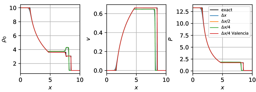
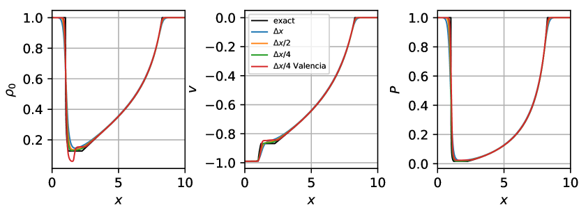
IV.1 Relativistic shock tube
This test is shown in Fig. 1. The left and right initial conditions we use for this evolution are , , respectively. The numerical solution in the Hamiltonian formulation is well-resolved, resulting in the three resolutions being difficult to distinguish. The contact discontinuity is not captured, since the pressure exhibits a jump there, whereas the only discontinuity should be in the rest mass density. The intermediate states to the left and right of the contact discontinuity at are also unphysical, as well as the shockwave speed.
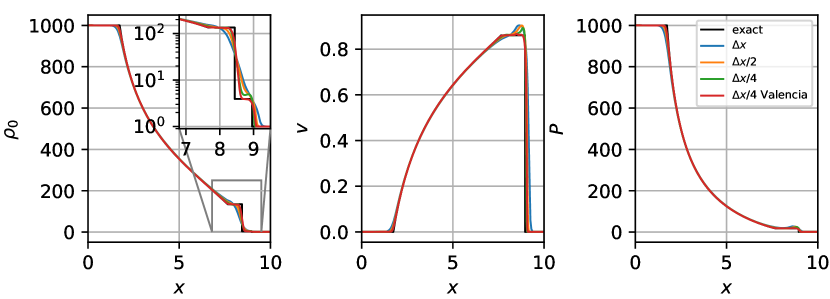
IV.2 Density discontinuity
This test is shown in Fig. 2. The left and right initial conditions we use for this evolution are , , respectively. The numerical solution in the Hamiltonian formulation is again well-resolved, and captures the exact solution well despite the very large initial discontinuity. However, the inset reveals a slightly incorrect density on the right side of the contact discontinuity.
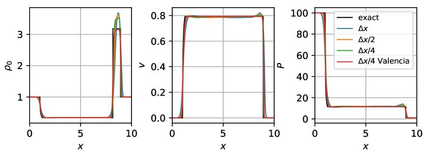
IV.3 Specific internal energy discontinuity
This test is shown in Fig. 3. The left and right initial conditions we use for this evolution are , , respectively. The intermediate state (corresponding to the “tower” feature in the density) is unphysical.
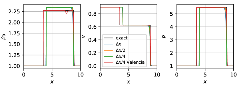
IV.4 Velocity discontinuity
We consider two cases with the initial velocity in the left state being rightwards and leftwards. The first case is shown in Fig. 4, whereby the left and right initial conditions we use for the rightwards evolution are , , respectively. The solution consists of a double shockwave, and the shockwave speeds and intermediate fluid state are seen to be unphysical. Resolving the intermediate state appears to be challenging for the Valencia scheme, where a dip in the density is exhibited near , which shrinks with increasing resolution.
For the leftwards evolution displayed in Fig. 5, we use , , respectively. The solution consists of a double rarefaction, and it is captured well in the Hamiltonian scheme. Rarefaction fans are captured well in a variety of formulations because the solution is continuous and isentropic across the fans Toro (2013); Martí and Müller (1994); Lora-Clavijo et al. (2013). But the Hamiltonian formulation we are using captures them particularly well, likely due to the fact that we are evolving the entropy density explicitly. The numerical Valencia solution actually performs worse, exhibiting a dip feature in the density near . This observation suggests that it may be beneficial in numerical applications to hybridize a numerical scheme to use Valencia near discontinuities, but evolve the entropy density otherwise.
V Conclusions
Hamiltonian formulations of fluid dynamics potentially offer unique advantages in numerical relativity, most of which are expected to be utilizable during the barotropic inspiral phase of a gravitational wave-driven binary coalescence involving at least one material body. The merger phase of the binary requires a baroclinic description. There are no advantages of using a Hamiltonian formulation over standard formulations that are currently apparent (although see Markakis et al. (2017)).
Nonetheless, the baroclinic case is worth consideration in order to obtain a better understanding of the limitations of Hamiltonian formulations in future applications. This work is part of a series of papers exploring the viability of such formulations in practice. We have considered a Hamiltonian formulation of baroclinic fluid dynamics, showing that it yields unphysical weak solutions under a path-conservative approximate Riemann solver scheme. Thus, in future implementations of Hamiltonian formulations in numerical relativity, an explicitly barotropic formulation is advised during the inspiral phase, and then switching to a standard baroclinic formulation prior to merger will be necessary. However, note that we have not excluded the possibility of obtaining physically correct weak solutions using the path through state space that is consistent with the viscosity solutions of the system, since we use only the linear path presented in Dumbser and Balsara (2016).
In the appendix we also point out that the barotropic Hamiltonian formulation admits shockwaves at fluid-vacuum interfaces, which may be related to the numerical instabilities observed at the stellar surface in Westernacher-Schneider et al. (2019). Those instabilities were dealt with via a hybrid Hamiltonian-Valencia scheme.
Acknowledgements.
We thank Charalampos Markakis, Vasileios Paschalidis, Eleuterio Toro, and Michael Dumbser for discussions. We give a special thanks to both Michael Dumbser and Dinshaw Balsara for providing code samples for the path-conservative HLL and HLLEM solvers in Dumbser and Balsara (2016), which greatly facilitated this work. This research is supported by National Science Foundation Grant No. PHY-1912619 at the University of Arizona.Appendix A Barotropic vacuum Riemann problem
It is well-known that the Newtonian vacuum Riemann problem results in a pure rarefaction adjacent to the vacuum (see e.g. Munz (1994); Munz et al. (1994); Toro (2013)). We can readily deduce the same conclusion in the special relativistic case using the jump conditions for the barotropic problem coming from conservation of rest mass and momentum,
| (34) | |||||
| (35) |
where is the shock speed, and the L and R subscripts denote the states to the left and right of the potential discontinuity. Setting the right state equal to vacuum, , which implies , the jump conditions reduce to
| (36) | |||||
| (37) |
Since the pressure in the fluid state vanishes, the pressure is therefore required to be continuous at the fluid vacuum interface. If the density must vanish along with the pressure (as per e.g. ), then the fluid-vacuum interface cannot support a discontinuity in the density either. Shockwaves are therefore not supported at fluid-vacuum interfaces. A rarefaction is the only other possible elementary wave in the barotropic case (and this is still true in the baroclinic case Munz (1994); Munz et al. (1994); Toro (2013)).
In the Hamiltonian formulation, the solution structure is different. Although all formulations agree in the rarefaction fan Toro (2013), they do not necessarily agree on whether or where the rarefaction fan terminates. Consider the jump conditions in the Hamiltonian formulation coming from conservation of rest mass and the Hamiltonian Euler equation,
| (38) | |||||
| (39) |
Setting the right state equal to vacuum yields
| (40) | |||||
| (41) |
or written another way,
| (42) | |||||
| (43) |
We see that the specific enthalpy can take on values greater than 1, implying a positive rest mass density. Rest mass discontinuities are therefore supported as shockwaves at fluid-vacuum interfaces in the Hamiltonian formulation. This may be related to the numerical instabilities found at the stellar surface in Westernacher-Schneider et al. (2019) when using a barotropic Hamiltonian formulation there.
Appendix B Convergence tests
To validate our numerical implementations, we performed independent residual tests on smooth numerical solutions. This means plugging the numerical solutions into the fluid equations in a separately coded script, and observing the rate of decrease of the residual as resolution is increased. An independent residual test is a form of analytic convergence test not requiring specific knowledge of an exact solution, other than the fact that the solution must obey the equations of motion.
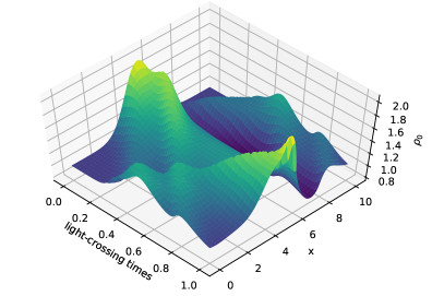
We use periodic boundary conditions on a domain length and a time step limitation . The initial conditions we use for this test are
| (44) | |||||
and the subsequent evolution of the rest mass density is depicted in Fig. 6. This depiction is intended to convey that this is a very dynamical evolution, and is therefore a non-trivial test of the numerical implementation. We evolve until 1 light-crossing time.
For two residuals and obtained at resolutions and , respectively, the global convergence factor is defined as
| (45) |
where we subjected the residuals to the -norm operator over space. The global convergence factor is a function of time, and its value is the convergence order measured in a spatially integrated sense.
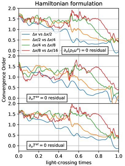
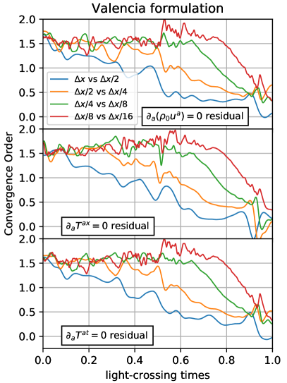
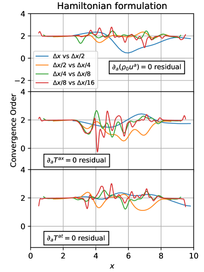
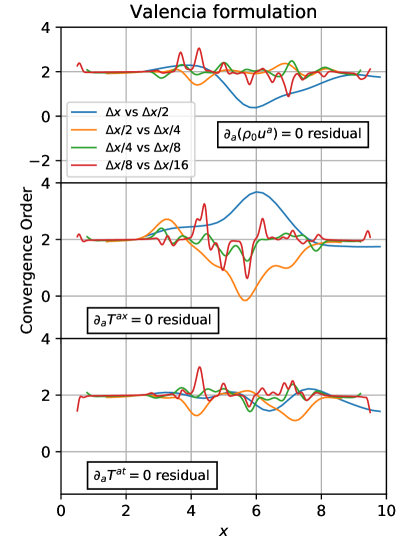
In Fig. 7 we display global convergence tests for the residuals of the fluid equations for both the Hamiltonian and Valencia formulations. The fiducial resolution is . The slope limiter deployed is the minmod type Toro (2013), and in the Hamiltonian formulation the slope limiter is also applied to the non-conservative product ( term in Eq. (30)), as per the numerical scheme in Dumbser and Balsara (2016). Both the Hamiltonian and Valencia formulations yield the expected 1.5th order global convergence for a nominally 2nd order finite volume scheme. However, the Euler equation residual in the Hamiltonian formulation suffers a somewhat diminished performance of 1st order during the first half of the evolution (Fig. 7, left middle panel). Based on our investigations, this diminished performance is due solely to the minmod-limited finite difference operator applied to the non-conservative term ( term in Eq. (30)) in the Hamiltonian Euler equation, as per Dumbser and Balsara (2016). Using instead a “monotonized central” limiter (MC limiter) Toro (2013) yields an improved convergence order of 1.5 (see Fig. 9). However, we find the MC limiter performs more poorly on shockwave solutions in comparison to the minmod limiter, therefore the shock tube evolutions we present in this work always use the minmod limiter.
As time proceeds, numerical truncation error builds up in the solutions. This manifests in the decreasing convergence order at later times. As resolution is increased, the expected 1.5th order convergence is maintained for longer durations of time.
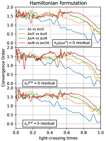
We also display the convergence order for the spatially local residual in Fig. 8. This is defined as
| (46) |
where now we evaluate the residual at the physical time corresponding to the first time step in the fiducial resolution , and take the absolute value rather than the -norm. The result is a function of spatial position, and indicates the instantaneous local convergence order. At such an early time, 2nd order convergence is obtained as expected.
References
- Aasi et al. (2015) J. Aasi, B. Abbott, R. Abbott, T. Abbott, M. Abernathy, K. Ackley, C. Adams, T. Adams, P. Addesso, R. Adhikari, et al., Classical and quantum gravity 32, 074001 (2015).
- Acernese et al. (2014) F. Acernese, M. Agathos, K. Agatsuma, D. Aisa, N. Allemandou, A. Allocca, J. Amarni, P. Astone, G. Balestri, G. Ballardin, et al., Classical and Quantum Gravity 32, 024001 (2014).
- Abbott et al. (2016a) B. P. Abbott, R. Abbott, T. Abbott, M. Abernathy, F. Acernese, K. Ackley, C. Adams, T. Adams, P. Addesso, R. Adhikari, et al., Physical review letters 116, 061102 (2016a).
- Abbott et al. (2017a) B. P. Abbott, R. Abbott, T. Abbott, F. Acernese, K. Ackley, C. Adams, T. Adams, P. Addesso, R. Adhikari, V. Adya, et al., Physical Review Letters 119, 161101 (2017a).
- Abbott et al. (2019a) B. Abbott, R. Abbott, T. Abbott, S. Abraham, F. Acernese, K. Ackley, C. Adams, R. Adhikari, V. Adya, C. Affeldt, et al., Physical Review X 9, 031040 (2019a).
- Abbott et al. (2017b) B. P. Abbott, R. Abbott, T. Abbott, M. Abernathy, F. Acernese, K. Ackley, C. Adams, T. Adams, P. Addesso, R. Adhikari, et al., Classical and Quantum Gravity 34, 104002 (2017b).
- Haster et al. (2016) C.-J. Haster, Z. Wang, C. P. Berry, S. Stevenson, J. Veitch, and I. Mandel, Monthly Notices of the Royal Astronomical Society 457, 4499 (2016).
- Buonanno and Damour (1999) A. Buonanno and T. Damour, Physical Review D 59, 084006 (1999).
- Husa et al. (2016) S. Husa, S. Khan, M. Hannam, M. Pürrer, F. Ohme, X. J. Forteza, and A. Bohé, Physical Review D 93, 044006 (2016).
- Boyle et al. (2019) M. Boyle, D. Hemberger, D. A. Iozzo, G. Lovelace, S. Ossokine, H. P. Pfeiffer, M. A. Scheel, L. C. Stein, C. J. Woodford, A. B. Zimmerman, et al., Classical and Quantum Gravity 36, 195006 (2019).
- Dietrich et al. (2018) T. Dietrich, D. Radice, S. Bernuzzi, F. Zappa, A. Perego, B. Brügmann, S. V. Chaurasia, R. Dudi, W. Tichy, and M. Ujevic, Classical and Quantum Gravity 35, 24LT01 (2018).
- Haas et al. (2016) R. Haas, C. D. Ott, B. Szilagyi, J. D. Kaplan, J. Lippuner, M. A. Scheel, K. Barkett, C. D. Muhlberger, T. Dietrich, M. D. Duez, et al., Physical Review D 93, 124062 (2016).
- Kiuchi et al. (2017) K. Kiuchi, K. Kawaguchi, K. Kyutoku, Y. Sekiguchi, M. Shibata, and K. Taniguchi, Physical Review D 96, 084060 (2017).
- Abbott et al. (2016b) B. P. Abbott, R. Abbott, T. D. Abbott, M. Abernathy, F. Acernese, K. Ackley, C. Adams, T. Adams, P. Addesso, R. X. Adhikari, et al., Physical Review X 6, 041014 (2016b).
- Abbott et al. (2019b) B. Abbott, R. Abbott, T. Abbott, F. Acernese, K. Ackley, C. Adams, T. Adams, P. Addesso, R. Adhikari, V. Adya, et al., Physical Review X 9, 011001 (2019b).
- Abbott et al. (2017c) B. P. Abbott, R. Abbott, T. Abbott, M. Abernathy, K. Ackley, C. Adams, P. Addesso, R. Adhikari, V. Adya, C. Affeldt, et al., Classical and Quantum Gravity 34, 044001 (2017c).
- Reitze et al. (2019) D. Reitze, R. X. Adhikari, S. Ballmer, B. Barish, L. Barsotti, G. Billingsley, D. A. Brown, Y. Chen, D. Coyne, R. Eisenstein, et al., arXiv preprint arXiv:1907.04833 (2019).
- Samajdar and Dietrich (2018) A. Samajdar and T. Dietrich, Physical Review D 98, 124030 (2018).
- Samajdar and Dietrich (2019) A. Samajdar and T. Dietrich, Physical Review D 100, 024046 (2019).
- Brown (2020) D. Brown, Bulletin of the American Physical Society (2020).
- Goldberger and Rothstein (2006) W. D. Goldberger and I. Z. Rothstein, Physical Review D 73, 104029 (2006).
- Galley and Tiglio (2009) C. R. Galley and M. Tiglio, Physical Review D 79, 124027 (2009).
- Blanchet (2014) L. Blanchet, Living Reviews in Relativity 17, 2 (2014).
- Bini et al. (2020a) D. Bini, T. Damour, and A. Geralico, arXiv preprint arXiv:2003.11891 (2020a).
- Bini et al. (2020b) D. Bini, T. Damour, and A. Geralico, arXiv preprint arXiv:2004.05407 (2020b).
- Nagar and Rettegno (2019) A. Nagar and P. Rettegno, Physical Review D 99, 021501 (2019).
- Blümlein et al. (2020) J. Blümlein, A. Maier, P. Marquard, and G. Schäfer, arXiv preprint arXiv:2003.01692 (2020).
- Landry and Poisson (2015) P. Landry and E. Poisson, Physical Review D 91, 104018 (2015).
- Landry (2017) P. Landry, Physical Review D 95, 124058 (2017).
- Pani et al. (2015a) P. Pani, L. Gualtieri, and V. Ferrari, Physical Review D 92, 124003 (2015a).
- Pani et al. (2015b) P. Pani, L. Gualtieri, A. Maselli, and V. Ferrari, Physical Review D 92, 024010 (2015b).
- Steinhoff et al. (2016) J. Steinhoff, T. Hinderer, A. Buonanno, and A. Taracchini, Physical Review D 94, 104028 (2016).
- Lim et al. (2015) D.-J. Lim, T. R. Anderson, and T. Shott, Omega 51, 128 (2015).
- Stevens et al. (2019) R. Stevens, J. Ramprakash, P. Messina, M. Papka, and K. Riley, Aurora: Argonne’s Next-Generation Exascale Supercomputer, Tech. Rep. (ANL (Argonne National Laboratory (ANL), Argonne, IL (United States)), 2019).
- Narasimhamurthy et al. (2019) S. Narasimhamurthy, N. Danilov, S. Wu, G. Umanesan, S. Markidis, S. Rivas-Gomez, I. B. Peng, E. Laure, D. Pleiter, and S. De Witt, Parallel Computing 83, 22 (2019).
- Kidder et al. (2017) L. E. Kidder, S. E. Field, F. Foucart, E. Schnetter, S. A. Teukolsky, A. Bohn, N. Deppe, P. Diener, F. Hébert, J. Lippuner, et al., Journal of Computational Physics 335, 84 (2017).
- Palenzuela et al. (2018) C. Palenzuela, B. Miñano, D. Viganò, A. Arbona, C. Bona-Casas, A. Rigo, M. Bezares, C. Bona, and J. Massó, Classical and Quantum Gravity 35, 185007 (2018).
- Zhang et al. (2019) W. Zhang, A. Almgren, V. Beckner, J. Bell, J. Blaschke, C. Chan, M. Day, B. Friesen, K. Gott, D. Graves, et al., Journal of Open Source Software 4 (2019).
- Fernando et al. (2018) M. Fernando, D. Neilsen, H. Lim, E. Hirschmann, and H. Sundar, arXiv preprint arXiv:1807.06128 (2018).
- Neilsen et al. (2019) D. Neilsen, M. Fernando, H. Sundar, and E. Hirschmann, Bulletin of the American Physical Society 64 (2019).
- Radice et al. (2013) D. Radice, L. Rezzolla, and F. Galeazzi, Monthly Notices of the Royal Astronomical Society: Letters 437, L46 (2013).
- Miller and Schnetter (2016) J. M. Miller and E. Schnetter, Classical and Quantum Gravity 34, 015003 (2016).
- Bugner et al. (2016) M. Bugner, T. Dietrich, S. Bernuzzi, A. Weyhausen, and B. Brügmann, Physical Review D 94, 084004 (2016).
- Bernuzzi and Dietrich (2016) S. Bernuzzi and T. Dietrich, Physical Review D 94, 064062 (2016).
- Felker and Stone (2018) K. G. Felker and J. M. Stone, Journal of Computational Physics 375, 1365 (2018).
- Foucart et al. (2019) F. Foucart, M. Duez, A. Gudinas, F. Hébert, L. Kidder, H. Pfeiffer, and M. Scheel, Physical Review D 100, 104048 (2019).
- Most et al. (2019) E. R. Most, L. J. Papenfort, and L. Rezzolla, Monthly Notices of the Royal Astronomical Society 490, 3588 (2019).
- Fambri et al. (2018) F. Fambri, M. Dumbser, S. Köppel, L. Rezzolla, and O. Zanotti, Monthly Notices of the Royal Astronomical Society 477, 4543 (2018).
- Fambri (2020) F. Fambri, Archives of Computational Methods in Engineering 27, 199 (2020).
- Köppel (2018) S. Köppel, in Journal of Physics: Conference Series, Vol. 1031 (IOP Publishing, 2018) p. 012017.
- Ruchlin et al. (2018a) I. Ruchlin, Z. B. Etienne, and T. W. Baumgarte, Physical Review D 97, 064036 (2018a).
- Ruchlin et al. (2018b) I. Ruchlin, Z. B. Etienne, and T. W. Baumgarte, Astrophysics Source Code Library (2018b).
- Synge (1937) J. L. Synge, Proc. Lond. Math. Soc. 43, 376 (1937).
- Lichnerowicz (1941) A. Lichnerowicz, in Annales scientifiques de l’École Normale Supérieure, Vol. 58 (1941) pp. 285–304.
- Markakis (2014) C. M. Markakis, arXiv preprint arXiv:1410.7777 (2014).
- Markakis et al. (2017) C. Markakis, K. Uryū, E. Gourgoulhon, J.-P. Nicolas, N. Andersson, A. Pouri, and V. Witzany, Physical Review D 96, 064019 (2017).
- Westernacher-Schneider et al. (2019) J. R. Westernacher-Schneider, C. Markakis, and B. J. Tsao, arXiv preprint arXiv:1912.03701 (2019).
- Rieutord et al. (2006) M. Rieutord, B. Dubrulle, and E. Gourgoulhon, European Astronomical Society Publications Series 21, 43 (2006).
- Friedman and Stergioulas (2013) J. L. Friedman and N. Stergioulas, Rotating relativistic stars (Cambridge University Press, 2013).
- Kelvin (1869) L. Kelvin, Trans. Roy. Soc. Edinb. 25, 217 (1869).
- Brodbeck et al. (1999) O. Brodbeck, S. Frittelli, P. Hübner, and O. A. Reula, Journal of Mathematical Physics 40, 909 (1999).
- Gundlach et al. (2005) C. Gundlach, G. Calabrese, I. Hinder, and J. M. Martín-García, Classical and Quantum Gravity 22, 3767 (2005).
- Banyuls et al. (1997) F. Banyuls, J. A. Font, J. M. Ibáñez, J. M. Martí, and J. A. Miralles, The Astrophysical Journal 476, 221 (1997).
- Vol’pert (1967) A. I. Vol’pert, Matematicheskii Sbornik 115, 255 (1967).
- Cauret et al. (1989) J.-J. Cauret, J.-F. Colombeau, and A. Le Roux, Journal of mathematical analysis and applications 139, 552 (1989).
- Dal Maso et al. (1995) G. Dal Maso, P. G. Lefloch, and F. Murat, Journal de mathématiques pures et appliquées 74, 483 (1995).
- Díaz et al. (2008) M. C. Díaz, E. D. Fernández-Nieto, and A. Ferreiro, Computers & Fluids 37, 299 (2008).
- Pelanti et al. (2008) M. Pelanti, F. Bouchut, and A. Mangeney, ESAIM: Mathematical Modelling and Numerical Analysis 42, 851 (2008).
- Fernández-Nieto et al. (2008) E. D. Fernández-Nieto, F. Bouchut, D. Bresch, M. C. Diaz, and A. Mangeney, Journal of Computational Physics 227, 7720 (2008).
- Munkejord et al. (2009) S. T. Munkejord, S. Evje, and T. FlÅtten, SIAM Journal on Scientific Computing 31, 2587 (2009).
- Morales de Luna et al. (2009) T. Morales de Luna, M. J. Castro Díaz, C. Parés Madroñal, and E. D. Fernández Nieto, Communications in computational physics, 6 (4), 848-882. (2009).
- Dumbser and Toro (2011) M. Dumbser and E. F. Toro, Journal of Scientific Computing 48, 70 (2011).
- Müller et al. (2013) L. O. Müller, C. Parés, and E. F. Toro, Journal of Computational Physics 242, 53 (2013).
- Fernández-Nieto et al. (2014) E. D. Fernández-Nieto, J. M. Gallardo, and P. Vigneaux, Journal of Computational Physics 264, 55 (2014).
- Díaz et al. (2014) M. C. Díaz, E. D. Fernández-Nieto, G. Narbona-Reina, and M. de la Asunción, Journal of Computational Physics 262, 172 (2014).
- Sánchez-Linares et al. (2016) C. Sánchez-Linares, T. M. de Luna, and M. C. Díaz, Applied Mathematics and Computation 272, 369 (2016).
- Castro et al. (2017) M. J. Castro, T. M. de Luna, and C. Parés, in Handbook of Numerical Analysis, Vol. 18 (Elsevier, 2017) pp. 131–175.
- Dumbser and Balsara (2016) M. Dumbser and D. S. Balsara, Journal of Computational Physics 304, 275 (2016).
- dum (2019) Private communication with Michael Dumbser (2019).
- Toro (2013) E. F. Toro, Riemann solvers and numerical methods for fluid dynamics: a practical introduction (Springer Science & Business Media, 2013).
- Alcubierre (2008) M. Alcubierre, Introduction to 3+1 Numerical Relativity, International Series of Monographs on Physics (OUP Oxford, 2008).
- Schwabl (2006) F. Schwabl, stme (2006).
- Harten et al. (1983) A. Harten, P. D. Lax, and B. v. Leer, SIAM review 25, 35 (1983).
- Giacomazzo and Rezzolla (2006) B. Giacomazzo and L. Rezzolla, Journal of Fluid Mechanics 562, 223 (2006).
- (85) https://www.brunogiacomazzo.org/?page_id=395.
- Martí and Müller (1994) J. M. Martí and E. Müller, Journal of Fluid Mechanics 258, 317 (1994).
- Lora-Clavijo et al. (2013) F. Lora-Clavijo, J. Cruz-Pérez, F. Siddhartha Guzmán, and J. González, Revista mexicana de física E 59, 28 (2013).
- Munz (1994) C.-D. Munz, Mathematical methods in the applied sciences 17, 597 (1994).
- Munz et al. (1994) C.-D. Munz, R. Schneider, and O. Gerlinger, in Numerical methods for the Navier-Stokes equations (Springer, 1994) pp. 181–190.