Using Decision Diagrams to Compactly Represent the State Space for Explicit Model Checking

Abstract

The enormous number of states reachable during explicit model checking is the main bottleneck for scalability. This paper presents approaches of using decision diagrams to represent very large state space compactly and efficiently. This is possible for asynchronous systems as two system states connected by a transition often share many same local portions. Using decision diagrams can significantly reduce memory demand by not using memory to store the redundant information among different states. This paper considers multi-value decision diagrams for this purpose. Additionally, a technique to reduce the runtime overhead of using these diagrams is also described. Experimental results and comparison with the state compression method as implemented in the model checker SPIN show that the approaches presented in this paper are memory efficient for storing large state space with acceptable runtime overhead.

I Introduction

Model checking [8] is an automated formal analysis method for verifying hardware and software systems. It systematically checks whether a model of a given system satisfies a desired property such as deadlock freedom and request-response properties [5]. However, model checking is computationally very expensive as it searches the entire reachable state space of a design for errors. Typically, all reachable states found during reachability analysis need to be stored to avoid searching the same part of state space multiple times unnecessarily. As the number of states grows exponentially in the size of designs under verification, physical memory installed on typical computers can be exhausted quickly, therefore limiting model checking to the designs of small sizes. This problem is well known as state explosion.

In asynchronous designs, multiple components execute concurrently. When verifying asynchronous designs, generally interleaving semantics are used to represent the behavior of such designs. More specifically, when multiple components are ready to execute in a state, only one component is selected. This interleaved execution makes sure all possible orderings of concurrently enabled executions are considered, thus capturing all possible behavior for verification. The need to consider all possible interleavings of concurrent executions is the main cause of state explosion in asynchronous design verification as the number of interleavings grows exponentially if a design has a high degree of concurrency, and this leads to an excessively large state space for even a relatively small system.

In the interleaved execution as described above, only one component executes and updates the relative portion of a state, and the remaining portions of the state are unchanged. Therefore, storing the entire states results in unnecessary overhead. In model checker SPIN [12], a state compression method is described where the independent parts of the design states are considered when representing states. Independent parts refer to variables including global and local variables belonging to different processes. An unique copy is created for each different independent part, and the references to the copies of independent parts are used to construct the states.

While the above compression method reduces memory significantly in representing states, there are still a lot of redundancies in the state representations. As pointed out in the previous paragraphs, a global state of a design is in fact a tuple of pointers to the local states. Two states connected by a state transition may still share a large number of same pointers in their representations as a state transition typically causes only a few local changes. Therefore, reducing the redundancy in the state representations further can improve the scalability even more. This paper proposes to use the multi-value decision diagrams to represent the reachable states for explicit model checking of asynchronous systems. The multi-value decision diagrams, similar to the well-known binary decision diagrams (BDD) [3], uses directed acyclic graphs to sets of objects encoded by typed variables. The compactness of the decision diagram representations is due to sharing of common portions of a large number of different objects.

BDDs are widely used in symbolic model checking [4] where the model checking algorithms and the state representations are both based on the Boolean operations. However, in the explicit model checking, individual states are created and manipulated. Adding individual states into a decision diagram representation can incur high runtime overhead, and this would cancel largely the benefit of compact memory footprint of the decision diagrams. To address this problem, this paper also proposes to use multi-value decision trees along with the decision diagrams. Adding states into a decision tree is much faster, but it requires more memory than a decision diagram. In this method, a decision tree is used as a buffer where it stores the reachable states until some threshold is exceeded. Then, the decision tree is compressed, and merged with the decision diagram representing the whole reachable state space. This approach can significantly reduce the runtime overhead associated with using the decision diagrams, even though it may increase the average memory required compared to using the decision diagrams solely.

In this paper, the multi-value decision diagrams are only used to store the states found during the depth-first search that are generally implemented for the explicit model checking of asynchronous systems. The algorithms themselves remain the same. Therefore, the previous results to improve scalability such as partial order reduction [9, 10] can still be used.

The idea of using graph representation to store reachable states is previously described in [11] where a finite automaton is used. As indicated in [11], this approach has very high overhead to use. This paper addresses that problem by using a decision tree as a buffer to reduce such overhead. Using multi-value decision diagrams for storing states is also described in [6]. There are two main differences between this work and that in [6]. First, the Petri-net models used in [6] are different from the model used in this work where in this paper Petri-net transitions are labeled with additional state space information. Second, [6] uses an exotic search strategy to achieve high memory efficiency. However, this work uses multi-value decision diagrams to store reachable states without altering the depth-first search framework, therefore partial order reduction can be easily integrated.

II Background

II-A Labeled Petri-Nets

This paper uses Labeled Petri-Nets to model asynchronous systems. Petri-Nets are a common modeling formalism for asynchronous designs [14, 1]. A Petri-net is a directed graph with a set of transitions and a set of places. A labeled Petri-Net is a Petri-net where transitions are labeled with various information representing a system’s properties and behavior [17]. Its definition is given as follows.

Definition II.1

A labeled Petri-net (LPN) is a tuple $N=\langle V,P,T,F,\mu_{0},\alpha_{0},L\rangle$,where

1. $V$ is a set of state variables of the integer type,

2. $P$ is a finite set of places,

3. $T$ is a finite set of transitions,

4. $F\subseteq(P\times T)\cup(T\times P)$ is a finite set of the flow relations,

5. $\mu_{0}\subseteq P$ is a finite set of initially marked places,

6. $\alpha_{0}:V\rightarrow\mathbb{Z}$ is a labeling function that assigns each variable an initial value,

7. $L=\langle Guard,Assign\rangle$ is a pair of labeling functions for transitions in $T$, which is defined below.

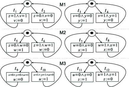
(a)	(b)

Figure 1: (a) A simple asynchronous circuit. (b) The LPNs for module $M_{1}$, $M_{2}$, and $M_{3}$. The initial values of variables $u$, $v$, $w$, $x$, $y$, and $z$ are $0$, $1$, $1$, $0$, $0$, and $0$, respectively.

A simple LPN example is shown in Fig 1. Fig.1(a) shows a simple asynchronous circuit consisting of three components, and Fig. 1(b) shows the LPNs for each component in the circuit. For each component, its LPN has 2 places and 4 transitions. The places are represented as circles, and the transitions are represented as boxes. Each place is preceded and followed by one or more transitions, and each transition is preceded and followed by one or more places. The flow relations are represented by the edges connecting the transitions and places [1]. The bullets found in some places are called tokens. Each place can have at most one token. A place is marked if it has a token. A marking of LPN, $\mu\subseteq P$ is a set of marked places.

The dynamic behavior of a concurrent system is captured by LPN transitions with labelings. Each transition $t\in T$ has a $preset$ denoted by $\bullet t=\{p\in P|(p,t)\in F\}$, which is the set of places connected to $t$, and a $postset$ denoted by $t\bullet=\{p\in P|(t,p)\in F\}$, which is the set of places to which $t$ is connected. The $preset$ and $postset$ for places are defined similarly.

Before defining the transition labels formally, the grammar used by these labels is introduced first below [17]. The numerical portion of the grammar is defined as follows:

$$\chi ::= c_{i}~{}|~{}v_{i}~{}|~{}(\chi)~{}|~{}-\chi~{}|~{}\chi+\chi~{}|~{}\chi-\chi~{}|~{}\chi*\chi~{}|$$

$$\chi/\chi~{}|~{}\chi\verb!^!\chi~{}|~{}\chi\%\chi~{}|~{}\textup{NOT}(\chi)~{}|~{}\textup{OR}(\chi,\chi)~{}|$$

$$\textup{AND}(\chi,\chi)~{}|~{}\textup{XOR}(\chi,\chi)~{}|~{}\textup{INT}(\phi)$$

where $c_{i}$ is an integer constant from ${\mathbb{Z}}$, and $v_{i}$ is an integer variable. The functions NOT, OR, AND, and XOR are bit-wise logical operations assuming a 2’s complement format with arbitrary precision. $\textup{INT}(\phi)$ returns $1$ if the Boolean expression $\phi$, which is defined below, evaluates to true, or $0$ otherwise. The set $\mathcal{P_{\chi}}$ is defined to be all formulas that can be constructed from the $\chi$ grammar.

The Boolean portion of the grammar is as follows:

$$\phi ::= \textbf{true}~{}|~{}\textbf{false}~{}|~{}v_{i}~{}|~{}\neg\phi~{}|~{}\phi\wedge\phi~{}|~{}\phi\vee\phi~{}|~{}\chi\equiv\chi~{}|$$

$$\chi\geq\chi~{}|~{}\chi>\chi~{}|~{}\chi\leq\chi~{}|~{}\chi<\chi$$

where the integer $v_{i}$ is regarded as true if its value is nonzero, and false otherwise. In this sense, it is similar to the semantics of the C language. The set $\mathcal{P_{\phi}}$ is defined to be all formulas that can be constructed from the $\phi$ grammar.

As in Definition II.1, each LPN transition is labeled with an enabling condition and a set of variable assignments. LPN transition labeling is defined by $L=\langle Guard,Assign\rangle$ where

• $Guard:T\rightarrow\mathcal{P_{\phi}}$ labels each LPN transition with a Boolean expression that defines its enabling condition.

• $Assign:T\times V\rightarrow\mathcal{P_{\chi}}$ labels each LPN transition $t\in T$ and each variable $v\in V$ with an integer assignment made to $v$ when $t$ fires.

For a large complex design, it usually consists of multiple components. Then, each component is modeled in a LPN module, and the LPN for the whole design is the parallel composition of the LPN modules. Let $N_{1}$, $\ldots$, $N_{n}$ be the LPN modules for the components consisting of a design. The LPN for the design is $N=N_{1}\|\ldots\|N_{n}$ where $\|$ is the parallel composition operator for LPNs. In our method, communications among components are represented by the shared variables. Shared variables between components $N_{i}$ and $N_{j}$ are variables in $V_{i}\cap V_{j}$. Moreover, no two LPN modules share any common places. In other words, $\forall_{i,j}i\not=j\Rightarrow P_{i}\cap P_{j}=\emptyset$. In Fig. 1, the design is partitioned into three components for illustration purpose. These components are represented by LPN modules as shown in $M_{1}$, $M_{2}$, and $M_{3}$.

II-B Reachability Analysis

A basic approach for analyzing the dynamic behavior of a concurrent system modeled with LPNs is reachability analysis, which finds all possible state transitions and thus reachable states for such a system. The reachable state space is typically represented by a state graph. A state graph is a directed graph where vertices represent states and edges represent state transitions.

A state of a LPN module $N_{i}$ is a pair $(\mu_{i},\sigma_{i})$ where $\mu_{i}$ denotes a marking of $N_{i}$ and $\sigma_{i}$ denotes a vector of values over variables $V_{i}$ of $N_{i}$. The initial state $init$ of $N_{i}$ is $(\mu_{0},\alpha_{0})$. Given a state $s_{i}$ of module $N_{i}$, $M(s_{i})$ denotes the marking of $s_{i}$ and $\sigma(s_{i})$ denotes the state vector of $s_{i}$. Also, for any expression $e\in\mathcal{P_{\chi}}\cup\mathcal{P_{\phi}}$, $value(e,s_{i})$ denotes a function that returns the value of expression $e$ in state $s_{i}$. As described in the previous section, the LPN of a design is the parallel composition of a set of LPN modules, each of which represents a component in the design. Let $N=N_{1}\|\ldots\|N_{n}$ be the LPN of a design where $N_{i}~{}(1\leq i\leq n)$ is the LPN module for the $i$th component of the design. A global state $\vec{s}\hskip 2.0pt$ of $N$ is a $n$-tuple $(s_{1},\ldots,s_{n})$ where each $s_{i}~{}(1\leq i\leq n)$ is a local state of LPN module $N_{i}$.

Before describing the reachability analysis, the enabling condition of the LPN transitions is defined below.

Definition II.2

Let $N_{i}$ be a LPN module. A LPN transition $t$ is enabled in a state $s$ if the following two conditions are met:

1. $\bullet t\subseteq\mu(s)$,

2. $value(e,s)$ is $true$ or not zero for $e=Guard(t)$.

In Fig 1, every transition has its preset included in the initial marking. In the initial state, the values of variable $u$ and $z$ are $0$, $Guard(t_{11})$, which is $u=0\wedge z=0$, is evaluated to be true, therefore transition $t_{11}$ is enabled in the initial state.

Given a LPN module, the set of transitions enabled in a state $s$ is denoted by $enabled(s)$. Naturally, the enabled transitions of the whole design LPN is denoted by $enabled(\vec{s}\hskip 2.0pt)$. The reachable state space of a LPN model can be found by exhaustively firing every enabled transition starting at the initial state. Firing a transition may lead to a new state by generating a new marking and a new state vector according to the assignments labeled for such transition. Detailed definition of transition firing can be found in [1]. In this paper, $s^{\prime}=t(s)$ denotes that a new state $s^{\prime}$ is produced by firing transition $t$ in state $s$ in a LPN module. Similarly, $\vec{s}\hskip 2.0pt^{\prime}=t(\vec{s}\hskip 2.0pt)$ denotes that a new global state $\vec{s}\hskip 2.0pt^{\prime}$ is produced by firing transition $t$ in global state $\vec{s}\hskip 2.0pt$.

$stateTable.add(\vec{s}\hskip 2.0pt_{0})$;

$stateStack.push(\vec{s}\hskip 2.0pt_{0})$;

$enabledStack.push(enabled(\vec{s}\hskip 2.0pt_{0}))$;

while stack is not empty do $\vec{s}\hskip 2.0pt=stateStack.top()$;

$E_{\vec{s}\hskip 2.0pt}=enabledStack.top()$;

if $E_{\vec{s}\hskip 2.0pt}=\emptyset$ then $stateStack.pop()$;

$enabledStack.pop()$;

continue;

Select $t\in E_{\vec{s}\hskip 2.0pt}$ to fire;

$E_{\vec{s}\hskip 2.0pt}=E_{\vec{s}\hskip 2.0pt}\backslash t$;

$\vec{s}\hskip 2.0pt^{\prime}=t(\vec{s}\hskip 2.0pt)$;

if $stateTable.contains(\vec{s}\hskip 2.0pt)=={\bf true}$ then $stateStack.push(\vec{s}\hskip 2.0pt^{\prime})$;

$enabledStack.push(enabled(\vec{s}\hskip 2.0pt^{\prime}))$;

$stateTable.add(\vec{s}\hskip 2.0pt^{\prime})$;

Algorithm 1 $search((T,P,F,M_{0}))$

14

14

14

14

14

14

14

14

14

14

14

14

14

14

The procedure to find the reachable state space of a given LPN model is given in Algorithm 1. Reachable states are stored in stateTable. During the reachability analysis, after a LPN transition $t_{i}$ is fired in global state $\vec{s}\hskip 2.0pt$, the local state of $M_{i}$ is changed to a new one. In other words, if transition $t_{i}$ is fired in state $\vec{s}\hskip 2.0pt=(s_{1},\ldots,s_{i},\ldots,s_{n})$, a new global state $\vec{s}\hskip 2.0pt^{\prime}$ is generated such that $\vec{s}\hskip 2.0pt^{\prime}=(s^{\prime}_{1},\ldots,s^{\prime}_{i},\ldots,s^{\prime}_{n})$. Observe that in $\vec{s}\hskip 2.0pt$ and $\vec{s}\hskip 2.0pt^{\prime}$, many local states might be exactly the same. To avoid creating fresh copies of the same local states for $\vec{s}\hskip 2.0pt^{\prime}$ in memory, the actual definitions of the distinct local states are stored in a hash table for each LPN module, and the pointers to the local states are used to construct the global states. From now on, $\vec{s}\hskip 2.0pt=(s_{1},\ldots,s_{n})$ is viewed as a tuple of pointers to the local states $s_{i},\ldots$, and $s_{n}$. In this way, a local state is created only once, and its pointer may be referenced many times in different global states. The similar state representation is also implemented in the model checker SPIN [12] and Java PathFinder [2].

In many existing model checkers, the obvious choice of the data structure for $stateTable$ is hash tables. Even though inserting and accessing hash tables are usually very efficient, the memory usage increases exponentially as the number of states found during the reachability analysis increases exponentially in the size of a design. Therefore, representing and storing reachable states compactly is extremely important. To address this problem, the following sections describe how the reachable states are represented using graphs, specifically decision trees and diagrams which may allow very large number of states to be stored in a relatively small memory footprint.

III State Space Representations

As described above, different global states might have a large number of pointers to the same local states. To save memory even further by avoiding storing the same local state pointers in different global states, a data structure called multi-value decision diagram (MDD) is implemented in our method to store global states found during the reachability analysis. The concept of MDD [19] is very close to that of binary decision diagrams (BDDs) [3] in that both use graphs to represent a set of objects encoded by some variables. The memory efficiency comes from the sharing of the same variables used to encode different objects. In BDDs, the variables used for the encoding are binary variables, while integer variables are used for the encoding in the case of MDDs. In this sense, BDDs can be regarded as a special case of MDDs. The structural representation of the global states in our method is natural for MDDs. To facilitate the presentation, an unique integer index is assigned to each local state of a single LPN module. Therefore, a global state $\vec{s}\hskip 2.0pt=(s_{1},\ldots,s_{n})$ can be regarded as a tuple of integers where $s_{i}$ is the index to a local state of module $i$.

III-A Multi-Value Decision Trees

This section describes multi-value decision trees to introduce multi-value decision diagrams that are described in the next section. A multi-value decision tree is a directed acyclic graph with a single root node, terminal nodes and non-terminal nodes. The root node does not have incoming edges, and the terminal nodes do not have any outgoing edges. Each non-terminal node has a single incoming edge and one or more outgoing edges. Each edge is labeled with an integer number. A path is a sequence of edges from the root to one of the terminal nodes, therefore an integer tuple can be formed by collecting the integers labeled on the edges on the path. In other words, a path represents or encodes an integer tuple. An example of multi-value decision tree is shown in Fig. 2. Note that a terminal node is drawn for each path in the figure to make presentation clear. In the actual implementation, only a single terminal node is used, and all paths converge to this unique terminal node.

$\displaystyle(0,0,0)$ $\displaystyle(0,0,1)$ $\displaystyle(0,1,0)$ $\displaystyle(0,1,1)$ $\displaystyle(1,1,1)$ $\displaystyle(1,1,2)$
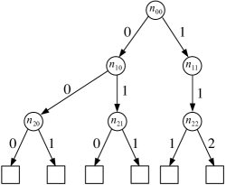
(a)	(b)

Figure 2: (a) A set of integer triples, (b) The corresponding multi-value decision tree representation for the set shown in (a).

In our implementation, two operations are supported for multi-value decision tree, add and contains. Function add takes as input an integer tuple, and creates necessary edges in the decision tree to build a path corresponding to the input tuple. For example shown in Fig. 2, if a new tuple $(1,1,3)$ is given, it can be added to the decision tree by creating an edge from node $n_{21}$ to the terminal node, and this edge is labeled with $3$. If another tuple $(1,1,1)$ is given, then no new edge is created as there is a path existing in the decision tree corresponding to the given tuple. Function contains also takes as input an integer tuple, and checks if there is a path in the decision tree that corresponds to the given tuple. It returns true if there is, false otherwise. The time complexity of both functions is linear in the size of the tuples.

The memory efficiency of the decision trees depends on the similarity of the prefixes of the tuples in the given set. If there are a large number of tuples with long same prefixes, a lot of node sharing can reduce the memory usage significantly. On the other hand, the worst case happens when a large number of tuples differ on their first elements. In this case, more memory may be required compared to using hash tables as an edge is needed for each element in each tuple.

III-B Multi-Value Decision Diagrams

A multi-value decision diagram, similar to the decision trees, is a rooted directed acyclic graph where there is an unique root node, an unique terminal node, and non-terminal nodes. In a multi-value decision diagram, the nodes are partitioned into levels. The number of levels of a decision diagram is equal to the size of the integer tuples representing the global states. The root node is at level 0, which is at the top of the decision diagram. The node at the bottom is the terminal. Each non-terminal node has a number of outgoing edges connecting nodes at one level higher or the terminal, and a number of incoming edges from nodes including the root node from one level lower. Non-terminal nodes in the decision diagrams, unlike those in the decision trees, can have multiple incoming and outgoing edges. A path from the root node to the terminal node in a decision diagram corresponds an integer tuple. In the reachability analysis, the decision diagrams are used to replace the hash tables, therefore our implementation only supports two operations, union and contains. Since contains for the decision diagrams is the same as function contains for the decision trees, union is described in this section.

Function union takes as inputs two decision diagrams, and returns a decision diagram that includes all the paths from either of the two input decision diagrams. During the union operation, an unique table is maintained to make sure that no equivalent nodes are created. Before the node equivalence is defined, let $(n,i,n^{\prime})$ be an outgoing edge of node $n$, and the set of all outgoing edges of node $n$ is denoted as $outgoing(n)$. Two nodes $n_{1}$ and $n_{2}$ are equivalent, denoted as $n_{1}\equiv n_{2}$, if $n_{1}$ and $n_{2}$ are the same, or the following conditions are satisfied.

• $\forall_{(n_{1},i,n^{\prime}_{1})}\exists_{(n_{2},i,n^{\prime}_{2})}~{}n^{\prime}_{1}\equiv n^{\prime}_{2}$.

• $\forall_{(n_{2},j,n^{\prime}_{2})}\exists_{(n_{1},j,n^{\prime}_{1})}~{}n^{\prime}_{1}\equiv n^{\prime}_{2}$.

Function union creates a new decision diagram for two input diagrams as follows. Starting from the root nodes $n_{1}$ and $n_{2}$ of the two input decision diagrams, it creates a new node $n$ by following the rules shown below.

1. For each edge ${(n_{1},i,n^{\prime}_{1})}\in outgoing(n_{1})$, if there is no ${(n_{2},i,n^{\prime}_{2})}$ in $outgoing(n_{2})$, add $(n,i,n^{\prime}_{1})$ to $outgoing(n)$.

2. For each edge ${(n_{2},i,n^{\prime}_{2})}\in outgoing(n_{2})$, if there is no ${(n_{1},i,n^{\prime}_{1})}$ in $outgoing(n_{1})$, add $(n,i,n^{\prime}_{2})$ to $outgoing(n)$.

3. For each edge ${(n_{1},i,n^{\prime}_{1})}\in outgoing(n_{1})$, if there is ${(n_{2},i,n^{\prime}_{2})}$ in $outgoing(n_{2})$, add $(n,i,n^{\prime})$ to $outgoing(n)$ where $n^{\prime}=\texttt{union}(n^{\prime}_{1},n^{\prime}_{2})$.

During the union operation, whenever a node is created, the unique table is checked to see if there is an existing node that is equivalent to the created one. If there exists an equivalent node, such existing node is returned. Otherwise, the created node is returned. Multiple decision diagrams can exist at the same time, and they share the same unique node table. This allows the node sharing among different decision diagrams.

The union operation may need to make a large number of calls to function union on different pairs of nodes. To avoid redundant work and improve efficiency, a cache is maintained to store pairs of nodes where function union has been applied and their corresponding results from the union operations. If later a call to union on the same pair of nodes is made, then the cached result is returned instead of performing the expensive union operations again.

After the union operation, if the input decision diagrams are no longer needed, their nodes can be removed by calling function remove on the root nodes $n$ as follows.

1. Decrement the reference count of $n$ by 1.

2. If the reference count of $n$ is $0$, remove $n$ from the unique node table, then for each edge ${(n,i,n^{\prime})}\in outgoing(n)$, $\texttt{remove}(n^{\prime})$.

More detailed description on multi-value decision diagrams and the commonly supported operations can be found in [19]. In our method, multi-value decision diagrams are used as a mechanism for storing the reachable states compactly, and the deletion operation for individual paths is not supported as it is not needed for the above purpose.

The example in Fig. 3 shows the same set of integer triples in Fig 2(a) and the corresponding decision diagram. Each edge is labeled with an integer denoting the index of some local state. In the figure, an edge may be labeled with more than one integer. In that case, it corresponds to multiple edges, each of which is labeled with an integer. Another multi-value decision diagram is shown in Fig. 4(a), and the result from merging it with the diagram shown in Fig. 3(b) by function union is shown in Fig. 4(b). It is straightforward to verify that all the paths in diagrams in Fig. 3(b) and 4(a) are included in the diagram shown in Fig. 4(b). The resulting diagram represents a set of nine integer tuples. Note that in the shown diagrams, the labels of the nodes are not used to distinguish nodes from different diagrams, therefore nodes from different diagrams with the same labels should not be viewed as the same nodes.

$\displaystyle(0,0,0)$ $\displaystyle(0,0,1)$ $\displaystyle(0,1,0)$ $\displaystyle(0,1,1)$ $\displaystyle(1,1,1)$ $\displaystyle(1,1,2)$
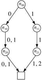
(a)	(b)

Figure 3: (a) A set of integer triples, (b) The corresponding MDD representation for the set shown in (a).

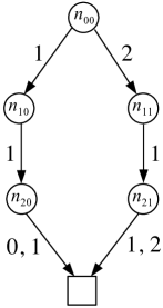
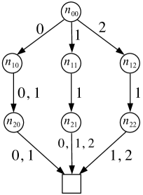
(a)	(b)

Figure 4: (a) Another multi-value decision diagram, (b) The result from merging the MDD in Fig .4(a) and the MDD in Fig. 3(b) by the union operation.

III-C Using Decision Diagrams in Reachability Analysis

A direct way to use the multi-value decision diagrams in the reachability analysis shown in Algorithm 1 is to replace the hash table for $stateTable$ with a decision diagram. First, let $\texttt{mdd\_create}(\vec{s}\hskip 2.0pt)$ be a function that takes an integer tuple and returns a multi-value decision diagram with a single path corresponding to $\vec{s}\hskip 2.0pt$. Then, the code in line 16 in Algorithm 1 can simply be replaced with the following line.

$stateTable=\texttt{union}(stateTable,~{}\texttt{mdd\_create}(\vec{s}\hskip 2.0pt^{\prime}));$

Directly using the decision diagrams as shown above is simple, and can be very efficient in memory usage. However, it is not very efficient in runtime. This is due to a large number of union calls as one is made for every new state $\vec{s}\hskip 2.0pt^{\prime}$. Since each union call can incur several operations on node creations and checks against the unique node table, a large number of union calls can lead to very high overhead when the number of reachable states is large.

To address this problem, multi-value decision trees are used as buffers for a set of states before adding them together into the decision diagram $stateTable$. The basic reason is that it is much more efficient to add a state into a decision tree. On the other hand, a decision tree generally requires more memory to store the same number of states than a decision diagram. In this method, a decision tree is used as a buffer. The search algorithm adds states into the decision tree first. When a sufficiently large number of states are added such that a preset memory threshold is exceeded, this decision tree is compressed to become a decision diagram, and consequently merged with the decision diagram pointed by $stateTable$ by function union. This is a common idea of trading a reasonable amount of memory for higher runtime efficiency.

Decision trees can be compressed into decision diagrams by function compress. This function takes a decision tree rooted at node $n$, and performs the following operations recursively.

1. Create a new node $n_{1}$.

2. For each edge ${(n,i,n^{\prime})}\in outgoing(n)$,

   1. $n^{\prime\prime}=\texttt{compress}(n^{\prime})$.

   2. Add edge ${(n_{1},i,n^{\prime\prime})}$ into $outgoing(n_{1})$.

3. Check if there exists an equivalent node to $n_{1}$ in the unique node table. If so, return the equivalent node; otherwise, return $n_{1}$.

Basically, function compress traverses a decision tree from the root node, and merges all equivalent nodes.

IV Experiments

TABLE I: Results from using different state representations on a set of asynchronous circuit designs and models of mutual exclusion examples. Time is in seconds, and memory is in MBs. $|S|$ is the numbers of states found at the end of reachability analysis. Entries filled with $900$ under Time and $2000$ under Mem indicate time-out and memory. Columns under “Base” show results using hash tables. Columns under “MDD” show results using MDDs, while those under “MDD-hybrid” show results using MDDs combined with decision trees as buffers.

	Base					MDD					MDD-Hybrid
Models	Time	Mem	$|S|$	SS	SSD	Time	Mem	$|S|$	SS	SSD	Time	Mem	$|S|$	SS	SSD
arbN5 (44)	4.1	53	227472	55481	4292	5.3	32	227472	42919	7109	4.3	45	227472	52900	5055
arbN7 (62)	292	2000	12582972	43092	6291	548	1109	13801104	25184	12445	448	1639	13801104	30806	8420
arbN9 (80)	113	2000	9052417	80110	4526	320	2000	15892574	49664	7946	277	2000	18241258	65853	9121
dmeN3 (33)	2.77	49	267999	96751	5469	4.3	21	267999	62325	12762	2.4	29	267999	111666	9241
dmeN4 (44)	199	1725	15692028	78854	9097	322	155	15692028	48733	101239	152	560	15692028	103237	28021
dmeN5 (55)	149	2000	12590803	84502	6295	900	1881	38823343	43137	20640	900	2000	66746007	74162	33373
fifoN8 (34)	119	653	3572036	30017	5470	900	924	3268850	3632	3538	102	689	3572036	35020	5184
fifoN10 (42)	292	2000	9481673	32471	4741	900	301	334460	372	1111	767	2000	13164188	17163	6582
mmu (55)	900	1528	8284885	9205	5422	900	757	5492496	6103	7256	900	1701	9057024	10063	5325
pipectrl (50)	168	2000	10485516	62414	5243	376	2000	14444726	38417	7222	398	2000	22082395	55483	11041
tagunit (48)	269	2000	3302662	12278	1651	900	1919	2546805	2830	1327	900	1752	2668985	2966	1523
anderson.6	141	2000	12013290	85201	6007	897	1724	18206917	20298	10561	348	1751	18206917	52319	10398
anderson.8	41	2000	9022879	220070	4511	187	2000	12222460	65361	6111	192	2000	16141525	84070	8071
at.4	102	1018	6597246	64679	6481	900	762	6159114	6843	8083	122	1624	6597246	54076	4062
at.5	154	2000	10489013	68110	5245	900	1028	3651887	4058	3552	900	1752	12581219	13979	7181
at.6	167	2000	10100451	60482	5050	900	1109	3651887	4058	3293	900	1752	11601860	12891	6622
at.7	361	2000	12583081	34856	6292	900	506	3651887	4058	7217	900	1751	17686712	19652	10101
bakery.8	214	2000	17042811	79639	8521	900	754	51820580	57578	68728	900	1751	76680860	85201	43793
driving_phils.3	1	13	436	436	34	1	14	436	436	31	1	14	436	436	31
driving_phils.4	204	2000	14039859	68823	7020	900	576	5217462	5797	9058	900	1752	28672594	31858	16366
driving_phils.5	78	2000	3599664	46150	1800	900	520	2268540	2521	4363	230	1750	3599663	15651	2057
fischer.3	52	409	2896705	55706	7082	900	329	2363979	2627	7185	66	897	2896705	43889	3229
fischer.4	25	342	1272254	50890	3720	471	461	1272254	2701	2760	47	1135	1272254	27069	1121
fischer.5	340	2000	10780321	31707	5390	900	552	2505498	2784	4539	900	1752	5199544	5777	2968
fischer.6	299	2000	8237316	27550	4119	900	533	2022330	2247	3794	900	1751	3811183	4235	2177
fischer.7	365	2000	10633261	29132	5317	900	497	2717506	3019	5468	900	1752	7996790	8885	4564
lamport.5	10	135	1066799	106680	7902	19	51	1066799	56147	20918	10.2	110	1066799	104588	9698
lamport.6	1	11	519	519	47	1	14	519	519	37	1	12	519	519	43
lamport.7	252	2000	18075514	71728	9038	900	310	33954095	37727	109529	497	1751	38717845	77903	22112
lamport.8	1	11	50	50	5	1	11	50	50	5	1	11	50	50	5
mcs.5	127	2000	12041513	94815	6021	900	1801	15106694	16785	8388	363	2000	23015234	63403	11508
peterson.4	11	147	1119559	101778	7616	21	68	1119559	53312	16464	11	161	1119559	101778	6954
peterson.5	109	2000	12583035	115441	6292	727	2000	23998663	33011	11999	517	2000	42200403	81626	21100
peterson.6	88	2000	11110639	126257	5555	486	2000	13820828	28438	6910	309	2000	23897297	77338	11949
peterson.7	222	2000	15975060	71960	7988	900	692	11957462	13286	17280	900	1752	64062366	71180	36565
phils.6*	2.5	159	241660	96664	1520	14	141	241660	17261	1714	4	617	241660	60415	392
phils.7	44	2000	6927036	157433	3464	900	1715	10253596	11393	5979	261	2000	10486177	40177	5243
phils.8	7.2	437	914351	126993	2092	144	373	914351	6350	2451	13	1707	914351	70335	536
szymanski.4	20.4	282	2313863	113425	8205	46	78	2313863	50301	29665	21	204	2313863	110184	11342
szymanski.5	155	2000	15908655	102636	7954	900	527	48526313	53918	92080	867	1751	79514858	91713	45411
Average				69875	5220				22155	16269				49263	10712

The multi-value decision trees and diagrams described in this paper are implemented in a package, and integrated into an asynchronous system verification tool $Platu$, an explicit model checker implemented in Java. Experiments have been been performed on a number of examples. These examples include asynchronous circuit designs from previously published papers [13, 7, 20, 21, 15]. Other examples are selected from the BEEM benchmark suite for explicit model checking [16]. This benchmark includes a large number of models of communication protocols, mutual exclusion algorithms, etc. All the examples used in the experiments have medium or high complexity to show the difference in using the hash tables and the decision diagrams.

In the experiments, all examples are ran by using the same depth-first search algorithm but with three different ways for storing reachable states: hash table, multi-value decision diagram, and multi-value decision diagram with a decision tree as buffer to reduce runtime overhead. To have somewhat fair comparison, the model checker SPIN [12] is not used in the experiments since SPIN is implemented in C while Platu is implemented in Java. It is well known that the Java applications generally have serious memory overhead. Instead, the state compression technique implemented in SPIN is also implemented in Platu, and used as the base of state representation for all three methods representing reachable sets of states.

Among all the examples, some have very large state space, and it can take enormous amount of time to find all reachable states. The main purpose of using the decision diagrams for storing reachable states is to allow much larger number of states to be explored in a reasonable amount of time. Hash tables can be accessed very efficiently, but usually exhaust memory also very quickly. Therefore, for examples with small state space, hash tables are a better option. On the other hand, for large examples, the decision diagrams would allow either the whole state space or a much larger portion of it to be stored with some extra runtime. This allows larger examples to be handled, or improves verification coverage by exploring significantly more states. In all experiments, upper bounds on time and memory are set to $900$ seconds and $2$ GB. The results collected include the actual runtime, memory usage, and the total number of reachable states found at termination of the search algorithm. In cases of time-out or memory-out, the number of reachable states is recorded. All experiments are performed on a iMac desktop with a Intel Quad-core processor. Only a single thread is used for all experiments.

The results are shown in Table I. The first column Column shows the different models. The numbers enclosed in parenthesis for the first few examples indicate the number of state variables. Since these examples are asynchronous circuits, the type of their state variables is boolean. The following examples are the models of mutual exclusion algorithms from the BEEM benchmarks [16]. The remaining columns are divided into three groups, one for results from using each different state representation. Columns under “Base” show results with the hash table is used. Columns “MDD” show the results with the MDD alone used. Finally, the columns under “MDD-Hybrid” show the results with MDD used where a decision tree is used to speed up the search. Among the five columns in each group, “Time” and “Mem” show the total runtime and the peak memory used during the search. Note that the memory numbers include those used for storing reachable states and other necessary data structures for the search such as stacks. Column “$|S|$” shows the total number of states found at the termination of the search. Note that this number shows all reachable states of an example if the run does not time out ($<900$ second) and does not exhaust the allocated memory ($<2000$ MB).

The first conclusion that can be drawn from the table is that the search using a hash table is the fastest for almost all examples. For examples with low complexity such as at.4 and fischer.3. However, using a hash table also causes the search to exhaust 2 GB for large number of examples as shown by the cells in the table under “Mem” filled with 2000. On the other hand, from the columns under “MDD”, the search with MDD used is significantly slower, and it times out for most examples. At the same time, using MDD allows more states to be searched with less memory. Take dmeN5 as an example. using MDD causes the search to time out, but over two times more states are found with slightly less memory than $2$ GB used. The same conclusion is also observed for anderson.8, lamport.7, and so on. For some other examples, the search with the MDD finds less number of states due to the overhead from converting states into the MDDs as explained before. Finally, from the columns under “MDD-Hybrid”, the search in this mode finds much more states for almost every example within both limits of time and memory. This shows the effectiveness of using decision trees as buffer for the MDD representation.

To better compare these three representations, two more values are computed from the results for each example: search speed (SS) and state space density (SSD). The numbers in the column under SS show the numbers of states found per second. This is a rough measure of how fast the search runs. The numbers in the column under SSD show the numbers of states per MB of memory. This is a rough measure of the efficiency of different representations for storing states. For both measures, it is better and more efficient if the numbers are larger. The averages of these two measurements are shown in the last row for every group. From the average numbers, it can be seen alternatively that using the hash tables leads to the highest search speed but the least memory efficiency. Using MDD alone leads to the highest memory efficiency, but it is the slowest to use. The MDD with the decision tree buffering achieves good balance between runtime and memory as it is slight slower than using hash tables, and slightly less memory efficient than using the MDDs alone. This good balance allows the search to find much more states for many examples. Take szymamski.5 as an example, the search exceeds the memory limits by finding a little over 15 million states when the hash table is used, while the search runs out of time after finding about 2 times more states with only 527 MB memory used when the MDDs alone are used. However, the MDDs with buffering allow all reachable states to be found under both time and memory limits.

From the experiments, for examples that take long time to run for the search using hash tables, using the MDDs would lead to less number of states to be found as it is more expensive to use the MDDs even with faster buffering techniques. On the other hand, for examples that have large state space, the MDDs are much more efficient. Furthermore, buffering seems a very promising approach for handling larger designs. Since the MDDs implemented in Platu are not intensively optimized, there might be more potential for making them even more efficient. Meanwhile, it would be interesting to investigate if using the existing BDD packages such as CUDD [18] could bring more efficiency as they commonly support variable recording, which is well known critical for efficiency and compactness of BDD representations.

One last point to note is that in the work described in this paper, these different approaches are experimented to find out how states can be stored efficiently. The depth-first search algorithm itself remains the same. This indicates that partial order reduction can be naturally integrated with the MDDs to allow much larger designs to be handled. However, partial order reduction is not used in this paper.

V Conclusion

This paper shows how the multi-value decision diagrams are used to store reachable states efficiently and compactly, which allows larger designs to be verified, or more states to be explored thus improving the verification coverage. By using the decision trees as a buffering technique, the overhead of using the multi-value decision diagrams is significantly reduced. In the future, it is interesting to find out how the binary decision diagrams compare against the multi-value decision diagrams in the same context. Moreover, combining the decision diagrams and partial order reduction will also be investigated.

References

- [1] J. Ahrens. A compositional approach to asynchronous design verification with automated state space reduction. Master’s thesis, Univ. of South Florida, 2007.
- [2] G. Brat, K. Havelund, S. Park, and W. V. Java. Pathfinder c a second generation of a java model-checker. In Workshop on Advances in Verification, 2000.
- [3] R. E. Bryant. Symbolic Boolean manipulation with ordered binary-decision diagrams. ACM Computing Surveys, 24(3):293–318, 1992.
- [4] J. Burch, E. Clarke, D. Long, K. McMillan, and D. Dill. Symbolic model checking for sequential circuit verification. IEEE Transactions on Computer-Aided Design of Integrated Circuits and Systems, 13(4):401–424, 1994.
- [5] C.Baier and J.-P.Katoen. Principles of Model Checking. MIT Press, 2008.
- [6] G. Ciardo, G. L ttgen, and R. Siminiceanu. Saturation: an efficient iteration strategy for symbolic state space generation. In PROC. TOOLS AND ALGORITHMS FOR THE CONSTRUCTION AND ANALYSIS OF SYSTEMS (TACAS), LNCS 2031, pages 328–342. Springer-Verlag, 2001.
- [7] D. Dill. Trace Theory for Automatic Hierarchical Verification of Speed Independent Circuits. PhD thesis, Carnegie Mellon University, 1988.
- [8] E.M.Clarke, O.Grumberg, and D.Peled. Model Checking. MIT Press, 2000.
- [9] G.J.Holzmann and D.Peled. An improvement in formal verification. In roc. Seventh FORTE Conf. Formal Description Techniques, 1994.
- [10] P. Godefroid. Partial-Order Methods for the Verification of Concurrent Systems: An approach to the State-Explosion Problem. PhD thesis, University of Liege, 1995.
- [11] G. Holzmann. The SPIN Model Checker: Primer and Reference Manual. Addison-Wesley Professional, Cambridge, Mass., 2003.
- [12] G. J. Holzmann. The model checker SPIN. Software Engineering, 23(5):279–295, 1997.
- [13] A. J. Martin. Self-timed fifo: An exercise in compiling programs into vlsi circuits. Technical Report 1986.5211-tr-86, California Institute of Technology, 1986.
- [14] T. Murata. Petri nets: Properties, analysis, and applications. In Proceedings of the IEEE 77(4), pages 541–580, 1989.
- [15] C. J. Myers. Computer-Aided Synthesis and Verification of Gate-Level Timed Circuits. PhD thesis, Stanford University, 1995.
- [16] R. Pelánek. Beem: Benchmarks for explicit model checkers. In Proc. of SPIN Workshop, volume 4595 of LNCS, pages 263–267. Springer, 2007.
- [17] R.A.Thacker, K.R.Jones, C.J.Myers, and H. Zheng. Automatic abstraction for verification of cyber-physical systems. In 1st International Conference on Cyber-Physical Systems, 2010.
- [18] F. Somenzi. Cudd: Cu decision diagram package.
- [19] A. Srinivasan, T. Ham, S. Malik, and R. Brayton. Algorithms for discrete function manipulation. In Proceedings of Computer-Aided Design, 1990. ICCAD-90. Digest of Technical Papers., 1990 IEEE International Conference on, pages 92–95, Nov 1990.
- [20] K. Stevens, R. Ginosar, and S. Rotem. Relative timing. In Proc. International Symposium on Advanced Research in Asynchronous Circuits and Systems, pages 208–218, 1999.
- [21] T. Yoneda and T. Yoshikawa. Using partial orders for trace theoretic verification of asynchronous circuits. In Proc. of Second International Symposium on Advanced Research in Asynchronous Circuits and Systems, pages 152–163, 1996.