, , and m1Department of Mathematical Sciences, Indiana University - Purdue University Indianapolis, IN 46202, USA. k1Department of Mathematical Sciences, New Jersey Institute of Technology, NJ 07102, USA. k2Department of Statistics, Purdue University, IN 47907, USA.

Working Paper Version

On Deep Instrumental Variables Estimate

Abstract

The endogeneity issue is fundamentally important as many empirical applications may suffer from the omission of explanatory variables, measurement error, or simultaneous causality. Recently, Hartford et al., (2017) propose a “Deep Instrumental Variable (IV)” framework based on deep neural networks to address endogeneity, demonstrating superior performances than existing approaches. The aim of this paper is to theoretically understand the empirical success of the Deep IV. Specifically, we consider a two-stage estimator using deep neural networks in the linear instrumental variables model. By imposing a latent structural assumption on the reduced form equation between endogenous variables and instrumental variables, the first-stage estimator can automatically capture this latent structure and converge to the optimal instruments at the minimax optimal rate, which is free of the dimension of instrumental variables and thus mitigates the curse of dimensionality. Additionally, in comparison with classical methods, due to the faster convergence rate of the first-stage estimator, the second-stage estimator has a smaller (second order) estimation error and requires a weaker condition on the smoothness of the optimal instruments. Given that the depth and width of the employed deep neural network are well chosen, we further show that the second-stage estimator achieves the semiparametric efficiency bound. Simulation studies on synthetic data and application to automobile market data confirm our theory.

Keywords: Deep Learning, Efficiency Bound, Endogeneity, Instrumental Variables, Semiparametric Model.

1 Introduction

Endogeneity is a common issue in empirical studies and naturally arises from simultaneous causality, omitted variables, or measurement errors (Terza et al.,, 2008; Attfield,, 1985; Yun,, 1996; Melitz,, 2003). In the presence of endogeneity, the ordinary least squares (OLS) estimator is known to be inconsistent. One signature tool in addressing the endogeneity issue is to use the so-called two-stage least squares (2SLS) procedure by introducing instrumental variables (IV), as widely used in the literature (Angrist and Keueger,, 1991; Staiger and Stock,, 1997; Parker and Van Praag,, 2006; Lin and Liscow,, 2012). However, the 2SLS estimator is generally inefficient if the reduced form equation between instrumental variables and endogenous variables is not linear. Therefore, as pointed out by Amemiya, (1974) and Newey, (1990), to obtain an efficient estimator, one needs to find the optimal IVs, which involves estimating a set of unknown functions.

Various non/semiparametric approaches have been proposed to estimate the optimal IVs with guaranteed efficiency (Amemiya,, 1974; Newey,, 1990; Newey et al.,, 1999; Newey and Powell,, 2003); nonetheless, they could suffer from the curse of dimensionality in the presence of many IVs. To overcome this difficulty, Belloni et al., (2012) assume that the optimal IVs can be approximated by a series of basis and propose a lasso-like algorithm to estimate the optimal instruments. Following Belloni et al., (2012), Fan and Zhong, (2018) impose an additive structure assumption on the optimal IVs, which yields dimension-free results, whereas their estimator could be inefficient when the additive structure fails to hold. This motivates Hartford et al., (2017) to propose a very flexible deep learning framework, named as Deep IV, under which impressive empirical performances are demonstrated even when IVs are high-dimensional and the optimal IVs are of complex structures. Based on the same framework, Bennett et al., (2019) further propose a Deep Generalized Method of Moments (Deep GMM) for the IV analysis, while Farrell et al., (2019) use a two-stage estimator based on neural networks to conduct inferences on the treatment effect. As discussed in Hartford et al., (2017), in comparison with Deep IV, the classical series or kernel estimation (e.g., Newey and Powell,, 2003; Blundell et al.,, 2007; Chen and Pouzo,, 2012; Belloni et al.,, 2012) is computationally intractable in high-dimensional feature spaces. However, theoretical understandings on the benefits of the use of deep neural networks in the IV analysis are still missing.

The present work aims to theoretically explain the empirical success of the Deep IV framework. For simplicity of presentation, we mainly consider the linear regression model with endogenous predictors and observable IVs. In the first stage, using the IVs as the regressors and endogenous variables as the responses, the optimal IVs are estimated by a fully connected rectifier linear unit (ReLU) deep neural network (DNN). By imposing a general compositional structure assumption on the optimal IVs, we derive the convergence rate for the proposed neural network estimator, which is free of the dimension of IVs, as either depth, width, or both diverge. In particular, the derived rate is minimax optimal as long as the product of depth and width for the neural network is greater than the number of IVs and is a polynomial order of the sample size. In practice, the implementation of DNN does not explicitly rely on the imposed structure assumption, i.e., latent compositional structure, unlike additive or linear regression. As a side remark, the choices of depth and width have different impacts on the numerical optimization in learning the neural network. Specifically, to obtain the optimal convergence rate, a very deep network is more “economical” in terms of the number of parameters to be learned; on the other hand it faces the challenge of the vanishing gradient issue in comparison with shallow neural networks.

In the second stage, we perform the least squares estimation for the linear coefficients based on the estimated optimal IVs in the first stage. If the product of depth, width, and IV dimension is of a polynomial order of sample size, the estimator is proven to be asymptotically normal and achieve the semiparametric efficiency bound (Bickel et al.,, 1993) as either depth, width, or both diverge. Moreover, by taking advantage of the faster convergent neural network estimate, the second-stage estimate not only has a smaller (second order) estimation error (in the sense of Cheng and Kosorok, (2008) to be explained later) but also requires a weaker condition on the smoothness of the optimal IVs when compared with classical methods. Specifically, using polynomial spline basis, the series approach in Belloni et al., (2012) requires that the smoothness degree of the optimal IVs should be greater than half of the IV dimension. In contrast, our results hold as long as the intrinsic smoothness degree of the optimal IVs is greater than half of their intrinsic dimension, which will be proven to be weaker. To be more concrete, we present a scenario where our estimator outperforms some widely used estimators in the literature; see Example 4.

Several extensions can be made based on the above theoretical results. To be more specific, we propose a sample-split estimator to remove the requirement on the intrinsic smoothness and intrinsic dimension of the optimal IVs. A specification testing procedure is also proposed to test the validity of the instrumental variables based on deep neural network. Finally, we consider an extended model containing both endogenous and exogenous variables.

Recently, a number of researchers study deep neural networks from nonparametric perspective. To name a few, Bauer and Kohler, (2019) and Schmidt-Hieber, (2019) use sparse neural network in the nonparametric regression setting, while Kim et al., (2018) study the problem of classification based on sparse network. Recently, Kohler and Langer, (2019) extend the result in Bauer and Kohler, (2019) to very deep (diverging depth) fully connected neural network with fixed width. Our IV estimator is a fully connected neural network with either depth, width, or both being diverging. This more flexible network structure, which covers the network architecture in Kohler and Langer, (2019), avoids the selection of sparsity parameter in practice and does not need to impose a truncation parameter to bound the neural network estimation, in contrast with Bauer and Kohler, (2019); Schmidt-Hieber, (2019); Kohler and Langer, (2019). Our theoretical results are derived by extending the recent neural network approximation theory in Lu et al., (2020) from Sobolev space to Hölder space.

This paper is organized as follows. Section 2 reviews mathematical formulation of linear IV model. Section 3 describes the Deep IV estimation procedure. Section 4 provides the asymptotic results of the proposed estimator and its advantages over the existing approaches. Section 5 provides some additional inferential procedures based on deep neural network. Section 6 compares the finite-sample performance of our estimator and some completing approaches through a simulation study. Section 7 applies the proposed procedure to a real-world data set to study the connection between automobile sales and price. All the mathematical proofs are deferred to the Appendix.

2 Linear Instrumental Variable Model

Consider i.i.d. observations $\{Y_{i},\mathbf{X}_{i}\}_{i=1}^{n}$ generated from the following linear regression model:

$$Y=\beta_{0}^{\top}\mathbf{X}+\epsilon,$$ (2.1)

where $Y\in\mathbb{R}$ is the response variable, $\mathbf{X}=(X_{1},\ldots,X_{q})^{\top}\in\mathbb{R}^{q}$ is the vector of explanatory variables, $\epsilon$ is the random noise, and $\beta_{0}\in\mathbb{R}^{q}$ is the vector of unknown coefficients. The explanatory variables $X_{1},\ldots,X_{q}$ are assumed to be endogenous in the sense that

$$\textrm{Cov}(\epsilon,X_{s})\neq 0,\quad\textrm{ for all }s=1,\ldots,q.$$

In order to consistently estimate $\beta_{0}$, one set of instrumental variables $\mathbf{Z}=(Z_{1},\ldots,Z_{d})^{\top}\in\mathbb{R}^{d}$ with i.i.d. observations $\{\mathbf{Z}_{i}\}_{i=1}^{n}$ is introduced as follows (e.g., see Wooldridge,, 2008):

$$\mathbb{E}(\epsilon|Z_{j})=0,\quad\textrm{ for all }j=1,\ldots,d.$$ (2.2)

In view of (2.1) and (2.2), one set of unconditional moment equations to identify $\beta_{0}$ is

$$\mathbb{E}[(Y-\beta_{0}^{\top}\mathbf{X})\mathbf{h}(\mathbf{Z})]=0,\quad\textrm{ for all $q$-dimensional vector-valued measurable function }\mathbf{h}.$$ (2.3)

Define a collection of optimal IVs:

$$\mathbf{h}_{\textrm{opt}}(\mathbf{z})\mathrel{\mathop{\mathchar 58\relax}}=(f_{0,1}(\mathbf{z}),\ldots,f_{0,q}(\mathbf{z}))^{\top}\;\;\mbox{with}\;\;f_{0,s}(\mathbf{z})\mathrel{\mathop{\mathchar 58\relax}}=\mathbb{E}(X_{s}|\mathbf{Z}=\mathbf{z}).$$

By setting $\mathbf{h}(\mathbf{z})=\mathbf{h}_{\textrm{opt}}(\mathbf{z})$ in (2.3), the corresponding method of moments estimator solved through (2.4) can be proven to be semiparametric efficient (see Amemiya,, 1974 and Newey,, 1990):

$$\frac{1}{n}\sum_{i=1}^{n}(Y_{i}-\beta^{\top}\mathbf{X}_{i})\widehat{\mathbf{h}}_{\textrm{opt}}(\mathbf{Z}_{i})=0,$$ (2.4)

where $\widehat{\mathbf{h}}_{\textrm{opt}}$ is an estimate for ${\mathbf{h}}_{\textrm{opt}}$.

This above idea has been exhaustively studied based on various forms of $\widehat{\mathbf{h}}_{\textrm{opt}}$. For example, Newey, (1990) uses both k-nearest-neighbors and series approximation methods to estimate ${\mathbf{h}}_{\textrm{opt}}$. As pointed out by Cheng and Kosorok, (2008) in a general semiparametric setting, the convergence rate of $\widehat{\mathbf{h}}_{\textrm{opt}}$ to ${\mathbf{h}}_{\textrm{opt}}$ plays an important role in estimating $\beta_{0}$: the second order error in estimating $\beta_{0}$ based on (2.4) is smaller when $\widehat{\mathbf{h}}_{\textrm{opt}}$ converges at a faster rate. Moreover, in order to ensure semiparametric efficiency for estimating $\beta$, $\widehat{\mathbf{h}}_{\textrm{opt}}$ is required to converge to $\mathbf{h}_{\textrm{opt}}$ at a sufficiently fast rate. However, when the dimension of $\mathbf{Z}$ is large, the convergence rate is often slow due to the curse of dimensionality. To address this issue, Belloni et al., (2012) impose a sparsity assumption that ${\mathbf{h}}_{\textrm{opt}}$ can be approximated by a functional series and then estimated by a lasso-type series estimator. Following Belloni et al., (2012), Fan and Zhong, (2018) assume that each element of $\mathbf{h}_{\textrm{opt}}$, namely $f_{0,s}$, follows an additive model of $Z_{1},\ldots,Z_{d}$. However, if $\mathbf{h}(\mathbf{z})$ has interaction terms, this method could lead to an inefficient estimator due to model misspecification. Recently, Hartford et al., (2017) consider the pure nonparametric regression $Y=g(\mathbf{X})+\epsilon$ with $\mathbf{X}$ being endogenous. They propose the Deep IV procedure based on two deep nerual networks to estimate the underlying regression function. A followup work of Deep IV is Deep GMM for instrumental variables analysis by Bennett et al., (2019). Both Deep IV and Deep GMM demonstrate very impressive empirical performances but with very limited theoretical investigation. The aim of our work is to understand the theoretical benefits of the use of deep neural networks in instrumental variables analysis.

Notation: Let $\|\mathbf{v}\|_{2}^{2}=\mathbf{v}^{\top}\mathbf{v}$ denote the Euclidean norm of the vector $\mathbf{v}$. Let $\xrightarrow[\text{}]{\text{$\mathbb{L}$}}$ and $\xrightarrow[\text{}]{\text{$\mathbb{P}$}}$ denote the convergence in distribution and convergence in probability, respectively. For two sequence $a_{n}$ and $b_{n}$, we say $a_{n}\asymp b_{n}$ if $c^{-1}a_{n}\leq b_{n}\leq ca_{n}$ for some constant $c>1$ and all sufficiently large $n$. For each observation, let $X_{i1},\ldots,X_{iq}$ and $Z_{i1},\ldots,Z_{id}$ be the elements of $\mathbf{X}_{i}$ and $\mathbf{Z}_{i}$. For any $f\mathrel{\mathop{\mathchar 58\relax}}\mathbb{R}^{d}\to\mathbb{R}$, define the $L^{2}$-norm $\|f\|^{2}=\mathbb{E}(f^{2}(\mathbf{Z}))$ and its empirical counter part $\|f\|_{n}^{2}=n^{-1}\sum_{i=1}^{n}f^{2}(\mathbf{Z}_{i})$. For $a>0$, let $\left\lfloor a\right\rfloor$ denote the largest integer strictly less than $a$ and ${\lceil a\rceil}=\left\lfloor a\right\rfloor+1$. We say $(L,W)\to\infty$, if ether $L$, $W$ or both diverge.

3 Deep Instrumental Variables Estimation

In this section, we first review the setup for fully connected neural networks. Let $\sigma$ denote the ReLU activation function, i.e., $\sigma(x)\mathrel{\mathop{\mathchar 58\relax}}=(x)_{+}$ for $x\in\mathbb{R}$. For any $r$-dimensional real vectors $\mathbf{v}=(v_{1},\ldots,v_{r})^{T}$ and $\mathbf{a}=(a_{1},\ldots,a_{r})^{T}$, define the shift activation function $\bm{\sigma}_{\mathbf{v}}(\mathbf{a})=(\sigma(a_{1}-v_{1}),\ldots,\sigma(a_{r}-v_{r}))^{T}$. Moreover, a vector-valued function $\mathbf{f}\mathrel{\mathop{\mathchar 58\relax}}\mathbb{R}^{d}\to\mathbb{R}^{q}$ is a fully connected deep neural network with depth $L$ and width $W$, if it has the following expression:

$$\mathbf{f}(\mathbf{z})=\mathbf{v}_{L+1}+\mathbf{A}_{L+1}\bm{\sigma}_{\mathbf{v}_{L}}\circ\mathbf{A}_{L}\bm{\sigma}_{\mathbf{v}_{L-1}}\circ\ldots\circ\mathbf{A}_{2}\bm{\sigma}_{\mathbf{v}_{1}}\circ\mathbf{A}_{1}\mathbf{z},\quad\quad\textrm{ for }\mathbf{z}\in\mathbb{R}^{d},$$ (3.1)

where $\mathbf{v}_{L+1}\in\mathbb{R}^{q}$ and $\mathbf{v}_{l}\in\mathbb{R}^{W}$ for $l=1,\ldots,L$ are the shift vectors, $\mathbf{A}_{1}\in\mathbb{R}^{W\times d},\mathbf{A}_{L+1}\in\mathbb{R}^{q\times W}$ and $\mathbf{A}_{l}\in\mathbb{R}^{W\times W}$ for $l=2,\ldots,L$ are the weight matrices. Finally, we denote $\mathcal{F}_{d,q}(L,W)$ as the collection of fully connected deep neural networks with depth $L$, width $W$, $d$-dimensional input and $q$-dimensional output.

We propose a two-stage estimation procedure based on the fully connected neural network. The first stage is to construct a DNN estimate as $\widehat{\mathbf{h}}_{\textrm{opt}}$:

$$\widehat{\mathbf{f}}\mathrel{\mathop{\mathchar 58\relax}}=\operatorname*{argmin}_{\begin{subarray}{c}\mathbf{f}\in\mathcal{F}_{d,q}(L,W)\end{subarray}}\frac{1}{n}\sum_{i=1}^{n}\|\mathbf{X}_{i}-\mathbf{f}(\mathbf{Z}_{i})\|_{2}^{2},$$ (3.2)

where the elements of $\widehat{\mathbf{f}}$ can be written as $(\widehat{f}_{1},\ldots,\widehat{f}_{q})^{\top}$. Correspondingly, we define $\widehat{\mathbf{X}}_{i}\mathrel{\mathop{\mathchar 58\relax}}=\widehat{\mathbf{f}}(\mathbf{Z}_{i})=(\widehat{f}_{1}(\mathbf{Z}_{i}),\ldots,\widehat{f}_{q}(\mathbf{Z}_{i}))^{\top}\in\mathbb{R}^{q}$ for $i=1,\ldots,n$. As will be shown in Theorem 1, the DNN estimation procedure is able to capture the intrinsic structure of ${\mathbf{h}}_{\textrm{opt}}$ without explicitly using the prior information of its compositional structure (to be specified later). The second stage is to construct an estimator of $\beta_{0}$ in an OLS manner:

$$\widehat{\beta}=\bigg{(}\frac{1}{n}\sum_{i=1}^{n}\widehat{\mathbf{X}}_{i}\mathbf{X}_{i}^{\top}\bigg{)}^{-1}\frac{1}{n}\sum_{i=1}^{n}\widehat{\mathbf{X}}_{i}Y_{i}.$$ (3.3)

Intuitively, if the DNN estimators $\widehat{f}_{1},\ldots,\widehat{f}_{q}$ are close to the ground truth $f_{0,1},\ldots,f_{0,q}$ enough, the second-stage estimator will be also close to the “oracle” estimator obtained by using the ground truth in (3.3), which is known to achieve semiparametric efficiency.

It is worth mentioning that the optimization problem in (3.2) is unconstrained, and it is usually solved by the Stochastic Gradient Descent (SGD) algorithm or its variants. However, the neural network estimators proposed by Bauer and Kohler, (2019) and Kohler and Langer, (2019) are truncated by a threshold parameter, while Schmidt-Hieber, (2019) needs to solve a constrained optimization problem requiring the estimator is bounded by some predetermined constant. Therefore, our estimator is practically convenient and avoids the issue of choosing all inds of hyper-parameters. Furthermore, the neural networks considered in Bauer and Kohler, (2019) and Schmidt-Hieber, (2019) are both sparse; namely, some of the weights should be zero. In practice, how to determine the sparsity is difficult. Recently, Kohler and Langer, (2019) extend their earlier work Bauer and Kohler, (2019) to fully connected networks, but require $W$ to be fixed. Rather, our estimator in (3.2) allows either $L$, $W$, or both to diverge, which is more practically flexible.

4 Asymptotic Theory

In this section, we develop rate of convergence for $\widehat{\mathbf{f}}$ and asymptotic distribution for $\widehat{\beta}$.

4.1 Rate of Convergence

We begin with the definitions of Hölder smooth function and a class of multivariate functions with a compositional structure.

Definition D1.

A function $g\mathrel{\mathop{\mathchar 58\relax}}\mathbb{R}^{d}\to\mathbb{R}$ is said to be $(p,C)$-Hölder smooth for some positive constants $p$ and $C$, if for every $\bm{\gamma}=(\gamma_{1},\ldots,\gamma_{d})\in\mathbb{N}^{d}$ the following two conditions hold:

$$\sup_{\mathbf{z}\in\mathbb{R}^{d}}\bigg{|}\frac{\partial^{|\bm{\gamma}|}g}{\partial z_{1}^{\gamma_{1}}\ldots\partial z_{1}^{\gamma_{d}}}(\mathbf{z})\bigg{|}\leq C,\quad\textrm{ for all }|\bm{\gamma}|\leq\left\lfloor p\right\rfloor,$$

and

$$\bigg{|}\frac{\partial^{|\bm{\gamma}|}g}{\partial z_{1}^{\gamma_{1}}\ldots\partial z_{1}^{\gamma_{d}}}(\mathbf{z})-\frac{\partial^{|\bm{\gamma}|}g}{\partial z_{1}^{\gamma_{1}}\ldots\partial z_{1}^{\gamma_{d}}}(\widetilde{\mathbf{z}})\bigg{|}\leq C\|\mathbf{z}-\widetilde{\mathbf{z}}\|_{2}^{p-\left\lfloor p\right\rfloor},\quad\textrm{ for all }|\bm{\gamma}|=\left\lfloor p\right\rfloor\textrm{ and }\mathbf{z},\widetilde{\mathbf{z}}\in\mathbb{R}^{d}.$$

Here $|\bm{\gamma}|=\sum_{i=1}^{d}\gamma_{d}$. For convenience, we say $g$ is $(\infty,C)$-Hölder smooth convenience if $g$ is $(p,C)$-Hölder smooth for all $p>0$.

Definition D2.

A function $f\mathrel{\mathop{\mathchar 58\relax}}\mathbb{R}^{d}\to\mathbb{R}$ is said to have a compositional structure with parameters $(L_{*},\mathbf{d},\mathbf{t},\mathbf{p},\mathbf{a},\mathbf{b},C)$ for $L_{*}\in\mathbb{Z}_{+}$, $\mathbf{d}=(d_{0},\ldots,d_{L_{*}+1})\in\mathbb{Z}_{+}^{L_{*}+2}$ with $d_{0}=d,d_{L_{*}+1}=1$, $\mathbf{t}=(t_{0},\ldots,t_{L_{*}})\in\mathbb{Z}_{+}^{L_{*}+1}$, $\mathbf{p}=(p_{0},\ldots,p_{L_{*}})\in\mathbb{R}_{+}^{L_{*}+1}$, $\mathbf{a}=(a_{0},\ldots,a_{L_{*}+1}),\mathbf{b}=(b_{0},\ldots,b_{L_{*}+1})\in\mathbb{R}^{L_{*}+2}$ and $C\in\mathbb{R}_{+}$, if

$$f(\mathbf{z})=\mathbf{g}_{L_{*}}\circ\ldots\circ\mathbf{g}_{1}\circ\mathbf{g}_{0}(\mathbf{z}),\quad\quad\textrm{ for all }\mathbf{z}\in[a_{0},b_{0}]^{d}$$

where $\mathbf{g}_{i}=(g_{i,1},\ldots,g_{i,d_{i+1}})^{\top}\mathrel{\mathop{\mathchar 58\relax}}[a_{i},b_{i}]^{d_{i}}\to[a_{i+1},b_{i+1}]^{d_{i+1}}$ for some $|a_{i}|,|b_{i}|\leq C$ and the functions $g_{i,j}\mathrel{\mathop{\mathchar 58\relax}}[a_{i},b_{i}]^{t_{i}}\to[a_{i+1},b_{i+1}]$ are $(p_{i},C)$-Hölder smooth only relying on $t_{i}$ variables. We denote $\mathcal{C}\mathcal{S}(L_{*},\mathbf{d},\mathbf{t},\mathbf{p},\mathbf{a},\mathbf{b},C)$ as the class of functions defined above

Definition D1 characterizes the smoothness of the regression function which is commonly used in the nonparametric literature (see Györfi et al.,, 2006; Huang,, 2003). Definition D2 requires that the function $f$ is a composition of $L_{*}+1$ layers with each layer being a vector-valued multivariate function which demonstrates a local connectivity structure. Such a compositional structure, also adopted by Bauer and Kohler, (2019), Schmidt-Hieber, (2019) and Kohler and Langer, (2019), is naturally motivated from the structure of the neural network. The functions $g_{i,j}$’s can be viewed as hidden features of the target function $f$, which makes up more complex features $g_{i+1,j}$’s in the next layer. One essence of deep neural network is to learn these hidden features from the data (Zeiler and Fergus,, 2014).

It is worthwhile to discuss the connection between Definitions D1 and D2. For this purpose, we define the following two important quantities:

$$p^{*}=p_{i^{*}}^{*}\quad\textrm{ and }\quad t^{*}=t_{i^{*}},$$

where $p_{i}^{*}=p_{i}\prod_{s=i+1}^{L_{*}}(p_{s}\wedge 1)$ for $i=0,\ldots,L_{*}$, and $i^{*}=\operatorname*{argmin}_{0\leq i\leq L_{*}}p_{i}^{*}/t_{i}$. We will adopt the convention $\prod_{s=L_{*}+1}^{L_{*}}(p_{s}\wedge 1)=1$ for convenience. Similar to Bauer and Kohler, (2019) and Schmidt-Hieber, (2019), $p^{*}$ and $t^{*}$ can be interpreted as the intrinsic smoothness and intrinsic dimension of a function satisfying Definition D2, and $t^{*}$ tends to be smaller than the input dimension $d$ in several important models, as seen from examples below.

It is not difficult to verify that a $(p,C)$-Hölder smooth function has a trivial compositional structure with $L_{*}=0$. On the other hand, the following lemma indicates that the functions with a compositional structure are also Hölder smooth.

Lemma 1.

1. Suppose $g_{1}\mathrel{\mathop{\mathchar 58\relax}}\mathbb{R}^{q}\to\mathbb{R}$ is $(p_{1},C)$-Hölder smooth and $\mathbf{g}_{2}=(g_{21},\ldots,g_{2q})\mathrel{\mathop{\mathchar 58\relax}}\mathbb{R}^{d}\to\mathbb{R}^{q}$ with $g_{2i}$’s are all $(p_{2},C)$-Hölder smooth, then degree of Hölder smoothness of $g_{1}\circ\mathbf{g}_{2}$ is $\min\{p_{1}p_{2},p_{1},p_{2}\}$.

2. If $f\in\mathcal{C}\mathcal{S}(L_{*},\mathbf{d},\mathbf{t},\mathbf{p},\mathbf{a},\mathbf{b},C)$, then the degree of Hölder smoothness of $f$ is $p_{H}\leq p^{*}$.

The conclusion (i) in Lemma 1 was obtained by Juditsky et al., (2009). The conclusion (ii) of Lemma 1 suggests that the Hölder smoothness of a function with a compositional structure is smaller than its intrinsic smoothness. An interesting implication is that if one ignores the compositional structure, the smoothness could be underestimated in the sense that it is not larger than the intrinsic dimension.

The compositional structure specified in D2 covers many important models in statistics and economics, as demonstrated in the following examples.

Example 1.

(Classical Nonparametric Regression) In classic nonparametric regression, it is often assumed that the regression function $f(z_{1},\ldots,z_{d})$ is $(p,C)$-Hölder smooth (see Huang,, 1998, 2003; Chen,, 2007). Therefore, $f$ has a compositional structure with $L_{*}=0$, $\mathbf{d}=(d,1)$, $\mathbf{t}=d$ and $\mathbf{p}=p$. Consequently, $p^{*}=p$, $t^{*}=d$ and $p_{H}=p$.

Example 2.

(Generalized Additive Model) The generalized additive model assumes that the condition mean of the response given a set of predictors $z_{1},\ldots,z_{d}$ has an expression $f(z_{1},\ldots,z_{d})=g(\sum_{j=1}^{d}h_{j}(z_{j}))$, where $g$ is $(p_{g},C)$-Hölder smooth and $h_{j}$’s are $(p_{h},C)$-Hölder smooth. It can be shown that $f$ has a compositional structure with $L_{*}=2$, $\mathbf{d}=(d,d,1,1)$, $\mathbf{t}=(1,d,1)$ and $\mathbf{p}=(p_{h},\infty,p_{g})$. Therefore, $p^{*}=\min(p_{g},g_{h})$, $t^{*}=1$ and $p_{H}=\min\{p_{g}p_{h},p_{g},p_{h}\}$.

Example 3.

(Production Function with $d$ Inputs) In economic studies, the production function is often assumed to be of the form $f(z_{1},\ldots,z_{d})=A\prod_{j=1}^{d}z_{i}^{\lambda_{i}}$, in which $z_{j}$’s represent the quantities of production factors, the constant $A$ represents the factor productivity, and $\lambda_{j}$’s represent elasticities. This is a generalization of the classical Cobb-Douglas production function (see Nerlove,, 1965). Thus, $f$ has a compositional structure with $L_{*}=1,\mathbf{d}=(d,d,1),\mathbf{t}=(1,d)$ and $\mathbf{p}=(\infty,\infty)$. If the domain of $\mathbf{z}$ is compact and does not contain zero, it can be shown that $p^{*}=\infty$, $t^{*}=1$ and $p_{H}=\infty$.

To establish the asymptotic theory, we need the following technical conditions.

Assumption A1.

1. $\mathbb{E}(e^{\kappa_{1}|X_{s}|})\leq\kappa_{2}$, for some $\kappa_{1},\kappa_{2}>0$ and all $s=1,\ldots,q$.

2. The underlying functions $f_{0,1},\ldots,f_{0,q}\in\mathcal{C}\mathcal{S}(L_{*},\mathbf{d},\mathbf{t},\mathbf{p},\mathbf{a},\mathbf{b},C)$. We assume that $d_{0}=d$ is allowed to diverge with $n$, while all the rest parameters are fixed constants.

3. The network structure satisfies the conditions that

   $$(L,W)\to\infty,\quad L\geq L_{*}+\sum_{i=0}^{L_{*}}L_{i}\;\;\textrm{ and }\;\;W\geq\max_{0\leq i\leq L_{*}}qW_{i}d_{i+1}$$

   with $L_{i}=216{\lceil p_{i}\rceil}^{2}+1$ and $W_{i}=81({\lceil p_{i}\rceil}+t_{i}+2)^{t_{i}+1}3^{t_{i}+1}$.

Assumption A1(i) requires exponential tail of $X_{s}$, which is a key assumption to obtain the optimal (up to a logarithm factor) convergence rate of $\widehat{f}_{s}$. This assumption is weaker than the sub-Gaussian condition proposed by Bauer and Kohler, (2019) and Schmidt-Hieber, (2019). Moreover, Assumption A1(i) can be relaxed to some moment conditions of $X_{s}$, but this relaxation sacrifices a polynomial rate in convergence. Assumption A1(ii) imposes a compositional structure on $f_{0,s}$, which can be viewed as a neural network version of sparsity condition. In a similar spirit, Belloni et al., (2012) assume that $f_{0,s}$ has a sparse basis expression. Assumption A1(iii) is to specify what kind of neural networks can accurately approximate the functions in $\mathcal{C}\mathcal{S}(L_{*},\mathbf{d},\mathbf{t},\mathbf{p},\mathbf{a},\mathbf{b},C)$, and the lower bounds of depth and width are relying on the parameters $p_{i}$’s and $t_{i}$’s, which are assumed to be fixed. Therefore, it is worth mentioning that there are three types of diverging behaviours of $(L,W)$ based on Assumption A1(iii), namely (a) diverging $L$ and fixed $W$; (b) fixed $L$ and diverging $W$; (c) diverging $L$ and $W$. Different choices of $(L,W)$ correspond to different network architectures. In particular, the first type network corresponds to the so-called fixed-width DNN (Kohler and Langer,, 2019), while the second one is called fixed-depth DNN (Bauer and Kohler,, 2019). Our general theory covers all three types (a)-(c).

The following theorem states the convergence rate of $\widehat{f}_{s}$.

Theorem 1.

Under Assumption A1, if $LW=o(\sqrt{n})$ and $LWd=o(n)$, then for all $s=1,\ldots,q$, it follows that

$$\|\widehat{f}_{s}-f_{0,s}\|_{n}=O_{P}\bigg{(}\log^{5}(n)\sqrt{\frac{L^{2}W^{2}+LWd}{n}}+\log^{\frac{4p^{*}}{t^{*}}}(n)(LW)^{-\frac{2p^{*}}{t^{*}}}\bigg{)}.$$

As a consequence, if $d=O(LW)$ and $LW\asymp n^{\frac{t^{*}}{2(2p^{*}+t^{*})}}$, then

$$\|\widehat{f}_{s}-f_{0,s}\|_{n}=O_{P}\bigg{(}[\log(n)]^{5+\frac{4p^{*}}{t^{*}}}n^{-\frac{p^{*}}{2p^{*}+t^{*}}}\bigg{)},\quad s=1,\ldots,q.$$

Theorem 1 provides a convergence rate for $\widehat{f}_{s}$ under the norm $\|\cdot\|_{n}$ in terms of $L,W,d$. This rate consists of two parts: the first part $\sqrt{(L^{2}W^{2}+LWd)n^{-1}}$ corresponds to the estimation error which relies on the entropy of $\mathcal{F}_{d,q}(L,W)$; the second part $(LW)^{-2p^{*}/t^{*}}$ corresponds to the approximation error of $\mathcal{F}_{d,q}(L,W)$ to $\mathbf{f}_{0}\mathrel{\mathop{\mathchar 58\relax}}=(f_{0,1},\ldots,f_{0,1})^{\top}$. Note that the approximation error only depends on $p^{*}$ and $t^{*}$, which is free of the input dimension $d$, and it also implies that to approximate less smooth function with higher intrinsic dimension, the neural network needs to be more complicated, namely, with large depth or width.

The proof of Theorem 1 relies on the recent results in Lu et al., (2020) that approximate functions in Sobolev space by the fully connected neural network with general choices of $L$ and $W$. We extend their results to approximate the Hölder smooth functions and the functions with a compositional structure. By a suitable choice of $L$ and $W$, the DNN estimators can achieve the convergence rate $n^{-p^{*}/(2p^{*}+t^{*})}$ (up to a logarithm factor), which is minimax optimal according to Schmidt-Hieber, (2019), as long as $d$ does not grow faster than $LW$. Recently, Bauer and Kohler, (2019) and Schmidt-Hieber, (2019) obtain a similar convergence rate by considering a sparse network for a fixed $d$. More recently, Kohler and Langer, (2019) extend the result of Bauer and Kohler, (2019) to fully connected neural networks but still with a fixed $W$ based on a new approximation theorem. Note that their result is a special case of our Theorem 1. It is worth mentioning that, using series or kernel based methods, the optimal convergence rate is $n^{-\frac{d}{2p_{H}+d}}$ when estimating a Hölder smooth function (e.g. see Stone,, 1994; Schmidt-Hieber,, 2019). Since $p_{H}\leq p^{*}$ and $d\geq t^{*}$, the neural network estimator has a faster convergence rate by capturing the intrinsic smoothness and dimension.

In the end, we would like to stress that different network structures will have different consequences on the optimization. From a theoretical point of view, for $\mathbf{f}\in\mathcal{F}_{d,q}(L,W)$, there are $W(L+d+q)+(L-1)W^{2}$ parameters to be estimated, including all the shift vectors and weight matrices. If $d$ is fixed, the number of parameters is of an order of $LW^{2}$. In particular, to achieve the optimal convergence rate, it requires to estimate about $n^{\frac{t^{*}}{2(2p^{*}+t^{*})}}$ parameters for fixed-width DNN and about $n^{\frac{t^{*}}{2p^{*}+t^{*}}}$ parameters for fixed-depth DNN. Therefore, increasing depth is more “economical” to obtain the optimal convergence rate in terms of the number of parameters, which is due to the fact that depth is more effective than width for the expressiveness of ReLU networks (e.g., see Lu et al.,, 2017; Yarotsky and Zhevnerchuk,, 2019; Lu et al.,, 2020). On the other hand, training very deep neural network is numerically more challenging due to the vanishing gradient issue (see Srivastava et al.,, 2015), and thus fixed-depth DNN or neural networks with less depth are also of practical importance.

4.2 Asymptotic Distribution

In this section, we will show that the second stage estimator $\widehat{\beta}$ is asymptotically normal and moreover, achieves the semiparametric efficiency bound (Newey,, 1990). Let $\mathbf{D}\mathrel{\mathop{\mathchar 58\relax}}=(f_{0,1}(\mathbf{Z}),\ldots,f_{0,q}(\mathbf{Z}))^{\top}\in\mathbb{R}^{q}$ and assume the following regularity conditions.

Assumption A2.

1. $\mathbb{E}(\epsilon|Z_{j})=0$ for $j=1,\ldots,d$.

2. $\mathbb{E}(e^{\kappa_{3}|\epsilon|})\leq\kappa_{4}$ for some $\kappa_{3},\kappa_{4}>0$ and $\mathbb{E}(\epsilon^{2}|\mathbf{Z})=\sigma_{\epsilon}^{2}$.

3. The matrix $\mathbb{E}(\mathbf{D}\mathbf{D}^{\top})$ is positive definite.

Assumptions A2(i) and A2(ii) are both standard in the IV literature. Assumption A2(iii), called as the strong-instrument condition in Belloni et al., (2012), guarantees the invertibility of $\mathbb{E}(\mathbf{D}\mathbf{D}^{\top})$.

Theorem 2.

Under Assumptions A1 and A2, if $L^{2}W^{2}\log^{8}(n)=o(n^{1/2})$, $LWd\log^{8}(n)=o(n^{1/2})$ and $(LW)^{1-2p^{*}/t^{*}}[\log(n)]^{3+4p^{*}/t^{*}}=o(1)$, then it follows that

$$\sqrt{n}(\widehat{\beta}-\beta_{0})\xrightarrow[\text{}]{\text{$\mathbb{L}$}}\textrm{N}(0,\sigma_{\epsilon}^{2}\mathbb{E}^{-1}(\mathbf{D}\mathbf{D}^{\top})).$$

Theorem 2 establishes the asymptotic distribution of $\widehat{\beta}$ with general choices of depth and width for the neural network. We allow the number of explanatory variables $d$ to be possibly diverging. In particular, when $d=o(LW)$, the rate conditions of Theorem 2 can be further simplified as $L^{2}W^{2}\log^{8}(n)=o(n^{1/2})$ and $(LW)^{1-2p^{*}/t^{*}}[\log(n)]^{3+4p^{*}/t^{*}}=o(1)$, which specify upper and lower bounds for $LW$. It is also worthwhile to mention that, since $LW$ is diverging, to satisfy the rate condition $(LW)^{1-2p^{*}/t^{*}}[\log(n)]^{3+4p^{*}/t^{*}}=o(1)$, one needs $p^{*}>t^{*}/2$. In other words, to apply Theorem 2, a sufficient condition is that the underlying functions $f_{0,s}$’s need to be smooth enough in the sense that the degree of intrinsic smoothness should be larger than half of the intrinsic dimension. In addition, this condition is weaker than that in literature, e.g., Belloni et al., (2012), since in general $p_{H}\leq p^{*}$ and $d\geq t^{*}$. For the same reason, our neural network estimate has a faster convergence rate than series or kernel estimators; see Theorem 1. An implication is that, according to Section 3 in Cheng and Kosorok, (2008) and the discussion in Section 2, $\sqrt{n}(\widehat{\beta}-\beta_{0})$ converges to its Gaussian limit at a faster rate than the resulting second-stage estimators from series or kernel estimators.

We next discuss how to consistently estimate the unknown asymptotic covariance matrix of $\widehat{\beta}$.

Lemma 2.

Under conditions of Theorem 2, it holds that

$$\widehat{\mathbf{V}}^{2}\xrightarrow[\text{}]{\text{$\mathbb{P}$}}\sigma_{\epsilon}^{2}\mathbb{E}^{-1}(\mathbf{D}\mathbf{D}^{\top}),$$

where $\widehat{\mathbf{V}}^{2}=(\sum_{i=1}^{n}\widehat{\mathbf{X}}_{i}\mathbf{X}_{i}^{\top})^{-1}\sum_{i=1}^{n}\widehat{\epsilon}_{i}^{2}$ with $\widehat{\epsilon}_{i}=Y_{i}-\widehat{\beta}^{\top}\mathbf{X}_{i}$.

Combining Theorem 2 and Lemma 2, we can construct a $100\times(1-\alpha)\%$ confidence interval for $\beta_{0}$ as follows:

$$\widehat{\beta}\pm\frac{z_{\alpha/2}^{*}}{\sqrt{n}}\textrm{Diag}(\widehat{\mathbf{V}}),$$ (4.1)

where $z_{\alpha/2}^{*}$ is the $\alpha/2$ upper percentile of the standard normal distribution and $\textrm{Diag}(A)$ is the vector consisting of the diagonal elements of squared matrix $A$.

4.3 Theoretical Benefits

In this section, we highlight the theoretical advantages of $\widehat{\beta}$ when compared with the existing IV estimators. In summary, due to the faster convergence rate and the ability to capture the intrinsic structure of the first-stage estimator, the second-stage estimator can achieve the efficiency bound with a smaller (second order) estimation error under a weaker smoothness condition.

For illustration, we assume $q=1$ so that $\mathbf{X}$ is a scalar. Let $\mathcal{F}$ denote some function class and $f_{\mathcal{F}}\in\mathcal{F}$ denote the projection of $\mathbf{X}$ onto $\mathcal{F}$:

$$f_{\mathcal{F}}=\operatorname*{argmin}_{f\in\mathcal{F}}\mathbb{E}[(\mathbf{X}-f(\mathbf{Z}))^{2}].$$

The form of $f_{\mathcal{F}}$ relies on the choice of $\mathcal{F}$; see the following examples.

1. $\mathcal{F}_{\textrm{C}}=\{f\mathrel{\mathop{\mathchar 58\relax}}\mathbb{R}^{d}\to\mathbb{R}\;\mathrel{\mathop{\mathchar 58\relax}}f\in\mathcal{C}\mathcal{S}(L_{*},\mathbf{d},\mathbf{t},\mathbf{p},\mathbf{a},\mathbf{b},C)\textrm{ for parameters }L_{*},\mathbf{d},\mathbf{t},\mathbf{p},\mathbf{a},\mathbf{b},C.\}$, the class of functions with a compositional structure. By Theorem 1, neural network estimator proposed in (3.2) is a consistent estimator of $f_{\mathcal{F}_{\textrm{C}}}$.

2. $\mathcal{F}_{\textrm{S}}=\{f\mathrel{\mathop{\mathchar 58\relax}}\mathbb{R}^{d}\to\mathbb{R}\;\mathrel{\mathop{\mathchar 58\relax}}f\textrm{ is }(p,C)\textrm{-H\"{o}lder smooth for parameters }p,C\}$, the class of Hölder smooth functions. By Stone, (1994) and Huang, (2003), spline estimators can effectively estimate $f_{\mathcal{F}_{\textrm{S}}}$.

3. $\mathcal{F}_{\textrm{A}}=\{f\mathrel{\mathop{\mathchar 58\relax}}\mathbb{R}^{d}\to\mathbb{R}\;\mathrel{\mathop{\mathchar 58\relax}}f(\mathbf{z})=\sum_{i=1}^{d}f_{j}(z_{j}),\textrm{ each }f_{j}\textrm{ is }(p_{j},C)\textrm{-H\"{o}lder smooth for parameters }\newline p_{j},C\}$, the class of functions with smooth additive components. Huang, (2003) and Huang et al., (2010) consistently estimate $f_{\mathcal{F}_{\textrm{A}}}$ for both fixed $d$ and increasing $d$.

4. $\mathcal{F}_{\textrm{L}}=\{f\mathrel{\mathop{\mathchar 58\relax}}\mathbb{R}^{d}\to\mathbb{R}\;\mathrel{\mathop{\mathchar 58\relax}}f(\mathbf{z})=u^{\top}\mathbf{z}\textrm{ for some }u\in\mathbb{R}^{d}\}$, the class of linear functions. $f_{\mathcal{F}_{\textrm{L}}}$ can be consistently estimated by the standard linear least squares regression.

Suppose an estimator of $f_{\mathcal{F}}$ has been obtained, denoted by $\widehat{f}_{\mathcal{F}}$. Similar to (3.2), we can define an estimator of $\beta_{0}$ based on $\widehat{f}_{\mathcal{F}}$ as follows.

$$\widehat{\beta}_{\mathcal{F}}=\bigg{(}\frac{1}{n}\sum_{i=1}^{n}\widehat{f}_{\mathcal{F}}(\mathbf{Z}_{i})\mathbf{X}_{i}\bigg{)}^{-1}\frac{1}{n}\sum_{i=1}^{n}\widehat{f}_{\mathcal{F}}(\mathbf{Z}_{i})Y_{i}.$$ (4.2)

As discussed in Section 2, $\widehat{\beta}_{\mathcal{F}}$ is essentially the solution to (2.4) by replacing $\widehat{\mathbf{h}}_{\textrm{opt}}$ with $\widehat{f}_{\mathcal{F}}$. Under certain assumptions, it can be shown that

$$\sqrt{n}(\widehat{\beta}_{\mathcal{F}}-\beta_{0})\xrightarrow[\text{}]{\text{$\mathbb{L}$}}N(0,\sigma_{\epsilon}^{2}D_{\mathcal{F}}^{-2}),$$ (4.3)

where $D_{\mathcal{F}}^{2}=\mathbb{E}[f_{\mathcal{F}}^{2}(\mathbf{Z})]$. Note that $\widehat{\beta}_{\mathcal{F}_{\textrm{C}}}$ is our second-stage estimator defined in (3.2); $\widehat{\beta}_{\mathcal{F}_{\textrm{S}}}$ is the efficient estimator proposed in Newey, (1990); $\widehat{\beta}_{\mathcal{F}_{\textrm{A}}}$ is the nonparametric additive instrumental variables estimator proposed in Fan and Zhong, (2018); and $\widehat{\beta}_{\mathcal{F}_{\textrm{L}}}$ is asymptotically equivalent to the classical 2SLS estimator commonly used in the economics literature (e.g, see Angrist and Keueger,, 1991). The last three estimators, $\widehat{\beta}_{\mathcal{F}_{\textrm{S}}}$, $\widehat{\beta}_{\mathcal{F}_{\textrm{A}}}$ and $\widehat{\beta}_{\mathcal{F}_{\textrm{L}}}$, can be incorporated into the general framework in Belloni et al., (2012).

We are now ready to summarize three benefits of Deep IV in comparison to its competitors. First, it is easy to see that $\mathcal{F}_{\textrm{L}}\subseteq\mathcal{F}_{\textrm{A}}\subseteq\mathcal{F}_{\textrm{S}}\subseteq\mathcal{F}_{\textrm{C}}$, and thus $D_{\mathcal{F}_{\textrm{L}}}^{2}\leq D_{\mathcal{F}_{\textrm{A}}}^{2}\leq D_{\mathcal{F}_{\textrm{S}}}^{2}\leq D_{\mathcal{F}_{\textrm{C}}}^{2}$. This indicates that our estimator $\widehat{\beta}_{\mathcal{F}_{\textrm{C}}}$ has the smallest variance. In fact, $\widehat{\beta}_{\mathcal{F}_{\textrm{C}}}$ turns out to be semiparametric efficient since Assumption A1(ii) essentially requires the conditional mean $\mathbb{E}(\mathbf{X}|\mathbf{Z}=\mathbf{z})=f_{0}(\mathbf{z})\in\mathcal{F}_{\textrm{C}}$. Second, the discussions right after Theorem 2 reveal that the semiparametric efficient $\widehat{\beta}_{\mathcal{F}_{\textrm{C}}}$ requires a weaker condition $p^{*}>t^{*}/2$ on the smoothness of the underlying function when compared with the condition $p_{H}>d/2$ for $\widehat{\beta}_{\mathcal{F}_{\textrm{S}}}$. Finally, $\widehat{\beta}_{\mathcal{F}_{\textrm{C}}}$ has a smallest (second order) estimation error in the sense of Cheng and Kosorok, (2008) due to the fastest convergence rate of $\widehat{f}_{\textrm{C}}$ obtained by neural networks

The following concrete example clearly illustrates these three advantages.

Example 4.

Consider $\mathbf{X}=\prod_{j=1}^{d}g(Z_{j})$ with $g$ being $(p,C)$-Hölder smooth and $Z_{j}$ being i.i.d. such that $\mathbb{E}(g(Z_{j}))=0$. It can be shown that $f_{\mathcal{F}_{\textrm{A}}}=f_{\mathcal{F}_{\textrm{L}}}=0$. As a consequence, neither $\widehat{\beta}_{\mathcal{F}_{\textrm{L}}}$ nor $\widehat{\beta}_{\mathcal{F}_{\textrm{A}}}$ in Fan and Zhong, (2018) is consistent. Notice the function $f(\mathbf{z})=\prod_{j=1}^{d}g(z_{j})$ has a compositional structure with $p^{*}=p$ and $t^{*}=1$. Moreover, by the conclusion (i) in Lemma 1, we can verify that the Hölder smoothness of $f$ is $p_{H}=p$. Therefore, the necessary conditions for $\widehat{\beta}_{\mathcal{F}_{\textrm{S}}}$ and $\widehat{\beta}_{\mathcal{F}_{\textrm{C}}}$ to guarantee (4.3) are $p>d/2$ and $p>1/2$, respectively (see discussion of Theorem 2). Finally, according to the discussion of Theorem 1, the convergence rate of $\widehat{f}_{\mathcal{F}_{\textrm{C}}}$ is $n^{-\frac{p}{2p+1}}$ that is faster than $n^{-\frac{p}{2p+d}}$. Hence, the estimation error of the second-stage estimator $\widehat{\beta}_{\mathcal{F}_{\textrm{C}}}$ will be smaller.

5 Some Auxiliary Results

The general theoretical results developed in previous sections are useful in other statistical inference problems in the field of IV. In this section, we present these auxiliary but useful results including split sample estimate, specification test and an extension of our models to contain exogenous variables, with different inferential purposes.

5.1 Split-sample Estimator

As mentioned in the discussion of Theorem 2, a necessary condition for our theoretical results is that $f_{0,s}$’s must be sufficiently smooth, say $p^{*}>t^{*}/2$. Our goal in this section is to relax this condition by proposing a four-stage estimator through splitting the samples, as motivated by Angrist and Krueger, (1995); Belloni et al., (2012).

We randomly divide the samples into two groups: group $a$ of size $n_{a}=\left\lfloor n/2\right\rfloor$ and group $b$ of size $n_{b}=n-n_{a}$. Correspondingly, we define $(\mathbf{X}_{i}^{a}.\mathbf{X}_{i}^{b})$ and $(\mathbf{Z}_{i}^{a},\mathbf{Z}_{i}^{b})$.

Stage 1: Use the data in each group to construct the first-stage neural network estimators as in (3.2), and denote them by $\mathbf{f}^{k}=(\widehat{f}_{1}^{k},\ldots,\widehat{f}_{q}^{k})$ for $k=a,b$.

Stage 2: Given any $C_{n}>0$, we define the truncated neural network estimators:

$$\widecheck{f}_{s}^{k}=\widehat{f}_{s}^{k}I(|\widehat{f}_{s}^{k}|\leq C_{n}),\quad\textrm{ for }k=a,b\textrm{ and }s=1,\ldots,q.$$

Stage 3: Let $\widecheck{\mathbf{X}}_{i}^{a}=(\widecheck{f}_{1}^{b}(\mathbf{Z}_{i}^{a}),\ldots,\widecheck{f}_{q}^{b}(\mathbf{Z}_{i}^{a}))^{\top}$ and $\widecheck{\mathbf{X}}_{i}^{b}=(\widecheck{f}_{1}^{a}(\mathbf{Z}_{i}^{b}),\ldots,\widecheck{f}_{q}^{a}(\mathbf{Z}_{i}^{b}))^{\top}$, and we define the following two estimators:

$$\widecheck{\beta}^{a}=\bigg{(}\frac{1}{n_{a}}\sum_{i=1}^{n_{a}}\widecheck{\mathbf{X}}_{i}^{a}\mathbf{X}_{i}^{a\top}\bigg{)}^{-1}\frac{1}{n_{a}}\sum_{i=1}^{n_{a}}\widecheck{\mathbf{X}}_{i}^{a}Y_{i}^{a}\quad\textrm{ and }\quad\widecheck{\beta}^{b}=\bigg{(}\frac{1}{n_{b}}\sum_{i=1}^{n_{b}}\widecheck{\mathbf{X}}_{i}^{b}\mathbf{X}_{i}^{b\top}\bigg{)}^{-1}\frac{1}{n_{b}}\sum_{i=1}^{n_{b}}\widecheck{\mathbf{X}}_{i}^{b}Y_{i}^{b}.$$

Stage 4: Combining $\check{\beta}^{a}$ and $\check{\beta}^{b}$, we construct the following split-sample estimator:

$$\widecheck{\beta}^{ab}=\bigg{(}\sum_{i=1}^{n_{a}}\widecheck{\mathbf{X}}_{i}^{a}\mathbf{X}_{i}^{a\top}+\sum_{i=1}^{n_{b}}\widecheck{\mathbf{X}}_{i}^{b}\mathbf{X}_{i}^{b\top}\bigg{)}^{-1}\bigg{(}\sum_{i=1}^{n_{a}}\widecheck{\mathbf{X}}_{i}^{a}\mathbf{X}_{i}^{a\top}\widecheck{\beta}^{a}+\sum_{i=1}^{n_{b}}\widecheck{\mathbf{X}}_{i}^{b}\mathbf{X}_{i}^{b\top}\widecheck{\beta}^{b}\bigg{)}.$$

The truncation idea in the second stage is inspired by Györfi et al., (2006) and Bauer and Kohler, (2019), and aims to obtain the convergence results in terms of norm $\|\cdot\|$, which is critical to the success of the final split-sample estimator. Without bounding the estimator, only the convergence rate in terms of norm $\|\cdot\|_{n}$ can be derived. In practice, the truncation parameter $C_{n}$ can be chosen as $c\log(n)$ for some constant $c$.

Theorems 3 reveals that the truncated neural network estimators $\widecheck{f}_{s}^{k}$’s converge at the optimal rate (up to a logarithm term) and the split-sample estimator $\widecheck{\beta}^{ab}$ achieves semiparametric efficiency, as long as $C_{n}$ grows slowly at a $\log n$-rate and the network structure is properly specified. In comparison with Theorem 2, the smoothness condition $p^{*}>t^{*}/2$ is neither explicitly nor implicitly required in Theorem 3 due to sample splitting.

Theorem 3.

Under Assumption A1, if $C_{n}\to\infty$, $C_{n}=O(\log(n))$, $LW=o(\sqrt{n})$ and $LWd=o(n)$, then for $k=a,b$ and $s=1,\ldots,q$, it follows that

$$\|\widecheck{f}_{s}^{k}-f_{0,s}\|=O_{P}\bigg{(}\log^{5}(n)\sqrt{\frac{L^{2}W^{2}+LWd}{n}}+\log^{\frac{4p^{*}}{t^{*}}}(n)(LW)^{-\frac{2p^{*}}{t^{*}}}\bigg{)},\;$$

As a consequence, if $d=O(LW)$ and $LW\asymp n^{\frac{t^{*}}{2(2p^{*}+t^{*})}}$, then for $k=a,b$ and $s=1,\ldots,q$, the following holds:

$$\|\widecheck{f}_{s}^{k}-f_{0,s}\|=O_{P}\bigg{(}[\log(n)]^{5+\frac{4p^{*}}{t^{*}}}n^{-\frac{p^{*}}{2p^{*}+t^{*}}}\bigg{)}.$$

In addition, if Assumption A2 holds and $\log^{6}(n)LW=o(\sqrt{n})$, $\log^{12}(n)LWd=o(n)$, $\log^{\frac{t^{*}+4p^{*}}{2p^{*}}}(n)=o(LW)$, then we have

$$\sqrt{n}(\widecheck{\beta}^{ab}-\beta_{0})\xrightarrow[\text{}]{\text{$\mathbb{L}$}}\textrm{N}(0,\sigma_{\epsilon}^{2}\mathbb{E}^{-1}(\mathbf{D}\mathbf{D}^{\top})).$$

To conduct statistical inference using the split-sample estimator, we propose the following estimators for the asymptotic covariance:

$$\widecheck{\mathbf{V}}^{2}_{ab}=\bigg{(}\sum_{i=1}^{n_{a}}\widecheck{\mathbf{X}}_{i}^{a}\mathbf{X}_{i}^{a\top}+\sum_{i=1}^{n_{b}}\widecheck{\mathbf{X}}_{i}^{b}\mathbf{X}_{i}^{b\top}\bigg{)}^{-1}\bigg{(}\sum_{i=1}^{n_{a}}|\widecheck{\epsilon}_{i}^{a}|^{2}+\sum_{i=1}^{n_{b}}|\widecheck{\epsilon}_{i}^{b}|^{2}\bigg{)},$$

where $\widecheck{\epsilon}_{i}^{k}=Y_{i}^{k}-\mathbf{X}_{i}^{k\top}\widecheck{\beta}^{ab}$ for $k=a,b$. Lemma 3 below show that the above covariance estimator is consistent.

Lemma 3.

Under conditions of Theorems 3, it holds that $\widecheck{\mathbf{V}}_{ab}^{2}\xrightarrow[\text{}]{\text{$\mathbb{P}$}}\sigma_{\epsilon}^{2}\mathbb{E}^{-1}(\mathbf{D}\mathbf{D}^{\top})$.

5.2 Specification Test

One fundamental problem in the field of IV is whether or not the instrumental variables are indeed exogenous. In this section, following Hausman, (1978) and Belloni et al., (2012), we propose a Hausman-type testing procedure to address this issue.

Suppose that we have several baseline instrumental variables and also that the first $d_{b}$ instruments are valid, denoted as $\widetilde{\mathbf{Z}}=(Z_{1},\ldots,Z_{d_{b}})^{\top}$. The goal is to test whether the rest variables $Z_{d_{b}+1},\ldots,Z_{d}$ are also valid instruments or not. Let $\widehat{\beta}$ and $\widetilde{\beta}$ be the estimators proposed in (3.3) based on the potential instruments $\mathbf{Z}=(Z_{1},\ldots,Z_{d_{b}},Z_{d_{b}+1},\ldots,Z_{d})^{\top}$ and baseline instruments $\widetilde{\mathbf{Z}}$, respectively. Define $g_{0,s}(\widetilde{\mathbf{z}})=\mathbb{E}(X_{s}|\widetilde{\mathbf{Z}}=\widetilde{\mathbf{z}})$ for $\widetilde{\mathbf{z}}\in\mathbb{R}^{d_{b}}$ and $\widehat{g}_{s}$ the DNN estimator in (3.2) by replacing $\mathbf{Z}$ with $\widetilde{\mathbf{Z}}$. Similarly, define $\widetilde{\mathbf{D}}=(g_{0,1}(\widetilde{\mathbf{Z}}),\ldots,g_{0,q}(\widetilde{\mathbf{Z}}))^{\top}$ and $\widetilde{\mathbf{X}}_{i}=(\widehat{g}_{1}(\widetilde{\mathbf{Z}}_{i}),\ldots,\widehat{g}_{q}(\widetilde{\mathbf{Z}}_{i}))^{\top}$. With these notation, the estimands of $\widehat{\beta}$ and $\widetilde{\beta}$ are essentially

$$\beta_{\mathbf{Z}}\mathrel{\mathop{\mathchar 58\relax}}=\mathbb{E}^{-1}(\mathbf{D}\mathbf{D}^{\top})\mathbb{E}(\mathbf{D}Y)\quad\mbox{ and }\quad\beta_{\widetilde{\mathbf{Z}}}\mathrel{\mathop{\mathchar 58\relax}}=\mathbb{E}^{-1}(\widetilde{\mathbf{D}}\widetilde{\mathbf{D}}^{\top})\mathbb{E}(\widetilde{\mathbf{D}}Y),$$

respectively. Since $\widetilde{\mathbf{Z}}$ is a vector of valid instruments, it can be shown that

$$\beta_{\mathbf{Z}}=\beta_{0}+\mathbb{E}^{-1}(\mathbf{D}\mathbf{D}^{\top})\mathbb{E}(\mathbf{D}\epsilon)\quad\textrm{ and }\quad\beta_{\widetilde{\mathbf{Z}}}=\beta_{0}.$$

Therefore, if all the elements in $\mathbf{Z}$ are also valid instruments, then $\beta_{\mathbf{Z}}=\beta_{\widetilde{\mathbf{Z}}}$ such that the difference between $\widehat{\beta}$ and $\widetilde{\beta}$ is expected to be small.

Based on the above intuition, we propose to test

$$H_{0}\mathrel{\mathop{\mathchar 58\relax}}\beta_{\mathbf{Z}}=\beta_{\widetilde{\mathbf{Z}}}\;\;\mbox{versus}\;\;H_{1}\mathrel{\mathop{\mathchar 58\relax}}\beta_{\mathbf{Z}}\neq\beta_{\widetilde{\mathbf{Z}}}$$

using the following test statistic

$$J=\frac{n}{\widetilde{\sigma}_{\epsilon}^{2}}(\widehat{\beta}-\widetilde{\beta})^{\top}\bigg{[}\bigg{(}\frac{1}{n}\sum_{i=1}^{n}\widetilde{\mathbf{X}}_{i}\mathbf{X}_{i}^{\top}\bigg{)}^{-1}-\bigg{(}\frac{1}{n}\sum_{i=1}^{n}\widehat{\mathbf{X}}_{i}\mathbf{X}_{i}^{\top}\bigg{)}^{-1}\bigg{]}^{-1}(\widehat{\beta}-\widetilde{\beta}),$$ (5.1)

where $\widetilde{\sigma}_{\epsilon}^{2}=n^{-1}\sum_{i=1}^{n}(Y_{i}-\widetilde{\beta}^{\top}\mathbf{X}_{i})^{2}$ and the two matrices in (5.1) are essential the estimators of $\mathbb{E}^{-1}(\widetilde{\mathbf{D}}\widetilde{\mathbf{D}}^{\top})$ and $\mathbb{E}^{-1}({\mathbf{D}}{\mathbf{D}}^{\top})$. Some additional regularity conditions are introduced for studying the proposed test statistic.

Assumption A3.

1. The underlying functions $g_{0,1},\ldots,g_{0,q}\in\mathcal{C}\mathcal{S}(L_{*},\mathbf{d},\mathbf{t},\mathbf{p},\mathbf{a},\mathbf{b},C)$, with all the parameters fixed constants, except for $d_{0}=d_{b}$ which could be diverging.

2. The matrices $\mathbb{E}(\widetilde{\mathbf{D}}\widetilde{\mathbf{D}}^{\top})$ and $\mathbb{E}^{-1}(\widetilde{\mathbf{D}}\widetilde{\mathbf{D}}^{\top})-\mathbb{E}^{-1}({\mathbf{D}}{\mathbf{D}}^{\top})$ are positive definite.

The compositional structure Assumption A3(i) is similar to Assumption (ii). Assumption A3(ii) is a regularity condition for the asymptotic covariance matrices. Since $\widetilde{\mathbf{Z}}$ is a subvector of $\mathbf{Z}$, we can show that the matrix $\mathbb{E}^{-1}(\widetilde{\mathbf{D}}\widetilde{\mathbf{D}}^{\top})-\mathbb{E}^{-1}({\mathbf{D}}{\mathbf{D}}^{\top})$ is at least nonnegative definite.

The following theorem justifies the proposed test statistic $J$: reject $H_{0}$ if $J>\chi^{2}_{\alpha}(q)$, where $\chi^{2}_{\alpha}(q)$ is the $\alpha$-th upper percentile of $\chi_{q}^{2}$.

Theorem 4.

1. Under the conditions in Theorem 2 and Assumption A3, we have $J\xrightarrow[\text{}]{\text{$\mathbb{L}$}}\chi^{2}(q)$.

2. Suppose that the conditions in Theorem 2 and Assumption A3 hold, except that Assumption A2(i) therein is replaced by $E(\epsilon|Z_{j})=0$ for $j=1,\ldots,d_{b}$. Furthermore, if $\|\mathbb{E}(\mathbf{D}\epsilon)\|_{2}>0$, then $J\to\infty$ in probability.

5.3 Model with Exogenous Variables

In this section, we discuss an extension of the model (2.1) containing both endogenous and exogenous variables. To be more specific, we consider i.i.d. observations $(Y_{i},\mathbf{X}_{i},\mathbf{R}_{i},\mathbf{Z}_{i})$ generated from the following model:

$$Y=\beta_{0}^{\top}\mathbf{X}+\alpha_{0}^{\top}\mathbf{R}+\epsilon,$$

where $Y$ is the response, $\mathbf{X}\in\mathbb{R}^{q_{1}}$ are the endogenous explanatory variables, $\mathbf{R}\in\mathbb{R}^{q_{2}}$ are the exogenous explanatory variables, $\epsilon\in\mathbb{R}$ is the random noise, and $\mathbf{Z}\in\mathbb{R}^{d}$ are the instrumental variables. Since $\mathbf{R}$ are exogenous such that $\mathbb{E}(\epsilon|\mathbf{R})=0$, we can add them to the instruments set and define $\widetilde{\mathbf{Z}}=(\mathbf{R}^{\top},\mathbf{Z}^{\top})^{\top}\in\mathbb{R}^{q_{2}+d}$.

Given the above setup, we propose the following two-stage estimator for $(\beta_{0}^{\top},\alpha_{0}^{\top})^{\top}\in\mathbb{R}^{q_{1}+q_{2}}$. In the first stage, we fit a neural network using $\mathbf{X}$ as response and $\widetilde{\mathbf{Z}}$ as the explanatory variables:

$$\widehat{\mathbf{f}}\mathrel{\mathop{\mathchar 58\relax}}=\operatorname*{argmin}_{\begin{subarray}{c}\mathbf{f}\in\mathcal{F}_{d,q_{1}}(L,W)\end{subarray}}\frac{1}{n}\sum_{i=1}^{n}\|\mathbf{X}_{i}-\mathbf{f}(\widetilde{\mathbf{Z}}_{i})\|_{2}^{2}.$$

Furthermore, we denote the $q_{1}$ outputs of $\widehat{\mathbf{f}}$ as $\widehat{f}_{1},\ldots,\widehat{f}_{q_{1}}$. In the second stage, we can estimate $\beta$ and $\alpha$ as follows:

$$\begin{pmatrix}\widehat{\beta}\\ \widehat{\alpha}\end{pmatrix}=\bigg{(}\frac{1}{n}\sum_{i=1}^{n}\widehat{\mathbf{D}}_{i}\mathbf{D}_{i}^{\top}\bigg{)}^{-1}\frac{1}{n}\sum_{i=1}^{n}\widehat{\mathbf{D}}_{i}Y_{i}.$$

where $\widehat{\mathbf{D}}_{i}\mathrel{\mathop{\mathchar 58\relax}}=(\widehat{\mathbf{f}}^{\top}(\mathbf{Z}_{i}),\mathbf{R}_{i}^{\top})^{\top}=(\widehat{f}_{1}(\mathbf{Z}_{i}),\ldots,\widehat{f}_{q_{1}}(\mathbf{Z}_{i}),\mathbf{R}_{i}^{\top})^{\top}\in\mathbb{R}^{q_{1}+q_{2}}$ and $\mathbf{D}_{i}\mathrel{\mathop{\mathchar 58\relax}}=(\mathbf{X}_{i}^{\top},\mathbf{R}_{i}^{\top})^{\top}\in\mathbb{R}^{q_{1}+q_{2}}$ for $i=1,\ldots,n$. Our previous theory can naturally carry over to this extension.

6 Monte Carlo Simulation

In this section, we provide several simulation studies to demonstrate the finite-sample performance of the proposed procedure. We consider the following two data generating processes (DGP):

• $Y=3x+20\epsilon$ and $X=f_{0}(\mathbf{Z})+\epsilon$, with $f_{0}(\mathbf{Z})=Z_{1}\sin(Z_{2})+Z_{3}Z_{4}$. Here $Z_{i}$’s are i.i.d. uniformly distributed in $[-3,3]$ and $\epsilon\sim N(0,1)$ independent of $Z_{i}$’s;

• $Y=3x+20\epsilon$ and $X=f_{0}(\mathbf{Z})+\epsilon$, with $f_{0}(\mathbf{Z})=3Z_{1}+4Z_{2}-2Z_{3}+Z_{4}$. Here $Z_{i}$’s and $\epsilon$ are generated similarly as DGP 1.

DGP 1 corresponds to the weak IV case and is a special case of Example 4. DGP 2 requires a linear reduced form equation. In our simulation settings, the sample size was chosen to be $n=100,200,500,1000,2000$, and each experiment was repeated 1000 times.

6.1 First-Stage Estimator

We consider the following four types of nonparametric and parametric estimation procedures discussed in Section 4.3 to obtain the first-stage estimators.

1. Deep Neural Network (DNN): This estimator is constructed as in (3.2) using deep neural network with depth $L=3$ and width $W=10$.

2. Penalized Tensor Product Spline (P-Spline): The univariate cubic polynomial basis on $[-3,3]$ is chosen to be $\mathbf{B}(z)=(1,z,z^{2},z^{3},(z-t_{1})^{3}_{+},\ldots,(z-t_{20})^{3}_{+})$, where $t_{i}$’s are the equally-spaced points in $[-3,3]$. The tensor product spline basis on $[-3,3]^{4}$ is defined as a collection of all the interactions between $B_{j_{1}}(z_{1})B_{j_{2}}(z_{2})B_{j_{3}}(z_{3})B_{j_{4}}(z_{4})$, where $B_{j}(z)$ is the $j$-th element of $\mathbf{B}(z)$. Based on the cubic tensor product spline basis, we apply the lasso estimation procedure to select the optimal instruments.

3. Additive Spline (A-Spline): We use $(\mathbf{B}(z_{1}),\mathbf{B}(z_{2}),\mathbf{B}(z_{3}),\mathbf{B}(z_{4}))$ as the additive spline basis, and apply the lasso estimation procedure to select the optimal instruments.

4. Linear Regression (LR): The first-stage is the simple linear regression estimator using $\mathbf{X}$ as the response and $\mathbf{Z}$ as the explanatory variables.

For the DNN estimator, a widely used and effective algorithm to solve the optimization problem in (3.2) is Stochastic Gradient Descent (SGD). We randomly divided the observations into the training set with sample size $\left\lfloor 0.8n\right\rfloor$ and testing set with sample size $n-\left\lfloor 0.8n\right\rfloor$. The training set is used to update the weights of the neural network by SGD, while the testing set is used to calculate the testing error. The TensorFlow package in python was applied to obtain the numerical results.

We used the root mean square error (RMSE) to evaluate the first-stage estimator $\widehat{f}$. Figure 1 reveals that for DGP 1, the RMSEs of the A-Spline and LR estimators do not decrease even the sample size increases since $f_{0}$ in DGP 1 does not have the linear or additive structure. At the same time, the DNN estimator has a significantly lower RMSE than the P-Spline estimator because the latter may not be able to effectively capture the intrinsic structure of $f_{0}$ in DGP 1. For DGP 2, it can be seen from Figure 2 that the estimator $\widehat{f}$ obtained by LR has the smallest RMSE, while A-Spline and DNN estimators have slightly larger RMSEs. However, the RMSE of the P-Spline estimator decreases slowly when the sample size increases.

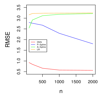
Figure 1: RMSE of first-stage estimator for DGP 1

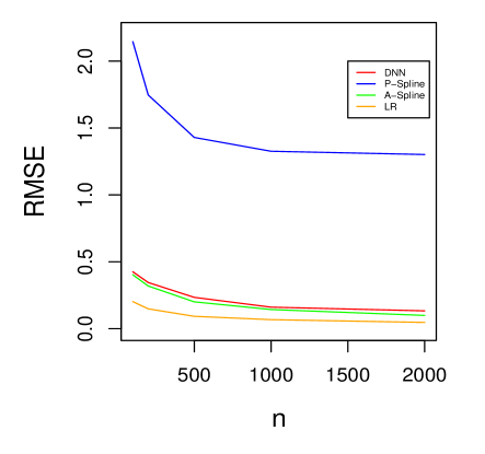
Figure 2: RMSE of first-stage estimator for DGP 2

We next evaluate the performance of the DNN estimators with different neural network structures by investigating the RMSE of $\widehat{f}$ in (3.2) with all the combinations of $W=5,10,20$ and $L=3,5,10$. It can be observed from Figures 3 and 4 that, the errors decrease when the sample size increases regardless of the choices of $W$ and $L$. Moreover, in terms of RMSE, the performance of $\widehat{f}$ is quite similar, especially when the sample size is large ($n\geq 1000$).

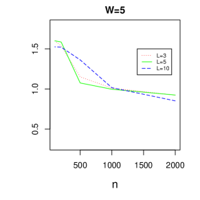
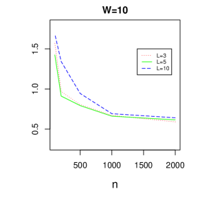
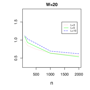
Figure 3: RMSE of the DNN estimator $\widehat{f}$ with different $(W,L)$ under DGP 1

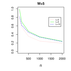
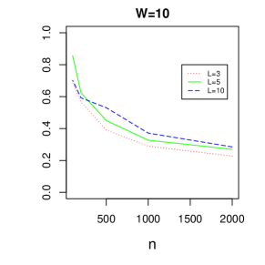
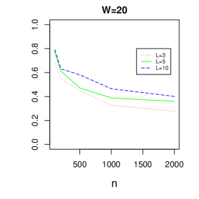
Figure 4: RMSE of the DNN estimator $\widehat{f}$ with different $(W,L)$ under DGP 2

6.2 Second-Stage Estimator

In addition to the second-stage estimator $\widehat{\beta}$ obtained through (4.2), we consider two other estimators of $\beta_{0}$ for comparison purpose. The first one is the ORACLE estimator that was obtained using $Y$ as the response and $f_{0}(\mathbf{Z})$ as the explanatory variable, and the second one is the naive OLS estimator that regressed $Y$ with respect to $X$. The former is unrealistic but used as a benchmark, while the second is known to be inconsistent due to endogeneity.

We use RMSE of $\widehat{\beta}$ as a criterion to evaluate the finite sample performance. Figure 5 suggests that in DGP 1, the LR, A-Spline, and OLS estimators have large RMSEs, which are not decreasing even when the sample size is relatively large ($n=2000$). This coincides with the theoretical analysis of the weak IV case in Example 4. In contrast, the P-Spline, DNN, and ORACLE estimators have relatively smaller error. Besides, the DNN estimator has a similar performance as the ORACLE estimator with a large sample size ($n\geq 1000$). However, when compared with the P-Spline estimator, the DNN estimator is uniformly better regardless of the sample size. In DGP 2, Figure 6 shows that the errors of all the estimators, except for the OLS, are significantly reduced when increasing the sample size. Moreover, the ORACLE, LR, A-Spline and DNN estimators have comparable performance when the sample size is great than $500$. However, when compared with the P-Spline estimator, the DNN estimator stands out under different sample sizes.

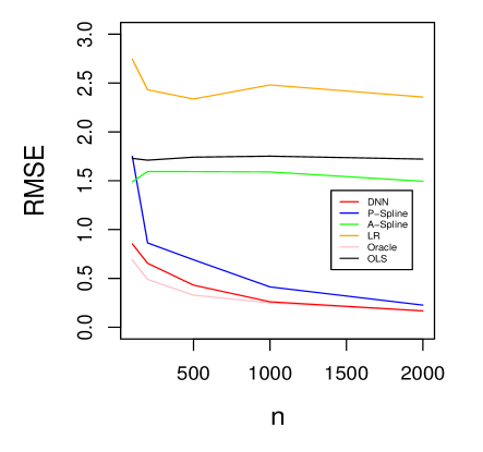
Figure 5: RMSE of second-stage estimator for DGP 1

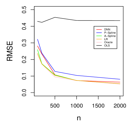
Figure 6: RMSE of second-stage estimator for DGP 2

We further conduct additional studies to evaluate the performance of $\widehat{\beta}$ using deep neural network with different $W$ and $L$. Figures 7 and 8 reveal that the DNN estimator is fairly stable to the choices of network structure. When sample size is great than $1000$, the RMSEs are very close for different $W$ and $L$.

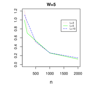
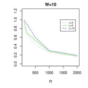
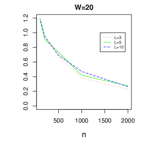
Figure 7: RMSE of the DNN estimator $\widehat{\beta}$ with different $(W,L)$ for DGP 1

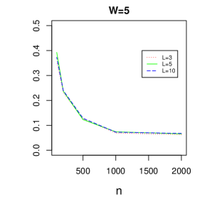
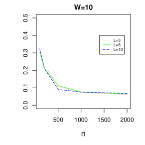
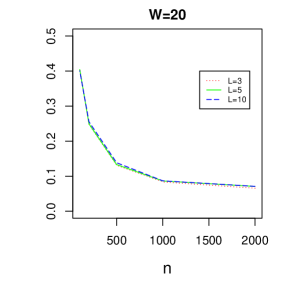
Figure 8: RMSE of the DNN estimator $\widehat{\beta}$ with different $(W,L)$ for DGP 2

6.3 Coverage Probability

We calculated the coverage probabilities of the proposed confidence interval in (4.1) to examine its empirical performance. The benchmark for comparison is based on the ORACLE estimator. Figures 9 and 10 report the coverage probabilities of the 95% confidence intervals based on DNN estimator and the ORACLE estimator under different sample sizes. In DGP 1, Figure 9 shows that when sample size is relatively large ($n\geq 1000$), the coverage probability of the DNN estimator is around $95\%$, while it is about $93\%$ for small sample. Figure 10 reveals that, in DGP 2, the performance of the DNN estimator and the ORACLE estimator are comparable, even when the sample size is around $500$. When the sample size is large ($n=2000$), the coverage probability stays around the 95% nominal level. The above findings confirm the validity of our theoretical results.

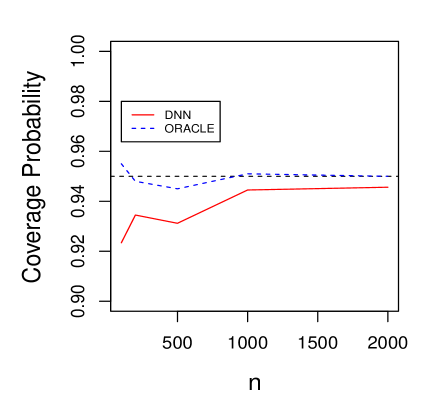
Figure 9: Coverage Probability for DGP 1

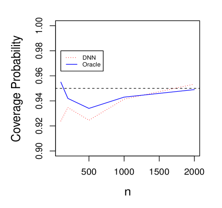
Figure 10: Coverage Probability for DGP 2

Additional simulation studies were conducted to evaluate the stability of the DNN estimator with different structures in terms of coverage probability. It can be seen from Figures 11 and 12 that, for various choices of $W$ and $L$, the difference of coverage probabilities is quite small (less than $2\%$).

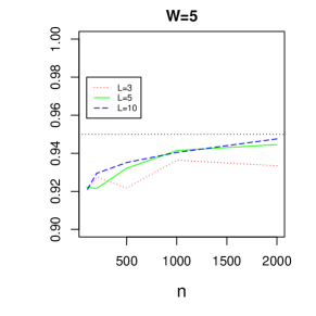
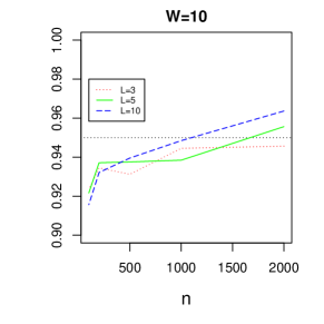
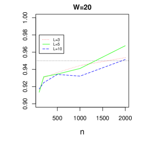
Figure 11: Coverage probability with different $(W,L)$ for DGP 1

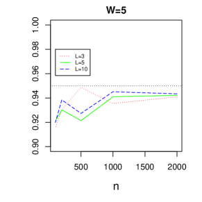
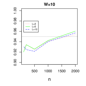
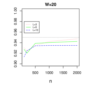
Figure 12: Coverage probability with different $(W,L)$ for DGP 2

7 Empirical Application

In this section, we apply the proposed estimation procedure to study automobile sales and price. Specifically, we consider the following model:

$$\textrm{sales}_{i}=\beta\times\textrm{price}_{i}+\epsilon,$$

where sales_i and price_i indicate the market sales and price of vehicle of type $i$. The instrumental variables we adopt are (a) a 0-1 valued variable indicating the air conditioning; (b) horsepower divided by weight; (c) miles per dollar measuring the routine costs; (d) size of the vehicle. Similar settings were also considered in Berry et al., (1995). After eliminating missing values, we keep 2217 types of automobiles in the dataset. We fit simple OLS, LR, A-Spline, P-Spline, and DNN based on the 2217 observations and summarize the results in Table 1. Several interesting findings can be observed. First, all the estimators are highly significant at 1% significance level. Second, without using instrumental variables, OLS gives an estimator of the coefficient $-0.0840$. Among the rest four instrumental variables estimators, the P-Spline estimator is more elastic than the OLS estimator, while LR, A-Spline, and DNN estimators are less elastic. Finally, we observe that LR and DNN estimators are almost equal, but the standard deviation of the DNN estimator is slightly smaller.

Table 1: Estimators of automobile price

	OLS	LR	A-Spline	P-Spline	DNN
$price$	-0.0840∗∗∗ (0.0029)	-0.0804∗∗∗ (0.0038)	-0.0814∗∗∗ (0.0037)	-0.0909∗∗∗ (0.0055)	-0.0805∗∗∗ (0.0036)

Note: *, **, and *** refer to significance at 10%, 5% and 1% level, respectively.

Appendix

For any $k$-dimensional vector $\mathbf{v}=(v_{1},\ldots,v_{k})^{\top}$ and real number $a$, we denote $\mathbf{v}+a=(v_{1}+a,\ldots,v_{k}+a)^{\top}$. Let $\mathbf{W}=(\mathbf{X},\mathbf{Z})$ be an independent copy of $\mathbf{W}_{i}=(\mathbf{X}_{i},\mathbf{Z}_{i})$ and for any function $f\mathrel{\mathop{\mathchar 58\relax}}\mathbb{R}^{d}\to\mathbb{R}$, we define norms $\|f\|_{\infty}=\sup_{\mathbf{z}}|f(\mathbf{z})|$ and $\|f\|_{n,\infty}=\sup_{1\leq i\leq n}|f(\mathbf{Z}_{i})|$. For matrix $A$, we define its Frobenius norm $\|A\|_{F}=\sqrt{\textrm{Tr}(A^{\top}A)}$. We recall the Rademacher Complexity (see Wainwright,, 2019) of function class $\mathcal{F}$ is defined as

$$\mathcal{R}_{n}\mathcal{F}=\mathbb{E}\bigg{(}\sup_{f\in\mathcal{F}}\frac{1}{n}\sum_{i=1}^{n}\eta_{i}f(\mathbf{Z}_{i})\bigg{|}\mathbf{Z}_{1},\ldots,\mathbf{Z}_{n}\bigg{)},$$

where $\eta_{i}$’s are i.i.d. Rademacher random variables which are independent of $\mathbf{Z}_{i}$’s. Moreover, we denote $\textrm{Pdim}(\mathcal{F})$ as the pseudo-dimension of $\mathcal{F}$ (see, Anthony and Bartlett,, 2009). For functions $f,g\mathrel{\mathop{\mathchar 58\relax}}\mathbb{R}^{d}\to\mathbb{R}$ and random variables $\zeta$ and $\xi$, we denote $\langle f,g\rangle_{n}=n^{-1}\sum_{i=1}^{n}f(\mathbf{Z}_{i})g(\mathbf{Z}_{i})$, $\langle\zeta,\xi\rangle_{n}=n^{-1}\sum_{i=1}^{n}\zeta_{i}\xi_{i}$ and $\langle\zeta,f\rangle_{n}=n^{-1}\sum_{i=1}^{n}\zeta_{i}f(\mathbf{Z}_{i})$, where $\zeta_{i},\xi_{i}$ are the observations of $\zeta,\xi$.

A.1 Some Preliminary Lemmas

Lemma A.1.

Suppose $(\zeta_{i},\mathbf{Z}_{i}),i=1,\ldots,n$ are i.i.d. observations and $\mathbb{E}(|\zeta_{i}|)<\infty$, then $\mathbb{E}(\zeta_{i}|\mathbf{Z}_{1},\ldots,\mathbf{Z}_{n})=\mathbb{E}(\zeta_{i}|\mathbf{Z}_{i})$ for all $i=1,\ldots,n$.

Proof.

We prove the case when $n=2$, and the extension to the case of general $n$ can be made analogically. We define $h_{1}=\mathbb{E}(\zeta_{1}|\mathbf{Z}_{1})$, $\mathcal{D}=\{A\in\mathcal{S}(\mathbf{Z}_{1},\mathbf{Z}_{2})\mathrel{\mathop{\mathchar 58\relax}}\mathbb{E}(\zeta_{1}I_{A})=\mathbb{E}(h_{1}I_{A})\}$, and $\mathcal{P}=\{A\times B\mathrel{\mathop{\mathchar 58\relax}}A\in\mathcal{S}(\mathbf{Z}_{1}),B\in\mathcal{S}(\mathbf{Z}_{2})\}$. Clearly, $\mathcal{P}$ is a $\pi$-system. Since $\mathbb{E}(|\zeta_{1}|)<\infty$, by Lebesgue’s dominated convergence theorem, it is not difficult to see $\mathcal{D}$ is a $\lambda$-system. Moreover, for $A\times B\in\mathcal{P}$, we can see

$$\mathbb{E}(\zeta_{1}I_{A\times B})=\mathbb{E}(\zeta_{1}I_{A}I_{B})=\mathbb{E}(\zeta_{1}I_{A})\mathbb{E}(I_{B})=\mathbb{E}(h_{1}I_{A})\mathbb{E}(I_{B})=\mathbb{E}(h_{1}I_{A}I_{B})=\mathbb{E}(h_{1}I_{A\times B}),$$

where we use the facts that $A\in\mathcal{S}(\mathbf{Z}_{1})$, $B\in\mathcal{S}(\mathbf{Z}_{2})$ and their independence. As a consequence of $\pi-\lambda$ monotone class theorem, we have $\mathcal{P}\subset\mathcal{D}$ and $\mathcal{S}(\mathbf{Z}_{1},\mathbf{Z}_{2})=\mathcal{S}(\mathcal{P})\subset\mathcal{D}\subset\mathcal{S}(\mathbf{Z}_{1},\mathbf{Z}_{2})$. By the definition of $\mathcal{D}$, we see that $\mathbb{E}(\zeta_{1}|\mathbf{Z}_{1},\mathbf{Z}_{2})=h_{1}$. ∎

Lemma A.2.

Suppose $(\zeta_{i},\mathbf{Z}_{i}),i=1,\ldots,n$ are i.i.d. observations and $\mathbb{E}(|\zeta_{i}|)<\infty$, then the random variables $\zeta_{1},\ldots,\zeta_{n}$ are conditionally mutually independent and identically distributed given $\mathbf{Z}_{1},\ldots,\mathbf{Z}_{n}$

Proof.

We prove the case when $n=2$, and the extension to the case of general $n$ can be made analogically. For any $a_{1},a_{2}\in\mathbb{R}$, we define $\delta_{i}=I(\zeta_{i}\leq a_{i})$ for $i=1,2$. Also we denote $h_{i}=\mathbb{E}(\delta_{i}|\mathbf{Z}_{1},\mathbf{Z}_{2})$, $\mathcal{D}=\{A\in\mathcal{S}(\mathbf{Z}_{1},\mathbf{Z}_{2})\mathrel{\mathop{\mathchar 58\relax}}\mathbb{E}(\delta_{1}\delta_{2}I_{A})=\mathbb{E}(h_{1}h_{2}I_{A})\}$, and $\mathcal{P}=\{A\times B\mathrel{\mathop{\mathchar 58\relax}}A\in\mathcal{S}(\mathbf{Z}_{1}),B\in\mathcal{S}(\mathbf{Z}_{2})\}$. It is not difficult to verify that $\mathcal{P}$ is a $\pi$-system and $\mathcal{D}$ is a $\lambda$-system. Moreover, due to Lemma A.1, we have $h_{i}\in\mathcal{S}(Z_{i})$. Therefore, for $A\times B\in\mathcal{P}$, we can verify

$$\mathbb{E}(\delta_{1}\delta_{2}I_{A\times B})=\mathbb{E}(\delta_{1}\delta_{2}I_{A}I_{B})=\mathbb{E}(\delta_{1}I_{A})\mathbb{E}(\delta_{2}I_{B}) =\mathbb{E}(h_{1}I_{A})\mathbb{E}(h_{2}I_{B})$$

$$=\mathbb{E}(h_{1}h_{2}I_{A}I_{B})$$

$$=\mathbb{E}(h_{1}h_{2}I_{A\times B}),$$

where we use the facts that $A\in\mathcal{S}(\mathbf{Z}_{1})$, $B\in\mathcal{S}(\mathbf{Z}_{2})$ and their independence. As a consequence of $\pi-\lambda$ monotone class theorem, we have $\mathcal{P}\subset\mathcal{D}$ and $\mathcal{S}(\mathbf{Z}_{1},\mathbf{Z}_{2})=\mathcal{S}(\mathcal{P})\subset\mathcal{D}\subset\mathcal{S}(\mathbf{Z}_{1},\mathbf{Z}_{2})$. By the definition of $\mathcal{D}$ and $h_{i}$, we see that $\mathbb{P}(\zeta_{1}\leq a_{1},\zeta_{2}\leq a_{2}|\mathbf{Z}_{1},\mathbf{Z}_{2})=h_{1}h_{2}=\mathbb{P}(\zeta_{1}\leq a_{1}|\mathbf{Z}_{1},\mathbf{Z}_{2})\mathbb{P}(\zeta_{2}\leq a_{2}|\mathbf{Z}_{1},\mathbf{Z}_{2})$. ∎

Lemma A.3.

Let $\mathcal{F}$ be a class of functions and $\phi\mathrel{\mathop{\mathchar 58\relax}}\mathbb{R}\to\mathbb{R}$ be a Lipschitz function with Lipschitz constant $K$, then

$$\mathbb{E}(\mathcal{R}_{n}\phi\circ\mathcal{F})\leq K\mathbb{E}(\mathcal{R}_{n}\mathcal{F}),$$

where $\phi\circ\mathcal{F}=\{\phi\circ f\mathrel{\mathop{\mathchar 58\relax}}f\in\mathcal{F}\}$.

Proof.

This is Proposition 5.28 in Wainwright, (2019). ∎

Lemma A.4.

Let $\mathcal{F}$ be a class of functions such that $|f|\leq B$ and $\textrm{Var}(f)\leq V$ for all $f\in\mathcal{F}$ and some $B,V\in\mathbb{R}$. Then for any $\eta>0$, with probability at least $1-2e^{-\eta}$,

$$\sup_{f\in\mathcal{F}}\bigg{|}(\mathbb{P}-\mathbb{P}_{n})[f]\bigg{|}\leq 3\mathbb{E}(\mathcal{R}_{n}\mathcal{F})+\sqrt{\frac{2V\eta}{n}}+\frac{4B\eta}{3n}.$$

Proof.

This is Theorem 2.1 in Bartlett et al., (2005). ∎

Lemma A.5.

Suppose $(\zeta_{i},\mathbf{Z}_{i}),i=1,\ldots,n$ are i.i.d. observations with $\mathbb{E}(\zeta_{i}|\mathbf{Z}_{i})=0$. Let $\mathcal{F}$ be a class of function with finite elements, and conditioning on $\mathbb{Z}$, $\|f\|_{n}\leq r$ for all $f\in\mathcal{F}$ and some $r>0$. Furthermore, if $\zeta_{1},\zeta_{2},\ldots,\zeta_{n}$ are conditionally independent given $\mathbb{Z}$ and $|\zeta_{i}|\leq B$ for some $B>0$, then

$$\mathbb{E}_{\mathbb{Z}}(\sup_{f\in\mathcal{F}}\langle f,\zeta\rangle_{n})\leq Br\sqrt{\frac{2\log(|\mathcal{F}|)}{n}}$$

Proof.

Conditioning on $\mathbb{Z}$, $\langle f,\zeta\rangle_{n}$ is $n^{-1/2}B\|f\|_{n}$-subgaussian due to the conditional independence of $\zeta_{1},\ldots,\zeta_{n}$. Furthermore, for any $\lambda>0$, it follows from Jensen’s inequality that

$$\exp\bigg{(}\lambda\mathbb{E}_{\mathbb{Z}}(\sup_{f\in\mathcal{F}}\langle f,\zeta\rangle_{n})\bigg{)} \leq \mathbb{E}_{\mathbb{Z}}\bigg{(}\exp(\lambda\sup_{f\in\mathcal{F}}\langle f,\zeta\rangle_{n})\bigg{)}$$

$$= \mathbb{E}_{\mathbb{Z}}\bigg{(}\sup_{f\in\mathcal{F}}\exp(\lambda\langle f,\zeta\rangle_{n})\bigg{)}$$

$$\leq \mathbb{E}_{\mathbb{Z}}\bigg{(}\sum_{f\in\mathcal{F}}\exp(\lambda\langle f,\zeta\rangle_{n})\bigg{)}$$

$$= \sum_{f\in\mathcal{F}}\mathbb{E}_{\mathbb{Z}}\bigg{(}\exp(\lambda\langle f,\zeta\rangle_{n})\bigg{)}$$

$$\leq \sum_{f\in\mathcal{F}}\exp\bigg{(}\frac{\lambda^{2}B^{2}\|f\|_{n}^{2}}{2n}\bigg{)}\leq|\mathcal{F}|\exp\bigg{(}\frac{\lambda^{2}B^{2}r^{2}}{2n}\bigg{)}.$$

As a consequence, it follows that

$$\mathbb{E}_{\mathbb{Z}}(\sup_{f\in\mathcal{F}}\langle f,\zeta\rangle_{n})\leq\frac{\lambda B^{2}r^{2}}{2n}+\frac{\log(|\mathcal{F}|)}{\lambda},\textrm{ for all }\lambda>0.$$

We complete the proof by setting $\lambda=\frac{\sqrt{2n\log(|\mathcal{F}|)}}{Br}$. ∎

Lemma A.6.

Suppose $(\zeta_{i},\mathbf{Z}_{i}),i=1,\ldots,n$ are i.i.d. observations with $\mathbb{E}(\zeta_{i}|\mathbf{Z}_{i})=0$. Let $\mathcal{F}$ be a class of functions such that conditioning on $\mathbb{Z}$, $\|f\|_{n}\leq r$ for all $f\in\mathcal{F}$ and some $r>0$. Furthermore, if $\zeta_{1},\zeta_{2},\ldots,\zeta_{n}$ are conditionally independent given $\mathbb{Z}$ and $|\zeta_{i}|\leq B$ for some $B>0$, then it follows that

$$\mathbb{E}_{\mathbb{Z}}(\sup_{f\in\mathcal{F}_{r}}\langle f,\zeta\rangle_{n})\leq\inf_{0<x<r}\bigg{\{}4x\sqrt{\frac{1}{n}\sum_{i=1}^{n}\mathbb{E}(\zeta_{i}^{2}|\mathbf{Z}_{i})}+12B\int_{x}^{r}\sqrt{\frac{\log\mathcal{N}(u,\mathcal{F}_{r},\|\cdot\|_{n})}{n}}du\bigg{\}}.$$

As a consequence, we have

$$\mathcal{R}_{n}\mathcal{F}_{r}\leq\inf_{0<x<r}\bigg{\{}4x+12\int_{x}^{r}\sqrt{\frac{\log\mathcal{N}(u,\mathcal{F}_{r},\|\cdot\|_{n})}{n}}du\bigg{\}}.$$

Proof.

Let $\alpha_{j}=2^{-j}r$ and $T_{j}$ be the a proper $alpha_{j}$-covering of $\mathcal{F}_{r}$ with respect to $\|\cdot\|_{n}$. For $f\in\mathcal{F}_{r}$, denote $\tau_{j}(f)\in T_{j}$ as the function such that $\|\tau_{j}(f)-f\|_{n}\leq\alpha_{j}$. For integer $N>0$, we have

$$f=f-\tau_{N}(f)+\sum_{j=1}^{N}(\tau_{j}(f)-\tau_{j-1}(f)),$$

here we denote $g_{0}=0$ for simplicity. Therefore, it follows that

$$\langle f,\zeta\rangle_{n} \leq \langle f-\tau_{N}(f),\zeta\rangle_{n}+\sum_{j=1}^{N}\langle\tau_{j}(f)-\tau_{j-1}(f),\zeta\rangle_{n}$$ (A.1)

$$\leq \|\zeta\|_{n}\|f-\tau_{N}(f)\|_{n}+\sum_{j=1}^{N}\langle\tau_{j}(f)-\tau_{j-1}(f),\zeta\rangle_{n}$$

$$\leq \alpha_{N}\|\zeta\|_{n}+\sum_{j=1}^{N}\langle\tau_{j}(f)-\tau_{j-1}(f),\zeta\rangle_{n}.$$

Now notice that

$$\|\tau_{j}(f)-\tau_{j-1}(f)\|_{n}\leq\|\tau_{j}(f)-f\|_{n}+\|\tau_{j-1}(f)-f\|_{n}\leq\alpha_{j}+\alpha_{j-1}=3\alpha_{j}.$$

Therefore, apply Lemma A.5 to the class $\{f_{j}-f_{j-1}\mathrel{\mathop{\mathchar 58\relax}}\|f_{j}-f_{j-1}\|_{n}\leq 3\alpha_{j},f_{j}\in T_{j},f_{j-1}\in T_{j-1}\}$, it follows that

$$\mathbb{E}_{\mathbb{Z}}\bigg{(}\sup_{f\in\mathcal{F}_{r}}\langle\tau_{j}(f)-\tau_{j-1}(f),\zeta\rangle_{n}\bigg{)} \leq 3\alpha_{j}B\sqrt{\frac{2\log(|T_{j}||T_{j-1}|)}{n}}$$

$$\leq 6\alpha_{j}B\sqrt{\frac{\log(|T_{j}|)}{n}}$$

$$\leq 12B(\alpha_{j}-\alpha_{j+1})\sqrt{\frac{\log(|T_{j}|)}{n}}$$

$$\leq 12B(\alpha_{j}-\alpha_{j+1})\sqrt{\frac{\log\mathcal{N}(\alpha_{j},\mathcal{F}_{r},\|\cdot\|_{n})}{n}}$$

$$\leq 12B\int_{\alpha_{j+1}}^{\alpha_{j}}\sqrt{\frac{\log\mathcal{N}(u,\mathcal{F}_{r},\|\cdot\|_{n})}{n}}du.$$

Above inequality and (A.1) together imply that

$$\mathbb{E}_{\mathbb{Z}}(\sup_{f\in\mathcal{F}_{r}}\langle f,\zeta\rangle_{n})\leq\alpha_{N}\mathbb{E}_{\mathbf{Z}}(\|\zeta\|_{n})+12B\int_{\alpha_{N+1}}^{\alpha_{0}}\sqrt{\frac{\log\mathcal{N}(u,\mathcal{F}_{r},\|\cdot\|_{n})}{n}}du.$$

Now pick $N$ such that, $\alpha_{N}>2\epsilon$ and $\alpha_{N+1}\leq 2\epsilon$. Therefore, $\alpha_{N}=2\alpha_{N+1}\leq 4\epsilon$ and $\alpha_{N+1}=\alpha_{N}/2>\epsilon$. Hence, we conclude that

$$\mathbb{E}_{\mathbb{Z}}(\sup_{f\in\mathcal{F}_{r}}\langle f,\zeta\rangle_{n})\leq 4\epsilon\sqrt{\frac{1}{n}\sum_{i=1}^{n}\mathbb{E}(\zeta_{i}^{2}|\mathbf{Z}_{i})}+12B\int_{\epsilon}^{r}\sqrt{\frac{\log\mathcal{N}(u,\mathcal{F}_{r},\|\cdot\|_{n})}{n}}du,$$

where we use the inequality $\mathbb{E}_{\mathbb{Z}}(\|\zeta\|_{n})\leq\sqrt{\mathbb{E}_{\mathbb{Z}}(\|\zeta\|_{n}^{2})}$ and Lemma A.1. Since $\epsilon>0$ is arbitrary, we finish the proof. ∎

Lemma A.7.

For a class of function $\mathcal{F}$, if $n\geq\textrm{Pdim}(\mathcal{F})$ and $\max_{1\leq i\leq n}\|f(\mathbf{Z}_{i})\|\leq C$ for all $f\in\mathcal{F}$ and some constant $C>0$, then it follows that

$$\log N(x,\mathcal{F},\|\cdot\|_{n,\infty})\leq\textrm{Pdim}(\mathcal{F})\log\bigg{(}\frac{2enC}{x\textrm{Pdim}(\mathcal{F})}\bigg{)}\leq\textrm{Pdim}(\mathcal{F})\log\bigg{(}\frac{2enC}{x}\bigg{)}.$$

Moreover for deep neural network class, it holds that

$$\textrm{Pdim}(\mathcal{F}_{d,1}(L,W))\leq\textrm{VC}(\mathcal{F}_{d+1,1}(L+1,W+1))\leq cL(LW^{2}+Wd)\log(LW^{2}+Wd),$$

for some universal constant .

Proof.

The first result is Theorem 12.2 in Anthony and Bartlett, (2009). The second one follows from Theorem 14.1 in Anthony and Bartlett, (2009) and Theorem 6 in Bartlett et al., (2019). ∎

Lemma A.8.

Let $\mathbf{a}_{1},\mathbf{b}_{2},\ldots,\mathbf{a}_{n},\mathbf{b}_{n}$ be real vectors of the same dimension. Then it follows that

$$\bigg{\|}\frac{1}{n}\sum_{i=1}^{n}\mathbf{a}_{i}\mathbf{b}_{i}^{\top}\bigg{\|}_{F}^{2}\leq\frac{1}{n}\sum_{i=1}^{n}\|\mathbf{a}_{i}\|_{2}^{2}\times\frac{1}{n}\sum_{i=1}^{n}\|\mathbf{b}_{i}\|_{2}^{2}.$$

Proof.

Denote $\mathbf{a}_{i}=(a_{i1},\ldots,a_{ik})^{\top}$ and $\mathbf{b}_{i}=(b_{i1},\ldots,b_{ik})^{\top}$ for $i=1,\ldots,n$. By definition of Frobenius norm and Cauchy–Schwarz inequality, we have

$$\bigg{\|}\sum_{i=1}^{n}\mathbf{a}_{i}\mathbf{b}_{i}^{\top}\bigg{\|}_{F}^{2}=\sum_{j=1}^{k}\sum_{s=1}^{k}\bigg{(}\sum_{i=1}^{n}a_{ij}b_{is}\bigg{)}^{2}\leq\sum_{j=1}^{k}\sum_{s=1}^{k}\sum_{i=1}^{n}a_{ij}^{2}\sum_{i=1}^{n}b_{is}^{2}=\sum_{i=1}^{n}\|\mathbf{a}_{i}\|_{2}^{2}\times\sum_{i=1}^{n}\|\mathbf{b}_{i}\|_{2}^{2}.$$

∎

A.2 DNN Approximation

The proof of approximation results of DNN, we mainly rely on the result in Lu et al., (2020). We borrow the following notation from their paper. For given $K\in\mathbb{Z}_{+}$ and $\delta>0$ with $\delta<\frac{1}{K}$, define the trifling region of $[0,1]^{d}$ as follows:

$$\Omega(K,\delta,d)\mathrel{\mathop{\mathchar 58\relax}}=\bigcup_{i=1}^{d}\bigg{\{}\mathbf{z}=(z_{1},\ldots,z_{d})^{\top}\mathrel{\mathop{\mathchar 58\relax}}x_{i}\in\bigcup_{k=1}^{K-1}\bigg{(}\frac{k}{K}-\delta,\frac{k}{K}\bigg{)}\bigg{\}}.$$ (A.2)

Lemma A.9.

For any $N,L\in\mathbb{Z}_{+}$, there exists a network $\phi_{\times}\in\mathcal{F}_{2,1}(L+1,9N)$ such that

1. $|\phi_{\times}(x,y)-xy|\leq 12N^{-L}$ for all $x,y\in[0,1]$;

2. $|\phi_{\times}(x,y)|\leq 1$ for all $x,y\in[0,1]$.

Proof.

By Lemma 5.2 in Lu et al., (2020), there exists a $\widetilde{\phi}_{\times}\in\mathcal{F}_{2,1}(L,9N)$ such that

$$|\widetilde{\phi}_{\times}(x,y)-xy|\leq 6N^{-L},\;\;\textrm{ for all }x,y\in[0,1].$$ (A.3)

Let $\delta\mathrel{\mathop{\mathchar 58\relax}}=6N^{-L}$, and we further define

$$\phi_{\times}(x,y)=\frac{\sigma(\widetilde{\phi}_{\times}(x,y))}{1+\delta}.$$

Direct examination implies

$$|\phi_{\times}(x,y)-xy|=\bigg{|}\frac{\sigma(\widetilde{\phi}_{\times}(x,y))}{1+\delta}-xy\bigg{|}=\begin{cases}|xy|&\textrm{ if }\widetilde{\phi}_{\times}(x,y)<0\\ \bigg{|}\frac{\widetilde{\phi}_{\times}(x,y)}{1+\delta}-xy\bigg{|}&\textrm{ if }\widetilde{\phi}_{\times}(x,y)\geq 0\end{cases}.$$

Notice by (A.3), if $\widetilde{\phi}_{\times}(x,y)<0$ implies $|xy|\leq 6N^{-L}=\delta$, and

$$\bigg{|}\frac{\widetilde{\phi}_{\times}(x,y)}{1+\delta}-xy\bigg{|}=\bigg{|}\frac{\widetilde{\phi}_{\times}(x,y)-xy-\delta xy}{1+\delta}\bigg{|}\leq\frac{2\delta}{1+\delta}\leq 2\delta.$$

Therefore, we show that $|\widetilde{\phi}_{\times}(x,y)-xy|\leq 2\delta=12N^{-L}$ for all $x,y\in[0,1]$. Moreover, since $\widetilde{\phi}_{\times}(x,y)\leq 1+6N^{-L}\leq 1+\delta$, it holds that $\phi_{\times}(x,y)\leq 1$. Finally, it is trivial to see that $\phi_{\times}(x,y)\in\mathcal{F}_{2,1}(L+1,9N)$. ∎

Lemma A.10.

For any $N,L,d\in\mathbb{Z}_{+}$, there exists a network $\phi_{\times}^{d}\in\mathcal{F}_{d,1}((L+1)(d-1)+d-2,9N+d-2)$ such that

1. $|\phi_{\times}^{d}(\mathbf{z})-\prod_{i=1}^{d}z_{i}|\leq 12(d-1)N^{-L}$ for all $\mathbf{z}=(z_{1},\ldots,z_{d})^{\top}\in[0,1]^{d}$;

2. $|\phi_{\times}^{d}(\mathbf{z})|\leq 1$ for all $\mathbf{z}=(z_{1},\ldots,z_{d})^{\top}\in[0,1]^{d}$.

Proof.

For simplicity, we prove the case when $d=3$. By Lemma A.9, there exist a network $\phi_{\times}\in\mathcal{F}_{2,1}(L+1,9N)$ such that $|\phi_{\times}(z_{1},z_{2})-z_{1}z_{2}|\leq 12N^{-L}$. To pass the value of $z_{3}$ to next layer, we can add one more channel to store the $z_{3}$. Therefore, we use $\phi_{\times}(\phi_{\times}(z_{1},z_{2}),z_{3})$ to approximate the products, and the error can be calculated as follows:

$$|\phi_{\times}(\phi_{\times}(z_{1},z_{2}),z_{3})-z_{1}z_{2}z_{3}| \leq |\phi_{\times}(\phi_{\times}(z_{1},z_{2}),z_{3})-\phi_{\times}(z_{1},z_{2})z_{3}|+|\phi_{\times}(z_{1},z_{2})z_{3}-z_{1}z_{2}z_{3}|$$

$$\leq 12N^{-L}+12N^{-L}\leq 24N^{-L}.$$

Finally, it is not difficult to verify that this neural network has $2(L+1)+1$ hidden layers and width $9N+1$. ∎

Lemma A.11.

For any $N,L\in\mathbb{Z}_{+}$ and $\bm{\gamma}=(\gamma_{1},\ldots,\gamma_{d})\in\mathbb{Z}^{d}$, there exists a network $P_{\bm{\gamma}}\in\mathcal{F}_{d,1}$ with $(L+2)(|\bm{\gamma}|-1)$ hidden layers and width $9N+|\bm{\gamma}|-2$ such that

1. $|P_{\bm{\gamma}}(\mathbf{z})-\mathbf{z}^{\bm{\gamma}}|\leq 12(|\bm{\gamma}|-1)N^{-L}$ for all $\mathbf{z}=(z_{1},\ldots,z_{d})^{\top}\in[0,1]^{d}$;

2. $|P_{\bm{\gamma}}(\mathbf{z})|\leq 1$ for all $\mathbf{z}=(z_{1},\ldots,z_{d})^{\top}\in[0,1]^{d}$.

Proof.

First step we pass the input value $\mathbf{z}$ to next layer as follows:

$$\mathbf{z}\to(\underbrace{z_{1},\ldots,z_{1}}_{\gamma_{1}\textrm{ times }},\underbrace{z_{2},\ldots,z_{2}}_{\gamma_{2}\textrm{ times }},\ldots,\underbrace{z_{d-1},\ldots,z_{d-1}}_{\gamma_{d-1}\textrm{ times }},\underbrace{z_{d},\ldots,z_{d}}_{\gamma_{d}\textrm{ times }}).$$

Next we apply the neural network defined in Lemma A.10 to obtain the desired result. Clearly, this neural network consistent of $(L+1)(|\bm{\gamma}|-1)+|\bm{\gamma}|-1$ hidden layers and width $9N+|\bm{\gamma}|-2$. ∎

Lemma A.12.

For any $N,L,d\in\mathbb{Z}_{+}$ and $\delta>0$ with $K=\left\lfloor N^{1/d}\right\rfloor^{2}\left\lfloor L^{2/d}\right\rfloor$ and $\delta\leq\frac{1}{3K}$, there exits a neural network $\psi_{\textrm{map}}\in\mathcal{F}_{1,1}(4L+4,4N+5)$ such that

$$\psi_{\textrm{map}}(x)=\frac{k}{K},\textrm{ if }x\in\bigg{[}\frac{k}{K},\frac{k+1}{K}-\delta I(x<K-1)\bigg{]}\textrm{ for }k=0,1,\ldots,K-1.$$

Proof.

This is Proposition 4.3 in Lu et al., (2020). ∎

Lemma A.13.

Given any $N,L,m\in\mathbb{Z}_{+}$ and $\xi_{i}\in[0,1]$ for $i=0,1,\ldots,N^{2}L^{2}-1$, there exists a neural network $\phi_{\textrm{fit}}$ with depth $(5L+8){\lceil\log_{2}(2L)\rceil}$ and width $8m(2N+3){\lceil\log_{2}(4N)\rceil}$ such that

1. $|\phi_{\textrm{fit}}(i)-\xi_{i}|\leq N^{-2m}L^{-2m}$, for $i=0,1,\ldots,N^{2}L^{2}-1$;

2. $0\leq\phi_{\textrm{fit}}(x)\leq 1$ for all $x\in\mathbb{R}$.

Proof.

This is Proposition 4.4 in Lu et al., (2020). ∎

Lemma A.14.

Suppose $f\mathrel{\mathop{\mathchar 58\relax}}[0,1]^{d}\to\mathbb{R}$ be $(p,1)$-Hölder smooth for some $p>0$, then for all positive integers $M,N$, there exists a neural network $g\in\mathcal{F}_{d,1}(L,W)$ with

$$L=18{\lceil p\rceil}^{2}(M+3){\lceil\log_{2}(2M)\rceil}$$

and

$$W=40({\lceil p\rceil}+d+2)^{d+1}(N+2){\lceil\log_{2}(4N)\rceil}$$

such that

$$|f(\mathbf{z})-g(\mathbf{z})|\leq(86+d8^{p})(p+1)^{d+1}N^{-2p/d}M^{-2p/d}\quad\textrm{ for all }\;\mathbf{z}\in[0,1]^{d}\backslash\Omega(K,\delta,d),$$

where $K=\left\lfloor N^{1/d}\right\rfloor^{2}\left\lfloor M^{2/d}\right\rfloor$ and $0<\delta<\frac{1}{3K}$ can be chosen arbitrary.

Proof.

Step 1: For notational simplicity, we denote $m=\left\lfloor p\right\rfloor$, the largest integer strictly smaller than $p$. For each $\bm{\theta}=(\theta_{1},\ldots,\theta_{d})^{\top}\in\{0,1,\ldots,K-1\}^{d}$, we define

$$Q_{\bm{\theta}}\mathrel{\mathop{\mathchar 58\relax}}=\bigg{\{}\mathbf{z}=(z_{1},\ldots,z_{d})^{\top}\mathrel{\mathop{\mathchar 58\relax}}z_{i}\in\bigg{[}\frac{\theta_{i}}{K},\frac{\theta_{i}+1}{K}-\delta I(\theta_{i}<K-1)\bigg{]},i=1,\ldots,d\bigg{\}}.$$

Clearly, $[0,1]^{d}\backslash\Omega(K,\delta,d)=\cup_{\bm{\theta}}Q_{\bm{\theta}}$. By Lemma A.12, there exists a neural network $\psi_{\textrm{map}}\in\mathcal{F}_{1,1}(4M+4,4N+5)$ such that

$$\psi_{\textrm{map}}(z)=\frac{k}{K},\textrm{ if }z\in\bigg{[}\frac{k}{K},\frac{k+1}{K}-\delta I(x<K-1)\bigg{]}\textrm{ for }k=0,1,\ldots,K-1.$$

Therefore, by parallelizing $d$ above networks, we can obtain a neural network

$$\bm{\psi}_{\textrm{map}}(\mathbf{z})\mathrel{\mathop{\mathchar 58\relax}}=(\psi_{\textrm{map}}(z_{1}),\ldots,\psi_{\textrm{map}}(z_{d}))^{\top}\in\mathcal{F}_{d,d}(4M+4,d(4N+5))$$

such that

$$\bm{\psi}_{\textrm{map}}(\mathbf{z})=\frac{\bm{\theta}}{K},\textrm{ if }\mathbf{z}\in Q_{\bm{\theta}}\textrm{ for all }\bm{\theta}\in\{0,1,\ldots,K-1\}^{d}.$$ (A.4)

Step 2: For all $\bm{\gamma}=(\gamma_{1},\ldots,\gamma_{d})^{\top}\in\mathbb{Z}^{d}$ with $|\bm{\gamma}|\leq m$, by Lemma A.11, there exists a neural network $P_{\bm{\gamma}}\in\mathcal{F}_{d,1}$ with depth $(2(m+1)(M+1)+2)(m-1)$ and width $9N+m-2$ such that

$$|P_{\bm{\gamma}}(\mathbf{z})-\mathbf{z}^{\bm{\gamma}}|\leq 12(m-1)N^{-2(m+1)(M+1)}\;\textrm{ for all }\mathbf{z}=(z_{1},\ldots,z_{d})^{d}\in[0,1]^{d}.$$ (A.5)

Moreover, for each $i=0,1,\ldots,K^{d}-1$, we define mapping

$$\bm{\vartheta}(i)\mathrel{\mathop{\mathchar 58\relax}}=(\vartheta_{1},\ldots,\vartheta_{d})^{\top}\in\{0,1,\ldots,K-1\}^{d}$$ (A.6)

such that $\sum_{j=1}^{d}\vartheta_{j}K^{j-1}=i$. This can be done, since this is a bijection. For each $\bm{\gamma}=(\gamma_{1},\ldots,\gamma_{d})^{\top}\in\mathbb{Z}^{d}$ with $|\bm{\gamma}|\leq m$, define

$$\xi_{\bm{\gamma},i}=\bigg{[}\partial^{\bm{\gamma}}f\bigg{(}\frac{\bm{\vartheta(i)}}{K}\bigg{)}+1\bigg{]}/2\;\textrm{ for }i=0,1,\ldots,K^{d}-1.$$ (A.7)

We can see that $\xi_{\bm{\gamma},i}\in[0,1]$, as $f$ is $(p,1)$-Hölder smooth. By Lemma A.13 and the fact that $K^{d}\leq N^{2}M^{2}$, there exist a neural network $\phi_{\bm{\gamma}}$ with depth $(5M+8){\lceil\log_{2}(2M)\rceil}$ and width $8(m+1)(2N+3){\lceil\log_{2}(4N)\rceil}$ that

$$|\phi_{\bm{\gamma}}(i)-\xi_{\bm{\gamma},i}|\leq N^{-2(m+1)}M^{-2(m+1)}\;\textrm{ for all }i=0,1,\ldots,K^{d}-1\textrm{ and }|\bm{\gamma}|\leq m.$$ (A.8)

Step 3: Using above networks, we further define

$$\Phi_{\bm{\gamma}}(\mathbf{z})=\phi_{\bm{\gamma}}(\sum_{j=1}^{d}z_{j}K^{j})\;\textrm{ for all }\mathbf{z}=(z_{1},\ldots,z_{d})^{\top}\in[0,1]^{d}.$$ (A.9)

Clearly, $\Phi_{\bm{\gamma}}\in\mathcal{F}_{d,1}$ has depth at most $(5M+8){\lceil\log_{2}(2M)\rceil}+2$ and width at most $8(m+1)(2N+3){\lceil\log_{2}(4N)\rceil}+d$.

Notice if $\mathbf{z}\in Q_{\bm{\theta}}$ for some $\bm{\theta}=(\theta_{1},\ldots,\theta_{d})^{\top}\in\{0,1,\ldots,K-1\}^{d}$, then by (A.4) and (A.6), we have following mapping:

$$\mathbf{z}\xrightarrow{\bm{\psi}_{\textrm{map}}}\frac{\bm{\theta}}{K}\xrightarrow{\Phi_{\bm{\gamma}}}\phi_{\bm{\gamma}}(i),$$

where the integer $i=\sum_{j=1}^{d}\theta_{j}K^{j-1}$ by (A.6). As a consequence of (A.7) and (A.8), it follows that

$$\bigg{|}\Phi_{\bm{\gamma}}\circ\bm{\psi}_{\textrm{map}}(\mathbf{z})-\bigg{[}\partial^{\bm{\gamma}}f\bigg{(}\frac{\bm{\theta}}{K}\bigg{)}+1\bigg{]}/2\bigg{|}\leq N^{-2(m+1)}M^{-2(m+1)}\;\;\textrm{ if }\mathbf{z}\in Q_{\bm{\theta}}.$$ (A.10)

Finally, we define our network to be

$$g(\mathbf{z})=2\sum_{|\bm{\gamma}|\leq m}\phi_{\times}\bigg{(}\frac{\Phi_{\bm{\gamma}}\circ\bm{\psi}_{\textrm{map}}(\mathbf{z})}{\bm{\gamma}!},P_{\bm{\gamma}}(\mathbf{z}-\bm{\psi}_{\textrm{map}}(\mathbf{z}))\bigg{)}-\sum_{|\bm{\gamma}|\leq m}\frac{P_{\bm{\gamma}}(\mathbf{z}-\bm{\psi}_{\textrm{map}}(\mathbf{z}))}{\bm{\gamma}!},$$

where $\phi_{\times}\in\mathcal{F}_{2,1}(2(m+1)(M+1)+1,9N)$ is the product neural network in Lemma A.9 such that

$$|\phi_{\times}(x,y)-xy|\leq 12N^{-2(m+1)(M+1)}.$$ (A.11)

Step 4: For any $\mathbf{z}\in Q_{\bm{\theta}}$, let $\mathbf{h}\mathrel{\mathop{\mathchar 58\relax}}=\mathbf{z}-\frac{\bm{\theta}}{K}=\mathbf{z}-\frac{\bm{\psi}_{\textrm{map}}(\mathbf{z})}{K}$. By Taylor’s Theorem, we can quantify the bound of $|f(\mathbf{z})-g(\mathbf{z})|$ by

$$\bigg{|}\sum_{|\bm{\gamma}|\leq m}\frac{\partial^{\bm{\gamma}}f(\bm{\psi}_{\textrm{map}}(\mathbf{z}))}{\bm{\gamma}!}\mathbf{h}^{\bm{\gamma}}+\sum_{|\bm{\gamma}|=m}\frac{\partial^{\bm{\gamma}}f(\bm{\psi}_{\textrm{map}}(\mathbf{z})+\xi_{\mathbf{z}}\mathbf{h})}{\bm{\gamma}!}\mathbf{h}^{\bm{\gamma}}-\sum_{|\bm{\gamma}|=m}\frac{\partial^{\bm{\gamma}}f(\bm{\psi}_{\textrm{map}}(\mathbf{z}))}{\bm{\gamma}!}\mathbf{h}^{\bm{\gamma}}-g(\mathbf{z})\bigg{|}$$

$$\leq S_{1}+S_{2},$$

where $\xi_{\mathbf{z}}\in[0,1]$ and

$$S_{1}=\bigg{|}\sum_{|\bm{\gamma}|=m}\frac{\partial^{\bm{\gamma}}f(\bm{\psi}_{\textrm{map}}(\mathbf{z})+\xi_{\mathbf{z}}\mathbf{h})}{\bm{\gamma}!}\mathbf{h}^{\bm{\gamma}}-\sum_{|\bm{\gamma}|=m}\frac{\partial^{\bm{\gamma}}f(\bm{\psi}_{\textrm{map}}(\mathbf{z}))}{\bm{\gamma}!}\mathbf{h}^{\bm{\gamma}}\bigg{|},\;S_{2}=\bigg{|}\sum_{|\bm{\gamma}|\leq m}\frac{\partial^{\bm{\gamma}}f(\bm{\psi}_{\textrm{map}}(\mathbf{z}))}{\bm{\gamma}!}\mathbf{h}^{\bm{\gamma}}-g(\mathbf{z})\bigg{|}.$$

By the definition of $(p,1)$-Hölder smooth, it follows that

$$S_{1}\leq\sum_{|\bm{\gamma}|=m}\frac{\|\xi_{\mathbf{z}}\mathbf{h}\|_{2}^{p-m}}{\bm{\gamma}!}\mathbf{h}^{\bm{\gamma}}\leq\frac{d(m+1)^{d}}{\bm{\gamma}!}K^{-p}\leq d(m+1)^{d}K^{-p}.$$

For the term $S_{2}$, we have $S_{2}=S_{21}+S_{22}$ with

$$S_{21} = 2\sum_{|\bm{\gamma}|\leq m}\frac{\partial^{\bm{\gamma}}f(\bm{\psi}_{\textrm{map}}(\mathbf{z}))+1}{2\bm{\gamma}!}\mathbf{h}^{\bm{\gamma}}-\sum_{|\bm{\gamma}|\leq m}2\phi_{\times}\bigg{(}\frac{\Phi_{\bm{\gamma}}\circ\bm{\psi}_{\textrm{map}}(\mathbf{z})}{\bm{\gamma}!},P_{\bm{\gamma}}(\mathbf{z}-\bm{\psi}_{\textrm{map}}(\mathbf{z}))\bigg{)},$$

$$S_{22} = \sum_{|\bm{\gamma}|\leq m}\frac{1}{\bm{\gamma}!}\mathbf{h}^{\bm{\gamma}}-\sum_{|\bm{\gamma}|\leq m}\frac{P_{\bm{\gamma}}(\mathbf{z}-\bm{\psi}_{\textrm{map}}(\mathbf{z}))}{\bm{\gamma}!}.$$

Direct examination leads to the following bound:

$$S_{21} \leq 2\bigg{|}\sum_{|\bm{\gamma}|\leq m}\frac{\partial^{\bm{\gamma}}f(\bm{\psi}_{\textrm{map}}(\mathbf{z}))+1}{2\bm{\gamma}!}\mathbf{h}^{\bm{\gamma}}-\sum_{|\bm{\gamma}|\leq m}\frac{\Phi_{\bm{\gamma}}\circ\bm{\psi}_{\textrm{map}}(\mathbf{z})}{\bm{\gamma}!}P_{\bm{\gamma}}(\mathbf{z}-\bm{\psi}_{\textrm{map}}(\mathbf{z}))\bigg{|}$$

$$+2\bigg{|}\sum_{|\bm{\gamma}|\leq m}\frac{\Phi_{\bm{\gamma}}\circ\bm{\psi}_{\textrm{map}}(\mathbf{z})}{\bm{\gamma}!}P_{\bm{\gamma}}(\mathbf{z}-\bm{\psi}_{\textrm{map}}(\mathbf{z}))-\sum_{|\bm{\gamma}|\leq m}2\phi_{\times}\bigg{(}\frac{\Phi_{\bm{\gamma}}\circ\bm{\psi}_{\textrm{map}}(\mathbf{z})}{\bm{\gamma}!},P_{\bm{\gamma}}(\mathbf{z}-\bm{\psi}_{\textrm{map}}(\mathbf{z}))\bigg{)}\bigg{|}$$

$$\leq 2\sum_{|\bm{\gamma}|\leq m}\bigg{|}\frac{\partial^{\bm{\gamma}}f(\bm{\psi}_{\textrm{map}}(\mathbf{z}))+1}{2\bm{\gamma}!}\mathbf{h}^{\bm{\gamma}}-\frac{\Phi_{\bm{\gamma}}\circ\bm{\psi}_{\textrm{map}}(\mathbf{z})}{\bm{\gamma}!}\mathbf{h}^{\bm{\gamma}}\bigg{|}$$

$$+2\sum_{|\bm{\gamma}|\leq m}\bigg{|}\frac{\Phi_{\bm{\gamma}}\circ\bm{\psi}_{\textrm{map}}(\mathbf{z})}{\bm{\gamma}!}\mathbf{h}^{\bm{\gamma}}-\frac{\Phi_{\bm{\gamma}}\circ\bm{\psi}_{\textrm{map}}(\mathbf{z})}{\bm{\gamma}!}P_{\bm{\gamma}}(\mathbf{z}-\bm{\psi}_{\textrm{map}}(\mathbf{z}))\bigg{|}$$

$$+2\sum_{|\bm{\gamma}|\leq m}\sup_{x,y\in[0,1]}|xy-\phi_{\times}(x,y)|$$

$$\leq 2(m+1)^{d}N^{-2(m+1)}M^{-2(m+1)}+24(m+1)^{d}(1+N^{-2(m+1)}M^{-2(m+1)})(m-1)N^{-2(m+1)(M+1)}$$

$$+24(m+1)^{d}N^{-2(m+1)(M+1)}$$

$$\leq 2(m+1)^{d}N^{-2(m+1)}M^{-2(m+1)}+72(m+1)^{d+1}N^{-2(m+1)(M+1)},$$

where we use (A.5), (A.10) and (A.11). Similarly, using (A.5), we have

$$S_{22} \leq \sum_{|\bm{\gamma}|\leq m}\bigg{|}\mathbf{h}^{\bm{\gamma}}-P_{\bm{\gamma}}(\mathbf{z}-\bm{\psi}_{\textrm{map}}(\mathbf{z}))\bigg{|}\leq 12(m+1)^{d+1}N^{-2(m+1)(M+1)}.$$

As a consequence of the bounds of $S_{1},S_{21}$ and $S_{22}$, we conclude that for $\mathbf{z}\in Q_{\bm{\theta}}$, it holds that

$$|f(\mathbf{z})-g(\mathbf{z})| \leq d(m+1)^{d}K^{-p}+2(m+1)^{d}N^{-2(m+1)}M^{-2(m+1)}+84(m+1)^{d+1}N^{-2(m+1)(M+1)}$$

$$\leq d8^{p}(m+1)^{d}N^{-2p/d}M^{-2p/d}+2(m+1)^{d}N^{-2(m+1)}M^{-2(m+1)}+$$

$$+84(m+1)^{d+1}N^{-2(m+1)}N^{-2(m+1)M}$$

$$\leq d8^{p}(m+1)^{d}N^{-2p/d}M^{-2p/d}+2(m+1)^{d}N^{-2(m+1)}M^{-2(m+1)}+$$

$$+84(m+1)^{d+1}N^{-2(m+1)}M^{-2(m+1)}$$

$$\leq (86+d8^{p})(m+1)^{d+1}N^{-2p/d}M^{-2p/d},$$

where we use the fact that $K=\left\lfloor N^{1/d}\right\rfloor^{2}\left\lfloor M^{2/d}\right\rfloor\geq N^{2/d}M^{2/d}/8$.

Step 5: We will demonstrate how to implement $g$ using neural network. We denote the set $\Gamma=\{\bm{\gamma}\in\mathbb{N}^{d}\mathrel{\mathop{\mathchar 58\relax}}|\bm{\gamma}|\leq m\}$. By basic Combinatorics, we now $|\Gamma|={m+d-1\choose m-1}$. For simplicity, we set $|\Gamma|=J$ and index the element in $\Gamma$ as $\bm{\gamma}_{1},\ldots,\bm{\gamma}_{J}$. For each $\bm{\gamma}in\Gamma$, we define

$$h_{\bm{\gamma}}(\mathbf{z})=\frac{\Phi_{\bm{\gamma}}\circ\bm{\psi}_{\textrm{map}}(\mathbf{z})}{\bm{\gamma}!}\quad\quad\textrm{ and }\quad\quad f_{\bm{\gamma}}(\mathbf{z})=P_{\bm{\gamma}}(\mathbf{z}-\bm{\psi}_{\textrm{map}}(\mathbf{z})).$$

By (A.4), (A.5) and (A.9), it is not difficult to see $h_{\bm{\gamma}}$ has at most depth

$$4M+4+(5L+8){\lceil\log_{2}(2M)\rceil}+2+2\leq 10(M+2){\lceil\log_{2}(2M)\rceil}$$

and width

$$d(4N+5)+8(m+1)(2N+3){\lceil\log_{2}(4N)\rceil}+d\leq 16(m+d+1)(N+2){\lceil\log_{2}(4N)\rceil}.$$

Similarly, we can show $f_{\bm{\gamma}}$ has at most depth

$$4M+4+1+[2(m+1)(M+2)+2](m-1)+1\leq 6(m+1)^{2}(M+3)$$

and width

$$d(4N+5)+d+9N+m-2\leq(4d+9)(N+2)+m.$$

Now, we parallelize all the $h_{\bm{\gamma}}$’s and $f_{\bm{\gamma}}$’s together, we can obtain a neural network

$$g_{1}\mathrel{\mathop{\mathchar 58\relax}}=(h_{\bm{\gamma}_{1}},\ldots,h_{\bm{\gamma}_{J}},f_{\bm{\gamma}_{1}},\ldots,f_{\bm{\gamma}_{J}})^{\top}\in\mathcal{F}_{d,2J}$$

with at most $16(m+1)^{2}(M+3){\lceil\log_{2}(2M)\rceil}$ hidden layers and at most width $40J(m+d+3)(N+2){\lceil\log_{2}(4N)\rceil}$.

Next for each $\bm{\gamma}\in\Gamma$, using the product neural network in (A.11), we define

$$s_{\bm{\gamma}}=2\phi_{\times}(h_{\bm{\gamma}},f_{\bm{\gamma}}),$$

and use the outputs of $g_{1}$ to construct a neural network $g_{2}\circ g_{1}$ such that

$$g_{2}\circ g_{1}\mathrel{\mathop{\mathchar 58\relax}}=(s_{\bm{\gamma}_{1}},\ldots,s_{\bm{\gamma}_{J}},f_{\bm{\gamma}_{1}},\ldots,f_{\bm{\gamma}_{J}})^{\top}\in\mathcal{F}_{d,2J},$$

which will have at most depth

$$16(m+1)^{2}(M+3){\lceil\log_{2}(2M)\rceil}+2(m+1)(M+1)+1+1\leq 18(m+1)^{2}(M+3){\lceil\log_{2}(2M)\rceil}$$

and at most width $40J(m+d+3)(N+2){\lceil\log_{2}(4N)\rceil}$.

Finally, we make a linear combination using the outputs of $g_{2}\circ g_{1}$ to obtain the final neural network, which will require one more hidden layer. We will finish the proof if we notice $J\leq(m+1)^{d}$. ∎

Lemma A.15.

Given $\varepsilon>0$, $L,W,K\in\mathbb{Z}_{+}$, and $\delta>0$ with $\delta<\frac{1}{3K}$, assume $f$ is continuous on $[0,1]^{d}$. Suppose there is a neural network $\widetilde{g}\in\mathcal{F}_{d,1}(L,W)$ such that

$$|f(\mathbf{z})-\widetilde{g}(\mathbf{z})|\leq\varepsilon\quad\textrm{ for all }\mathbf{z}\in[0,1]^{d}\backslash\Omega(K,\delta,d),$$

then there exists a neural network $g\in\mathcal{F}_{d,1}(L+2d,3^{d}(N+3))$ such that

$$|f(\mathbf{z})-g(\mathbf{z})|\leq\varepsilon+d\omega_{f}(\delta)\quad\textrm{ for all }\mathbf{z}\in[0,1]^{d},$$

where $\omega_{f}(\delta)=\sup\{|f(\mathbf{x})-f(\mathbf{y})|\mathrel{\mathop{\mathchar 58\relax}}\|\mathbf{x}-\mathbf{y}\|_{2}\leq\delta,\mathbf{x},\mathbf{y}\in[0,1]^{d}\}$.

Lemma A.16.

Suppose $f\mathrel{\mathop{\mathchar 58\relax}}[0,1]^{d}\to\mathbb{R}$ be $(p,C)$-Hölder smooth for some $p,C>0$, then for all positive intergers $M,N$, there exists a neural network $g\in\mathcal{F}_{d,1}(L,W)$ with

$$L=54{\lceil p\rceil}^{2}(M+3){\lceil\log_{2}(2M)\rceil}\;\;\textrm{ and }\;\;W=40({\lceil p\rceil}+d+2)^{d+1}3^{d}(N+2){\lceil\log_{2}(4N)\rceil}+3^{d+1}$$

such that

$$\sup_{\mathbf{z}\in[0,1]^{d}}|f(\mathbf{z})-g(\mathbf{z})|\leq C(86+d8^{p}+d)(p+1)^{d+1}N^{-2p/d}M^{-2p/d}.$$

Proof.

Define $\widetilde{f}=C^{-1}f$, so $\widetilde{f}$ is $(p,1)$-Hölder smooth. Set $K=\left\lfloor N^{1/d}\right\rfloor^{2}\left\lfloor M^{2/d}\right\rfloor$ and choose $\delta\in(0,\frac{1}{3K})$ such that $\omega_{\widetilde{f}}(\delta)\leq N^{-2p/d}L^{-2p/d}$. This can be done, as

$$\omega_{f}(\delta)\leq\begin{cases}\delta&\textrm{ if }p\geq 1\\ \delta^{p}&\textrm{ if }p<1\\ \end{cases}.$$

By Lemma A.14, there exists a neural network $\widetilde{g}_{1}$ with $18{\lceil p\rceil}^{2}(M+3){\lceil\log_{2}(2M)\rceil}$ hidden layers and width $40({\lceil p\rceil}+d+2)^{d+1}(N+2){\lceil\log_{2}(4N)\rceil}$ such that $|\widetilde{f}(\mathbf{z})-\widetilde{g}_{1}(\mathbf{z})|\leq(86+d8^{p})(m+1)^{d+1}N^{-2p/d}M^{-2p/d}$ for all $\mathbf{z}\in[0,1]^{d}\backslash\Omega(K,\delta,d)$. By Lemma A.15, there exists a neural network $\widetilde{g}_{2}$ with $54{\lceil p\rceil}^{2}(M+3){\lceil\log_{2}(2M)\rceil}$ hidden layers and width $40({\lceil p\rceil}+d+2)^{d+1}3^{d}(N+2){\lceil\log_{2}(4N)\rceil}+3^{d+1}$ such that

$$|\widetilde{f}(\mathbf{z})-\widetilde{g}_{2}(\mathbf{z})| \leq (86+d8^{p})(p+1)^{d+1}N^{-2p/d}M^{-2p/d}+dN^{-2p/d}L^{-2p/d}$$

$$\leq (86+d8^{p}+d)(p+1)^{d+1}N^{-2p/d}M^{-2p/d}\;\;\textrm{ for all }\mathbf{z}\in[0,1]^{d}.$$

As a consequence, the neural network $g\mathrel{\mathop{\mathchar 58\relax}}=Cg_{2}$, which has the same architecture as $g_{2}$, is the desired neural network. ∎

Lemma A.17.

Suppose $h\mathrel{\mathop{\mathchar 58\relax}}[0,1]^{d}\to[0,1]$ be $(p,C)$-Hölder smooth for some $p,C>0$, then for all positive integers $M,N$, there exists a neural network $h_{\textrm{net}}\in\mathcal{F}_{d,1}(L,W)$ with

$$L=54{\lceil p\rceil}^{2}(M+3){\lceil\log_{2}(2M)\rceil}+1\quad\textrm{ and }\quad W=40({\lceil p\rceil}+d+2)^{d+1}3^{d}(N+2){\lceil\log_{2}(4N)\rceil}+3^{d+1}$$

such that $0\leq h_{\textrm{net}}(\mathbf{z})\leq 1$ and

$$\sup_{\mathbf{z}\in[0,1]^{d}}|h(\mathbf{z})-h_{\textrm{net}}(\mathbf{z})|\leq 2(86+d8^{p}+d)(p+1)^{d+1}N^{-2p/d}M^{-2p/d}.$$

Proof.

By Lemma A.16, there exists $\widetilde{h}_{\textrm{net}}\in\mathcal{F}_{d,1}(\widetilde{L},\widetilde{W})$ with

$$\widetilde{L}=54{\lceil p\rceil}^{2}(M+3){\lceil\log_{2}(2M)\rceil}\;\;\textrm{ and }\;\;\widetilde{W}=40({\lceil p\rceil}+d+2)^{d+1}3^{d}(N+2){\lceil\log_{2}(4N)\rceil}+3^{d+1}$$

such that

$$\sup_{\mathbf{z}\in[0,1]^{d}}|\widetilde{h}_{\textrm{net}}(\mathbf{z})-h(\mathbf{z})|\leq(86+d8^{p}+d)(p+1)^{d+1}N^{-2p/d}M^{-2p/d}\;\;\textrm{ for all }N,M\in\mathbb{Z}_{+}.$$ (A.12)

Let $\delta=(86+d8^{p}+d)(p+1)^{d+1}N^{-2p/d}M^{-2p/d}$ and define $h_{\textrm{net}}(\mathbf{z})=\sigma(\widetilde{h}(\mathbf{z}))/(1+2\delta)$, which is always non-negative. If $\widetilde{h}(\mathbf{z})\leq 0$, then by (A.12), we have $h(\mathbf{z})-\delta\leq\widetilde{h}(\mathbf{z})\leq 0$, which further leads to $0\leq h(\mathbf{z})\leq\delta$. Therefore, it follows that

$$|h_{\textrm{net}}(\mathbf{z})-h(\mathbf{z})|= \begin{cases}\bigg{|}\frac{\widetilde{h}(\mathbf{z})}{1+\delta}-h(\mathbf{z})\bigg{|}&\textrm{ if }\widetilde{h}(\mathbf{z})>0\\ h(\mathbf{z})&\textrm{ if }\widetilde{h}(\mathbf{z})\leq 0\\ \end{cases}.$$

Combining above, we conclude that $\sup_{\mathbf{z}\in[0,1]^{d}}|h_{\textrm{net}}(\mathbf{z})-h(\mathbf{z})|\leq 2\delta$. Also by (A.12), it yields that $h_{\textrm{net}}(\mathbf{z})\leq|\widetilde{h}(\mathbf{z})|/(1+2\delta)\leq 1$. Clearly, $h_{\textrm{net}}$ can be implemented by adding one more layer to $\widetilde{h}(\mathbf{z})$. ∎

Lemma A.18.

Suppose $f\in\mathcal{C}\mathcal{S}(L_{*},\mathbf{d},\mathbf{t},\mathbf{p},\mathbf{a},\mathbf{b},C)$, for all positive integers $M_{0},N_{0},\ldots,M_{L_{*}},N_{L_{*}}$, there exists $\widetilde{f}\in\mathcal{F}_{d,1}(L_{*}+\sum_{i=0}^{L_{*}}L_{i},\max_{0\leq i\leq L_{*}}W_{i}d_{i+1})$ with

$$L_{i}=54{\lceil p_{i}\rceil}^{2}(M_{i}+3){\lceil\log_{2}(2M_{i})\rceil}+1\;\;\textrm{ and }\;W_{i}=40({\lceil p_{i}\rceil}+t_{i}+2)^{t_{i}+1}3^{t_{i}}(N_{i}+2){\lceil\log_{2}(4N_{i})\rceil}+3^{t_{i}+1}$$

such that

$$\|\widetilde{f}-{f}\|_{\infty}\leq c\sum_{i=0}^{L_{*}}(M_{i}N_{i})^{-2p_{i}\prod_{s=i+1}^{L_{*}}(p_{s}\wedge 1)/t_{i}},$$

where constant $c$ is free of $d,M$ and $N$. As a consequence, if $(L,W)\to\infty$, then there exists $\widetilde{f}\in\mathcal{F}_{d,1}(L,W)$ such that

$$\|\widetilde{f}-{f}\|_{\infty}\leq c\max_{1\leq i\leq L_{*}}\bigg{(}\frac{LW}{\log(L)\log(W)}\bigg{)}^{-\frac{2p_{i}\prod_{s=i+1}^{L_{*}}(p_{s}\wedge 1)}{t_{i}}}=c\bigg{(}\frac{LW}{\log(L)\log(W)}\bigg{)}^{-\frac{2p^{*}}{t^{*}}}.$$

where the constant $c$ is free of $d,L$ and $W$. Moreover, if $\mathbf{f}=(f_{1},f_{2},\ldots,f_{q})^{\top}$ with each $f_{i}\in\mathcal{C}\mathcal{S}(L_{*},\mathbf{d},\mathbf{t},\mathbf{p},\mathbf{a},\mathbf{b},C)$, then there exists $\mathbf{f}^{*}=(f_{1}^{*},f_{2}^{*},\ldots,f_{q}^{*})^{\top}\in\mathcal{F}_{d,q}(L,W)$ suhc that

$$\|{f}_{s}^{*}-{f}_{s}\|_{\infty}\leq c\bigg{(}\frac{LW}{\log(L)\log(W)}\bigg{)}^{-\frac{2p^{*}}{t^{*}}}\quad\textrm{ for all }s=1,\ldots,d,$$

where the constant $c$ is free of $d,L$ and $W$.

Proof.

Step 1: We will rewrite $f$ as composition of functions $\mathbf{h}_{i}$’s, which are defined as follows:

$$\mathbf{h}_{i}(\mathbf{z}) = \frac{\mathbf{g}_{i}((b_{i}-a_{i})\mathbf{z}+a_{i})-a_{i+1}}{b_{i+1}-a_{i+1}}\;\;\;\textrm{ for }\mathbf{z}\in[0,1]^{d_{i}}\textrm{ and }i=0,1,\ldots,L_{*}-1,$$

$$\mathbf{h}_{L_{*}}(\mathbf{z}) = \mathbf{g}_{L_{*}}((b_{L_{*}}-a_{L_{*}})\mathbf{z}+a_{L_{*}})\;\;\;\textrm{ for }\mathbf{z}\in[0,1]^{d_{L_{*}}}.$$

By above definition, we can see the range of $\mathbf{h}_{i}$ is $[0,1]^{d_{i+1}}$ for $i=0,\ldots,L_{*}-1$ and the domain of $\mathbf{h}_{i}$ is $[0,1]^{d_{i}}$ for $i=0,\ldots,L_{*}$. It is not difficult to verify following equality:

$$f(\mathbf{z})=\mathbf{h}_{L_{*}}\circ\ldots\circ\mathbf{h}_{0}\bigg{(}\frac{\mathbf{z}-a_{0}}{b_{0}-a_{0}}\bigg{)}\;\;\;\textrm{ for }\mathbf{z}\in[a_{0},b_{0}]^{d}.$$

Step 2: Let $h_{i,1},\ldots,h_{i,d_{i+1}}$ be the elements of $\mathbf{h}_{i}$. Since all $g_{i,j}$’s are $(p_{i},C)$-Hölder smooth and only relying on $t_{i}$ variables, we can see that $h_{i,j}$’s are $(p_{i},K)$-Hölder smooth with $K=C\sum_{i=0}^{L_{*}-1}(b_{i}-a_{i})/(b_{i+1}-a_{i+1})+b_{L_{*}}-a_{L_{*}}$. By Lemmas A.16 and A.17, there exists $\widetilde{h}_{i,j}\in\mathcal{F}_{t_{i},1}(L_{i},W_{i})$ with

$$L_{i}=54{\lceil p_{i}\rceil}^{2}(M_{i}+3){\lceil\log_{2}(2M_{i})\rceil}+1\;\;\textrm{ and }\;W_{i}=40({\lceil p_{i}\rceil}+t_{i}+2)^{t_{i}+1}3^{t_{i}}(N_{i}+2){\lceil\log_{2}(4N_{i})\rceil}+3^{t_{i}+1}$$

such that

$$\sup_{\mathbf{z}\in[0,1]^{t_{i}}}|\widetilde{h}_{i,j}(\mathbf{z})-h_{i,j}(\mathbf{z})|\leq c_{i}N^{-2p_{i}/t_{i}}M^{-2p_{i}/t_{i}},$$ (A.13)

where $c_{i}=K(86+t_{i}8^{p_{i}}+t_{i})(p_{i}+1)^{t_{i}+1}$.
Step 3: For each $i=0,\ldots,L_{*}$, we further define $\widetilde{\mathbf{h}}_{i}=(\widetilde{h}_{i,1},\ldots,\widetilde{h}_{i,d_{i+1}})^{\top}$. Moreover, let

$$\widetilde{f}(\mathbf{z})=\widetilde{\mathbf{h}}_{L_{*}}\circ\ldots\circ\widetilde{\mathbf{h}}_{0}\bigg{(}\frac{\mathbf{z}-a_{0}}{b_{0}-a_{0}}\bigg{)}\;\;\;\textrm{ for }\mathbf{z}\in[a_{0},b_{0}]^{d}.$$

Next we will quantify the difference between $\widetilde{f}(\mathbf{z})$ and $f(\mathbf{z})$.

$$|\widetilde{f}(\mathbf{z})-{f}(\mathbf{z})| = \bigg{|}\widetilde{\mathbf{h}}_{L_{*}}\circ\widetilde{\mathbf{h}}_{L_{*}-1}\circ\ldots\circ\widetilde{\mathbf{h}}_{0}\bigg{(}\frac{\mathbf{z}-a_{0}}{b_{0}-a_{0}}\bigg{)}-\mathbf{h}_{L_{*}}\circ\mathbf{h}_{L_{*}-1}\circ\ldots\circ\mathbf{h}_{0}\bigg{(}\frac{\mathbf{z}-a_{0}}{b_{0}-a_{0}}\bigg{)}\bigg{|}$$

$$\leq \bigg{|}\widetilde{\mathbf{h}}_{L_{*}}\circ\widetilde{\mathbf{h}}_{L_{*}-1}\circ\ldots\circ\widetilde{\mathbf{h}}_{0}\bigg{(}\frac{\mathbf{z}-a_{0}}{b_{0}-a_{0}}\bigg{)}-\mathbf{h}_{L_{*}}\circ\widetilde{\mathbf{h}}_{L_{*}-1}\circ\ldots\circ\widetilde{\mathbf{h}}_{0}\bigg{(}\frac{\mathbf{z}-a_{0}}{b_{0}-a_{0}}\bigg{)}\bigg{|}$$

$$+\bigg{|}{\mathbf{h}}_{L_{*}}\circ\widetilde{\mathbf{h}}_{L_{*}-1}\circ\ldots\circ\widetilde{\mathbf{h}}_{0}\bigg{(}\frac{\mathbf{z}-a_{0}}{b_{0}-a_{0}}\bigg{)}-\mathbf{h}_{L_{*}}\circ\mathbf{h}_{L_{*}-1}\circ\ldots\circ\mathbf{h}_{0}\bigg{(}\frac{\mathbf{z}-a_{0}}{b_{0}-a_{0}}\bigg{)}\bigg{|}$$

$$\leq \sup_{\mathbf{z}\in[0,1]^{d_{L_{*}}}}|\widetilde{\mathbf{h}}_{L_{*}}(\mathbf{z})-\mathbf{h}_{L_{*}}(\mathbf{z})|$$

$$+K\bigg{\|}\widetilde{\mathbf{h}}_{L_{*}-1}\circ\ldots\circ\widetilde{\mathbf{h}}_{0}\bigg{(}\frac{\mathbf{z}-a_{0}}{b_{0}-a_{0}}\bigg{)}-\mathbf{h}_{L_{*}-1}\circ\ldots\circ\mathbf{h}_{0}\bigg{(}\frac{\mathbf{z}-a_{0}}{b_{0}-a_{0}}\bigg{)}\bigg{\|}_{2}^{p_{L_{*}}\wedge 1},$$

where we use the fact that $\mathbf{h}_{L_{*}}$ is $(p_{L_{*}},K)$-Hölder smooth and $d_{L_{*}+1}=1$. Moreover, we can show the following holds for $i=1,\ldots,L_{*}-1$ and $r\in(0,1]$:

$$\bigg{\|}\widetilde{\mathbf{h}}_{i}\circ\widetilde{\mathbf{h}}_{i-1}\circ\ldots\circ\widetilde{\mathbf{h}}_{0}\bigg{(}\frac{\mathbf{z}-a_{0}}{b_{0}-a_{0}}\bigg{)}-\mathbf{h}_{i}\circ\mathbf{h}_{i-1}\circ\ldots\circ\mathbf{h}_{0}\bigg{(}\frac{\mathbf{z}-a_{0}}{b_{0}-a_{0}}\bigg{)}\bigg{\|}_{2}^{r}$$

$$\leq \bigg{\|}\widetilde{\mathbf{h}}_{i}\circ\widetilde{\mathbf{h}}_{i-1}\circ\ldots\circ\widetilde{\mathbf{h}}_{0}\bigg{(}\frac{\mathbf{z}-a_{0}}{b_{0}-a_{0}}\bigg{)}-\mathbf{h}_{i}\circ\widetilde{\mathbf{h}}_{i-1}\circ\ldots\circ\widetilde{\mathbf{h}}_{0}\bigg{(}\frac{\mathbf{z}-a_{0}}{b_{0}-a_{0}}\bigg{)}\bigg{\|}_{2}^{r}$$

$$+\bigg{\|}{\mathbf{h}}_{i}\circ\widetilde{\mathbf{h}}_{i-1}\circ\ldots\circ\widetilde{\mathbf{h}}_{0}\bigg{(}\frac{\mathbf{z}-a_{0}}{b_{0}-a_{0}}\bigg{)}-\mathbf{h}_{i}\circ\mathbf{h}_{i-1}\circ\ldots\circ\mathbf{h}_{0}\bigg{(}\frac{\mathbf{z}-a_{0}}{b_{0}-a_{0}}\bigg{)}\bigg{\|}_{2}^{r}$$

$$\leq \bigg{(}\sum_{j=1}^{d_{i+1}}\|\widetilde{h}_{i,j}-h_{i,j}\|^{2}_{\infty}\bigg{)}^{\frac{r}{2}}$$

$$+\bigg{(}\sum_{j=1}^{d_{i+1}}\bigg{|}h_{i,j}\circ\widetilde{\mathbf{h}}_{i-1}\circ\ldots\circ\widetilde{\mathbf{h}}_{0}\bigg{(}\frac{\mathbf{z}-a_{0}}{b_{0}-a_{0}}\bigg{)}-h_{i,j}\circ\mathbf{h}_{i-1}\circ\ldots\circ\mathbf{h}_{0}\bigg{(}\frac{\mathbf{z}-a_{0}}{b_{0}-a_{0}}\bigg{)}\bigg{|}^{2}\bigg{)}^{\frac{r}{2}}$$

$$\leq d_{i+1}\sup_{1\leq j\leq d_{i+1}}\|\widetilde{h}_{i,j}-h_{i,j}\|_{\infty}^{r}$$

$$+\sum_{j=1}^{d_{i+1}}\bigg{|}h_{i,j}\circ\widetilde{\mathbf{h}}_{i-1}\circ\ldots\circ\widetilde{\mathbf{h}}_{0}\bigg{(}\frac{\mathbf{z}-a_{0}}{b_{0}-a_{0}}\bigg{)}-h_{i,j}\circ\mathbf{h}_{i-1}\circ\ldots\circ\mathbf{h}_{0}\bigg{(}\frac{\mathbf{z}-a_{0}}{b_{0}-a_{0}}\bigg{)}\bigg{|}^{r}$$

$$\leq d_{i+1}\sup_{\mathbf{z}\in[0,1]^{d_{i}}}\|\widetilde{\mathbf{h}}_{i}(\mathbf{z})-\mathbf{h}_{i}(\mathbf{z})\|_{\infty}^{r}$$

$$+d_{i+1}K^{p_{i+1}\wedge 1}\bigg{\|}\widetilde{\mathbf{h}}_{i-1}\circ\ldots\circ\widetilde{\mathbf{h}}_{0}\bigg{(}\frac{\mathbf{z}-a_{0}}{b_{0}-a_{0}}\bigg{)}-\mathbf{h}_{i-1}\circ\ldots\circ\mathbf{h}_{0}\bigg{(}\frac{\mathbf{z}-a_{0}}{b_{0}-a_{0}}\bigg{)}\bigg{\|}_{2}^{r(p_{i}\wedge 1)}.$$

Finally, by induction, we conclude that

$$|\widetilde{f}(\mathbf{z})-{f}(\mathbf{z})| \leq K^{1+\sum_{i=1}^{L_{*}}p_{i}\wedge 1}\prod_{i=1}^{L_{*}}d_{i}\sum_{i=0}^{L_{*}}\sup_{1\leq j\leq d_{i+1}}\|\widetilde{h}_{i,j}-h_{i,j}\|_{\infty}^{\prod_{s=i+1}^{L_{*}}(p_{s}\wedge 1)},$$

where we use the convention $\prod_{s=L_{*}+1}^{L_{*}}(p_{i}\wedge 1)=1$. By (A.13), we show that

$$|\widetilde{f}(\mathbf{z})-{f}(\mathbf{z})| \leq K^{1+\sum_{i=1}^{L_{*}}p_{i}\wedge 1}\prod_{i=1}^{L_{*}}d_{i}\sum_{i=0}^{L_{*}}(c_{i}M_{i}^{-2p_{i}/t_{i}}N_{i}^{-2p_{i}/t_{i}})^{\prod_{s=i+1}^{L_{*}}(p_{s}\wedge 1)}$$

$$\leq K^{1+\sum_{i=1}^{L_{*}}p_{i}\wedge 1}\prod_{i=1}^{L_{*}}d_{i}\sum_{i=0}^{L_{*}}c_{i}^{\prod_{s=i+1}^{L_{*}}(p_{s}\wedge 1)}\sum_{i=0}^{L_{*}}(M_{i}N_{i})^{-2p_{i}\prod_{s=i+1}^{L_{*}}(p_{s}\wedge 1)/t_{i}}.$$

Therefore, we prove the bound with $c=K^{1+\sum_{i=1}^{L_{*}}p_{i}\wedge 1}\prod_{i=1}^{L_{*}}d_{i}\sum_{i=0}^{L_{*}}c_{i}^{\prod_{s=i+1}^{L_{*}}(p_{s}\wedge 1)}$, which is free of $d_{0},L,W$.
Step 4: We will show $\widetilde{f}$ indeed can be implemented by a deep neural network. We add the one more layer to transform the corresponding variables of $\widetilde{h}_{0,j}$ ($t_{i}$ variables) and parallelize all the $\widetilde{h}_{0,j}$’s (the total number is $d_{1}$) to implement $\widetilde{\mathbf{h}}_{0}((\mathbf{z}-a_{0})/(b_{0}-a_{0}))$, which can be verified that

$$\widetilde{\mathbf{h}}_{0}((\mathbf{z}-a_{0})/(b_{0}-a_{0}))\in\mathcal{F}_{d_{0},d_{1}}(L_{0}+1,d_{1}W_{0}),$$

where $L_{i},W_{i}$ are defined in Step 2. Now we use the outputs of $\widetilde{\mathbf{h}}_{0}((\mathbf{z}-a_{0})/(b_{0}-a_{0}))$ as inputs and parallelize all the $\widetilde{h}_{1,j}$’s (the total number is $d_{2}$) to implement $\widetilde{\mathbf{h}}_{1}\circ\widetilde{\mathbf{h}}_{0}((\mathbf{z}-a_{0})/(b_{0}-a_{0}))$. It can be verified that

$$\widetilde{\mathbf{h}}_{1}\circ\widetilde{\mathbf{h}}_{0}((\mathbf{z}-a_{0})/(b_{0}-a_{0}))\in\mathcal{F}_{d_{0},d_{2}}(L_{0}+L_{1}+2,\max\{d_{1}W_{0},d_{2}W_{1}\}).$$

By induction, we concluded that $\widetilde{f}\in\mathcal{F}_{d,1}(L_{*}+\sum_{i=0}^{L_{*}}L_{i},\max_{0\leq i\leq L_{*}}W_{i}d_{i+1})$, here we use the fact $d_{0}=d$ and $d_{L_{*}+1}=1$.
Step 5: Now we will prove the second result. It is not difficult to verify $M_{i}\asymp L_{i}\log^{-1}(L_{i})$ and $N_{i}\asymp W_{i}^{-1}\log(W_{i})$. Specifically, we choose $L_{0}=L_{1}=\cdots=L_{L_{*}}\asymp L$, $W_{0}=W_{1}=\cdots=W_{L_{*}}\asymp W$, then the desired result follows.
Step 6: The third result can be easily obtained by parallelizing $q$ deep neural networks in Step 5. ∎

A.3 Proof of Results in Section 4

Proof of Lemma 1.

Denote the degree of smoothness of $\mathbf{g}_{i}\circ\ldots\circ\mathbf{g}_{0}$ as $\widetilde{p}_{i}$. By Juditsky et al., (2009), the smoothness of $\mathbf{g}_{1}\circ\mathbf{g}_{0}$ is

$$\widetilde{p}_{1}\mathrel{\mathop{\mathchar 58\relax}}=p_{0}p_{1}\wedge p_{0}\wedge p_{1}=p_{0}(p_{1}\wedge 1)\wedge p_{1}\leq p_{0}(p_{1}\wedge 1).$$

Above equation and Juditsky et al., (2009) further imply

$$\widetilde{p}_{2}\mathrel{\mathop{\mathchar 58\relax}}=\widetilde{p}_{1}p_{2}\wedge\widetilde{p}_{1}\wedge p_{2}=\widetilde{p}_{1}(p_{2}\wedge 1)\wedge p_{2}\leq p_{0}(p_{1}\wedge 1)(p_{2}\wedge 1).$$

By induction, we conclude that

$$\widetilde{p}_{i}\leq p_{0}\prod_{k=1}^{i}(p_{k}\wedge 1),$$ (A.14)

here for convenience, we define $\widetilde{p}_{0}=p_{0}$. Similarly, if we define the smoothness of $\mathbf{g}_{L_{*}}\circ\ldots\circ\mathbf{g}_{i}$ as $\bar{p}_{i}$, we can show that

$$\bar{p}_{i}\leq p_{i}\prod_{k=i+1}^{L_{*}}(p_{k}\wedge 1)=p_{i}^{*},$$ (A.15)

here for convenience, we define $\bar{p}_{L_{*}}=p_{L_{*}}$. By Juditsky et al., (2009), (A.14) and (A.15), it follows that

$$p=\widetilde{p}_{i-1}\bar{p}_{i}\wedge\widetilde{p}_{i-1}\wedge\bar{p}_{i}\leq\bar{p}_{i}\leq p_{i}^{*},\quad\quad\textrm{ for all }i=1,\ldots,L_{*}.$$

Finally, notice $p=\widetilde{p}_{L_{*}}\leq p_{0}\prod_{k=1}^{L_{*}}(p_{k}\wedge 1)=p_{L_{*}}^{*}$, we conclude that

$$p\leq\min_{0\leq i\leq L_{*}}p_{i}^{*}.$$

∎

Lemma A.19.

Let $\zeta_{s}=X_{s}-f_{0,s}(\mathbf{Z})$ for $s=1,\ldots,q$. Under Assumption A1, the following holds for any positive integer $k$, real number $B>0$ and $s=1,\ldots,q$:

$$\mathbb{E}\bigg{(}|\zeta_{s}|^{k}I(|\zeta_{s}|>B)\bigg{)} \leq \kappa_{2}e^{\kappa_{1}C}\bigg{(}\frac{k+1}{\kappa_{1}}\bigg{)}^{k}e^{-\frac{\kappa_{1}B}{(k+1)}}.$$

Similarly, under Assumption A2, it holds that

$$\mathbb{E}\bigg{(}|\epsilon|^{k}I(|\epsilon|>B)\bigg{)}\leq\kappa_{4}\bigg{(}\frac{k+1}{\kappa_{3}}\bigg{)}^{k}e^{-\frac{\kappa_{3}B}{(k+1)}}.$$

Proof.

For simplicity, we omit the subscript and write $\zeta_{s}$ as $\zeta$. By Assumption A1(ii), we can see $|\zeta|\leq|X_{s}|+C$. Therefore, it follows from Assumption A1(i) that $\mathbb{E}(e^{\kappa_{1}|\zeta|})\leq\kappa_{2}e^{\kappa_{1}C}$. Moreover, because $I(|\zeta|>B)\leq e^{\kappa_{1}|\zeta|/(k+1)}e^{-\kappa_{1}B/(k+1)}$, we have

$$\mathbb{E}\bigg{(}|\zeta|^{k}I(|\zeta|>B)\bigg{)} \leq \mathbb{E}\bigg{(}(k+1)^{k}\kappa_{1}^{-k}e^{\frac{k\kappa_{1}|\zeta|}{k+1}}I(|\zeta|>B)\bigg{)}$$

$$\leq \mathbb{E}\bigg{(}(k+1)^{k}\kappa_{1}^{-k}e^{\frac{k\kappa_{1}|\zeta|}{k+1}}e^{\frac{\kappa_{1}|\zeta|}{(k+1)}}e^{-\frac{\kappa_{1}B}{(k+1)}}\bigg{)}$$

$$= \bigg{(}\frac{k+1}{\kappa_{1}}\bigg{)}^{k}\mathbb{E}(e^{\kappa_{1}|\zeta|})e^{-\frac{\kappa_{1}B}{(k+1)}}$$

$$\leq \kappa_{2}e^{\kappa_{1}C}\bigg{(}\frac{k+1}{\kappa_{1}}\bigg{)}^{k}e^{-\frac{\kappa_{1}B}{(k+1)}}.$$

∎

Lemma A.20.

Under Assumption A1, if $LW=o(\sqrt{n})$ and $LWd=o(n)$, then

$$\|\widehat{f}_{s}-f_{0,s}\|_{n}=O_{P}(r_{n}),\quad\textrm{ for all }s=1,\ldots,q,$$

where

$$r_{n}=\log^{4}(n)\sqrt{\frac{L(LW^{2}+Wd)}{n}\log(LW^{2}+Wd)}+\Delta_{n},$$

where $\Delta_{n}$ is the the approximation error to approximation $\mathbf{f}_{0}$ using class $\mathcal{F}_{d,q}(L,W)$.

Proof.

Let $\mathbf{f}^{*}=(f_{1}^{*},f_{2}^{*},\ldots,f_{q}^{*})^{\top}\in\mathcal{F}_{d,q}(L,W)$ in Lemma A.18 such that $\sum_{s=1}^{q}\|f_{s}^{*}-f_{0,s}\|_{\infty}\leq\Delta_{n}$. Let $\zeta_{s}=X_{s}-f_{0,s}(\mathbf{Z})$ and $\zeta_{is}=X_{is}-f_{0,s}(\mathbf{Z}_{i})$ be the error terms. In the following, we divide the proof into 4 steps.
Step 1: For any vector function $\mathbf{f}=(f_{1},\ldots,f_{q})^{\top}\mathrel{\mathop{\mathchar 58\relax}}\mathbb{R}^{d}\to\mathbb{R}^{q}$, it follows that

$$\frac{1}{n}\sum_{i=1}^{n}\|\mathbf{X}_{i}-\mathbf{f}(\mathbf{Z}_{i})\|_{2}^{2} = \sum_{s=1}^{q}\|X_{s}-f_{s}\|_{n}^{2}$$

$$= \sum_{s=1}^{q}\|\zeta_{s}+f_{0,s}-f_{s}\|_{n}^{2}$$

$$= \sum_{s=1}^{q}\|f_{s}-f_{0,s}\|_{n}^{2}+2\sum_{s=1}^{q}\langle f_{0,s}-f_{s},\zeta_{s}\rangle_{n}+\sum_{s=1}^{q}\|\zeta_{s}\|_{n}^{2}.$$

By definition of $\widehat{\mathbf{f}}$ and $\mathbf{f}^{*}$, it follows that $\sum_{i=1}^{n}\|\mathbf{X}_{i}-\widehat{\mathbf{f}}(\mathbf{Z}_{i})\|_{2}^{2}\leq\sum_{i=1}^{n}\|\mathbf{X}_{i}-{\mathbf{f}^{*}}(\mathbf{Z}_{i})\|_{2}^{2}$. As a consequence of above two equations, we have

$$\sum_{s=1}^{q}\|\widehat{f}_{s}-f_{0,s}\|_{n}^{2} \leq 2\sum_{s=1}^{q}\langle\widehat{f}_{s}-f_{0,s},\zeta_{s}\rangle_{n}+2\sum_{s=1}^{q}\langle f_{0,s}-f^{*}_{s},\zeta_{s}\rangle_{n}+\sum_{s=1}^{q}\|f_{s}^{*}-f_{0,s}\|_{n}^{2}$$

$$\leq 2\sum_{s=1}^{q}\langle\widehat{f}_{s}-f_{0,s},\zeta_{s}\rangle_{n}2+2\sum_{s=1}^{q}\langle f_{0,s}-f^{*}_{s},\zeta_{s}\rangle_{n}+\Delta_{n}^{2}$$

$$\leq 2\sum_{s=1}^{q}\langle\widehat{f}_{s}-f_{0,s},\zeta_{s}\rangle_{n}+2\sum_{s=1}^{q}\|f_{0,s}-f^{*}_{s}\|_{n}\|\zeta_{s}\|_{n}+\Delta_{n}^{2}$$

$$\leq 2\sum_{s=1}^{q}\langle\widehat{f}_{s}-f_{0,s},\zeta_{s}\rangle_{n}+2\Delta_{n}\sum_{s=1}^{q}\|\zeta_{s}\|_{n}+\Delta_{n}^{2}$$

$$\leq 2\sum_{s=1}^{q}\|\widehat{f}_{s}-f_{0,s}\|_{n}\|\zeta_{s}\|_{n}+2\Delta_{n}\sum_{s=1}^{q}\|\zeta_{s}\|_{n}+\Delta_{n}^{2}$$

$$\leq 2\sqrt{\sum_{s=1}^{q}\|\widehat{f}_{s}-f_{0,s}\|_{n}^{2}}\sqrt{\sum_{s=1}^{q}\|\zeta_{s}\|_{n}^{2}}+2\Delta_{n}\sum_{s=1}^{q}\|\zeta_{s}\|_{n}+\Delta_{n}^{2}.$$ (A.17)

By Chebyshev’s inequality, it follows that

$$\mathbb{P}\bigg{(}\|\zeta_{s}\|_{n}^{2}>\log^{2}(n)\textrm{ for some }s=1,\ldots,q\bigg{)}\leq\sum_{s=1}^{q}\mathbb{P}\bigg{(}\|\zeta_{s}\|_{n}^{2}>\log^{2}(n)\bigg{)}\leq\frac{\sum_{s=1}^{q}\mathbb{E}(\zeta_{s}^{2})}{\log^{2}(n)},$$

which further implies that with probability at least $1-\log^{-2}(n)\sum_{s=1}^{q}\mathbb{E}(\zeta_{s}^{2})$, it holds that

$$\max_{1\leq s\leq q}\|\zeta_{s}\|_{n}\leq\log(n).$$ (A.18)

Now define event $F_{1}\mathrel{\mathop{\mathchar 58\relax}}=\{\max_{1\leq s\leq q}\|\zeta_{s}\|_{n}\leq\log(n)\}$, then by (A.18), it yields that:

$$\mathbb{P}(F_{1})>1-\log^{-2}(n)\sum_{s=1}^{q}\mathbb{E}(\zeta_{s}^{2}).$$ (A.19)

According to (A.17), we conclude that on event $F_{1}$, the following holds:

$$\sum_{s=1}^{q}\|\widehat{f}_{s}-f_{0,s}\|_{n}^{2}\leq 2\sqrt{\sum_{s=1}^{q}\|\widehat{f}_{s}-f_{0,s}\|_{n}^{2}}\sqrt{q}\log(n)+2q\log(n)\Delta_{n}+\Delta_{n}^{2},$$

which further leads to

$$\sqrt{\sum_{s=1}^{q}\|\widehat{f}_{s}-f_{0,s}\|_{n}^{2}}\leq 4\sqrt{q}\log(n)+\sqrt{4q\log(n)}\sqrt{\Delta_{n}}+\sqrt{2}\Delta_{n}\leq 8q\log(n)$$ (A.20)

where the fact that $\Delta_{n}\leq\log(n)$ is used.
Step 2: Consider the class $\mathcal{G}_{s}^{r}=\{f-f_{0,s}\mathrel{\mathop{\mathchar 58\relax}}f\in\mathcal{F}_{d,1}(L,W),\|f-f_{0}\|_{n}\leq r\}$ for some $1/n\leq r\leq n$, in the following we will establish a bound for

$$\sup_{f-f_{0}\in\mathcal{G}_{s}^{r}}\langle f-f_{0,s},\zeta_{s}\rangle_{n}.$$

For a diverging deterministic sequence $m_{n}$, we define $\zeta_{is1}=\zeta_{is}I(|\zeta_{is}|\leq m_{n})$ and $\zeta_{is2}=\zeta_{is}I(|\zeta_{is}|>m_{n})$. Therefore, we have

$$\sup_{f-f_{0,s}\in\mathcal{G}_{s}^{r}}\langle f-f_{0,s},\zeta_{s}\rangle_{n} \leq \sup_{f-f_{0,s}\in\mathcal{G}_{s}^{r}}\frac{1}{n}\sum_{i=1}^{n}(f(\mathbf{Z}_{i})-f_{0,s}(\mathbf{Z}_{i}))(\zeta_{is1}-\mathbb{E}(\zeta_{is1}|\mathbf{Z}_{i}))$$ (A.21)

$$+\sup_{f-f_{0,s}\in\mathcal{G}_{s}^{r}}\frac{1}{n}\sum_{i=1}^{n}(f(\mathbf{Z}_{i})-f_{0,s}(\mathbf{Z}_{i}))(\zeta_{is2}-\mathbb{E}(\zeta_{is2}|\mathbf{Z}_{i}))$$

$$= S_{1}+S_{2}.$$

For the first term, we notice that $|\zeta_{is1}|\leq m_{n}$, by Lemma A.6, we have

$$\mathbb{E}_{\mathbb{Z}}(S_{1})\leq 4\epsilon\sqrt{\mathbb{E}(\zeta_{s}^{2}|\mathbf{Z})}+24m_{n}\int_{\epsilon}^{r}\sqrt{\frac{\log\mathcal{N}(x,\mathcal{G}_{s}^{r},\|\cdot\|_{n})}{n}}dx.$$

By Lemma A.7 and the fact that $\max_{1\leq i\leq n}|f(\mathbf{Z}_{i})-f_{0,s}(\mathbf{Z}_{i})|\leq nr\leq n^{2}$, it follows that

$$\log\mathcal{N}(x,\mathcal{G}_{s}^{r},\|\cdot\|_{n})\leq cL(LW^{2}+Wd)\log(LW^{2}+Wd)\log\bigg{(}\frac{2en^{3}}{x}\bigg{)}.$$

Combining above two inequality and choosing

$$\epsilon=r\sqrt{\frac{cL(LW^{2}+Wd)}{n}}\leq r\quad\textrm{ with }\quad cL(LW^{2}+Wd)\geq 1,$$

we have

$$\mathbb{E}_{\mathbb{Z}}(S_{1}) \leq 4\epsilon\sqrt{\frac{1}{n}\sum_{i=1}^{n}\mathbb{E}(\zeta_{is}^{2}|\mathbf{Z}_{i})}+24m_{n}r\sqrt{\frac{\log\mathcal{N}(\epsilon,\mathcal{G}_{s}^{r},\|\cdot\|_{n})}{n}}$$ (A.22)

$$\leq 4r\sqrt{\frac{cL(LW^{2}+Wd)}{n}}\sqrt{\frac{1}{n}\sum_{i=1}^{n}\mathbb{E}(\zeta_{is}^{2}|\mathbf{Z}_{i})}$$

$$+24m_{n}r\sqrt{\frac{cL(LW^{2}+Wd)}{n}\log(LW^{2}+Wd)\log\bigg{(}\frac{2en^{3}}{\epsilon}\bigg{)}}$$

$$\leq 4r\sqrt{\frac{cL(LW^{2}+Wd)}{n}}\sqrt{\frac{1}{n}\sum_{i=1}^{n}\mathbb{E}(\zeta_{is}^{2}|\mathbf{Z}_{i})}$$

$$+24m_{n}r\sqrt{\frac{cL(LW^{2}+Wd)}{n}\log(LW^{2}+Wd)\log(2en^{5})},$$

where we use the facts that $r\geq 1/n$ and $\epsilon\geq rn^{-1/2}$. For the second term, by Cauchy–Schwarz inequality, we have

$$S_{2} \leq \sqrt{\frac{1}{n}\sum_{i=1}^{n}\bigg{(}\zeta_{is2}-\mathbb{E}(\zeta_{is2}|\mathbf{Z}_{i})\bigg{)}^{2}}\sup_{f-f_{0,s}\in\mathcal{G}_{s}^{r}}\|f-f_{0,s}\|_{n}\leq r\sqrt{\frac{1}{n}\sum_{i=1}^{n}\bigg{(}\zeta_{is2}-\mathbb{E}(\zeta_{is2}|\mathbf{Z}_{i})\bigg{)}^{2}}.$$

Therefore, we conclude that

$$\mathbb{E}_{\mathbb{Z}}(S_{2})\leq r\sqrt{\mathbb{E}_{\mathbb{Z}}\bigg{\{}\frac{1}{n}\sum_{i=1}^{n}\bigg{(}\zeta_{is2}-\mathbb{E}(\zeta_{is2}|\mathbf{Z}_{i})\bigg{)}^{2}\bigg{\}}}\leq r\sqrt{\frac{1}{n}\sum_{i=1}^{s}\mathbb{E}(\zeta_{is2}^{2}|\mathbf{Z}_{i})}.$$ (A.23)

Now combining (A.21)-(A.23) with Chebyshev’s inequality, we have

$$\mathbb{P}\bigg{(}\sup_{f-f_{0,s}\in\mathcal{G}_{s}^{r}}\langle f-f_{0,s},\zeta_{s}\rangle_{n}>x\bigg{)}$$

$$\leq \frac{\mathbb{E}(S_{1}+S_{2})}{x}$$

$$\leq \frac{24m_{n}r}{x}\sqrt{\frac{cL(LW^{2}+Wd)}{n}\log(LW^{2}+Wd)\log(2en^{5})\bigg{)}}$$

$$+\frac{4r}{x}\sqrt{\frac{cL(LW^{2}+Wd)}{n}}\sqrt{\mathbb{E}(\zeta_{s}^{2})}+\frac{r}{x}\sqrt{\mathbb{E}(|\zeta_{s}|^{2}I(|\zeta_{s}|>m_{n}))}$$

$$\leq \frac{cr}{x}\bigg{(}28m_{n}\sqrt{\frac{L(LW^{2}+Wd)}{n}\log(LW^{2}+Wd)\log(2en^{5})}+e^{-\kappa_{1}m_{n}/6}\bigg{)},$$

where we used the fact that $\mathbb{E}(\zeta_{s}^{2})\leq m_{n}^{2}$ and Lemma A.19. As a consequence, if $r>1/n$, we conclude that with probability at least $1-q\log^{-2}(n)$, the following holds:

$$\sup_{f-f_{0,s}\in\mathcal{G}_{s}^{r}}\langle f-f_{0,s},\zeta_{s}\rangle_{n}\leq rV_{n}\quad\textrm{ for all }s=1,\ldots,q,$$ (A.24)

where

$$V_{n}\mathrel{\mathop{\mathchar 58\relax}}=c\log^{2}(n)\bigg{(}28m_{n}\sqrt{\frac{L(LW^{2}+Wd)}{n}\log(LW^{2}+Wd)\log(2en^{5})}+e^{-\kappa_{1}m_{n}/6}\bigg{)}.$$

Step 3: By direct calculation, we have

$$\mathbb{E}_{\mathbb{Z}}(|\langle f_{s}^{*}-f_{0,s},\zeta_{s}\rangle_{n}|^{2})=\frac{1}{n^{2}}\sum_{i=1}^{n}|f_{s}^{*}(\mathbf{Z})-f_{0,s}(\mathbf{Z})|^{2}\mathbb{E}(\zeta_{is}^{2}|\mathbf{Z}_{i})\leq\frac{\Delta_{n}^{2}}{n^{2}}\sum_{i=1}^{n}\mathbb{E}(\zeta_{is}^{2}|\mathbf{Z}_{i}).$$

Therefore, by Chebyshev’s inequality, it follows that

$$\mathbb{P}\bigg{(}|\langle f_{s}^{*}-f_{0,s},\zeta_{s}\rangle_{n}|>\log(n)\frac{\Delta_{n}}{\sqrt{n}}\bigg{)}\leq\frac{1}{\log^{2}(n)}\mathbb{E}(|\zeta_{s}|^{2}).$$

Define event

$$F_{2}\mathrel{\mathop{\mathchar 58\relax}}=\bigg{\{}|\langle f_{s}^{*}-f_{0,s},\zeta_{s}\rangle_{n}|\leq\log(n)\frac{\Delta_{n}}{\sqrt{n}}\textrm{ for all }s=1,\ldots,q\bigg{\}},$$

then above inequality implies

$$\mathbb{P}(F_{2})\geq 1-\log^{-2}(n)\sum_{s=1}^{q}\mathbb{E}(\zeta_{s}^{2}).$$ (A.25)

Step 4: For any positive constant $r>1/n$, we define event $E_{r}=\{\sup_{f-f_{0,s}\in\mathcal{G}_{s}^{r}}\langle f-f_{0,s},\zeta_{s}\rangle_{n}\leq rV_{n}\textrm{ for all }s=1,\ldots,q\}$, then (A.24) leads to

$$\mathbb{P}(E_{r})>1-q\log^{-2}(n)$$ (A.26)

We choose $T\mathrel{\mathop{\mathchar 58\relax}}={\lceil\log_{2}(8qn\log(n))\rceil}$ and some positive $\bar{r}>1/n$ such that

$$8q\log(n)\leq 2^{T}/n\leq 2^{T}\bar{r}<n.$$

Define event $F_{3}=\cap_{j=1}^{T}E_{2^{j}\bar{r}}\cap F_{1}\cap F_{2}$. By (A.20) and inequality above, it follows that $\|\widehat{f}_{s}-f_{0,s}\|_{n}\leq 2^{T}\bar{r}$ for all $s=1,\ldots,q$ on event $F_{3}$. Now suppose $2^{j-1}\bar{r}\leq\|\widehat{f}_{s}-f_{0,s}\|_{n}\leq 2^{j}\bar{r}$ for some $j=1,\ldots,T$. By (A.3), if $\bar{r}>1/n$, on event $F_{3}$, it holds that

$${\sum_{s=1}^{q}\|\widehat{f}_{s}-f_{0,s}\|_{n}^{2}} \leq \sum_{s=1}^{q}\langle\widehat{f}_{s}-f_{0,s},\zeta_{s}\rangle_{n}+2\sum_{s=1}^{q}\langle f_{0,s}-f^{*}_{s},\zeta_{s}\rangle_{n}+\Delta_{n}^{2}$$

$$\leq \sum_{s=1}^{q}\sup_{f-f_{0,s}\in\mathcal{G}_{s}^{2^{j}\bar{r}}}\langle f-f_{0,s},\zeta_{s}\rangle_{n}+2q\log(n)\frac{\Delta_{n}}{\sqrt{n}}+\Delta_{n}^{2}$$

$$\leq q2^{j}\bar{r}V_{n}+2q\log(n)\frac{\Delta_{n}}{\sqrt{n}}+\Delta_{n}^{2}.$$

Therefore, if we choose $\bar{r}$ such that

$$\bar{r}\geq 8qV_{n},\quad\bar{r}\geq 2q\frac{\log(n)}{\sqrt{n}}+2\Delta_{n},\bar{r}>\frac{1}{n}\;\;\textrm{ and }\;\;18q\log(n)\bar{r}<1,$$ (A.27)

then it follows that

$$\sqrt{\sum_{s=1}^{q}\|\widehat{f}_{s}-f_{0,s}\|_{n}^{2}}\leq 2^{j-1}\bar{r}.$$

As a consequence, on event $F_{3}$, we conclude that the following holds:

$$\|\widehat{f}_{s}-f_{0,s}\|_{n}\leq 2^{T}\bar{r}\Rightarrow\|\widehat{f}_{s}-f_{0,s}\|_{n}\leq 2^{T-1}\bar{r}\Rightarrow\cdots\Rightarrow\|\widehat{f}_{s}-f_{0,s}\|_{n}\leq\bar{r}\quad\textrm{ for all }s=1,\ldots,q.$$

Specifically, we can choose

$$\bar{r}=8q\bigg{(}V_{n}+\frac{\log(n)}{\sqrt{n}}+\Delta_{n}\bigg{)},$$ (A.28)

which will satisfy (A.27). Moreover, by (A.19), (A.26) and (A.25), it follows that

$$\mathbb{P}(F_{3}) \geq 1-\sum_{j=1}^{T}\mathbb{P}(E_{2^{j}\bar{r}}^{c})-\mathbb{P}(F_{1}^{c})-\mathbb{P}(F_{2}^{c})$$

$$\geq 1-qT\log^{-2}(n)-2\log^{-2}(n)\sum_{s=1}^{q}\mathbb{E}(\zeta_{s}^{2})$$

$$\geq 1-\log^{-2}(n)\bigg{(}q+q\log_{2}(8qn)+q\log_{2}(\log(n))+2\sum_{s=1}^{q}\mathbb{E}(\zeta_{s}^{2})\bigg{)}\to 1.$$

Finally, combining above, and choose $m_{n}=6\log(n)/\kappa_{1}$ in the expression of $V_{n}$, we finish the proof. ∎

Proof of Theorem 1.

By Lemmas A.18 and A.20, it holds that

$$\|\widehat{f}_{s}-f_{0,s}\|_{n}=O_{P}\bigg{(}\log^{4}(n)\sqrt{\frac{L(LW^{2}+Wd)}{n}\log(LW^{2}+Wd)}+\bigg{[}\frac{LW}{\log(L)\log(W)}\bigg{]}^{-\frac{2p^{*}}{t^{*}}}\bigg{)}.$$

Since $LW=O(\sqrt{n})$ and $LWd=o(n)$, we prove the desire result. ∎

To proceed, we recall the definition of $r_{n}$ in Lemma A.20 that

$$r_{n}=\log^{4}(n)\sqrt{\frac{L(LW^{2}+Wd)}{n}\log(LW^{2}+Wd)}+\Delta_{n}.$$

Lemma A.21.

Under Assumptions A1 and A2, if $LW=o(\sqrt{n})$ and $LWd=o(n)$, then the following holds:

$$\bigg{\|}\frac{1}{n}\sum_{i=1}^{n}\widehat{\mathbf{X}}_{i}{\mathbf{X}}_{i}^{\top}-\frac{1}{n}\sum_{i=1}^{n}\mathbf{D}_{i}\mathbf{D}_{i}^{\top}\bigg{\|}_{F}=O_{P}(r_{n}).$$

Proof.

By triangle inequality, it follows that

$$\bigg{\|}\frac{1}{n}\sum_{i=1}^{n}\widehat{\mathbf{X}}_{i}{\mathbf{X}}_{i}^{\top}-\frac{1}{n}\sum_{i=1}^{n}\mathbf{D}_{i}\mathbf{D}_{i}^{\top}\bigg{\|}_{F} \leq \bigg{\|}\frac{1}{n}\sum_{i=1}^{n}{\mathbf{X}}_{i}(\widehat{\mathbf{X}}_{i}-\mathbf{D}_{i})^{\top}\bigg{\|}_{F}+\bigg{\|}\frac{1}{n}\sum_{i=1}^{n}{\mathbf{D}}_{i}({\mathbf{X}}_{i}-\mathbf{D}_{i})^{\top}\bigg{\|}_{F}$$

$$\mathrel{\mathop{\mathchar 58\relax}}= R_{1}+R_{2},$$

where the definition of $R_{1},R_{2}$ is straight forward in the context. By Lemma A.8, it follows that

$$R_{1}\leq\sqrt{\frac{1}{n}\sum_{i=1}^{n}\|\mathbf{X}_{i}\|_{2}^{2}\times\frac{1}{n}\sum_{i=1}^{n}\|\widehat{\mathbf{X}}_{i}-\mathbf{D}_{i}\|_{2}^{2}}.$$

Since $\sum_{i=1}^{n}\|\mathbf{X}_{i}\|_{2}^{2}=\sum_{s=1}^{q}\sum_{i=1}^{n}X_{s,i}^{2}$, Assumption A1(i) and C.L.T together imply $\sum_{i=1}^{n}\|\mathbf{X}_{i}\|_{2}^{2}/n=O_{P}(1)$. By Lemma A.20 and the definition of $\widehat{\mathbf{X}}_{i},\mathbf{D}_{i}$, we have

$$\frac{1}{n}\sum_{i=1}^{n}\|\widehat{\mathbf{X}}_{i}-\mathbf{D}_{i}\|_{2}^{2}=\frac{1}{n}\sum_{i=1}^{n}\sum_{s=1}^{q}|\widehat{f}_{s}(\mathbf{Z}_{i})-f_{0,s}(\mathbf{Z}_{i})|^{2}=\sum_{s=1}^{q}\|\widehat{f}_{s}-f_{0,s}\|_{n}^{2}=O_{P}(r_{n}^{2}).$$

As a consequence of above, we conclude $R_{1}=O_{P}(r_{n})$. In the following, we will analyse $R_{2}$. By straightforward calculation, it is not difficult to show that

$$R_{2}^{2}\leq\sum_{1\leq s,k\leq q}\bigg{|}\frac{1}{n}\sum_{i=1}^{n}f_{0,s}(\mathbf{Z}_{i})[X_{ik}-f_{0,k}(\mathbf{Z}_{i})]\bigg{|}^{2}.$$

Since $\mathbb{E}(X_{ik}|\mathbf{Z}_{i})=f_{0,k}(\mathbf{Z}_{i})$ for $k=1,\ldots,q$, it follows that $\mathbb{E}\{f_{0,k}(\mathbf{Z}_{i})[X_{ik}-f_{0,k}(\mathbf{Z}_{i})]\}=0$ for $1\leq s,k\leq q$. Therefore, by Assumption A1(i), we conclude that

$$\mathbb{E}(R_{2}^{2}) \leq \frac{1}{n}\sum_{1\leq s,k\leq q}\mathbb{E}\{f_{0,s}^{2}(\mathbf{Z})[X_{k}-f_{0,k}(\mathbf{Z})]^{2}\}=O(n^{-1})=O(r_{n}^{2}).$$

Combining above, we finish the proof. ∎

Lemma A.22.

Under Assumptions A1 and A2, if $LWr_{n}\log^{3}(n)=o(1)$ and $\sqrt{LWd}r_{n}\log^{3}(n)=o(1)$, then

$$\bigg{\|}\frac{1}{\sqrt{n}}\sum_{i=1}^{n}\widehat{\mathbf{X}}_{i}\epsilon_{i}-\frac{1}{\sqrt{n}}\sum_{i=1}^{n}{\mathbf{D}}_{i}\epsilon_{i}\bigg{\|}_{2}^{2}=o_{P}(1)$$

Proof.

By definition, it follows that

$$\bigg{\|}\frac{1}{\sqrt{n}}\sum_{i=1}^{n}\widehat{\mathbf{X}}_{i}\epsilon_{i}-\frac{1}{\sqrt{n}}\sum_{i=1}^{n}{\mathbf{D}}_{i}\epsilon_{i}\bigg{\|}^{2}_{2}=\sum_{s=1}^{q}\bigg{|}\frac{1}{\sqrt{n}}\sum_{i=1}^{n}\bigg{(}\widehat{f}_{s}(\mathbf{Z}_{i})-f_{0,s}(\mathbf{Z}_{i})\bigg{)}\epsilon_{i}\bigg{|}^{2}.$$

By Lemma A.20, it suffices to show the following holds for all $c>0$:

$$\sup_{f-f_{0,s}\in\mathcal{H}_{s}^{b}}\bigg{|}\frac{1}{n}\sum_{i=1}^{n}\bigg{(}f(\mathbf{Z}_{i})-f_{0,s}(\mathbf{Z}_{i})\bigg{)}\epsilon_{i}\bigg{|}=o_{P}(n^{-1/2}),\quad\textrm{ for all }s=1,\ldots,q,$$ (A.29)

where $\mathcal{H}_{s}^{b}=\{f-f_{0,s}\mathrel{\mathop{\mathchar 58\relax}}f\in\mathcal{F}_{d,1}(L,W),\|f-f_{0,s}\|_{n}\leq br_{n}\}$. Now define

$$\rho_{i1}=\epsilon_{i}I(|\epsilon_{i}|\leq m_{n})-\mathbb{E}\bigg{(}\epsilon_{i}I(|\epsilon_{i}|\leq m_{n})\bigg{|}\mathbf{Z}_{i}\bigg{)}\quad\textrm{ and}\quad\rho_{i2}=\epsilon_{i}I(|\epsilon_{i}|>m_{n})-\mathbb{E}\bigg{(}\epsilon_{i}I(|\epsilon_{i}|>m_{n})\bigg{|}\mathbf{Z}_{i}\bigg{)},$$

where $m_{n}$ is a deterministic sequence to be specified later. Therefore, (A.29) can be bounded by $S_{1}+S_{2}$, where

$$S_{1}=\sup_{f-f_{0,s}\in\mathcal{H}_{s}^{b}}\bigg{|}\frac{1}{n}\sum_{i=1}^{n}\bigg{(}f(\mathbf{Z}_{i})-f_{0,s}(\mathbf{Z}_{i})\bigg{)}\rho_{i1}\bigg{|}\quad\textrm{ and }\quad S_{2}=\sup_{f-f_{0,s}\in\mathcal{H}_{s}^{b}}\bigg{|}\frac{1}{n}\sum_{i=1}^{n}\bigg{(}f(\mathbf{Z}_{i})-f_{0,s}(\mathbf{Z}_{i})\bigg{)}\rho_{i2}\bigg{|}.$$

Since $|\rho_{i1}|\leq 2m_{n}$ and $\mathbb{E}(\rho_{i1}|\mathbf{Z}_{i})=0$, therefore, by Lemma A.2 and Lemma A.6, it follows that

$$\mathbb{E}_{\mathbb{Z}}(S_{1}) \leq 4x\sqrt{\frac{1}{n}\sum_{i=1}^{n}\mathbb{E}(\rho_{i1}^{2}|\mathbf{Z}_{i})}+24m_{n}\int_{x}^{br_{n}}\sqrt{\frac{\log\mathcal{N}(u,\mathcal{H}_{s}^{b},\|\cdot\|_{n})}{n}}du\quad\textrm{ for all }0<x<br_{n}.$$

By Lemma A.7 and the fact that $\max_{1\leq i\leq n}|f(\mathbf{Z}_{i})-f_{0,s}(\mathbf{Z}_{i})|\leq bnr_{n}\leq bn$, it follows that

$$\log\mathcal{N}(x,\mathcal{H}_{s}^{b},\|\cdot\|_{n})\leq cL(LW^{2}+Wd)\log(LW^{2}+Wd)\log\bigg{(}\frac{2ben^{2}}{x}\bigg{)}.$$

Combining above two inequality and choosing

$$x=\epsilon\mathrel{\mathop{\mathchar 58\relax}}=br_{n}\sqrt{\frac{cL(LW^{2}+Wd)}{n}}\leq br_{n}\quad\textrm{ with }\quad cL(LW^{2}+Wd)\geq 1,$$

we have

$$\mathbb{E}_{\mathbb{Z}}(S_{1}) \leq 4\epsilon\sqrt{\frac{1}{n}\sum_{i=1}^{n}\mathbb{E}(\rho_{i1}^{2}|\mathbf{Z}_{i})}+24bm_{n}r_{n}\sqrt{\frac{\log\mathcal{N}(\epsilon,\mathcal{H}_{s}^{b},\|\cdot\|_{n})}{n}}$$

$$\leq 4br_{n}\sqrt{\frac{cL(LW^{2}+Wd)}{n}}\sqrt{\frac{1}{n}\sum_{i=1}^{n}\mathbb{E}(\rho_{i1}^{2}|\mathbf{Z}_{i})}$$

$$+24bm_{n}r_{n}\sqrt{\frac{cL(LW^{2}+Wd)}{n}\log(LW^{2}+Wd)\log\bigg{(}\frac{2ben^{2}}{\epsilon}\bigg{)}}$$

$$\leq 4br_{n}\sqrt{\frac{cL(LW^{2}+Wd)}{n}}\sqrt{\frac{1}{n}\sum_{i=1}^{n}\mathbb{E}(\rho_{i1}^{2}|\mathbf{Z}_{i})}$$

$$+24bm_{n}r_{n}\sqrt{\frac{cL(LW^{2}+Wd)}{n}\log(LW^{2}+Wd)\log(2en^{3})},$$

where we use the facts that $r_{n}\geq n^{-1/2}$ and $\epsilon\geq b/n$. Therefore, we conclude that

$$\mathbb{E}(S_{1}) \leq 4br_{n}\sqrt{\frac{cL(LW^{2}+Wd)}{n}}\sqrt{\mathbb{E}(\epsilon^{2})}$$ (A.30)

$$+24bm_{n}r_{n}\sqrt{\frac{cL(LW^{2}+Wd)}{n}\log(LW^{2}+Wd)\log(2en^{3})}$$

$$= O\bigg{(}m_{n}r_{n}\sqrt{\frac{L(LW^{2}+Wd)}{n}\log(LW^{2}+Wd)\log(n)}\bigg{)}.$$

For the second term, by Cauchy–Schwarz inequality, it follows that

$$S_{2}\leq\sqrt{\frac{1}{n}\sum_{i=1}^{n}\bigg{|}\rho_{i2}-\mathbb{E}(\rho_{i2}|\mathbf{Z}_{i})\bigg{|}^{2}}\sup_{f-f_{0,s}\in\mathcal{H}_{s}^{b}}\|f-f_{0,s}\|_{n}.$$

By taking conditional expectation, we conclude that

$$\mathbb{E}(S_{2})=\mathbb{E}(\mathbb{E}_{\mathbb{Z}}(S_{2}))\leq br_{n}\mathbb{E}\bigg{(}\sqrt{\frac{1}{n}\sum_{i=1}^{n}\mathbb{E}(\rho_{i2}^{2}|\mathbf{Z}_{i})}\bigg{)} \leq br_{n}\sqrt{\mathbb{E}(\epsilon^{2}I(|\epsilon|>m_{n}))}$$

$$\leq br_{n}\sqrt{\kappa_{4}\bigg{(}\frac{3}{\kappa_{3}}\bigg{)}^{3}e^{-\kappa_{3}m_{n}/3}},$$ (A.31)

where the last inequality comes from Lemma A.19. As a consequence of (A.30) and (A.31), we conclude that

$$\sup_{f-f_{0,s}\in\mathcal{H}_{s}^{b}}\bigg{|}\frac{1}{n}\sum_{i=1}^{n}\bigg{(}f(\mathbf{Z}_{i})-f_{0,s}(\mathbf{Z}_{i})\bigg{)}\epsilon_{i}\bigg{|}$$ (A.32)

$$= O_{P}\bigg{(}m_{n}r_{n}\sqrt{\frac{L(LW^{2}+Wd)}{n}\log(LW^{2}+Wd)\log(n)}+r_{n}e^{-\kappa_{3}m_{n}/6}\bigg{)}$$

$$= O_{P}\bigg{(}m_{n}r_{n}\log(n)\sqrt{\frac{L(LW^{2}+Wd)}{n}}+r_{n}e^{-\kappa_{3}m_{n}/6}\bigg{)},$$

where we use the fact that $\log(LW)=O(\log(n))$. Notice by the rate conditions given, we always can choose the sequence $m_{n}$ such that, the rate of (A.32) is of order $O_{P}(n^{-1/2})$ ∎

Lemma A.23.

Under Assumptions A1 and A2, if $LWr_{n}\log^{3}(n)=o(1)$ and $\sqrt{LWd}r_{n}\log^{3}(n)=o(1)$, then it follows that

$$\sqrt{n}(\widehat{\beta}-\beta_{0})\xrightarrow[\text{}]{\text{$\mathbb{L}$}}\textrm{N}(0,\sigma_{\epsilon}^{2}\mathbb{E}^{-1}(\mathbf{D}\mathbf{D}^{\top})).$$

Proof.

By simple calculation, it follows that

$$\sqrt{n}(\widehat{\beta}-\beta_{0}) = \sqrt{n}\bigg{[}\bigg{(}\frac{1}{n}\sum_{i=1}^{n}\widehat{\mathbf{X}}_{i}{\mathbf{X}}_{i}^{\top}\bigg{)}^{-1}\frac{1}{n}\sum_{i=1}^{n}\widehat{\mathbf{X}}_{i}Y_{i}-\beta_{0}\bigg{]}$$

$$= \sqrt{n}\bigg{[}\bigg{(}\frac{1}{n}\sum_{i=1}^{n}\widehat{\mathbf{X}}_{i}{\mathbf{X}}_{i}^{\top}\bigg{)}^{-1}\frac{1}{n}\sum_{i=1}^{n}\widehat{\mathbf{X}}_{i}\mathbf{X}_{i}^{\top}\beta_{0}-\beta_{0}\bigg{]}+\bigg{(}\frac{1}{n}\sum_{i=1}^{n}\widehat{\mathbf{X}}_{i}{\mathbf{X}}_{i}^{\top}\bigg{)}^{-1}\frac{1}{\sqrt{n}}\sum_{i=1}^{n}\widehat{\mathbf{X}}_{i}\epsilon_{i}$$

$$\mathrel{\mathop{\mathchar 58\relax}}= R_{1}+R_{2},$$

where the definition of $R_{1},R_{2}$ is straightforward in the context. By Lemma A.21 and Assumption A2(iii), $\sum_{i=1}^{n}\widehat{\mathbf{X}}_{i}{\mathbf{X}}_{i}^{\top}/n$ is asymptotically invertible, and thus $R_{1}=0$. Furthermore, one can verify that the C.L.T holds for $\sum_{i=1}^{n}\mathbf{D}_{i}\epsilon_{i}/\sqrt{n}$ using Assumption A2. As a consequence of Slutsky’s Theorem, Lemmas A.21 and A.22, we can show $R_{2}\to\textrm{N}(0,\sigma_{\epsilon}^{2}\mathbb{E}^{-1}(\mathbf{D}\mathbf{D}^{\top}))$ ∎

Proof of Theorem 2.

By Theorem 1, it follows that

$$r_{n}=O\bigg{(}\log^{5}(n)\sqrt{\frac{L^{2}W^{2}+LWd}{n}}+\log^{\frac{4p^{*}}{t^{*}}}(n)(LW)^{-\frac{2p^{*}}{t^{*}}}\bigg{)}.$$

Therefore, if the following holds

$$L^{2}W^{2}\log^{8}(n)=o(n^{1/2}),\quad LWd\log^{8}(n)=o(n^{1/2}),\quad(LW)^{1-2p^{*}/t^{*}}[\log(n)]^{3+4p^{*}/t^{*}}=o(1),$$

the rate conditions in Lemma A.23 will be satisfied. ∎

Proof of Lemma 2.

By Lemma A.21, Assumption A2(iii) and C.L.T, it is not difficult to see that

$$\frac{1}{n}\sum_{i=1}^{n}\widehat{\mathbf{X}}_{i}\mathbf{X}_{i}^{\top}=\mathbb{E}(\mathbf{D}\mathbf{D}^{\top})+o_{P}(1).$$

Moreover, since $\widehat{\beta}=\beta_{0}+o_{P}(1)$, we have

$$\frac{1}{n}\sum_{i=1}^{n}\widehat{\epsilon}_{i}^{2} = \frac{1}{n}\sum_{i=1}^{n}|Y_{i}-\widehat{\beta}^{\top}\mathbf{X}_{i}|^{2}$$

$$= \frac{1}{n}\sum_{i=1}^{n}|Y_{i}-\beta_{0}^{\top}\mathbf{X}_{i}|^{2}+\frac{1}{n}\sum_{i=1}^{n}|\beta_{0}^{\top}\mathbf{X}_{i}-\widehat{\beta}^{\top}\mathbf{X}_{i}|^{2}+\frac{2}{n}\sum_{i=1}^{n}(Y_{i}-\beta_{0}^{\top}\mathbf{X}_{i})(\beta_{0}^{\top}\mathbf{X}_{i}-\widehat{\beta}^{\top}\mathbf{X}_{i})$$

$$= \frac{1}{n}\sum_{i=1}^{n}\epsilon_{i}^{2}+(\beta_{0}-\widehat{\beta})^{\top}\frac{1}{n}\sum_{i=1}^{n}\mathbf{X}_{i}\mathbf{X}_{i}^{\top}(\beta_{0}-\widehat{\beta})+(\beta_{0}-\widehat{\beta})^{\top}\frac{2}{n}\sum_{i=1}^{n}\epsilon_{i}\mathbf{X}_{i}$$

∎

A.4 Proof of Results in Section 5

For constant $C>0$, we define the truncation operator at level $C$ by $T_{C}(f)=fI(|f|\leq C)$, for real-valued function $f$. Therefore, $\widecheck{f}_{s}=T_{C_{n}}(\widehat{f}_{s})$.

Lemma A.24.

Under Assumption A1, if $C_{n}\to\infty$, $C_{n}=O(\log(n))$, $LW=o(\sqrt{n})$ and $LWd=o(n)$, then

$$\|\widecheck{f}_{s}-f_{0,s}\|_{n}=O_{P}(r_{n})\;\;\textrm{ and }\;\;\|\widecheck{f}_{s}-f_{0,s}\|=O_{P}(r_{n})\quad\textrm{ for all }s=1,\ldots,q.$$

Proof.

Since $\|f_{0,s}\|_{\infty}<C$ and $C_{n}\geq C$, it is not difficult to verify that $|\widecheck{f}_{s}(\mathbf{z})-f_{0,s}(\mathbf{z})|\leq|\widehat{f}_{s}(\mathbf{z})-f_{0,s}(\mathbf{z})|$. Therefore, by Lemma A.20, we conclude that

$$\|\widecheck{f}_{s}-f_{0,s}\|_{n}=O_{P}(r_{n})\quad\textrm{ for all }s=1,\ldots,q.$$

Moreover, by definition, it follows that $\|\widecheck{f}_{s}-f_{0,s}\|_{\infty}\leq C_{n}+C\leq 2C_{n}$.
Step 1: For fixed $a>1$, we define

$$\mathcal{H}_{a,r}=\{T_{C_{n}}(f)-f_{0,s}\mathrel{\mathop{\mathchar 58\relax}}f\in\mathcal{F}_{d,1}(L,W),\|T_{C_{n}}(f)-f_{0,s}\|_{n}\leq ar_{n},\|T_{C_{n}}(f)-f_{0,s}\|\leq r\}$$

and $\mathcal{H}_{a,r}^{2}=\{h^{2}\mathrel{\mathop{\mathchar 58\relax}}h\in\mathcal{H}_{a}\}$. Therefore, $\|T_{C_{n}}(f)-f_{0,s}\|_{\infty}\leq C_{n}+C\leq 2C_{n}$. Notice the map $x\mathrel{\mathop{\mathchar 58\relax}}\to x^{2}$ is Lipschitz with Lipschitz constant $4C_{n}$ for $x\in[-2C_{n},2C_{n}]$, as a consequence of Lemma A.3, we have $\mathbb{E}(\mathcal{R}_{n}\mathcal{H}_{a,r}^{2})\leq 4C_{n}\mathbb{E}(\mathcal{R}_{n}\mathcal{H}_{a,r})$. Since $\|T_{C_{n}}(f)-f_{0,s}\|_{\infty}\leq 2C_{n}$ and $\textrm{Var}[|T_{C_{n}}(f)(\mathbf{Z})-f_{0,s}(\mathbf{Z})|^{2}]\leq 4C_{n}^{2}\mathbb{E}(|T_{C_{n}}(f)(\mathbf{Z})-f_{0,s}(\mathbf{Z})|^{2})\leq 4C_{n}^{2}r^{2}$, by Lemma A.4, with probability at least $1-2e^{-\eta}$, the following holds:

$$\sup_{T_{C_{n}}(f)-f_{0,s}\in\mathcal{H}_{a,r}}\bigg{|}\|T_{C_{n}}(f)-f_{0,s}\|_{n}^{2}-\|T_{C_{n}}(f)-f_{0,s}\|^{2}\bigg{|} = \sup_{h\in\mathcal{H}_{a,r}^{2}}\bigg{|}(\mathbb{P}-\mathbb{P}_{n})[h]\bigg{|}$$

$$\leq 3\mathbb{E}(\mathcal{R}_{n}\mathcal{H}_{a,r}^{2})+3C_{n}r\sqrt{\frac{\eta}{n}}+\frac{16C_{n}^{2}\eta}{3n}$$

$$\leq 12C_{n}\mathbb{E}(\mathcal{R}_{n}\mathcal{H}_{a,r})+3C_{n}r\sqrt{\frac{\eta}{n}}+\frac{6C_{n}^{2}\eta}{n}.$$

Therefore, with probability at least $1-2e^{-\eta}$, it holds for all $T_{C_{n}}(f)-f_{0,s}\in\mathcal{H}_{a,r}$ that

$$\|T_{C_{n}}(f)-f_{0,s}\|^{2} \leq \|T_{C_{n}}(f)-f_{0,s}\|_{n}^{2}+12C_{n}\mathbb{E}(\mathcal{R}_{n}\mathcal{H}_{a,r})+3C_{n}r\sqrt{\frac{\eta}{n}}+\frac{6C_{n}^{2}\eta}{n}$$ (A.33)

$$\leq a^{2}r_{n}^{2}+12C_{n}\mathbb{E}(\mathcal{R}_{n}\mathcal{H}_{a,r})+3C_{n}r\sqrt{\frac{\eta}{n}}+\frac{6C_{n}^{2}\eta}{n}.$$

By (A.33), if $r$ is chosen such that

$$a^{2}r_{n}^{2}\leq\frac{r^{2}}{16},\quad 12C_{n}\mathbb{E}(\mathcal{R}_{n}\mathcal{H}_{a,r})\leq\frac{r^{2}}{16},\quad 3C_{n}r\sqrt{\frac{\eta}{n}}\leq\frac{r^{2}}{16}\;\textrm{ and }\;\frac{6C_{n}^{2}\eta}{n}\leq\frac{r^{2}}{16},$$ (A.34)

then we conclude that with probability at least $1-2e^{-\eta}$,

$$\|T_{C_{n}}(f)-f_{0,s}\|^{2}\leq\frac{r^{2}}{4}\;\;\;\;\textrm{ for all }T_{C_{n}}(f)-f_{0,s}\in\mathcal{H}_{a,r}.$$ (A.35)

Step 2: Define event $F_{1}\mathrel{\mathop{\mathchar 58\relax}}=\{\|T_{C_{n}}(\widehat{f}_{s})-f_{0,s}\|_{n}\leq ar_{n}\}$. Since $\|T_{C_{n}}(f)-f_{0,s}\|_{\infty}\leq 2C_{n}$, we conclude that, on event $F_{1}$, $T_{C_{n}}(\widehat{f}_{s})-f_{0,s}\in\mathcal{H}_{a,2C_{n}}$. If we choose some positive integer $S={\lceil\log_{2}(2nC_{n})\rceil}$ and real number $\bar{r}>n^{-1}$, then

$$2C_{n}\leq 2^{S}\bar{r}$$

As a consequence, on event $F_{1}$, $\|T_{C_{n}}(\widehat{f}_{s})-f_{0,s}\|\leq 2^{S}\bar{r}$. For $j=1,\ldots,S$, we further define the event

$$E_{j}\mathrel{\mathop{\mathchar 58\relax}}=\bigg{\{}\|T_{C_{n}}(f)-f_{0,s}\|\leq 2^{j-1}\bar{r}\;\;\;\;\textrm{ for all }T_{C_{n}}(f)-f_{0,s}\in\mathcal{H}_{a,2^{j}\bar{r}}\bigg{\}}\quad\textrm{ for }j=1,\ldots,S.$$

By (A.34) and (A.35), we have

$$\mathbb{P}(E_{j})\geq 1-2e^{-\eta},$$ (A.36)

if the following holds:

$$a^{2}r_{n}^{2}\leq\frac{2^{2j}\bar{r}^{2}}{16},\quad 12C_{n}\mathbb{E}(\mathcal{R}_{n}\mathcal{H}_{a,2^{j}\bar{r}})\leq\frac{2^{2j}\bar{r}^{2}}{16},\quad 3C_{n}\sqrt{\frac{\eta}{n}}\leq\frac{2^{j}\bar{r}}{16}\;\textrm{ and }\;\frac{6C_{n}^{2}\eta}{n}\leq\frac{2^{2j}\bar{r}^{2}}{16}.$$ (A.37)

As a consequence, on the event $F_{2}\mathrel{\mathop{\mathchar 58\relax}}=\cap_{j=1}^{S}E_{j}\cap F_{1}$, we conclude that the following holds:

$$\|T_{C_{n}}(\widehat{f}_{s})-f_{0,s}\|\leq 2^{S}\bar{r}\Rightarrow\|T_{C_{n}}(\widehat{f}_{s})-f_{0,s}\|\leq 2^{S-1}\bar{r}\Rightarrow\cdots\|T_{C_{n}}(\widehat{f}_{s})-f_{0,s}\|\leq\bar{r}.$$ (A.38)

Step 3: Combining (A.36)-(A.38), we are ready to choose appropriate $\bar{r}$.

By Lemma A.6, we have

$$\mathbb{E}_{\mathbb{Z}}(\mathcal{R}_{n}\mathcal{H}_{a,r}) \leq \inf_{0<x<ar_{n}}\bigg{\{}4x+12\int_{x}^{ar_{n}}\sqrt{\frac{\log\mathcal{N}(u,\mathcal{H}_{a,r},\|\cdot\|_{n})}{n}}du\bigg{\}}$$ (A.39)

$$\leq 4\epsilon+12ar_{n}\sqrt{\frac{\log\mathcal{N}(\epsilon,\mathcal{H}_{a,r},\|\cdot\|_{n})}{n}}\;\;\textrm{ for any }0<\epsilon<ar_{n}.$$

Notice the facts that $\|T_{C_{n}}(f)-T_{C_{n}}(g)\|_{n}\leq\|f-g\|_{n}$ for all functions $f,g$, and that $\max_{1\leq i\leq n}|T_{C_{n}}(f)(\mathbf{Z}_{i})-f_{0,s}(\mathbf{Z}_{i})|\leq 2C_{n}\leq n^{2}$. Therefore, by Lemma A.7, we have

$$\log\mathcal{N}(\epsilon,\mathcal{H}_{a,r},\|\cdot\|_{n})\leq cL(LW^{2}+Wd)\log(LW^{2}+Wd)\log\bigg{(}\frac{2en^{3}}{\epsilon}\bigg{)}.$$

Now we choose

$$\epsilon=ar_{n}\sqrt{\frac{cL(LW^{2}+Wd)}{n}}<ar_{n}\;\textrm{ with }cL(LW^{2}+Wd)\geq 1,$$

then (A.39) becomes

$$\mathbb{E}_{\mathbb{Z}}(\mathcal{R}_{n}\mathcal{H}_{a,r}) \leq 4ar_{n}\sqrt{\frac{cL(LW^{2}+Wd)}{n}}+12ar_{n}\sqrt{\frac{cL(LW^{2}+Wd)}{n}\log(n)\log\bigg{(}\frac{2en^{3}}{\epsilon}\bigg{)}}$$

$$\leq 4ar_{n}\sqrt{\frac{cL(LW^{2}+Wd)}{n}}+12ar_{n}\sqrt{\frac{cL(LW^{2}+Wd)}{n}\log(n)\log\bigg{(}\frac{2en^{4}}{a}\bigg{)}}$$

$$\leq 16ar_{n}\sqrt{\frac{cL(LW^{2}+Wd)}{n}\log(n)\log\bigg{(}\frac{2en^{4}}{a}\bigg{)}},$$

where we use the fact that $r_{n}\geq n^{-1/2}$ and $\epsilon\geq an^{-1}$. Using above inequality, the conditions in (A.37) will be satisfied for all $j=1,\ldots,S$, if we choose

$$\bar{r}=\bar{r}_{*}\mathrel{\mathop{\mathchar 58\relax}}=2ar_{n}+32C_{n}\sqrt{\frac{cL(LW^{2}+Wd)}{n}\log(n)\log\bigg{(}\frac{2en^{4}}{a}\bigg{)}}+4C_{n}\sqrt{\frac{\eta}{n}}.$$

As a consequence of (A.36) and (A.38), we conclude that $\|T_{C_{n}}(\widehat{f}_{s})-f_{0,s}\|\leq\bar{r}_{*}$ with probability at least

$$\mathbb{P}(F_{2})=\mathbb{P}(\cap_{j=1}^{S}E_{j}\cap F_{1}) \geq 1-\mathbb{P}(F_{1}^{C})-\sum_{j=1}^{S}\mathbb{P}(E_{j}^{c})$$

$$\geq 1-\mathbb{P}(\|\widehat{f}_{s})-f_{0,s}\|_{n}>ar_{n})-2Se^{-\eta}$$

$$\geq 1-\mathbb{P}(\|\widehat{f}_{s})-f_{0,s}\|_{n}>ar_{n})-3\log_{2}(2nC_{n})e^{-\eta}.$$ (A.40)

If choosing $\eta=2\log(n)$ and using the fact $a>1$, the following holds on event $F_{2}$:

$$\|T_{C_{n}}(\widehat{f}_{s})-f_{0,s}\| \leq 2ar_{n}+32C_{n}\sqrt{\frac{cL(LW^{2}+Wd)}{n}\log(n)\log(2en^{4})}+8C_{n}\sqrt{\frac{\log(n)}{n}}.$$

Therefore, it follows that

$$\lim_{a\to\infty}\lim_{n\to\infty}\mathbb{P}(\|T_{C_{n}}(\widehat{f}_{s})-f_{0,s}\|>4ar_{n})$$

$$\leq \lim_{a\to\infty}\lim_{n\to\infty}\mathbb{P}(F_{2}^{C})+\lim_{a\to\infty}\lim_{n\to\infty}\mathbb{P}(2ar_{n}>2ar_{n})$$

$$+\lim_{a\to\infty}\lim_{n\to\infty}\mathbb{P}\bigg{(}32C_{n}\sqrt{\frac{cL(LW^{2}+Wd)}{n}\log(n)\log(2en^{4})}>ar_{n}\bigg{)}$$

$$+\lim_{a\to\infty}\lim_{n\to\infty}\mathbb{P}\bigg{(}8C_{n}\sqrt{\frac{\log(n)}{n}}>ar_{n}\bigg{)}$$

$$\leq \lim_{a\to\infty}\lim_{n\to\infty}\mathbb{P}(\|T_{C_{n}}(\widehat{f}_{s})-f_{0,s}\|_{n}>ar_{n})+0+0+0=0,$$

where the last inequality follows from (A.40) and the rate conditions

$$C_{n}=O(\log(n)),\;\log(n)\sqrt{\frac{cL(LW^{2}+Wd)}{n}\log(n)\log(2en^{4})}=O(r_{n}),\;\log(n)\sqrt{\frac{\log(n)}{n}}=O(r_{n}).$$

∎

Lemma A.25.

Under Assumption A1, if $C_{n}\to\infty$, $C_{n}=O(\log(n))$, $LW=o(\sqrt{n})$, $LWd=o(n)$ and $\log^{2}(n)=o(nr_{n}^{2})$, then

$$\frac{1}{n_{a}}\sum_{i=1}^{n_{a}}|\widecheck{f}_{s}^{b}(\mathbf{Z}_{i}^{a})-f_{0,s}(\mathbf{Z}_{i}^{a})|^{2}=O_{P}(r_{n}^{2})\quad\textrm{ and }\quad\frac{1}{n_{b}}\sum_{i=1}^{n_{b}}|\widecheck{f}_{s}^{a}(\mathbf{Z}_{i}^{b})-f_{0,s}(\mathbf{Z}_{i}^{b})|^{2}=O_{P}(r_{n}^{2}).$$

Proof.

By Lemma A.24, we have

$$\|\widecheck{f}_{s}^{b}-f_{0,s}\|^{2}=O_{P}(r_{n}^{2}).$$

Now conditioning on observations $\mathcal{D}_{b}=\{(Y_{i}^{b},\mathbf{X}_{i}^{b},\mathbf{Z}_{i}^{b}),i=1,\ldots,n_{b}\}$ and by Chebyshev’s inequality, we have

$$\mathbb{P}\bigg{(}\bigg{|}\frac{1}{n_{a}}\sum_{i=1}^{n_{a}}|\widecheck{f}_{s}^{b}(\mathbf{Z}_{i}^{a})-f_{0,s}(\mathbf{Z}_{i}^{a})|^{2}-\|\widecheck{f}_{s}^{b}-f_{0,s}\|^{2}\bigg{|}>\delta r_{n}^{2}\bigg{|}\mathcal{D}_{b}\bigg{)}$$

$$\leq \frac{1}{\delta^{2}n_{a}r_{n}^{4}}\mathbb{E}\bigg{(}|\widecheck{f}_{s}^{b}(\mathbf{Z}_{1}^{a})-f_{0,s}(\mathbf{Z}_{a}^{a})|^{4}\bigg{|}\mathcal{D}_{b}\bigg{)}$$

$$\leq \frac{4C_{n}^{2}}{\delta^{2}n_{a}r_{n}^{4}}\mathbb{E}\bigg{(}|\widecheck{f}_{s}^{b}(\mathbf{Z}_{1}^{a})-f_{0,s}(\mathbf{Z}_{1}^{a})|^{2}\bigg{|}\mathcal{D}_{b}\bigg{)}$$

$$= \frac{4C_{n}^{2}}{\delta^{2}n_{a}r_{n}^{4}}\|\widecheck{f}_{s}^{b}-f_{0,s}\|^{2}=O_{P}\bigg{(}\frac{\log^{2}(n)}{nr_{n}^{2}}\bigg{)}=o_{P}(1),$$

where we use the facts that $\|\widecheck{f}_{s}^{b}-f_{0,s}\|_{\infty}\leq 2C_{n}=O(\log(n))$ and $\log^{2}(n)=o(nr_{n}^{2})$. ∎

Lemma A.26.

Under Assumptions A1 and A2, if $C_{n}\to\infty$, $C_{n}=O(\log(n))$, $LW=o(\sqrt{n})$, $LWd=o(n)$ and $\log^{2}(n)=o(nr_{n}^{2})$, then the following holds:

$$\bigg{\|}\frac{1}{n_{k}}\sum_{i=1}^{n_{k}}\widecheck{\mathbf{X}}_{i}^{k}{\mathbf{X}}_{i}^{k\top}-\frac{1}{n_{k}}\sum_{i=1}^{n_{k}}\mathbf{D}_{i}^{k}\mathbf{D}_{i}^{k\top}\bigg{\|}_{F}=O_{P}(r_{n})\;\;\textrm{ for }k=a,b.$$

Proof.

W.L.O.G, we prove $k=a$. By triangle inequality, it follows that

$$\bigg{\|}\frac{1}{n_{a}}\sum_{i=1}^{n_{a}}\widecheck{\mathbf{X}}_{i}^{a}{\mathbf{X}}_{i}^{a\top}-\frac{1}{n_{a}}\sum_{i=1}^{n_{a}}\mathbf{D}_{i}^{a}\mathbf{D}_{i}^{a\top}\bigg{\|}_{F} \leq \bigg{\|}\frac{1}{n_{a}}\sum_{i=1}^{n_{a}}{\mathbf{X}}_{i}^{a}(\widecheck{\mathbf{X}}_{i}^{a}-\mathbf{D}_{i}^{a})^{\top}\bigg{\|}_{F}+\bigg{\|}\frac{1}{n_{a}}\sum_{i=1}^{n_{a}}{\mathbf{D}}_{i}^{a}({\mathbf{X}}_{i}^{a}-\mathbf{D}_{i}^{a})^{\top}\bigg{\|}_{F}$$

$$\mathrel{\mathop{\mathchar 58\relax}}= R_{1}+R_{2},$$

where the definition of $R_{1},R_{2}$ is straight forward in the context. By Lemma A.8, it follows that

$$R_{1}\leq\sqrt{\frac{1}{n_{a}}\sum_{i=1}^{n_{a}}\|\mathbf{X}_{i}^{a}\|_{2}^{2}\times\frac{1}{n_{a}}\sum_{i=1}^{n_{a}}\|\widecheck{\mathbf{X}}_{i}^{a}-\mathbf{D}_{i}^{a}\|_{2}^{2}}.$$

Since $\sum_{i=1}^{n_{a}}\|\mathbf{X}_{i}^{a}\|_{2}^{2}=\sum_{s=1}^{q}\sum_{i=1}^{n_{a}}|X_{s,i}^{a}|^{2}$, Assumption A1(i) and C.L.T together imply $\sum_{i=1}^{n_{a}}\|\mathbf{X}_{i}^{a}\|_{2}^{2}/n_{a}=O_{P}(1)$. By Lemma A.25 and the definition of $\widecheck{\mathbf{X}}_{i}^{a},\mathbf{D}_{i}^{a}$, we have

$$\frac{1}{n_{a}}\sum_{i=1}^{n_{a}}\|\widecheck{\mathbf{X}}_{i}^{a}-\mathbf{D}_{i}^{a}\|_{2}^{2}=\frac{1}{n}\sum_{i=1}^{n_{a}}\sum_{s=1}^{q}|\widecheck{f}_{s}^{b}(\mathbf{Z}_{i}^{a})-f_{0,s}(\mathbf{Z}_{i}^{a})|^{2}=O_{P}(r_{n}^{2}).$$

As a consequence of above, we conclude $R_{1}=O_{P}(r_{n})$. In the following, we will analyse $R_{2}$. By straightforward calculation, it is not difficult to show that

$$R_{2}^{2}\leq\sum_{1\leq s,k\leq q}\bigg{|}\frac{1}{n_{a}}\sum_{i=1}^{n_{a}}f_{0,s}(\mathbf{Z}_{i}^{a})[X_{ik}^{a}-f_{0,k}(\mathbf{Z}_{i}^{a})]\bigg{|}^{2}.$$

Since $\mathbb{E}(X_{ik}^{a}|\mathbf{Z}_{i}^{a})=f_{0,k}(\mathbf{Z}_{i}^{a})$ for $k=1,\ldots,q$, it follows that $\mathbb{E}\{f_{0,s}(\mathbf{Z}_{i}^{a})[X_{ik}^{a}-f_{0,k}(\mathbf{Z}_{i}^{a})]\}=0$ for $1\leq s,k\leq q$. Therefore, by Assumption A1(i), we conclude that

$$\mathbb{E}(R_{2}^{2}) \leq \frac{1}{n_{a}}\sum_{1\leq s,k\leq q}\mathbb{E}\{f_{0,s}^{2}(\mathbf{Z})[X_{k}-f_{0,s}(\mathbf{Z})]^{2}\}=O(n^{-1})=O(r_{n}^{2}).$$

Combining above, we finish the proof. ∎

Lemma A.27.

Under Assumptions A1 and A2, if $C_{n}\to\infty$, $C_{n}=O(\log(n))$, $LW=o(\sqrt{n})$, $LWd=o(n)$, $\log^{2}(n)=o(nr_{n}^{2})$ and $\log(n)r_{n}=o(1)$, then it holds that

$$\bigg{\|}\frac{1}{\sqrt{n}}\sum_{i=1}^{n_{k}}\widecheck{\mathbf{X}}_{i}^{k}\epsilon_{i}^{k}-\frac{1}{\sqrt{n}}\sum_{i=1}^{n_{k}}\mathbf{D}_{i}^{k}\epsilon_{i}^{k}\bigg{\|}_{2}^{2}=o_{P}(1)\quad\textrm{ for }k=a,b.$$

Proof.

We only prove the case when $k=a$. By conditioning on observations $\mathcal{D}_{b}=\{(Y_{i}^{b},\mathbf{X}_{i}^{b},\mathbf{Z}_{i}^{b}),i=1,\ldots,n_{b}\}$ and Chebyshev’s inequality, we have

$$\mathbb{P}\bigg{(}\bigg{|}\frac{1}{n}\sum_{i=1}^{n_{a}}\bigg{(}\widecheck{f}_{s}^{b}(\mathbf{Z}_{i}^{a})-f_{0,s}(\mathbf{Z}_{i}^{a})\bigg{)}\epsilon_{i}^{a}\bigg{|}>\frac{\delta}{\sqrt{n}}\bigg{|}\mathcal{D}_{b}\bigg{)} \leq \frac{1}{\delta^{2}n}\sum_{i=1}^{n_{a}}\mathbb{E}\bigg{(}|\widecheck{f}_{s}^{b}(\mathbf{Z}^{a}_{i})-f_{0,s}(\mathbf{Z}^{a}_{i})|^{2}|\epsilon_{i}^{a}|^{2}\bigg{|}\mathcal{D}_{b}\bigg{)}$$

$$\leq S_{1}+S_{2},$$

where

$$S_{1} = \frac{1}{\delta^{2}n}\sum_{i=1}^{n_{a}}\mathbb{E}\bigg{(}|\widecheck{f}_{s}^{b}(\mathbf{Z}_{i}^{a})-f_{0,s}(\mathbf{Z}_{i}^{a})|^{2}|\epsilon_{i}^{a}|^{2}I(|\epsilon_{i}^{a}|\leq m_{n})\bigg{|}\mathcal{D}_{b}\bigg{)}$$

$$S_{2} = \frac{1}{\delta^{2}n}\sum_{i=1}^{n_{a}}\mathbb{E}\bigg{(}|\widecheck{f}_{s}^{b}(\mathbf{Z}_{i}^{a})-f_{0,s}(\mathbf{Z}_{i}^{a})|^{2}|\epsilon_{i}^{a}|^{2}I(|\epsilon_{i}^{a}|>m_{n})\bigg{|}\mathcal{D}_{b}\bigg{)},$$

for any diverging sequence $m_{n}$. By Lemma A.24, it follows that

$$S_{1}\leq\frac{m_{n}^{2}}{\delta^{2}n}\sum_{i=1}^{n_{a}}\mathbb{E}\bigg{(}|\widecheck{f}_{s}^{b}(\mathbf{Z}_{i}^{a})-f_{0,s}(\mathbf{Z}_{i}^{a})|^{2}|\bigg{|}\mathcal{D}_{b}\bigg{)}=\frac{n_{a}m_{n}^{2}}{\delta^{2}n}\|\widecheck{f}_{s}^{b}-f_{0,s}\|^{2}=O_{P}(m_{n}^{2}r_{n}^{2}).$$

Moreover, due to truncation and Lemma A.19, we have

$$S_{2} \leq \frac{4C_{n}^{2}}{\delta^{2}n}\sum_{i=1}^{n_{a}}\mathbb{E}\bigg{(}|\epsilon_{i}^{a}|^{2}I(|\epsilon_{i}^{a}|>m_{n})\bigg{|}\mathcal{D}_{b}\bigg{)}\leq\frac{36\kappa_{4}n_{a}C_{n}^{2}}{\kappa_{3}^{2}\delta^{2}n}e^{-\kappa_{3}m_{n}/3}=O_{P}(C_{n}^{2}e^{-\kappa_{3}m_{n}/3}).$$

Since $C_{n}=O(\log(n))$, if we choose $m_{n}=3\kappa^{-1}\log(n)$, then $S_{1}+S_{2}=o_{P}(1)$ provided $\log(n)r_{n}=o(1)$. Notice the fact that

$$\bigg{\|}\frac{1}{n}\sum_{i=1}^{n_{a}}\bigg{(}\widecheck{\mathbf{X}}_{i}^{a}-\mathbf{D}_{i}^{a}\bigg{)}\epsilon_{i}^{a}\bigg{\|}_{2}^{2} = \sum_{s=1}^{q}\bigg{|}\frac{1}{n}\sum_{i=1}^{n_{a}}\bigg{(}\widecheck{f}_{s}^{b}(\mathbf{Z}_{i}^{a})-f_{0,s}(\mathbf{Z}_{i}^{a})\bigg{)}\epsilon_{i}^{a}\bigg{|}^{2},$$

the desired result follows. ∎

Lemma A.28.

Under Assumptions A1 and A2, if $C_{n}\to\infty$, $C_{n}=O(\log(n))$, $LW=o(\sqrt{n})$, $LWd=o(n)$, $\log^{2}(n)=o(nr_{n}^{2})$ and $\log(n)r_{n}=o(1)$, then it holds that

$$\sqrt{n}(\widecheck{\beta}^{ab}-\beta_{0})\to\textrm{N}(0,\sigma_{\epsilon}^{2}\mathbb{E}^{-1}(\mathbf{D}\mathbf{D}^{\top})).$$

Proof.

By simple calculation, it follows that

$$\widecheck{\beta}^{ab} = \bigg{(}\sum_{i=1}^{n_{a}}\widecheck{\mathbf{X}}_{i}^{a}\mathbf{X}_{i}^{a\top}+\sum_{i=1}^{n_{b}}\widecheck{\mathbf{X}}_{i}^{b}\mathbf{X}_{i}^{b\top}\bigg{)}^{-1}\bigg{(}\sum_{i=1}^{n_{a}}\widecheck{\mathbf{X}}_{i}^{a}\mathbf{X}_{i}^{a\top}\widecheck{\beta}^{a}+\sum_{i=1}^{n_{b}}\widecheck{\mathbf{X}}_{i}^{b}\mathbf{X}_{i}^{b\top}\widecheck{\beta}^{b}\bigg{)}$$

$$= \bigg{(}\sum_{i=1}^{n_{a}}\widecheck{\mathbf{X}}_{i}^{a}\mathbf{X}_{i}^{a\top}+\sum_{i=1}^{n_{b}}\widecheck{\mathbf{X}}_{i}^{b}\mathbf{X}_{i}^{b\top}\bigg{)}^{-1}\bigg{(}\sum_{i=1}^{n_{a}}\widecheck{\mathbf{X}}_{i}^{a}Y_{i}^{a}+\sum_{i=1}^{n_{b}}\widecheck{\mathbf{X}}_{i}^{b}Y_{i}^{b}\bigg{)}$$

$$= \bigg{(}\sum_{i=1}^{n_{a}}\widecheck{\mathbf{X}}_{i}^{a}\mathbf{X}_{i}^{a\top}+\sum_{i=1}^{n_{b}}\widecheck{\mathbf{X}}_{i}^{b}\mathbf{X}_{i}^{b\top}\bigg{)}^{-1}\bigg{(}\sum_{i=1}^{n_{a}}\widecheck{\mathbf{X}}_{i}^{a}\mathbf{X}_{i}^{a\top}+\sum_{i=1}^{n_{b}}\widecheck{\mathbf{X}}_{i}^{b}\mathbf{X}_{i}^{b\top}\bigg{)}\beta_{0}$$

$$+\bigg{(}\sum_{i=1}^{n_{a}}\widecheck{\mathbf{X}}_{i}^{a}\mathbf{X}_{i}^{a\top}+\sum_{i=1}^{n_{b}}\widecheck{\mathbf{X}}_{i}^{b}\mathbf{X}_{i}^{b\top}\bigg{)}^{-1}\bigg{(}\sum_{i=1}^{n_{a}}\widecheck{\mathbf{X}}_{i}^{a}\epsilon_{i}^{a}+\sum_{i=1}^{n_{b}}\widecheck{\mathbf{X}}_{i}^{b}\epsilon_{i}^{b}\bigg{)}$$

$$\mathrel{\mathop{\mathchar 58\relax}}= R_{1}+R_{2}.$$

where the definition of $R_{1},R_{2}$ is straightforward in the context. By Lemma A.26 and Assumption A2(iii), we can see that $\sum_{i=1}^{n_{a}}\widecheck{\mathbf{X}}_{i}^{a}\mathbf{X}_{i}^{a\top}/n+\sum_{i=1}^{n_{b}}\widecheck{\mathbf{X}}_{i}^{b}\mathbf{X}_{i}^{b\top}/n$ is asymptotically invertible, and thus $R_{1}=\beta_{0}$. Furthermore, one can verify that the C.L.T holds for $\sum_{i=1}^{n_{a}}\mathbf{D}_{i}^{a}\epsilon_{i}^{a}/\sqrt{n}+\sum_{i=1}^{n_{b}}\mathbf{D}_{i}^{b}\epsilon_{i}^{b}/\sqrt{n}$ using Assumption A2. As a consequence of Slutsky’s Theorem, Lemmas A.26 and A.27, we can show $\sqrt{n}R_{2}\to\textrm{N}(0,\sigma_{\epsilon}^{2}\mathbb{E}^{-1}(\mathbf{D}\mathbf{D}^{\top}))$ ∎

Proof of Theorem 3.

By Lemmas A.18 and A.20, we have

$$r_{n}=\log^{4}(n)\sqrt{\frac{L(LW^{2}+Wd)}{n}\log(LW^{2}+Wd)}+\bigg{(}\frac{LW}{\log(L)\log(W)}\bigg{)}^{-\frac{2p^{*}}{t^{*}}}.$$

The first result follows by combining above and Lemma A.24.

Notice that the conditions in Lemma A.28 can be satisfied by the rate conditions given. So the second result follows. ∎

Proof of Lemma 3.

By Lemma A.26 and Theorems 3 or LABEL:theorem:split:sample:DIVE:shallow, we can prove the desired result using similar argument in the proof of Lemma 2. ∎

Proof of Theorem 4.

Under $H_{0}$, similar proof of Lemma A.23 leads to

$$\sqrt{n}(\widetilde{\beta}-\beta_{0}) = \mathbb{E}^{-1}(\widetilde{\mathbf{D}}\widetilde{\mathbf{D}}^{\top})\frac{1}{\sqrt{n}}\sum_{i=1}^{n}\widetilde{\mathbf{D}}_{i}\epsilon_{i}+o_{P}(1),$$ (A.41)

$$\sqrt{n}(\widehat{\beta}-\beta_{0}) = \mathbb{E}^{-1}({\mathbf{D}}{\mathbf{D}}^{\top})\frac{1}{\sqrt{n}}\sum_{i=1}^{n}{\mathbf{D}}_{i}\epsilon_{i}+o_{P}(1).$$ (A.42)

Notice $\mathbf{Z}$ contains $\widetilde{\mathbf{Z}}$, we show that

$$\mathbb{E}(\epsilon_{i}^{2}\widetilde{\mathbf{D}}_{i}\mathbf{D}^{\top}_{i}|\widetilde{\mathbf{Z}_{i}})=\sigma_{\epsilon}^{2}\widetilde{\mathbf{D}}_{i}\mathbb{E}(\mathbf{D}^{\top}_{i}|\widetilde{\mathbf{Z}}_{i})=\sigma_{\epsilon}^{2}\widetilde{\mathbf{D}}_{i}\widetilde{\mathbf{D}}_{i}^{\top},$$

which further implies

$$\mathbb{E}(\epsilon_{i}^{2}\widetilde{\mathbf{D}}_{i}\mathbf{D}^{\top}_{i})=\sigma_{\epsilon}^{2}\mathbb{E}(\widetilde{\mathbf{D}}_{i}\widetilde{\mathbf{D}}_{i}^{\top}).$$

By above equation, C.L.T, (A.41) and (A.42) , we conclude that

$$\sqrt{n}\begin{pmatrix}\widetilde{\beta}-\beta_{0}\\ \widehat{\beta}-\beta_{0}\end{pmatrix}\xrightarrow[\text{}]{\text{$\mathbb{L}$}}N\bigg{(}0,\sigma_{\epsilon}^{2}\begin{pmatrix}\mathbb{E}^{-1}(\widetilde{\mathbf{D}}\widetilde{\mathbf{D}}^{\top})&\mathbb{E}^{-1}({\mathbf{D}}{\mathbf{D}}^{\top})\\ \mathbb{E}^{-1}({\mathbf{D}}{\mathbf{D}}^{\top})&\mathbb{E}^{-1}({\mathbf{D}}{\mathbf{D}}^{\top})\end{pmatrix}\bigg{)}.$$

By delta method, it follows that

$$\sqrt{n}(\widehat{\beta}-\widetilde{\beta})\xrightarrow[\text{}]{\text{$\mathbb{L}$}}N(0,\sigma_{\epsilon}^{2}[\mathbb{E}^{-1}(\widetilde{\mathbf{D}}\widetilde{\mathbf{D}}^{\top})-\mathbb{E}^{-1}({\mathbf{D}}{\mathbf{D}}^{\top})]).$$ (A.43)

As a consequence of Assumption A3(ii) and (A.43), we have

$$\sigma_{\epsilon}^{-2}n(\widehat{\beta}-\widetilde{\beta})^{\top}[\mathbb{E}^{-1}(\widetilde{\mathbf{D}}\widetilde{\mathbf{D}}^{\top})-\mathbb{E}^{-1}({\mathbf{D}}{\mathbf{D}}^{\top})]^{-1}(\widehat{\beta}-\widetilde{\beta})\xrightarrow[\text{}]{\text{$\mathbb{L}$}}\chi^{2}(q).$$

Under $H_{0}$ and assumptions given, above equation still holds when the unknown parameters $\sigma_{\epsilon}$, $\mathbb{E}(\widetilde{\mathbf{D}}\widetilde{\mathbf{D}}^{\top})$ and $\mathbb{E}({\mathbf{D}}{\mathbf{D}}^{\top})$ are replaced with their empirical counterparts.

Now we will prove the result under $H_{1}$. Direct calculation reveals that

$$\bigg{\|}\frac{1}{\sqrt{n}}\sum_{i=1}^{n}\widehat{\mathbf{X}}_{i}\epsilon_{i}-\frac{1}{\sqrt{n}}\sum_{i=1}^{n}{\mathbf{D}}_{i}\epsilon_{i}\bigg{\|}_{2}^{2}=\sum_{s=1}^{q}\bigg{|}\frac{1}{\sqrt{n}}\sum_{i=1}^{n}\bigg{(}\widehat{f}_{s}(\mathbf{Z}_{i})-f_{0,s}(\mathbf{Z}_{i})\bigg{)}\epsilon_{i}\bigg{|}^{2}.$$

By Cauchy’s inequality and Lemma A.20, it shows that

$$\bigg{|}\frac{1}{n}\sum_{i=1}^{n}\bigg{(}\widehat{f}_{s}(\mathbf{Z}_{i})-f_{0,s}(\mathbf{Z}_{i})\bigg{)}\epsilon_{i}\bigg{|}^{2} \leq \|\widehat{f}_{s}-f_{0,s}\|_{n}^{2}\times\frac{1}{n}\sum_{i=1}^{n}\epsilon_{i}^{2}=o_{P}(r_{n}^{2}).$$

Therefore by conditions given, it follows that

$$\bigg{\|}\frac{1}{\sqrt{n}}\sum_{i=1}^{n}\widehat{\mathbf{X}}_{i}\epsilon_{i}\bigg{\|}_{2} \geq \bigg{\|}\frac{1}{\sqrt{n}}\sum_{i=1}^{n}{\mathbf{D}}_{i}\epsilon_{i}\bigg{\|}_{2}-\bigg{\|}\frac{1}{\sqrt{n}}\sum_{i=1}^{n}\widehat{\mathbf{X}}_{i}\epsilon_{i}-\frac{1}{\sqrt{n}}\sum_{i=1}^{n}{\mathbf{D}}_{i}\epsilon_{i}\bigg{\|}_{2}$$ (A.44)

$$\geq \bigg{\|}\sqrt{n}\mathbb{E}(\mathbf{D}\epsilon)\bigg{\|}_{2}-\bigg{\|}\frac{1}{\sqrt{n}}\sum_{i=1}^{n}{\mathbf{D}}_{i}\epsilon_{i}-\sqrt{n}\mathbb{E}(\mathbf{D}\epsilon)\bigg{\|}_{2}-\bigg{\|}\frac{1}{\sqrt{n}}\sum_{i=1}^{n}\widehat{\mathbf{X}}_{i}\epsilon_{i}-\frac{1}{\sqrt{n}}\sum_{i=1}^{n}{\mathbf{D}}_{i}\epsilon_{i}\bigg{\|}_{2}$$

$$\geq \sqrt{n}\delta_{\textrm{bias}}-o_{P}(\sqrt{n})-o_{P}(\sqrt{n}r_{n}).$$

On the other hand, it yields that

$$\bigg{\|}\frac{1}{\sqrt{n}}\sum_{i=1}^{n}\widehat{\mathbf{X}}_{i}\epsilon_{i}\bigg{\|}_{2} \leq \bigg{\|}\frac{1}{\sqrt{n}}\sum_{i=1}^{n}{\mathbf{D}}_{i}\epsilon_{i}\bigg{\|}_{2}+\bigg{\|}\frac{1}{\sqrt{n}}\sum_{i=1}^{n}\widehat{\mathbf{X}}_{i}\epsilon_{i}-\frac{1}{\sqrt{n}}\sum_{i=1}^{n}{\mathbf{D}}_{i}\epsilon_{i}\bigg{\|}_{2}$$ (A.45)

$$\leq \bigg{\|}\sqrt{n}\mathbb{E}(\mathbf{D}\epsilon)\bigg{\|}_{2}+\bigg{\|}\frac{1}{\sqrt{n}}\sum_{i=1}^{n}{\mathbf{D}}_{i}\epsilon_{i}-\sqrt{n}\mathbb{E}(\mathbf{D}\epsilon)\bigg{\|}_{2}+\bigg{\|}\frac{1}{\sqrt{n}}\sum_{i=1}^{n}\widehat{\mathbf{X}}_{i}\epsilon_{i}-\frac{1}{\sqrt{n}}\sum_{i=1}^{n}{\mathbf{D}}_{i}\epsilon_{i}\bigg{\|}_{2}$$

$$= \sqrt{n}\delta_{\textrm{bias}}+o_{P}(\sqrt{n})+o_{P}(\sqrt{n}r_{n})=O_{P}(\sqrt{n}).$$

By simple calculation, we have

$$\sqrt{n}(\widehat{\beta}-\beta_{0}) = \sqrt{n}\bigg{[}\bigg{(}\frac{1}{n}\sum_{i=1}^{n}\widehat{\mathbf{X}}_{i}{\mathbf{X}}_{i}^{\top}\bigg{)}^{-1}\frac{1}{n}\sum_{i=1}^{n}\widehat{\mathbf{X}}_{i}Y_{i}-\beta_{0}\bigg{]}$$

$$= \sqrt{n}\bigg{[}\bigg{(}\frac{1}{n}\sum_{i=1}^{n}\widehat{\mathbf{X}}_{i}{\mathbf{X}}_{i}^{\top}\bigg{)}^{-1}\frac{1}{n}\sum_{i=1}^{n}\widehat{\mathbf{X}}_{i}\mathbf{X}_{i}^{\top}\beta_{0}-\beta_{0}\bigg{]}+\bigg{(}\frac{1}{n}\sum_{i=1}^{n}\widehat{\mathbf{X}}_{i}{\mathbf{X}}_{i}^{\top}\bigg{)}^{-1}\frac{1}{\sqrt{n}}\sum_{i=1}^{n}\widehat{\mathbf{X}}_{i}\epsilon_{i}$$

$$\mathrel{\mathop{\mathchar 58\relax}}= R_{1}+R_{2},$$

Lemma A.21 and Assumption A2(iii) imply that $\sum_{i=1}^{n}\widehat{\mathbf{X}}_{i}{\mathbf{X}}_{i}^{\top}/n$ is asymptotically invertible, and thus $R_{1}=0$. Direct examination and (A.45) together lead to

$$R_{2} = \mathbb{E}^{-1}(\mathbf{D}\mathbf{D}^{\top})\frac{1}{\sqrt{n}}\sum_{i=1}^{n}\widehat{\mathbf{X}}_{i}\epsilon_{i}+\bigg{[}\bigg{(}\frac{1}{n}\sum_{i=1}^{n}\widehat{\mathbf{X}}_{i}{\mathbf{X}}_{i}^{\top}\bigg{)}^{-1}-\mathbb{E}^{-1}(\mathbf{D}\mathbf{D}^{\top})\bigg{]}\frac{1}{\sqrt{n}}\sum_{i=1}^{n}\widehat{\mathbf{X}}_{i}\epsilon_{i}$$

$$= \mathbb{E}^{-1}(\mathbf{D}\mathbf{D}^{\top})\frac{1}{\sqrt{n}}\sum_{i=1}^{n}\widehat{\mathbf{X}}_{i}\epsilon_{i}+o_{P}(\sqrt{n}),$$

where we use Lemma A.21 and Assumption A2(iii) that $\mathbb{E}(\mathbf{D}\mathbf{D}^{\top})$ is positive definite. As a consequence of (A.44), (A.45) and above equation, we have it follows that

$$n\|\widehat{\beta}-\beta_{0}\|_{2}^{2} = R_{2}^{\top}R_{2}$$

$$\geq \lambda_{\min}^{-2}(\mathbb{E}(\mathbf{D}\mathbf{D}^{\top}))\bigg{\|}\frac{1}{\sqrt{n}}\sum_{i=1}^{n}\widehat{\mathbf{X}}_{i}\epsilon_{i}\bigg{\|}_{2}^{2}-o_{P}(n)$$

$$\geq \lambda_{\min}^{-2}(\mathbb{E}(\mathbf{D}\mathbf{D}^{\top}))n\delta_{\textrm{bias}}^{2}-o_{P}(n).$$

Therefore, with probability approaching one, it follows that

$$\sqrt{n}\|\widehat{\beta}-\widetilde{\beta}\|_{2} \geq \sqrt{n}\|\widehat{\beta}-\beta_{0}\|_{2}-\sqrt{n}\|\widetilde{\beta}-\beta_{0}\|_{2}$$

$$\geq \lambda_{\min}^{-1}(\mathbb{E}(\mathbf{D}\mathbf{D}^{\top}))\sqrt{n}\delta_{\textrm{bias}}-o_{P}(1),$$

where the last inequality follows from the fact that $\widetilde{\beta}$ is $\sqrt{n}$-consistent under $H_{1}$. Now direct calculation leads to

$$\sigma_{\epsilon}^{-2}n(\widehat{\beta}-\widetilde{\beta})^{\top}[\mathbb{E}^{-1}(\widetilde{\mathbf{D}}\widetilde{\mathbf{D}}^{\top})-\mathbb{E}^{-1}({\mathbf{D}}{\mathbf{D}}^{\top})]^{-1}(\widehat{\beta}-\widetilde{\beta})$$

$$\geq \sigma_{\epsilon}^{-2}\lambda_{\min}^{-1}\bigg{(}\mathbb{E}^{-1}(\widetilde{\mathbf{D}}\widetilde{\mathbf{D}}^{\top})-\mathbb{E}^{-1}({\mathbf{D}}{\mathbf{D}}^{\top})\bigg{)}n\|\widehat{\beta}-\widetilde{\beta}\|_{2}^{2}\to\infty\textrm{ in probability}.$$

Finally, Under $H_{1}$ and assumptions given, we replace unknown parameters $\sigma_{\epsilon}$, $\mathbb{E}(\widetilde{\mathbf{D}}\widetilde{\mathbf{D}}^{\top})$ and $\mathbb{E}({\mathbf{D}}{\mathbf{D}}^{\top})$ with their empirical counterparts, and conclude that $J\to\infty$ in probability. ∎

References

- Amemiya, (1974) Amemiya, T. (1974). The nonlinear two-stage least-squares estimator. Journal of Econometrics, 2(2):105–110.
- Angrist and Keueger, (1991) Angrist, J. D. and Keueger, A. B. (1991). Does compulsory school attendance affect schooling and earnings? The Quarterly Journal of Economics, 106(4):979–1014.
- Angrist and Krueger, (1995) Angrist, J. D. and Krueger, A. B. (1995). Split-sample instrumental variables estimates of the return to schooling. Journal of Business & Economic Statistics, 13(2):225–235.
- Anthony and Bartlett, (2009) Anthony, M. and Bartlett, P. L. (2009). Neural Network Learning: Theoretical Foundations. Cambridge University Press.
- Attfield, (1985) Attfield, C. L. (1985). Homogeneity and endogeneity in systems of demand equations. Journal of Econometrics, 27(2):197–209.
- Bartlett et al., (2005) Bartlett, P. L., Bousquet, O., and Mendelson, S. (2005). Local rademacher complexities. The Annals of Statistics, 33(4):1497–1537.
- Bartlett et al., (2019) Bartlett, P. L., Harvey, N., Liaw, C., and Mehrabian, A. (2019). Nearly-tight vc-dimension and pseudodimension bounds for piecewise linear neural networks. Journal of Machine Learning Research, 20(63):1–17.
- Bauer and Kohler, (2019) Bauer, B. and Kohler, M. (2019). On deep learning as a remedy for the curse of dimensionality in nonparametric regression. The Annals of Statistics, 47(4):2261–2285.
- Belloni et al., (2012) Belloni, A., Chen, D., Chernozhukov, V., and Hansen, C. (2012). Sparse models and methods for optimal instruments with an application to eminent domain. Econometrica, 80(6):2369–2429.
- Bennett et al., (2019) Bennett, A., Kallus, N., and Schnabel, T. (2019). Deep generalized method of moments for instrumental variable analysis. In Advances in Neural Information Processing Systems, pages 3559–3569.
- Berry et al., (1995) Berry, S., Levinsohn, J., and Pakes, A. (1995). Automobile prices in market equilibrium. Econometrica: Journal of the Econometric Society, pages 841–890.
- Bickel et al., (1993) Bickel, P. J., Klaassen, C. A., Bickel, P. J., Ritov, Y., Klaassen, J., Wellner, J. A., and Ritov, Y. (1993). Efficient and adaptive estimation for semiparametric models, volume 4. Johns Hopkins University Press Baltimore.
- Blundell et al., (2007) Blundell, R., Chen, X., and Kristensen, D. (2007). Semi-nonparametric iv estimation of shape-invariant engel curves. Econometrica, 75(6):1613–1669.
- Chen, (2007) Chen, X. (2007). Large sample sieve estimation of semi-nonparametric models. volume 6 of Handbook of Econometrics, chapter 76, pages 5549–5632. Elsevier.
- Chen and Pouzo, (2012) Chen, X. and Pouzo, D. (2012). Estimation of nonparametric conditional moment models with possibly nonsmooth generalized residuals. Econometrica, 80(1):277–321.
- Cheng and Kosorok, (2008) Cheng, G. and Kosorok, M. R. (2008). General frequentist properties of the posterior profile distribution. The Annals of Statistics, 36(4):1819–1853.
- Fan and Zhong, (2018) Fan, Q. and Zhong, W. (2018). Nonparametric additive instrumental variable estimator: A group shrinkage estimation perspective. Journal of Business & Economic Statistics, 36(3):388–399.
- Farrell et al., (2019) Farrell, M. H., Liang, T., and Misra, S. (2019). Deep neural networks for estimation and inference. arXiv preprint arXiv:1809.09953.
- Györfi et al., (2006) Györfi, L., Kohler, M., Krzyzak, A., and Walk, H. (2006). A Distribution-free Theory of Nonparametric Regression. Springer Science & Business Media.
- Hartford et al., (2017) Hartford, J., Lewis, G., Leyton-Brown, K., and Taddy, M. (2017). Deep iv: A flexible approach for counterfactual prediction. In Proceedings of the 34th International Conference on Machine Learning-Volume 70, pages 1414–1423. JMLR. org.
- Hausman, (1978) Hausman, J. A. (1978). Specification tests in econometrics. Econometrica, pages 1251–1271.
- Huang, (1998) Huang, J. (1998). Projection estimation in multiple regression with application to functional anova models. The Annals of Statistics, 26(1):242–272.
- Huang, (2003) Huang, J. (2003). Local asymptotics for polynomial spline regression. The Annals of Statistics, 31(5):1600–1635.
- Huang et al., (2010) Huang, J., Horowitz, J. L., and Wei, F. (2010). Variable selection in nonparametric additive models. The Annals of Statistics, 38(4):2282–2313.
- Juditsky et al., (2009) Juditsky, A. B., Lepski, O. V., and Tsybakov, A. B. (2009). Nonparametric estimation of composite functions. The Annals of Statistics, 37(3):1360–1404.
- Kim et al., (2018) Kim, Y., Ohn, I., and Kim, D. (2018). Fast convergence rates of deep neural networks for classification. arXiv preprint arXiv:1812.03599.
- Kohler and Langer, (2019) Kohler, M. and Langer, S. (2019). On the rate of convergence of fully connected very deep neural network regression estimates. arXiv preprint arXiv:1908.11133.
- Lin and Liscow, (2012) Lin, C.-Y. C. and Liscow, Z. D. (2012). Endogeneity in the Environmental Kuznets Curve: An Instrumental Variables Approach. American Journal of Agricultural Economics, 95(2):268–274.
- Lu et al., (2020) Lu, J., Shen, Z., Yang, H., and Zhang, S. (2020). Deep network approximation for smooth functions. arXiv preprint arXiv:2001.03040.
- Lu et al., (2017) Lu, Z., Pu, H., Wang, F., Hu, Z., and Wang, L. (2017). The expressive power of neural networks: A view from the width. In Advances in neural information processing systems, pages 6231–6239.
- Melitz, (2003) Melitz, M. J. (2003). The impact of trade on intra-industry reallocations and aggregate industry productivity. econometrica, 71(6):1695–1725.
- Nerlove, (1965) Nerlove, M. (1965). Estimation and identification of cobb-douglas production functions.
- Newey, (1990) Newey, W. K. (1990). Efficient instrumental variables estimation of nonlinear models. Econometrica, 58(4):809–837.
- Newey and Powell, (2003) Newey, W. K. and Powell, J. L. (2003). Instrumental variable estimation of nonparametric models. Econometrica, 71(5):1565–1578.
- Newey et al., (1999) Newey, W. K., Powell, J. L., and Vella, F. (1999). Nonparametric estimation of triangular simultaneous equations models. Econometrica, 67(3):565–603.
- Parker and Van Praag, (2006) Parker, S. C. and Van Praag, C. M. (2006). Schooling, capital constraints, and entrepreneurial performance: The endogenous triangle. Journal of Business & Economic Statistics, 24(4):416–431.
- Schmidt-Hieber, (2019) Schmidt-Hieber, J. (2019). Nonparametric regression using deep neural networks with relu activation function. The Annals of Statistics. To appear.
- Srivastava et al., (2015) Srivastava, R. K., Greff, K., and Schmidhuber, J. (2015). Training very deep networks. In Advances in neural information processing systems, pages 2377–2385.
- Staiger and Stock, (1997) Staiger, D. and Stock, J. H. (1997). Instrumental variables regression with weak instruments. Econometrica, 65(3):557–586.
- Stone, (1994) Stone, C. J. (1994). The use of polynomial splines and their tensor products in multivariate function estimation. The Annals of Statistics, 22(1):118–171.
- Terza et al., (2008) Terza, J. V., Basu, A., and Rathouz, P. J. (2008). Two-stage residual inclusion estimation: addressing endogeneity in health econometric modeling. Journal of health economics, 27(3):531–543.
- Wainwright, (2019) Wainwright, M. J. (2019). High-dimensional Statistics: A Non-asymptotic Viewpoint, volume 48. Cambridge University Press.
- Wooldridge, (2008) Wooldridge, J. (2008). Introductory Econometrics: A Modern Approach. ISE - International Student Edition. Cengage Learning.
- Yarotsky and Zhevnerchuk, (2019) Yarotsky, D. and Zhevnerchuk, A. (2019). The phase diagram of approximation rates for deep neural networks. arXiv preprint arXiv:1906.09477.
- Yun, (1996) Yun, T. (1996). Nominal price rigidity, money supply endogeneity, and business cycles. Journal of monetary Economics, 37(2):345–370.
- Zeiler and Fergus, (2014) Zeiler, M. D. and Fergus, R. (2014). Visualizing and understanding convolutional networks. In European conference on computer vision, pages 818–833. Springer.