Language Model Prior for Low-Resource Neural Machine Translation

Abstract

The scarcity of large parallel corpora is an important obstacle for neural machine translation. A common solution is to exploit the knowledge of language models (lm) trained on abundant monolingual data. In this work, we propose a novel approach to incorporate a lm as prior in a neural translation model (tm). Specifically, we add a regularization term, which pushes the output distributions of the tm to be probable under the lm prior, while avoiding wrong predictions when the tm “disagrees” with the lm. This objective relates to knowledge distillation, where the lm can be viewed as teaching the tm about the target language. The proposed approach does not compromise decoding speed, because the lm is used only at training time, unlike previous work that requires it during inference. We present an analysis on the effects that different methods have on the distributions of the tm. Results on two low-resource machine translation datasets show clear improvements even with limited monolingual data.

1 Introduction

Neural machine translation (nmt) Sutskever et al. (2014); Bahdanau et al. (2015); Vaswani et al. (2017) relies heavily on large parallel corpora Koehn and Knowles (2017) and needs careful hyper-parameter tuning, in order to work in low-resource settings Sennrich and Zhang (2019). A popular approach for addressing data scarcity is to exploit abundant monolingual corpora via data augmentation techniques, such as back-translation Sennrich et al. (2016). Although back-translation usually leads to significant performance gains Hoang et al. (2018), it requires training separate models and expensive translation of large amounts of monolingual data. However, when faced with lack of training data, a more principled approach is to consider exploiting prior information.

Language models (lm) trained on target-side monolingual data have been used for years as priors in statistical machine translation (smt) Brown et al. (1993) via the noisy channel model. This approach has been adopted to nmt, with the neural noisy channel Yu et al. (2017); Yee et al. (2019). However, neural noisy channel models face a computational challenge, because they model the “reverse translation probability” $p(x|y)$. Specifically, they require multiple passes over the source sentence $x$ as they generate the target sentence $y$, or sophisticated architectures to reduce the passes.

lms have also been used in nmt for re-weighting the predictions of translation models (tm), or as additional context, via lm-fusion Gulcehre et al. (2015); Sriram et al. (2018); Stahlberg et al. (2018). But, as the lm is required during decoding, it adds a significant computation overhead. Another challenge is balancing the tm and the lm, whose ratio is either fixed Stahlberg et al. (2018) or requires changing the model architecture Gulcehre et al. (2015); Sriram et al. (2018).

In this work, we propose to use a lm trained on target-side monolingual corpora as a weakly informative prior. We add a regularization term, which drives the output distributions of the tm to be probable under the distributions of the lm. This gives flexibility to the tm, by enabling it to deviate from the lm when needed, unlike fusion methods that change the decoder’s distributions, which can introduce translation errors. The lm “teaches” the tm about the target language similar to knowledge distillation Bucila et al. (2006); Hinton et al. (2015). This method works by simply changing the training objective and does not require any changes to the model architecture. Importantly, the lm is separated from the tm, which means that it is needed only during training, therefore we can decode faster than fusion or neural noisy channel. We also note that this method is not intended as a replacement to other techniques that use monolingual data, such as back-translation, but is orthogonal to them.

We make the following contributions:

1. We propose a simple and principled way for incorporating prior information from lms in nmt, by adding an extra regularization term (§ 3). Also, this approach enables fast decoding, by requiring the lm only during training.

2. We report promising results (§ 4.2) in two low-resource translation datasets. We find that the proposed lm-prior yields clear improvements even with limited monolingual data.

3. We perform an analysis (§ 5) on the effects that different methods have on the output distributions of the tm, and show how this can lead to translation errors.

2 Background

nmt models trained with maximum likelihood estimation, model directly the probability $p(\bm{y}|\bm{x})$ of the target sentence $\bm{y}$ given the source sentence $\bm{x}$:

$$\hat{\bm{y}} =\arg\max\limits_{\bm{y}}\log p(\bm{y}|\bm{x})$$

Modeling directly $p(\bm{y}|\bm{x})$ requires large amounts of parallel sentences to learn a good model and nmt lacks a principled way for leveraging monolingual data. In this section we review approaches that exploit prior information encoded in lms or the signal from the language modeling task.

Noisy Channel Model

smt Koehn (2010) employs Bayes’ rule which offers a natural way for exploiting monolingual data, using a target-side lm based on the so called “noisy channel” model Shannon and Weaver (1949). Instead of directly modeling $p(\bm{y}|\bm{x})$, it models the “reverse translation probability” $p(\bm{x}|\bm{y})$, by rewriting $p(\bm{y}|\bm{x})\propto p(\bm{x}|\bm{y})\times p(\bm{y})$. It selects words that are both a priori likely with $p(\bm{y}_{i})$ and “explain well” the input with $p(\bm{x}|y_{i})$. This idea has been adopted to nmt with neural noisy channel, but it has two fundamental limitations. First, during decoding the model has to alternate between generating the output and scoring the input Yu et al. (2017, 2019) or perform multiple forward passes Yee et al. (2019) over $\bm{x}$. And crucially, since the lm is part of the network it has to also be used during inference, which adds a computational constraint on its size.

Fusion

Gulcehre et al. (2015) proposed to incorporate pretrained lms in nmt, using shallow- and deep-fusion. In shallow-fusion, the lm re-weights the tm’s scores via log-linear interpolation:

$$\log p({\bm{y}_{t}})= (1-\beta)\,\,\log p_{\textsc{tm}}(\bm{y}_{t}|\bm{y}_{<t},\bm{x})$$

$$+\beta\,\,\log p_{\textsc{lm}}(\bm{y}_{t}|\bm{y}_{<t})$$

In deep fusion, they alter the model architecture to include the hidden states of a rnn-lm Mikolov et al. (2011) as additional features for predicting the next word in the decoder, which are weighted with a controller mechanism (i.e., gating). In both approaches, the tm and lm are first trained independently and are combined later. Sriram et al. (2018) extend these ideas with cold-fusion, where they train the tm from scratch with the lm, using its logits as features, instead of its lm hidden states. Stahlberg et al. (2018) simplify this, by training a tm together with a fixed lm, using combinations of the tm’s and lm’s outputs. By training the tm with the assistance of the lm, the motivation is that the tm will rely on the lm for fluency, whereas the tm will be able to focus on modeling the source. They report the best results with the postnorm method, outperforming other lm-fusion techniques. postnorm parameterizes $p(\bm{y}_{t})$ as follows:

$$p(\bm{y}_{t})=\text{softmax}(\log p_{\textsc{tm}}(\bm{y}_{t}|y_{<t},\bm{x})+\log p_{\textsc{lm}}(\bm{y}_{t}))$$

It is practically the same as shallow-fusion, but with the lm used also during training, instead of used just in inference, and interpolating with $\lambda$=1.

Fusion methods face the same computational limitation as noisy channel, since the lm needs to be used during inference. Also, probability interpolation methods, such as shallow fusion or postnorm, use a fixed weight for all time-steps, which can lead to translation errors. Gated fusion Gulcehre et al. (2015); Sriram et al. (2018) is more flexible, but requires changing the network architecture.

Other Approaches

Transfer-learning is another approach for exploiting pretrained lms. Ramachandran et al. (2017), first proposed to use lms trained on monolingual corpora to initialize the encoder and decoder of a tm. Skorokhodov et al. (2018) extended this idea to Transformer architectures Vaswani et al. (2017). This approach requires the tm to have identical architecture to the lm, which can be a limitation if the lm is huge.

Domhan and Hieber (2017) used language modeling as extra signal, by training the decoder of a tm also as a lm on target-side monolingual data. Sennrich et al. (2016) replaced the source with a null token, while training on monolingual data. Both, reported mixed results, with marginal gains.

3 Language Model Prior

We propose to move the lm out of the tm and use it as a prior over its decoder, by employing posterior regularization (pr) Ganchev et al. (2010). pr incorporates prior information, by imposing soft constraints on a model’s posterior distributions, which is much easier than putting Bayesian priors over all the parameters of a deep neural network.

$$\mathcal{L}= \sum_{t=1}^{N}-\log p_{\textsc{tm}}(\bm{y}_{t}|\bm{y}_{<t},\bm{x})$$ (1)

$$+\lambda\,D_{\textsc{kl}}(p_{\textsc{tm}}(\bm{y}_{t}|\bm{y}_{<t},\bm{x})\parallel p_{\textsc{lm}}(\bm{y}_{t}|\bm{y}_{<t}))$$

The first term is the standard translation objective $\mathcal{L}_{\textsc{mt}}$ and the second is the regularization term $\mathcal{L}_{\textsc{kl}}$, which we interpret as a weakly informative prior over the tm’s distributions $p_{\textsc{tm}}$, that expresses partial information about $\bm{y}$. $\mathcal{L}_{\textsc{kl}}$ is defined as the Kullback-Leibler divergence between the output distributions of the tm and the lm, weighted by $\lambda$.

This formulation gives flexibility to the model, unlike probability interpolation, such as in fusion methods. For example, postnorm multiplies the probabilities of the lm and tm, which is the same as applying a logical and operation, where only words that are probable under both distributions will receive non-negligible probabilities. This prevents the model from generating the correct word when there is a large “disagreement” between the tm and the lm, which is inevitable as the lm is not aware of the source sentence (i.e., unconditional). However, by using the lm-prior we do not change the outputs of the tm. $\mathcal{L}_{\textsc{kl}}$ pushes the tm to stay on average close to the prior, but crucially, it enables the tm to deviate from it when needed, for example to copy words from the source.

Secondly, the lm is no longer part of the network. This means that we can do inference using only the tm, unlike fusion or neural noisy channel, which require the lm for both training and decoding. By lifting this computational overhead, we enable the use of large pretrained models lms (BERT; Devlin et al. (2019), GPT-2; Radford et al. (2019)), without compromising speed or efficiency.

3.1 Relation to Knowledge Distillation

The regularization term in Eq. (1) resembles knowledge distillation (kd) Ba and Caruana (2014); Bucila et al. (2006); Hinton et al. (2015), where the soft output probabilities of a big teacher model are used to train a small compact student model, by minimizing their $D_{\textsc{kl}}$. However, in standard kd the teacher is trained on the same task as the student, like in kd for machine translation Kim and Rush (2016). However, the proposed lm-prior is trained on a different task that requires only monolingual data, unlike tm teachers that require parallel data.

We exploit this connection to kd and following Hinton et al. (2015) we use a softmax-temperature parameter $\tau\geq 1$ to control the smoothness of the output distributions $p_{i}=\frac{\exp(s_{i}/\tau)}{\sum_{j}\exp(s_{j}/\tau))}$, where $s_{i}$ is the un-normalized score of each word $i$ (i.e., logit). Higher values of $\tau$ produce smoother distributions. Intuitively, this controls how much information encoded in the tail of the lm’s distributions, we expose to the tm. Specifically, a well trained lm will generate distributions with high probability for a few words, leaving others with probabilities close to zero. By increasing $\tau$ we expose extra information to the tm, because we reveal more low-probability words that the lm found similar to the predicted word.

We use $\tau>1$ only for computing the $D_{\textsc{kl}}$ between the distributions of the tm and the lm and is the same for both. The magnitude of $D_{\textsc{kl}}$ scales as $1/\tau^{2}$, so it is important to multiply its output with $\tau^{2}$ to keep the scale of the $\mathcal{L}_{\textsc{kl}}$ loss invariant to $\tau$. Otherwise, this would implicitly change the weight to $\lambda$ applied to $\mathcal{L}_{\textsc{kl}}$. Finally, we re-write the regularization term of Eq. (1) as follows:

$$\mathcal{L}_{\textsc{kl}}=\bm{\tau}^{2}D_{\textsc{kl}}(p_{\textsc{tm}}(\bm{y}_{t}|\bm{y}_{<t},\bm{x};\bm{\tau})\parallel p_{\textsc{lm}}(\bm{y}_{t}|\bm{y}_{<t};\bm{\tau}))$$

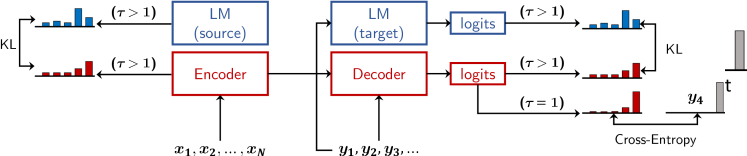
Figure 1: Targets with ls and lm-prior.

3.2 Relation to Label Smoothing

Label smoothing (ls) Szegedy et al. (2016) is a “trick” widely used in machine translation that also uses soft targets. Specifically, the target distribution at each step is the weighted average between the one-hot distribution $y_{k}$ of the ground-truth label and a uniform distribution over all other $K$ labels, parameterized by a smoothing parameter $\alpha$: $y_{i}^{\textsc{ls}}=y_{i}(1-\alpha)+\alpha/K$. The purpose of ls is to penalize confidence (i.e., low-entropy distributions).

We note that ls differs from the lm-prior in two ways. First, ls encourages the model to assign equal probability to all incorrect words Müller et al. (2019), which can be interpreted as a form of uninformative prior (Fig. 1). By contrast, the distributions of the lm are informative, because they express the beliefs of the lm at each step. Second, ls changes the target distribution (i.e., first term in Eq. (1)), whereas the lm-prior involves an additional term, hence the two methods are orthogonal.

language-pair	train	dev	test
English-Turkish	192,482	3,007	3,000
English-German	275,561	3,004	2,998

Table 1: Dataset statistics after preprocessing.

4 Experiments

Datasets

We use two low-resource language pairs (Table 1): the English-German (EN-DE) News Commentary v13 provided by WMT Bojar et al. (2018)  and the English-Turkish (EN-TR) WMT-2018 parallel data from the SETIMES2 corpus. We use the official WMT-2017 and 2018 test sets as the development and test set, respectively.

As monolingual data for English and German we use the News Crawls 2016 articles Bojar et al. (2016) and for Turkish we concatenate all the available News Crawls data from 2010-2018, which contain 3M sentences. For English and German we subsample 3M sentences to match the Turkish data, as well as 30M to measure the effect of stronger lms. We remove sentences longer than 50 words.

Pre-processing

We perform punctuation normalization and truecasing and remove pairs, in which either of the sentences has more than 60 words or length ratio over 1.5. The text is tokenized with sentencepiece (SPM; Kudo and Richardson (2018)) with the “unigram” model. For each language we learn a separate SPM model with 16K symbols, trained on its respective side of the parallel data. For English, we train SPM on the concatenation of the English-side of the training data from each dataset, in order to have a single English vocabulary and be able to re-use the same lm.

parameter	value
	tm	lm
Embedding size	512	1024
Transformer hidden size	1024	4096
Transformer layers	6	6
Transformer heads	8	16
Dropout (all)	0.3	0.3

Table 2: Hyperparameters of the tms and lms.

language	3M (ppl$\downarrow$)	30M (ppl$\downarrow$)
English	29.70	25.02
German	22.71	19.22
Turkish	22.78	–

Table 3: Perplexity scores for lms trained on each language’s monolingual data, computed on a small held-out validation set per language.

Model Configuration

In all experiments, we use the Transformer architecture for both the lms and tms. Table 2 lists all their hyperparameters. For the tms we found that constraining their capacity and applying strong regularization was crucial, otherwise they suffered from over-fitting. We also found that initializing all weights with glorot-uniform Glorot and Bengio (2010) initialization and using pre-norm residual connections Xiong et al. (2020); Nguyen and Salazar (2019), improved stability. We also tied the embedding and the output (projection) layers of the decoders Press and Wolf (2017); Inan et al. (2017).

We optimized our models with Adam Kingma and Ba (2015) with a learning rate of 0.0002 and a linear warmup for the first 8K steps, followed by inverted squared decay and with mini-batches with 5000 tokens per batch. We evaluated each model on the dev set every 5000 batches, by decoding using greedy sampling, and stopped training if the bleu score did not increase after 10 iterations.

For the lm training we followed the same optimization process as for the tms. However, we use Transformer-large configuration, in order to obtain a powerful lm-prior. Crucially, we did not apply ls during the lm pretraining, because, as discussed, it pushes the models to assign equal probability to all incorrect words Müller et al. (2019), which will make the prior less informative. In Table 3 we report the perplexities achieved by each lm on different scales of monolingual data.

We developed our models in PyTorch Paszke et al. (2019) and we used the Transformer implementation from JoeyNMT Kreutzer et al. (2019). We make our code publically available.

Method	DE$\rightarrow$EN		EN$\rightarrow$DE		TR$\rightarrow$EN		EN$\rightarrow$TR
	dev	test	dev	test	dev	test	dev	test
Base	$\text{22.6}\scriptscriptstyle\pm\text{0.1}$	$\text{26.9}\scriptscriptstyle\pm\text{0.1}$	$\text{18.3}\scriptscriptstyle\pm\text{0.3}$	$\text{25.6}\scriptscriptstyle\pm\text{0.2}$	$\text{15.9}\scriptscriptstyle\pm\text{0.0}$	$\text{16.6}\scriptscriptstyle\pm\text{0.3}$	$\text{12.2}\scriptscriptstyle\pm\text{0.1}$	$\text{11.2}\scriptscriptstyle\pm\text{0.2}$
Shallow-fusion	$\text{23.4}\scriptscriptstyle\pm\text{0.1}$	$\text{27.8}\scriptscriptstyle\pm\text{0.1}$	$\text{18.5}\scriptscriptstyle\pm\text{0.2}$	$\text{26.0}\scriptscriptstyle\pm\text{0.1}$	$\text{16.5}\scriptscriptstyle\pm\text{0.1}$	$\text{17.3}\scriptscriptstyle\pm\text{0.3}$	$\text{12.7}\scriptscriptstyle\pm\text{0.0}$	$\text{11.5}\scriptscriptstyle\pm\text{0.1}$
postnorm	$\text{20.4}\scriptscriptstyle\pm\text{0.2}$	$\text{24.5}\scriptscriptstyle\pm\text{0.3}$	$\text{16.6}\scriptscriptstyle\pm\text{0.1}$	$\text{22.9}\scriptscriptstyle\pm\text{0.3}$	$\text{13.8}\scriptscriptstyle\pm\text{0.2}$	$\text{14.8}\scriptscriptstyle\pm\text{0.1}$	$\text{11.0}\scriptscriptstyle\pm\text{0.1}$	$\text{10.2}\scriptscriptstyle\pm\text{0.2}$
postnorm+ ls	$\text{22.0}\scriptscriptstyle\pm\text{0.3}$	$\text{26.4}\scriptscriptstyle\pm\text{0.2}$	$\text{16.9}\scriptscriptstyle\pm\text{0.5}$	$\text{23.3}\scriptscriptstyle\pm\text{0.5}$	$\text{15.0}\scriptscriptstyle\pm\text{0.1}$	$\text{16.0}\scriptscriptstyle\pm\text{0.0}$	$\text{12.5}\scriptscriptstyle\pm\text{0.2}$	$\text{11.0}\scriptscriptstyle\pm\text{0.2}$
Base + ls	$\text{23.8}\scriptscriptstyle\pm\text{0.6}$	$\text{28.4}\scriptscriptstyle\pm\text{0.7}$	$\text{19.2}\scriptscriptstyle\pm\text{0.3}$	$\text{27.3}\scriptscriptstyle\pm\text{0.3}$	$\text{17.5}\scriptscriptstyle\pm\text{0.1}$	$\text{18.4}\scriptscriptstyle\pm\text{0.2}$	$\text{13.8}\scriptscriptstyle\pm\text{0.2}$	$\text{12.6}\scriptscriptstyle\pm\text{0.0}$
Base + Prior	$\textbf{24.9}\scriptscriptstyle\pm\text{0.0}$	$\textbf{30.2}\scriptscriptstyle\pm\text{0.1}$	$\textbf{20.5}\scriptscriptstyle\pm\text{0.3}$	$\textbf{29.1}\scriptscriptstyle\pm\text{0.7}$	$\textbf{18.5}\scriptscriptstyle\pm\text{0.2}$	$\textbf{19.5}\scriptscriptstyle\pm\text{0.2}$	$\textbf{15.1}\scriptscriptstyle\pm\text{0.1}$	$\textbf{13.8}\scriptscriptstyle\pm\text{0.1}$
Base + Prior + ls	$\text{\textul{25.1}}\scriptscriptstyle\pm\text{0.3}$	$\text{\textul{30.3}}\scriptscriptstyle\pm\text{0.3}$	$\text{\textul{20.8}}\scriptscriptstyle\pm\text{0.4}$	$\text{\textul{29.7}}\scriptscriptstyle\pm\text{0.7}$	$\text{18.5}\scriptscriptstyle\pm\text{0.3}$	$\text{19.5}\scriptscriptstyle\pm\text{0.2}$	$\text{\textul{15.5}}\scriptscriptstyle\pm\text{0.1}$	$\text{\textul{14.1}}\scriptscriptstyle\pm\text{0.2}$
Base + Prior (30M)	$\text{24.9}\scriptscriptstyle\pm\text{0.1}$	$\text{30.0}\scriptscriptstyle\pm\text{0.1}$	$\text{\textul{21.0}}\scriptscriptstyle\pm\text{0.4}$	$\text{\textul{29.8}}\scriptscriptstyle\pm\text{0.3}$	$\text{\textul{18.6}}\scriptscriptstyle\pm\text{0.0}$	$\text{19.5}\scriptscriptstyle\pm\text{0.2}$	–	–

Table 4: bleu scores of each model. Mean and stdev of 3 runs reported. The top section contains the main results, where all methods use lms trained on the same amount of data (3M). The bottom section compares different configurations of the lm-prior. Underlined scores denote gains over the “Base + Prior (3M)” model.

4.1 Experiments

We compare the proposed lm-prior with other approaches that incorporate a pretrained lm or regularize the outputs of the tm. First, we consider a vanilla nmt baseline without ls. Next, we compare with fusion techniques, namely shallow-fusion Gulcehre et al. (2015) and postnorm Stahlberg et al. (2018), which in the original paper outperformed other fusion methods. We also separately compare with label smoothing (ls), because it is another regularization method that uses soft targets. We report detokenized case-sensitive bleu using sacre-bleu Post (2018), and decode with beam search of size 5. The lms are fixed during training for both postnorm and the prior.

We tune the hyper-parameters of each method on the DE$\rightarrow$EN dev-set. We set the interpolation weight for shallow-fusion to $\beta$=0.1, the smoothing parameter for ls to $\alpha=0.1$. For the lm-prior we set the regularization weight to $\lambda$=0.5 and the temperature for $\mathcal{L}_{\textsc{kl}}$ to $\tau$=2.

4.2 Results

First, we use in all methods lms trained on the same amount of monolingual data, which is 3M sentences. We used the total amount of available Turkish monolingual data (3M) as the lowest common denominator. This is done to remove the effects of the size of monolingual data from the final performance of each method, across language-pairs and translation directions. The results are shown in the top section of Table 4. We also report results with recurrent neural networks (rnn) based on the attentional encoder-decoder Bahdanau et al. (2015) architecture in appendix A.

Overall, adding the lm-prior consistently improves performance in all experiments. Specifically, it yields up to +1.8 bleu score gains over the strongest baseline “Base+ls” (de$\rightarrow$en and en$\rightarrow$de). This shows that the proposed approach yields clear improvements, even with limited monolingual data (3M). As expected, ls proves to be very effective for mitigating over-fitting in such low-resource conditions. However, simply penalizing confidence helps up to a point, which is shown by the performance gap between “Base+ls” and “Base+prior”. We explore this further next (§ 5).

Shallow-fusion achieves consistent but marginal improvements in all language-pairs. It works by making small (local) changes to $p_{\textsc{tm}}$, which primarily helps improve fluency when the tm is very unsure about what to generate next. Surprisingly, when training the tm with the postnorm objective, it barely reaches the baseline. As we show in our analysis (§ 5), under postnorm the tm generates very sharp distributions, which is a result of how it combines $p_{\textsc{tm}}$ and $p_{\textsc{lm}}$. We identify two potential reasons for this result. First, in  Stahlberg et al. (2018) postnorm was only tested with ls, which to some extend hid the issue of low-entropy outputs. To verify this, we trained postnorm with ls. We observed that in this case, the scores improve significantly, but it still falls short in comparison with the other methods. Second, we note that the lms used in the original paper were also trained with ls. We hypothesize that by using an lm that emitted smoother distribution, it implicitly down-weighted the contribution of $p_{\textsc{lm}}$, that is similar to the small weight used in shallow-fusion, which works better in our experiments.

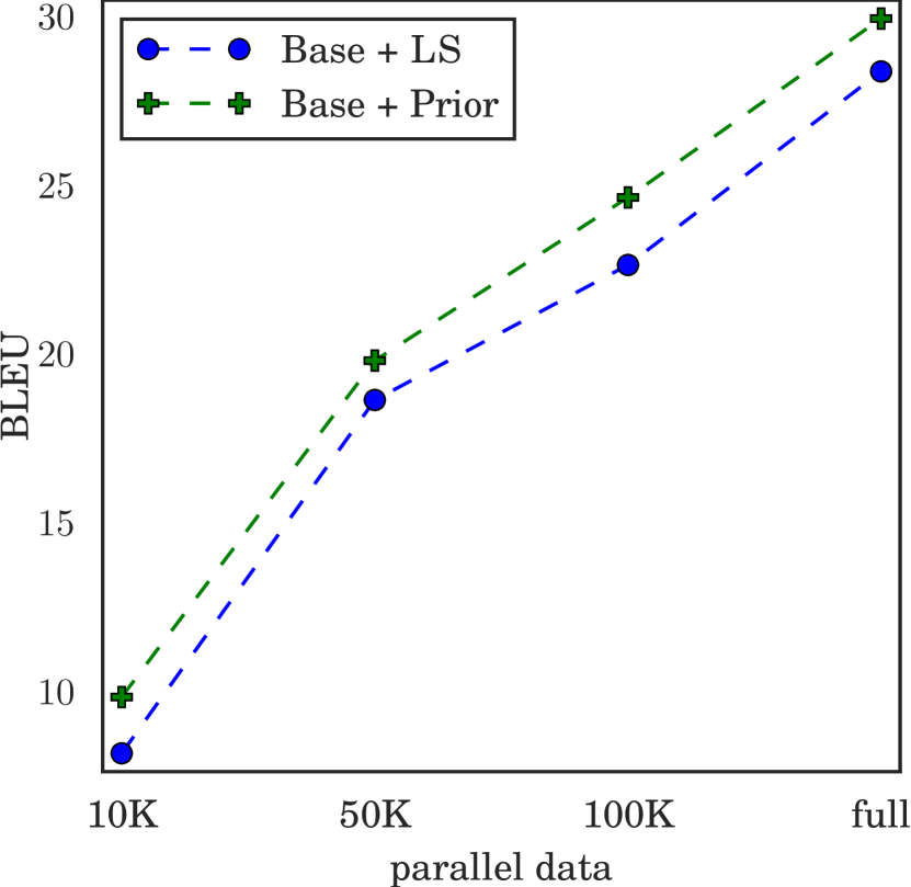
Figure 2: bleu scores (mean of 3 runs) on the de$\rightarrow$en test set with different scales of parallel data, using the lm trained on 30M English sentences.

Stronger lms

Next, we test how different variations of the lm-prior affect the translation quality (bottom section of Table 4). First, we lift the monolingual data constraint, in order to evaluate the impact of stronger lm-priors. Specifically, for English and German we use lms trained on 30M sentences. We observe that the stronger lms yield improvements only in the en$\rightarrow$de direction. This could partially be explained by the fact that German has richer morphology than English. Therefore, it is harder for the decoder to avoid grammatical mistakes in low-resource settings while translating into German, and a stronger prior is more helpful for x$\rightarrow$de than x$\rightarrow$en.

However, it is still surprising that the stronger English lm does not boost performance. We hypothesize that this might be related to the limited capacity of the tms we used. Specifically, in the kd literature it has been found that the student’s performance is affected by the difference between the capacities of the student and teacher networks Cho and Hariharan (2019); Zhou et al. (2020). In preliminary experiments we also used big lms pretrained on generic large-scale data, such as gpt-2 Radford et al. (2019), but we failed to achieve any measurable improvements over the baseline. Besides the discrepancy in the capacity between the lm and the tm, we suspect that another obstacle in this case is the large vocabulary size used in gpt-2 (50K symbols). In particular, Sennrich and Zhang (2019) showed that in low-resource nmt, using a very small vocabulary (2K-10K symbols) is the most important factor that affects translation performance. A potential solution could be to finetune gpt-2 on the small vocabulary of the tm Zhao et al. (2019) and then use it as a prior, but we leave this exploration for future work.

Prior + ls

We also evaluate a combination of the lm-prior with ls. We observe that in most experiments it has small but additive effects. This implicitly suggests that the two approaches are complementary to each other. ls smooths the one-hot target distribution, which penalizes confidence, whereas the lm-prior helps improve fluency. We further explore their differences in our analysis (§. 5), by showing the effects each method has on the tm’s distributions.

4.3 Extremely Low-Resource Experiments

We also conducted experiments that measure the effect of the lm-prior on different scales of parallel data. Specifically, we emulate more low-resource conditions, by training on subsets of the EN$\rightarrow$DE parallel data. In Fig. 2 we compare the bleu scores of the “Base+ls” and the “Base+Prior (30M)”.

Overall, we observe that adding the lm-prior yields consistent improvements, even with as little as 10K parallel sentences. The improvements have a weak correlation with the size of parallel data. We hypothesize that by exposing the tm to a larger sample of target-side sentences, it has the opportunity to extract more information from the prior. However, we anticipate that in more high-resource settings the improvements will start to diminish.

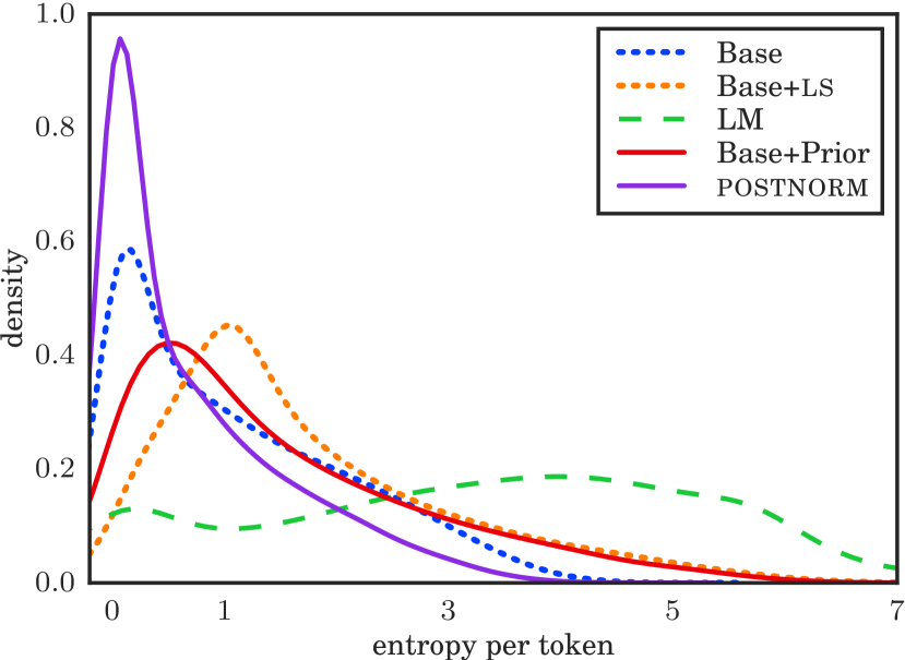
Figure 3: Estimated densities based on each model’s entropy on the de$\rightarrow$en test set.

5 Analysis

The main results show that ls, that simply penalizes confidence, is a very effective form of regularization in low-resource settings. We conduct a qualitative comparison to test whether the improvements from the proposed lm-prior are due to penalizing confidence, similar to ls, or from actually using information from the lm. Specifically, we evaluate each model on the de$\rightarrow$en test-set and for each target token we compute the entropy of each model’s distribution. In Fig. 3 we plot for each model the density over all its entropy values.

First, we observe that the un-regularized “Base” model generates very confident (low-entropy) distributions, which suggests that it overfits on the small parallel data. As expected, the ls regularization successfully makes the tm less confident and therefore more robust to over-fitting. For additional context, we plot the entropy density of the lm and observe that, unsurprisingly, it is the most uncertain, since it is unconditional.

Interestingly, the model trained with the lm-prior emits more confident distributions than the “Base+ls” model, although it also achieves significantly better performance. This clearly shows that the gains cannot be explained just from smoothing the distributions of the tm and suggests that the model indeed exploits information from the lm.

Next, we focus on the “Base+postnorm” model and observe that it generates the most confident predictions. Note that, this finding aligns with a similar analysis in the original paper, where it was shown that under postnorm the tm generates low-entropy distributions. However, even though this method might improve fluency, it can hurt translation quality in certain cases. As described in Sec. 3, by multiplying the two distributions, only a small subset of words will have non-zero probability in the final distribution. This means that when there are “disagreements” between the tm and lm this can lead to wrong predictions. We illustrate this with a concrete example in Fig. 4. Although the tm predicted the correct word, the multiplication with the lm distribution caused the model to finally make a wrong prediction. Also, the final distribution assigns a relatively high probability to a word (“more”), which is not among the top predictions of neither the lm or the tm. By contrast, the lm-prior does not change the tm’s predictions, and the model has the flexibility to deviate from the prior.

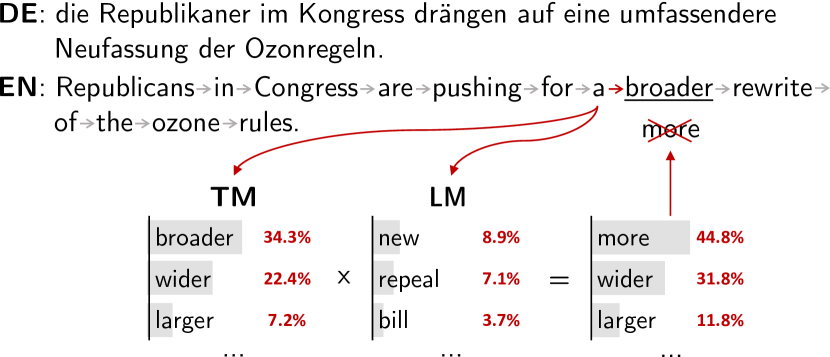
Figure 4: Example of failure of probability interpolation between lm and tm, while translating de$\rightarrow$en.

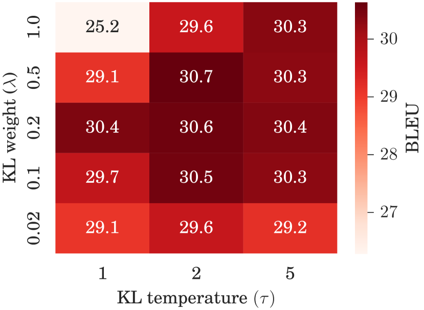
Figure 5: bleu scores on the DE-EN dev set of models trained with different $\lambda$ and $\tau$ for the $\mathcal{L}_{\textsc{kl}}$. Mean of 3 runs for each combination reported.

5.1 $\mathcal{L}_{\textsc{kl}}$ Sensitivity Analysis

The proposed regularization uses two different hyper-parameters in $\mathcal{L}_{\textsc{kl}}$, the weight $\lambda$ that controls the strength of the regularization, and the temperature $\tau$ that controls how much information from the long-tail of the lm to expose to the tm. We do a pairwise comparison between them, in order to measure how sensitive the model is to their values. In Fig. 5 we plot a heatmap of the bleu scores achieved by models trained on the DE$\rightarrow$EN dev-set with various combinations.

Overall, we observe a clear pattern emerging of how the lm-prior affects performance, which suggests that (1) using $\tau>1$ indeed helps the tm to acquire more of the knowledge encoded in the prior, and (2) increasing the strength of the regularization up to a point yields consistent improvements. We find that the performance is less sensitive to the value of $\tau$, compared to $\lambda$ and that by setting $\tau>1$, the model becomes also more robust to $\lambda$. Our explanation is that for $\tau>1$, the tm tries to match a larger part of the lm’s distribution and focuses less on its top-scoring words. Therefore, it is reasonable to observe that in the extreme case when we set equal weight to the $\mathcal{L}_{\textsc{mt}}$ and $\mathcal{L}_{\textsc{kl}}$ ($\lambda=1$) and $\tau=1$ the performance starts to degrade, because we strongly push the tm to match only the top-scoring predictions of the lm, that is unconditional. This forces the tm to pay less attention to the source sentence, which leads to translation errors.

6 Related Work

Most recent related work considers large pretrained models, either via transfer-learning or feature-fusion. Zhu et al. (2020); Clinchant et al. (2019); Imamura and Sumita (2019) explore combinations of using BERT as initialization for nmt, or adding BERT’s representations as extra features. Yang et al. (2019) address the problem of catastrophic-forgetting while transferring BERT in high-resource settings, with a sophisticated fine-tuning approach. In concurrent work, Chen et al. (2019) propose knowledge-distillation using BERT for various text generation tasks, including nmt, by incentivizing the sequence-to-sequence models to “look into the future”. However, in our work we address a different problem (low-resource nmt) and have different motivation. Also, we consider auto-regressive lms as priors, which have clear interpretation, unlike BERT that is not strictly a lm and requires bidirectional context. Note that, large pretrained lms, such as BERT or gpt-2, have not yet achieved the transformative results in nmt that we observe in natural language understanding tasks (e.g., GLUE benchmark Wang et al. (2019)).

There are also other approaches that have used posterior regularization to incorporate prior knowledge into nmt. Zhang et al. (2017) exploit linguistic real-valued features, such as dictionaries or length ratios, to construct the distribution for regularizing the tm’s posteriors. Recently, Ren et al. (2019) used posterior regularization for unsupervised nmt, by employing an smt model, which is robust to noisy data, as a prior over a neural tm to guide it in the iterative back-translation process. Finally, lms have been used in a similar fashion as priors over latent text sequences in discrete latent variable models Miao and Blunsom (2016); Havrylov and Titov (2017); Baziotis et al. (2019).

7 Conclusions

In this work, we present a simple approach for incorporating knowledge from monolingual data to nmt. Specifically, we use a lm trained on target-side monolingual data, to regularize the output distributions of a tm. This method is more efficient than alternative approaches that used pretrained lms, because it is not required during inference. Also, we avoid the translation errors introduced by lm-fusion, because the tm is able to deviate from the prior when needed.

We empirically show that while this method works by simply changing the training objective, it achieves better results than alternative lm-fusion techniques. Also, it yields consistent performance gains even with modest monolingual data (3M sentences) across all translation directions. This makes it useful for low-resource languages, where not only parallel but also monolingual data are scarce.

In future work, we intend to experiment with the lm-prior under more challenging conditions, such as when there is domain discrepancy between the parallel and monolingual data. Also, we would like to explore how to overcome the obstacles that prevent us from fully exploiting large pretrained lms (e.g., GPT-2) in low-resource settings.

Appendix A Appendix

Our preliminary experiments were conducted with recurrent neural networks (rnn), because we faced stability problems with the Transformer-based tms. We include those results here for completeness. The experiments were conducted with the 3M monolingual data in all translation directions, therefore they match the top section of the main results reported in the paper (Table 4). We observe the same relative performance as with the Transformer-based models, which verifies that the proposed approach transfers across architectures. However, the differences are smaller, because the rnn-based models achieved overall worse bleu scores and perplexities, for the translation and language modeling tasks, respectively.

parameter	value
	tm	lm
Embedding size (all)	256	512
Embedding dropout (all)	0.2	0.2
Encoder size	512	–
Encoder layers	2	–
Encoder dropout	0.2	–
Decoder size	512	1024
Decoder layers	2	2
Decoder dropout	0.2	0.2
Attention function	global	–

Table 5: Hyperparameters of rnn-based tms and lms.

Model Configuration

We employ the attentional encoder-decoder Bahdanau et al. (2015) architecture, using the “global” attention mechanism Luong et al. (2015). The recurrent cells are implemented using Long short-term memory (LSTM; Hochreiter and Schmidhuber (1997)) units. We use a bidirectional lstm encoder and a unidirectional lstm decoder. We also tie the embedding and the output (projection) layers of the decoders Press and Wolf (2017); Inan et al. (2017). and apply layer normalization Ba et al. (2016) to the last decoder representation, before the softmax.

We did not do any hyperparameter tuning, but selected the hyper-parameter values based on Sennrich and Zhang (2019), while also trying to keep approximately the same number of parameters as their Transformer-based counterparts. Table 5 lists all the model hyperparameters. All models were optimized with the Adam optimizer Kingma and Ba (2015) with a learning rate of 0.0002 and with mini-batches with 2000 tokens per batch.

Language Models

For the lms we used an identical architecture as the decoder of the tm, but with larger size. We also followed the same optimization process. Table 5 lists all the rnn-lm hyperparameters.

A.1 Language Models

For completeness, we include here some additional information about the training of the lms. In all experiments we paired the tm with lms with the same architecture, in order to evaluate how the proposed approach generalizes across architectures. We train one lm for each language, on its respective monolingual corpus. For the Transformer-based lms we also used a larger corpus for the high resource languages, as a part of our comparison shown in the main body of the paper. To evaluate the performance of the lms and to perform early stopping we used a small held-out development set with 10K sentences. Specifically, we stopped training when the perplexity on the development was not improved on for more than 10 epochs. In Table 6 we report the perplexities achieved by the lms on each monolingual corpus.

language	model	sentences (ppl$\downarrow$)
		3M	30M
English	LSTM	37.04	–
	Transformer (big)	29.70	25.02
German	LSTM	31.26	–
	Transformer (big)	22.71	19.22
Turkish	LSTM	31.26	–
	Transformer (big)	22.78	–

Table 6: Perplexity (ppl $\downarrow$) scores for lms trained on each language’s monolingual data, computed on a small held-out validation set per language.

Method	DE$\rightarrow$EN		EN$\rightarrow$DE		TR$\rightarrow$EN		EN$\rightarrow$TR
	dev	test	dev	test	dev	test	dev	test
Base	$\text{19.8}\scriptscriptstyle\pm\text{0.1}$	$\text{24.2}\scriptscriptstyle\pm\text{0.2}$	$\text{15.9}\scriptscriptstyle\pm\text{0.3}$	$\text{21.7}\scriptscriptstyle\pm\text{0.4}$	$\text{13.1}\scriptscriptstyle\pm\text{0.1}$	$\text{13.4}\scriptscriptstyle\pm\text{0.4}$	$\text{\,9.9}\scriptscriptstyle\pm\text{0.1}$	$\text{\,9.3}\scriptscriptstyle\pm\text{0.1}$
Shallow-fusion	$\text{20.3}\scriptscriptstyle\pm\text{0.1}$	$\text{24.9}\scriptscriptstyle\pm\text{0.3}$	$\text{16.0}\scriptscriptstyle\pm\text{0.5}$	$\text{22.1}\scriptscriptstyle\pm\text{0.6}$	$\text{13.5}\scriptscriptstyle\pm\text{0.2}$	$\text{13.8}\scriptscriptstyle\pm\text{0.5}$	$\text{10.2}\scriptscriptstyle\pm\text{0.2}$	$\text{\,9.7}\scriptscriptstyle\pm\text{0.1}$
postnorm	$\text{19.7}\scriptscriptstyle\pm\text{0.2}$	$\text{24.0}\scriptscriptstyle\pm\text{0.3}$	$\text{15.6}\scriptscriptstyle\pm\text{0.1}$	$\text{21.0}\scriptscriptstyle\pm\text{0.3}$	$\text{11.9}\scriptscriptstyle\pm\text{0.1}$	$\text{12.6}\scriptscriptstyle\pm\text{0.3}$	$\text{\,9.8}\scriptscriptstyle\pm\text{0.3}$	$\text{\,8.8}\scriptscriptstyle\pm\text{0.2}$
Base + LS	$\text{20.6}\scriptscriptstyle\pm\text{0.1}$	$\text{25.2}\scriptscriptstyle\pm\text{0.3}$	$\text{16.2}\scriptscriptstyle\pm\text{0.3}$	$\text{22.8}\scriptscriptstyle\pm\text{0.2}$	$\text{13.7}\scriptscriptstyle\pm\text{0.1}$	$\text{14.4}\scriptscriptstyle\pm\text{0.1}$	$\text{\textul{10.6}}\scriptscriptstyle\pm\text{0.1}$	$\text{\,9.8}\scriptscriptstyle\pm\text{0.2}$
Base + Prior	$\text{\textul{20.7}}\scriptscriptstyle\pm\text{0.3}$	$\text{\textul{25.3}}\scriptscriptstyle\pm\text{0.4}$	$\text{\textul{16.5}}\scriptscriptstyle\pm\text{0.4}$	$\text{\textul{23.0}}\scriptscriptstyle\pm\text{0.7}$	$\text{\textul{13.9}}\scriptscriptstyle\pm\text{0.1}$	$\text{\textul{14.5}}\scriptscriptstyle\pm\text{0.2}$	$\text{10.3}\scriptscriptstyle\pm\text{0.2}$	$\text{\textul{\,9.8}}\scriptscriptstyle\pm\text{0.1}$
Base + Prior + LS	$\text{{20.8}}\scriptscriptstyle\pm\text{0.2}$	$\text{{25.3}}\scriptscriptstyle\pm\text{0.3}$	$\text{{16.9}}\scriptscriptstyle\pm\text{0.3}$	$\text{{23.53}}\scriptscriptstyle\pm\text{0.2}$	$\text{{14.2}}\scriptscriptstyle\pm\text{0.2}$	$\text{{14.8}}\scriptscriptstyle\pm\text{0.1}$	$\text{{10.6}}\scriptscriptstyle\pm\text{0.2}$	$\text{{10.0}}\scriptscriptstyle\pm\text{0.2}$

Table 7: bleu scores of each rnn-nmt method. Mean and standard deviation of 3 runs reported.

References

- Ba and Caruana (2014) Jimmy Ba and Rich Caruana. 2014. Do deep nets really need to be deep? In Proceedings of the Advances in Neural Information Processing Systems, pages 2654–2662, Montreal, Quebec, Canada.
- Ba et al. (2016) Lei Jimmy Ba, Jamie Ryan Kiros, and Geoffrey E. Hinton. 2016. Layer normalization. arXiv preprint arXiv:1607.06450, abs/1607.06450.
- Bahdanau et al. (2015) Dzmitry Bahdanau, Kyunghyun Cho, and Yoshua Bengio. 2015. Neural machine translation by jointly learning to align and translate. In Proceedings of the International Conference on Learning Representations, San Diego, CA, USA.
- Baziotis et al. (2019) Christos Baziotis, Ion Androutsopoulos, Ioannis Konstas, and Alexandros Potamianos. 2019. SEQ^3: Differentiable sequence-to-sequence-to-sequence autoencoder for unsupervised abstractive sentence compression. In Proceedings of the Conference of the North American Chapter of the Association for Computational Linguistics: Human Language Technologies, pages 673–681, Minneapolis, Minnesota, USA. Association for Computational Linguistics.
- Bojar et al. (2016) Ondřej Bojar, Rajen Chatterjee, Christian Federmann, Yvette Graham, Barry Haddow, Matthias Huck, Antonio Jimeno Yepes, Philipp Koehn, Varvara Logacheva, Christof Monz, Matteo Negri, Aurélie Névéol, Mariana Neves, Martin Popel, Matt Post, Raphael Rubino, Carolina Scarton, Lucia Specia, Marco Turchi, Karin Verspoor, and Marcos Zampieri. 2016. Findings of the 2016 conference on machine translation. In Proceedings of the Conference on Machine Translation, pages 131–198, Berlin, Germany.
- Bojar et al. (2018) Ondřej Bojar, Christian Federmann, Mark Fishel, Yvette Graham, Barry Haddow, Philipp Koehn, and Christof Monz. 2018. Findings of the conference on machine translation (WMT). In Proceedings of the Conference on Machine Translation, pages 272–303, Belgium, Brussels.
- Brown et al. (1993) Peter F. Brown, Stephen A. Della Pietra, Vincent J. Della Pietra, and Robert L. Mercer. 1993. The mathematics of statistical machine translation: Parameter estimation. Computational Linguistics, 19(2):263–311.
- Bucila et al. (2006) Cristian Bucila, Rich Caruana, and Alexandru Niculescu-Mizil. 2006. Model compression. In Proceedings of the ACM SIGKDD International Conference on Knowledge Discovery and Data Mining, pages 535–541, Philadelphia, PA, USA.
- Chen et al. (2019) Yen-Chun Chen, Zhe Gan, Yu Cheng, Jingzhou Liu, and Jingjing Liu. 2019. Distilling the knowledge of bert for text generation. arXiv preprint arXiv:1911.03829.
- Cho and Hariharan (2019) Jang Hyun Cho and Bharath Hariharan. 2019. On the efficacy of knowledge distillation. In Proceedings of the IEEE International Conference on Computer Vision, pages 4794–4802.
- Clinchant et al. (2019) Stephane Clinchant, Kweon Woo Jung, and Vassilina Nikoulina. 2019. On the use of BERT for neural machine translation. In Proceedings of the Workshop on Neural Generation and Translation, pages 108–117, Stroudsburg, PA, USA.
- Devlin et al. (2019) Jacob Devlin, Ming-Wei Chang, Kenton Lee, and Kristina Toutanova. 2019. BERT: Pre-training of deep bidirectional transformers for language understanding. In Proceedings of the Conference of the North American Chapter of the Association for Computational Linguistics: Human Language Technologies, pages 4171–4186, Minneapolis, Minnesota.
- Domhan and Hieber (2017) Tobias Domhan and Felix Hieber. 2017. Using target-side monolingual data for neural machine translation through multi-task learning. In Proceedings of the Conference on Empirical Methods in Natural Language Processing, pages 1500–1505, Copenhagen, Denmark.
- Ganchev et al. (2010) Kuzman Ganchev, Jennifer Gillenwater, Ben Taskar, et al. 2010. Posterior regularization for structured latent variable models. Journal of Machine Learning Research, 11(Jul):2001–2049.
- Glorot and Bengio (2010) Xavier Glorot and Yoshua Bengio. 2010. Understanding the difficulty of training deep feedforward neural networks. In Proceedings of the Thirteenth International Conference on Artificial Intelligence and Statistics, volume 9 of Proceedings of Machine Learning Research, pages 249–256, Chia Laguna Resort, Sardinia, Italy. PMLR.
- Gulcehre et al. (2015) Caglar Gulcehre, Orhan Firat, Kelvin Xu, Kyunghyun Cho, Loic Barrault, Huei-Chi Lin, Fethi Bougares, Holger Schwenk, and Yoshua Bengio. 2015. On using monolingual corpora in neural machine translation. arXiv preprint arXiv:1503.03535.
- Havrylov and Titov (2017) Serhii Havrylov and Ivan Titov. 2017. Emergence of language with multi-agent games: Learning to communicate with sequences of symbols. In I. Guyon, U. V. Luxburg, S. Bengio, H. Wallach, R. Fergus, S. Vishwanathan, and R. Garnett, editors, Proceedings of the Advances in Neural Information Processing Systems, pages 2149–2159.
- Hinton et al. (2015) Geoffrey E. Hinton, Oriol Vinyals, and Jeffrey Dean. 2015. Distilling the knowledge in a neural network. arXiv preprint arXiv:1503.02531, abs/1503.02531.
- Hoang et al. (2018) Vu Cong Duy Hoang, Philipp Koehn, Gholamreza Haffari, and Trevor Cohn. 2018. Iterative back-translation for neural machine translation. In Proceedings of the Workshop on Neural Machine Translation and Generation, pages 18–24, Melbourne, Australia.
- Hochreiter and Schmidhuber (1997) Sepp Hochreiter and Jürgen Schmidhuber. 1997. Long short-term memory. Neural Computation, 9(8):1735–1780.
- Imamura and Sumita (2019) Kenji Imamura and Eiichiro Sumita. 2019. Recycling a pre-trained BERT encoder for neural machine translation. In Proceedings of the 3rd Workshop on Neural Generation and Translation, pages 23–31, Stroudsburg, PA, USA. Association for Computational Linguistics.
- Inan et al. (2017) Hakan Inan, Khashayar Khosravi, and Richard Socher. 2017. Tying word vectors and word classifiers: A loss framework for language modeling. In Proceedings of the International Conference on Learning Representations, Toulon, France.
- Kim and Rush (2016) Yoon Kim and Alexander M. Rush. 2016. Sequence-level knowledge distillation. In Proceedings of the Conference on Empirical Methods in Natural Language Processing, pages 1317–1327, Austin, Texas, USA.
- Kingma and Ba (2015) Diederik P. Kingma and Jimmy Ba. 2015. Adam: A method for stochastic optimization. In Proceedings of the International Conference on Learning Representations, San Diego, CA, USA.
- Koehn (2010) Philipp Koehn. 2010. Statistical Machine Translation, 1st edition. Cambridge University Press, New York, NY, USA.
- Koehn and Knowles (2017) Philipp Koehn and Rebecca Knowles. 2017. Six challenges for neural machine translation. In Proceedings of the Workshop on Neural Machine Translation, pages 28–39, Vancouver, Canada.
- Kreutzer et al. (2019) Julia Kreutzer, Joost Bastings, and Stefan Riezler. 2019. Joey NMT: A minimalist NMT toolkit for novices. To Appear in EMNLP-IJCNLP 2019: System Demonstrations.
- Kudo and Richardson (2018) Taku Kudo and John Richardson. 2018. SentencePiece: A simple and language independent subword tokenizer and detokenizer for neural text processing. In Proceedings of the Conference on Empirical Methods in Natural Language Processing, pages 66–71, Brussels, Belgium.
- Luong et al. (2015) Thang Luong, Hieu Pham, and Christopher D. Manning. 2015. Effective approaches to attention-based neural machine translation. In Proceedings of the Conference on Empirical Methods in Natural Language Processing, pages 1412–1421, Lisbon, Portugal.
- Miao and Blunsom (2016) Yishu Miao and Phil Blunsom. 2016. Language as a Latent Variable: Discrete Generative Models for Sentence Compression. In Proceedings of the Conference on Empirical Methods in Natural Language Processing, pages 319–328, Austin, Texas.
- Mikolov et al. (2011) Tomas Mikolov, Stefan Kombrink, Anoop Deoras, Lukar Burget, and Jan Cernocky. 2011. Rnnlm-recurrent neural network language modeling toolkit. In Proceedings of the ASRU Workshop, pages 196–201.
- Müller et al. (2019) Rafael Müller, Simon Kornblith, and Geoffrey E Hinton. 2019. When does label smoothing help? pages 4696–4705.
- Nguyen and Salazar (2019) Toan Q. Nguyen and Julian Salazar. 2019. Transformers without tears: Improving the normalization of self-attention.
- Paszke et al. (2019) Adam Paszke, Sam Gross, Francisco Massa, Adam Lerer, James Bradbury, Gregory Chanan, Trevor Killeen, Zeming Lin, Natalia Gimelshein, Luca Antiga, Alban Desmaison, Andreas Kopf, Edward Yang, Zachary DeVito, Martin Raison, Alykhan Tejani, Sasank Chilamkurthy, Benoit Steiner, Lu Fang, Junjie Bai, and Soumith Chintala. 2019. Pytorch: An imperative style, high-performance deep learning library. In H. Wallach, H. Larochelle, A. Beygelzimer, F. d'Alché-Buc, E. Fox, and R. Garnett, editors, Proceedings of the Advances in Neural Information Processing Systems, pages 8024–8035.
- Post (2018) Matt Post. 2018. A call for clarity in reporting BLEU scores. In Proceedings of the Conference on Machine Translation, pages 186–191, Brussels, Belgium.
- Press and Wolf (2017) Ofir Press and Lior Wolf. 2017. Using the output embedding to improve language models. In Proceedings of the Conference of the European Chapter of the Association for Computational Linguistics, pages 157–163, Valencia, Spain.
- Radford et al. (2019) Alec Radford, Jeff Wu, Rewon Child, David Luan, Dario Amodei, and Ilya Sutskever. 2019. Language models are unsupervised multitask learners.
- Ramachandran et al. (2017) Prajit Ramachandran, Peter Liu, and Quoc Le. 2017. Unsupervised pretraining for sequence to sequence learning. In Proceedings of the Conference on Empirical Methods in Natural Language Processing, pages 383–391, Copenhagen, Denmark.
- Ren et al. (2019) Shuo Ren, Zhirui Zhang, Shujie Liu, Ming Zhou, and Shuai Ma. 2019. Unsupervised neural machine translation with smt as posterior regularization. In Proceedings of the AAAI Conference on Artificial Intelligence, volume 33, pages 241–248.
- Sennrich et al. (2016) Rico Sennrich, Barry Haddow, and Alexandra Birch. 2016. Improving neural machine translation models with monolingual data. In Proceedings of the Annual Meeting of the Association for Computational Linguistics, pages 86–96, Berlin, Germany.
- Sennrich and Zhang (2019) Rico Sennrich and Biao Zhang. 2019. Revisiting low-resource neural machine translation: A case study. In Proceedings of the Annual Meeting of the Association for Computational Linguistics, pages 211–221, Florence, Italy.
- Shannon and Weaver (1949) Claude E Shannon and Warren Weaver. 1949. The mathematical theory of communication. Urbana, 117.
- Skorokhodov et al. (2018) Ivan Skorokhodov, Anton Rykachevskiy, Dmitry Emelyanenko, Sergey Slotin, and Anton Ponkratov. 2018. Semi-supervised neural machine translation with language models. In Proceedings of the AMTA Workshop on Technologies for MT of Low Resource Languages, pages 37–44, Boston, MA. Association for Machine Translation in the Americas.
- Sriram et al. (2018) Anuroop Sriram, Heewoo Jun, Sanjeev Satheesh, and Adam Coates. 2018. Cold fusion: Training seq2seq models together with language models. In Proceedings of Interspeech, pages 387–391.
- Stahlberg et al. (2018) Felix Stahlberg, James Cross, and Veselin Stoyanov. 2018. Simple fusion: Return of the language model. In Proceedings of the Conference on Machine Translation, pages 204–211, Belgium, Brussels.
- Sutskever et al. (2014) Ilya Sutskever, Oriol Vinyals, and Quoc V Le. 2014. Sequence to sequence learning with neural networks. In Advances in neural information processing systems, pages 3104–3112.
- Szegedy et al. (2016) Christian Szegedy, Vincent Vanhoucke, Sergey Ioffe, Jon Shlens, and Zbigniew Wojna. 2016. Rethinking the inception architecture for computer vision. In Proceedings of the IEEE conference on computer vision and pattern recognition, pages 2818–2826.
- Vaswani et al. (2017) Ashish Vaswani, Noam Shazeer, Niki Parmar, Jakob Uszkoreit, Llion Jones, Aidan N Gomez, Łukasz Kaiser, and Illia Polosukhin. 2017. Attention is all you need. In Proceedings of the Advances in Neural Information Processing Systems, pages 5998–6008, Long Beach, CA, USA.
- Wang et al. (2019) Alex Wang, Amanpreet Singh, Julian Michael, Felix Hill, Omer Levy, and Samuel R. Bowman. 2019. GLUE: A multi-task benchmark and analysis platform for natural language understanding. In International Conference on Learning Representations.
- Xiong et al. (2020) Ruibin Xiong, Yunchang Yang, Di He, Kai Zheng, Shuxin Zheng, Huishuai Zhang, Yanyan Lan, Liwei Wang, and Tie-Yan Liu. 2020. On layer normalization in the transformer architecture.
- Yang et al. (2019) Jiacheng Yang, Mingxuan Wang, Hao Zhou, Chengqi Zhao, Yong Yu, Weinan Zhang, and Lei Li. 2019. Towards making the most of BERT in neural machine translation.
- Yee et al. (2019) Kyra Yee, Yann Dauphin, and Michael Auli. 2019. Simple and effective noisy channel modeling for neural machine translation. In Proceedings of the Conference on Empirical Methods in Natural Language Processing and the International Joint Conference on Natural Language Processing, pages 5700–5705, Hong Kong, China.
- Yu et al. (2017) Lei Yu, Phil Blunsom, Chris Dyer, Edward Grefenstette, and Tomás Kociský. 2017. The neural noisy channel.
- Yu et al. (2019) Lei Yu, Laurent Sartran, Wojciech Stokowiec, Wang Ling, Lingpeng Kong, Phil Blunsom, and Chris Dyer. 2019. Putting machine translation in context with the noisy channel model.
- Zhang et al. (2017) Jiacheng Zhang, Yang Liu, Huanbo Luan, Jingfang Xu, and Maosong Sun. 2017. Prior knowledge integration for neural machine translation using posterior regularization. In Proceedings of the Annual Meeting of the Association for Computational Linguistics, pages 1514–1523, Vancouver, Canada.
- Zhao et al. (2019) Sanqiang Zhao, Raghav Gupta, Yang Song, and Denny Zhou. 2019. Extreme language model compression with optimal subwords and shared projections.
- Zhou et al. (2020) Chunting Zhou, Jiatao Gu, and Graham Neubig. 2020. Understanding knowledge distillation in non-autoregressive machine translation. In International Conference on Learning Representations.
- Zhu et al. (2020) Jinhua Zhu, Yingce Xia, Lijun Wu, Di He, Tao Qin, Wengang Zhou, Houqiang Li, and Tieyan Liu. 2020. Incorporating bert into neural machine translation. In International Conference on Learning Representations.