KUNS-2815

Implications of the weak gravity conjecture
in anomalous quiver gauge theories

Yoshihiko Abe¹ , Tetsutaro Higaki² and Rei Takahashi²

¹Department of Physics, Kyoto University, Kyoto 606-8502, Japan
²Department of Physics, Keio University, Yokohama 223-8533, Japan

1 Introduction

Swampland conjectures attract much attention recently in various apsects [1, 2, 3, 4, 5, 6, 7]. The conjectures are expected to constrain effective field theories to be consistent with quantum gravity, and give us new insights into not only the string theory as a candidate of quantum gravity but also physics beyond the Standard Model (SM).

Among them, the weak gravity conjecture (WGC) requires theories consistent with quantum gravity to include a charged state with a charge $q$ and a mass $m$ satisfying the weak gravity bound [3],

$$eq\geq\frac{m}{\sqrt{2}M_{\mathrm{Pl}}},$$ (1)

so that an extremal black holes can have a decay channel. The WGC briefly states that the gravity is the weakest force. Here, $e$ is an anomaly-free gauge coupling and $M_{\mathrm{Pl}}$ is the reduced Planck mass. The WGC can be extended to theories with multiple $U(1)$ groups [8] and also to a scalar exchange force such as a Yukawa interaction [9, 10, 11, 12, 13]. The latter extension is called the scalar weak gravity conjecture (SWGC) . These conjectures also have been checked in several aspects [14, 15], and indicate that repulsive forces of gauge interactions among the same species of particles are stronger than attractive forces of gravity and Yukawa interactions among them [16].

The situation may not be so simple in chiral gauge theories. IR symmetries are often obtained through the breaking of UV symmetries, and an IR gauge coupling is given by a linear combination of UV gauge couplings as in the SM. The linear combinations are determined by the Stückelberg couplings among the gauge bosons and would-be Nambu-Goldstone bosons (or axions) associated with the symmetry breaking. This is applicable not only to anomaly-free gauge theories but also to consistent theories possessing anomalous $U(1)$ gauge groups. In theories with an anomalous $U(1)$, an axion field plays an important role to cancel the gauge anomalies: the gauge invariance is (non-linearly) restored owing to the axion coupling to topological terms of the gauge fields on top of the Stückelberg couplings. As in the ordinary spontaneous symmetry breaking, these Stückelberg couplings lead to the gauge boson mass and determine the eigenstate of massless gauge boson. Thus the gauge boson of anomalous $U(1)$ symmetry is decoupled in the low energy limit. In the string theory, this anomaly cancellation is realized by the Green-Schwarz mechanism [18] involving string theoretic axions. 4D string models with anomalous $U(1)$’s have been well-discussed for realizing the SM [19, 20, 21, 22, 23, 24].

In this paper, we will focus on models with multiple $U(1)$ symmetries and chiral fermions. For models with $U(1)^{k}$, an anomaly-free $U(1)$ is given by a linear combination of the original symmetries:

$$U(1)_{\text{anomaly-free}}=\sum_{i=1}^{k}c_{i}U(1)_{i},$$ (2)

where $k$ is the number of $U(1)$ symmetries, $c_{i}~{}(i=1,2,\ldots,k)$ is a model-dependent ${\mathcal{O}}(1)$ coefficient and $U(1)_{i}$ is the $i$-th gauge group. We will discuss some examples in the following section. Then, the corresponding anomaly-free gauge coupling $e$ is given by

$$\frac{1}{e^{2}}=\sum_{i=1}^{k}\frac{c_{i}^{2}}{g_{i}^{2}},$$ (3)

where $g_{i}$ is the gauge coupling of the $U(1)_{i}$ symmetry. The gauge coupling $e$ will become necessarily very weak and smaller than the original coupling $g_{i}$ as the number of $U(1)$ gauge groups increases in the large $k$ limit. Thus, the WGC condition in Eq. (1) looks hard to be satisfied with an assumption that chiral anomlies can be canceled. In other words, the repulsive force among particles will then become very weak. It is conjectured that a certain class of chiral gauge theories with too many $U(1)$ symmetries can be in the swampland. It is noted that the gauge groups in 10D superstring theories are restricted [26], while those in 4D brane models seem less-constrained in the view point of tadpole condition. When magnitude of all the gauge couplings is comparable to each other, the Eq. (3) is rewitten as

$$eq\sim\frac{\tilde{g}}{\sqrt{k}}q\gtrsim\frac{m}{M_{\mathrm{Pl}}},$$ (4)

where $\tilde{g}\sim g_{i}$ for $\forall~{}i$ is the average of the gauge couplings. We find that the gauge coupling is scaling as $e\sim k^{-1/2}$ for a large $k$ and there exists an upper bound on $k$, $k\lesssim(q{\tilde{g}}\frac{M_{\mathrm{Pl}}}{m})^{2}$, if the WGC is correct and the mass $m$ remains non-zero in the large $k$ limit. This upper bound on $k$ is similar to the species bound [27], but $k$ is not the number of species but the number of $U(1)$ gauge groups in our case. Similar conditions for theories with a discrete $\mathbb{Z}_{k}$ (gauge) symmetry are also discussed in Refs. [28, 29]. Eq. (4) could be regarded as an example of the weak coupling conjecture [29].

A notion of quiver gauge theory is often used for theories in the presence of multiple gauge groups and bi-fundamental chiral fermions, and matches model building involving D-branes well [30, 31, 32, 33, 34, 35, 36, 37, 38, 39, 40]. Instead of concrete string models, in this paper we will consider quiver gauge theories with $U(1)^{k}$ gauge groups and focus on the anomaly-free gauge groups and the (S)WGC in a bottom-up approach, supposing that the remaining anomalies are canceled and then the anomalous gauge bosons get massive. In general, computation of anomalies depends on the matter content in models. In order to check anomaly-free $U(1)$’s systematically and study concretely the (S)WGC constraints on the gauge couplings, we restrict ourselves to several types of models controlled by discrete symmetries. However, a behavior of the anomaly-free gauge coupling in Eq. (3) does not change in general models with anomalous $U(1)$’s. The (S)WGC can constrain range of free parameters in low energy theories and show what parameter values are favored by UV theory in the view point of IR physics. In some quiver gauge theories of our interest, there exist a discrete symmetry associated with cyclic permutations between the gauge groups in certain quiver gauge theories, and the symmetry can generally be broken in anomaly-free $U(1)$ theories by a linear combination of $U(1)$’s as in Eq. (3). Some of quiver gauge theories remind us of deconstructed extra dimension [41, 42], which could relate our approach to the weak coupling conjecture in holography [29]. Also new insights can be given to chiral abelian gauge theories which may be a candidate of hidden sectors of dark matter models in particle physics [43].

This paper is organized as follows. In Sec. 2, we give a brief review of the (S)WGC and anomalous $U(1)$ symmetries. In Sec. 3, we will discuss concrete quiver gauge theories with $U(1)^{k}$, then identify the anomaly-free $U(1)$ symmetries. In Sec. 4, we numerically show the SWGC constraint on the gauge couplings and Yukawa couplings in a $U(1)^{4}$ quiver gauge theory. We discuss also a toy model from 5D orbifold compactification similarly. Sec. 5 is devoted to summary and conclusion. In this paper, we will discuss the above arguments with the tree level parameters.

2 Brief reviews of the (S)WGC and anomalous $U(1)$’s

2.1 The WGC and the SWGC

In this subsection, we give a brief review of the WGC and the SWGC in four dimension. The WGC claims that there exists a state with a charge $q$ and a mass $m$ satisfying the inequality

$$eq\geq\frac{m}{\sqrt{2}M_{\mathrm{Pl}}}$$ (5)

in a theory consistent with quantum gravity [3]. The factor of $1/\sqrt{2}$ comes from the relative normalization of the Newton force against the Coulomb one, and a generalization to an arbitrary dimension is straightforward [44]. This conjecture makes (super)extremal black holes decay into lighter ones.

The WGC can be extended to theories including a scalar exchange force such as a Yukawa interaction. This is called the SWGC [9, 10, 14]. Let us consider a theory with multiple $U(1)$ gauge groups:

$$S_{\mathrm{EM}}=\int d^{4}x\,\sqrt{-g}\biggl{[}\frac{M_{\mathrm{Pl}}^{2}}{2}\mathcal{R}-\sum_{a,b}\frac{1}{2}K_{ab}\partial_{\mu}\phi^{a}\partial^{\mu}\phi^{b}-\frac{1}{4}\sum_{i,j}f_{ij}(\phi)F^{(i)}_{\mu\nu}F^{(j)\mu\nu}\biggr{]}$$ (6)

where $\mathcal{R}$ is a Ricci scalar, $\phi^{a}$ is a real scalar field, $F^{(i)}_{\mu\nu}$ is a field strength of $U(1)_{i}$, $K_{ab}$ is a scalar kinetic matrix, $f_{ij}$ is a gauge kinetic function, and $i,~{}j~{}(=1,2,\ldots,k)$ and $a,~{}b$ denote the labels of $U(1)$ gauge groups and those of scalar fields respectively. The diagonal parts of $f_{ij}$ give the gauge couplings of $U(1)_{i}$’s and the off-diagonal components are kinetic mixings. The matter part action is given by

$$S_{\mathrm{matter}}=\int d^{4}x\,\sqrt{-g}\biggl{[}-\frac{1}{2}\sum_{a,b}K_{ab}\partial_{\mu}\Phi^{a}\partial^{\mu}\Phi^{b}+\overline{\psi}i\gamma^{\mu}\Bigl{(}\nabla_{\mu}+i\sum_{j}q_{j}A^{(j)}_{\mu}\Bigr{)}\psi-m(\Phi)\overline{\psi}\psi\biggr{]}$$ (7)

where $\psi$ is a Dirac spinor of a test particle for the SWGC and has a charge $q_{i}$ under the gauge group $U(1)_{i}$ and a mass $m(\Phi)$, and $\Phi^{a}$ is a real scalar field which may be different from $\phi^{a}$ in general. Here, the covariant derivative $\nabla_{\mu}$ includes the spin connection. The $\Phi^{a}$ is decomposed as

$$\Phi^{a}=\overline{\varphi}^{a}+\varphi^{a},$$ (8)

where $\overline{\varphi}^{a}$ is the background configuration of $\Phi^{a}$ and $\varphi^{a}$ denotes a fluctuation around the background. With these, the mass $m(\Phi)$ is rewritten as

$$m(\Phi)=m(\overline{\varphi})+\frac{\partial m}{\partial\varphi^{a}}\varphi^{a}+\cdots.$$ (9)

$m(\overline{\varphi})$ is the mass of the $\psi$ in the background $\overline{\varphi}^{a}$, and the higher order terms of $\varphi^{a}$ give the interaction terms between $\varphi^{a}$’s and $\psi$. Thus the Yukawa coupling reads:

$$S_{\mathrm{matter}}\supset\int d^{4}x\,\sqrt{-g}\,\sum_{a}y_{a}(\overline{\varphi})\varphi^{a}\overline{\psi}\psi,$$ (10)

$$y_{a}(\overline{\varphi}):=\frac{\partial m}{\partial\varphi^{a}}(\overline{\varphi})=\partial_{a}m(\overline{\varphi}).$$ (11)

Then the SWGC for $\psi$ is given by

$$\sum_{i,j}f^{ij}q_{i}q_{j}\geq\frac{m^{2}}{2M_{\mathrm{Pl}}^{2}}+\sum_{a,b}K^{ab}y_{a}y_{b},$$ (12)

where $f^{ij}$ and $K^{ab}$ are the inverse matrix of the $f_{ij}$ and $K_{ab}$ respectively. This inequality can be interpreted as the total gauge repulsive force is stronger than the sum of the attractive forces of the gravity and the total Yukawa interactions when we focus on forces acting between the test particle $\psi$: $|\vec{F}_{\mathrm{Coulomb}}|\geq|\vec{F}_{\mathrm{gravity}}|+|\vec{F}_{\mathrm{Yukawa}}|$. The absolute value of long-range force mediated by massless fields in four dimension is expressed as

$$|\vec{F}|=\frac{A}{4\pi r^{2}},$$ (13)

where a numerator $A$ is the factor corresponding to each force:

$$A_{\mathrm{Coulomb}}=\sum_{i,j}f^{ij}q_{i}q_{j},\quad A_{\mathrm{gravity}}=\frac{m^{2}}{2M_{\mathrm{Pl}}^{2}},\quad A_{\mathrm{Yukawa}}=\sum_{a,b}K^{ab}y_{a}y_{b}$$ (14)

If the scalars $\varphi^{a}$ are heavy, Yukawa interactions are short-range forces and neglected. Then the SWGC gets back to the WGC.

2.2 Anomalous $U(1)$ symmetries

In this subsection, we review cancellation of chiral $U(1)$ gauge anomalies by axion fields. In 4D effective field theories, gauge transformation of the axions can cancel the chiral anomalies produced by light chiral fermions in the presence of topological terms of the gauge fields and the Stückelberg couplings. In field theories with an anomaly-free $U(1)$ gauge symmetry, such axions are would-be Nambu-Goldstone bosons associated with the spontaneous breaking of the $U(1)$ symmetry. After integrating out heavy fermions with chiral $U(1)$ charges, we can obtain anomalous $U(1)$ in the low energy limit [45, 17]. In 4D string models, anomalies can be canceled by the Green-Schwarz mechanism involving string theoretic axions that originate from tensor fields, when tadpoles of brane charges are canceled [46, 47].

We shall consider the 4D action involving axions in addition to chiral fermions leading to chiral anomalies:

$$S_{\mathrm{axion}}=\sum_{i\in U(1)_{\mathrm{anomaly}}}\int d^{4}x\biggl{[}-\frac{1}{2}\frac{m_{i}^{2}}{g_{i}^{2}}\biggl{(}\sum_{I\in\mathrm{axions}}B_{iI}\partial_{\mu}\theta_{I}+A_{\mu}^{(i)}\biggr{)}^{2}+\sum_{I\in\mathrm{axions}}\frac{C_{iI}\theta_{I}}{32\pi^{2}}\epsilon^{\mu\nu\rho\sigma}F_{\mu\nu}^{(i)}F_{\rho\sigma}^{(i)}\biggr{]}.$$ (15)

Here, $\theta_{I}$ is an axion, $B_{iI}$ and $C_{iI}$ are constants, $m_{i}$ is the gauge boson mass. For the anomalous $U(1)$ symmetries, the fields transform as

$$\theta_{I}\to\theta_{I}-D_{Ii}\Lambda_{i},\qquad A_{\mu}^{(i)}\to A_{\mu}^{(i)}+\partial_{\mu}\Lambda_{i},$$ (16)

where $\Lambda_{i}$ is the transformation parameter, and we assume that $D_{Ii}$ satisfies $\sum_{I}B_{iI}D_{Ij}=\delta_{ij}$. The theory is invariant in the presence of chiral anomalies produced by gauge transformations against chiral fermions:

$$S_{\mathrm{anomaly}}=\sum_{i\in U(1)_{\mathrm{anomaly}}}\int d^{4}x\bigg{[}\sum_{I\in\mathrm{axions}}\Lambda_{i}\frac{C_{iI}D_{Ii}}{32\pi^{2}}\epsilon^{\mu\nu\rho\sigma}F_{\mu\nu}^{(i)}F_{\rho\sigma}^{(i)}\bigg{]},$$ (17)

such that $\delta_{\Lambda}S_{\rm total}=S_{\rm anomaly}+\delta_{\Lambda}S_{\rm axion}=0$. Thus, in terms of axions the anomaly-free $U(1)$’s are determined such that the coefficients of $C_{iI}$’s are vanishing. 4D effective action from 5D theory is also discussed, for instance, in Refs. [48, 49]. The anomalous gauge bosons become massive as

$$-\frac{1}{2}\frac{m_{i}^{2}}{g_{i}^{2}}\bigl{(}B_{iI}\partial_{\mu}\theta_{I}+A_{\mu}^{(i)}\bigr{)}^{2}=:-\frac{1}{2}\frac{m_{i}^{2}}{g_{i}^{2}}\bigl{(}\tilde{A}_{\mu}^{(i)}\bigr{)}^{2},$$ (18)

after $\theta$’s are eaten by them as in spontaneous gauge symmetry breaking. Further, for some non-anomalous gauge bosons, there can exist Stückelberg couplings

$$S_{\mathrm{axion}}=\sum_{i\in U(1)_{\text{non-anomalous}}}\int d^{4}x\bigg{[}-\frac{1}{2}\frac{m_{i}^{2}}{g_{i}^{2}}\bigg{(}\sum_{I\in\mathrm{axions}}B^{\prime}_{iI}\partial_{\mu}\theta_{I}+A_{\mu}^{{}^{\prime}(i)}\bigg{)}^{2}\bigg{]}.$$ (19)

The non-anomalous gauge bosons can become massive as the anomalous ones. Then, the repulsive forces mediated by such massive gauge bosons will not contribute to the WGC.

Hereafter, we suppose that this mechanism works in the quiver gauge theories studied in this paper, and these terms are ignored otherwise stated.

3 Quiver gauge theories and the WGC

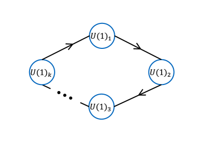
Figure 1: A quiver diagram with $k$ nodes.

In this section, we discuss quiver theories with $U(1)^{k}$ gauge symmetry and identify anomaly-free gauge groups. In general, computation of anomalies depends on the matter content in models. To check anomaly-free $U(1)$’s systematically and identify the gauge couplings concretely, we focus on several types of models controlled by discrete symmetries. However, an anomaly-free gauge coupling will be given by Eq. (3) in general cases. As for a quiver diagram in this paper, each node implies a gauge group whereas each arrow among two nodes shows a left-handed chiral fermion charged under two gauge groups. The number of arrows shows that of matters and a direction of an arrow is corresponding to the representation against two gauge groups. An arrowhead corresponds to anti-fundamental representation while its opposite side means fundamental one. For theories only with multiple $U(1)$ groups, (anti-)fundamental representation is supposed to have a charg e $+1$ ($-1$). A solid line shows a chiral (left-handed) fermion whereas a dashed line shows a complex scalar.

At first, we shall focus on non-supersymmetric gauge theories with bi-fundamental chiral fermions of $(\bm{N}_{1},\overline{\bm{N}_{2}})$ representation under $U(N_{1})\times U(N_{2})\times\cdots$ gauge group, which is inspired by D-brane models. Although there exist many types of quiver diagrams corresponding to gauge theories, for simplicity we focus on theories including only $U(1)$ groups in the diagrams such as Fig. 1. Since there exist chiral fermions, chiral gauge anomalies can generally be produced as a consequence. We study cancellation condition of chiral anomalies to identify anomaly-free gauge couplings at the tree level, and apply the couplings to the WGC. Anomaly-free conditions for $U(N)^{3}$ and $U(N)^{4}$ are discussed in Appendix A. For instance, in $SU(N)^{k}$ theories with a general $N$, non-abelian gauge anomaly cancellations require that the number of incoming arrows is equal to that of outgoing ones at each node. In $U(1)^{k}$ theories we will simply mimic $SU(N)^{k}$ cases because in D-brane models a gauge group can be given by $U(N)=U(1)\times SU(N)$ rather than just $SU(N)$, hence $U(1)$ and $SU(N)$ are considered simultaneously. We suppose that the anomalies are canceled as in Sec. 2.2 and then (non-)anomalous gauge fields get massive in a gauge invariant form. Quiver gauge theories associated with deconstructed extra dimension [41, 42] could relate our approach to the weak coupling conjecture [29].

In quiver gauge theories with $U(1)^{k}$ of our interest, the action is written by

$$S=\sum_{j=1}^{k}\int d^{4}x\biggl{[}-\frac{1}{4g_{j}^{2}}F^{(j)}_{\mu\nu}F^{(j)\mu\nu}+\overline{\psi}_{j,j+1}i\gamma^{\mu}\bigl{(}\partial_{\mu}+iA^{(j)}_{\mu}-iA^{(j+1)}_{\mu}\bigr{)}\psi_{j,j+1}+\cdots\biggr{]},$$ (20)

where ellipsis shows gravity and interaction terms among fermions which we have neglected. We assume that kinetic mixings among gauge fields are absent at the tree level for simplicity, and will ignore them in this paper. The gauge field of $U(1)_{j}$ is denoted by $A^{(j)}_{\mu}$ and $\psi_{j,j+1}$ is a left-handed spinor with a charge of $(+1,-1)$ against the $(U(1)_{j},U(1)_{j+1})$ gauge group as noted above. The index runs as $j=1,2,\ldots,k$ and satisfies $k+1\equiv 1$. There will exist a symmetry that shifts labels simultaneously as $j\to j+1$:

$$g_{j}\to g_{j+1},\quad A_{\mu}^{(j)}\to A_{\mu}^{(j+1)},\quad\psi_{j,j+1}\to\psi_{j+1,j+2},$$ (21)

when we treat the gauge couplings as spurion fields, which are expected to be moduli fields in the string theory. This can be regarded as a $\mathbb{Z}_{k}$ symmetry acting on $k$ nodes with a element of

$$\left(\begin{array}[]{cccccc}0&1&0&0&\cdots&0\\ 0&0&1&0&\cdots&0\\ 0&0&0&1&\cdots&0\\ &&&&\ddots&\\ 1&0&0&0&\cdots&0\end{array}\right).$$ (27)

We can study anomalies and identify anomaly-free $U(1)$’s systematically owing to this symmetry as seen below. This symmetry will be broken in the low energies when an anomaly-free gauge group is given by a linear combination of UV $U(1)$’s. So, interactions of axions to gauge fields are expected to violate this discrete symmetry.

In terms of particle phenomenology, this theory may be the hidden sector for dark matter apart from the visible sector [43]. In Appendix B, we discussed also several quiver models not shown in this section.

3.1 $U(1)^{2k-1}$

We consider quiver gauge theories with $U(1)^{2k-1}$ groups as shown in Fig. 1. These types of (supersymmetric) models have often been studied in D-brane models on orbifolds or intersecting/magnetized D-brane models. They are used also to realize realistic Yukawa couplings or higher order couplings. We hereafter focus just on fermions producing anomalies. As seen below, these theories can have an unique anomaly-free $U(1)$.

3.1.1 $U(1)^{3}$

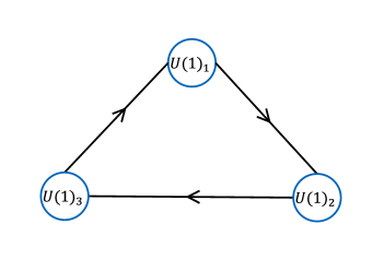
Figure 2: Three nodes quiver diagram.

One of the simplest case is the quiver gauge theory with $U(1)^{3}=U(1)_{1}\times U(1)_{2}\times U(1)_{3}$ groups in Fig. 2. As in Eq. (20), there exist three left-handed chiral fermions $\psi_{Li}~{}(i=1,2,3)$, which have charges of $(1,-1,0),~{}(0,1,-1)$ and $(-1,0,1)$ against $(U(1)_{1},U(1)_{2},U(1)_{3})$ respectively. This model will have a ${\mathbb{Z}}_{3}$ symmetry as noted above, and there is no other choices to connect each node. The divergences of $U(1)^{3}$ chiral currents $j^{i\mu}~{}(i=1,2,3)$ are given by

$$\begin{cases}\partial\cdot j^{1}=Q_{2}-Q_{3}\\ \partial\cdot j^{2}=Q_{3}-Q_{1}\\ \partial\cdot j^{3}=Q_{1}-Q_{2},\end{cases}$$ (28)

where $\partial\cdot j^{i}=\partial_{\mu}j^{i\mu}$ and $Q_{i}$ is the topological charge density, $Q_{i}=\frac{1}{32\pi^{2}}\epsilon^{\mu\nu\rho\sigma}F^{(i)}_{\mu\nu}F^{(i)}_{\rho\sigma}$. Thus we define the anomaly-free $U(1)$ by

$$U(1)_{X}:=c_{1}U(1)_{1}+c_{2}U(1)_{2}+c_{3}U(1)_{3},$$ (29)

and impose the divergence of its current to vanish

$$\partial\cdot j^{X}=\sum_{i=1,2,3}c_{i}\partial\cdot j^{i}=(-c_{2}+c_{3})Q_{1}+(c_{1}-c_{3})Q_{2}+(-c_{1}+c_{2})Q_{3}\equiv 0.$$ (30)

Then the solution is

$$U(1)_{X}=U(1)_{1}+U(1)_{2}+U(1)_{3}.$$ (31)

In this model, the anomaly-free gauge group is determined uniquely (up to overall normalization of the charges), and its gauge coupling is given by

$$\frac{1}{e_{X}^{2}}=\frac{1}{g_{1}^{2}}+\frac{1}{g_{2}^{2}}+\frac{1}{g_{3}^{2}}.$$ (32)

Here, the anomaly-free gauge coupling $e_{X}$ is written so that the gauge kinetic term becomes the canonical form:

$$-\sum_{j}\frac{1}{4g_{j}^{2}}F_{\mu\nu}^{(j)}F^{(j)\mu\nu}=-\frac{1}{4e_{X}^{2}}F_{\mu\nu}^{(X)}F^{(X)\mu\nu}+(\text{anomalous gauge fields}).$$ (33)

Thus, the anomaly-free gauge coupling $e_{X}$ can be smaller than the original $U(1)$ gauge couplings $g_{i}$’s.

It is noted that all the matters are then neutral under this anomaly-free $U(1)_{X}$, i.e., $\forall~{}q_{X}=0$. It seems that this model may not be naively applied to the WGC, but the presence of global symmetries is important. The low energy Lagrangian will be given by

$$\mathcal{L}=\sum_{i\in\text{ matter}}i\overline{\psi_{Li}}{\ooalign{\hfil/\hfil\crcr$\partial$}}\psi_{Li}-\frac{1}{4e_{X}^{2}}\bigl{(}F^{(X)}_{\mu\nu}\bigr{)}^{2}+\cdots,$$ (36)

if anomaly-free gauge boson $A_{\mu}^{(X)}$ survives in low energy limit. Ellipsis includes interactions among fermions and anomaly-free gauge boson and there will additionally exist kinetic mixings such as $K_{ij}\overline{\psi_{iL}}{\ooalign{\hfil/\hfil\crcr$\partial$}}\psi_{jL}$ and Majorana mass terms of $-M_{ij}\overline{\psi^{C}_{iL}}\psi_{jL}$ in low energy limit after anomalous massive bosons are integrated out. These terms will violate invariance under phase rotations of fermions. Now the original ${\mathbb{Z}}_{3}$ symmetry acts as $e_{X}\to e_{X},~{}A_{\mu}^{(X)}\to A_{\mu}^{(X)}$ and $\psi_{Li}\to\psi_{Li+1}$, but whether this low energy theory has the ${\mathbb{Z}}_{3}$ symmetry depends on parameters for fermions. Since all fermions are neutral under $U(1)_{X}$, global symmetries will be hard to survive in the low energy limit while discrete gauge symmetries originating from the anomalous $U(1)$’s can survive if any. If global symmetries survive, this model is in the swampland. It will be necessary to embed this model into string theory in order to know what kind of symmetries survives. This is beyond the scope of the paper and left for future work.

3.1.2 $U(1)^{2k-1}$

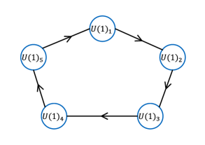
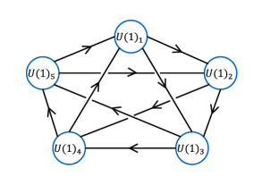
Figure 3: Quiver diagrams with five nodes. Both diagrams have a $\mathbb{Z}_{5}$ cyclic symmetry among each node. In the right diagram, all nodes are connected with arrows.

We consider quiver gauge theories with more general $U(1)^{2k-1}$ groups. Fig. 3 shows quiver diagrams with the five nodes, and it is noted that the number of incoming arrows is equal to that of outgoing ones at each node and both diagrams have a $\mathbb{Z}_{5}$ cyclic symmetry among each node. As in Eq. (20) and in the left diagram of Fig. 3, we have five left-handed fermions charged against $(U(1)_{1},U(1)_{2},U(1)_{3},U(1)_{4},U(1)_{5})$. The divergences of $U(1)^{5}$ chiral currents are given by

$$\partial\cdot\left(\begin{array}[]{c}j^{1}\\ j^{2}\\ j^{3}\\ j^{4}\\ j^{5}\end{array}\right)=\left(\begin{array}[]{ccccc}0&1&0&0&-1\\ -1&0&1&0&0\\ 0&-1&0&1&0\\ 0&0&-1&0&1\\ 1&0&0&-1&0\end{array}\right)\left(\begin{array}[]{c}Q_{1}\\ Q_{2}\\ Q_{3}\\ Q_{4}\\ Q_{5}\end{array}\right).$$ (52)

The number of anomaly-free $U(1)$’s is given by that of zero eigenvalues of this coefficient matrix, and we find only one zero eigenvalue in this model. The anomaly-free $U(1)$ is given by the corresponding eigenvector

$$U(1)_{\text{anomaly-free}}=U(1)_{1}+U(1)_{2}+U(1)_{3}+U(1)_{4}+U(1)_{5}.$$ (53)

Thus all matters are again neutral under this anomaly-free $U(1)$ and this system will not simply be applied to the WGC. The situation is similar to the three quivers model in Sec. 3.1.1.

The result is not changed by adding five chiral fermions to this model as in the right diagram of Fig. 3. Then their action is additionally given by

$$S=\sum_{j=1}^{5}\int d^{4}x\biggl{[}\overline{\psi}_{j,j+2}i\gamma^{\mu}\bigl{(}\partial_{\mu}+iA^{(j)}_{\mu}-iA^{(j+2)}_{\mu}\bigr{)}\psi_{j,j+2}+\cdots\biggr{]}.$$ (54)

The anomaly coefficient matrix reads

$$\left(\begin{array}[]{ccccc}0&1&1&-1&-1\\ -1&0&1&1&-1\\ -1&-1&0&1&1\\ 1&-1&-1&0&1\\ 1&1&-1&-1&0\end{array}\right).$$ (60)

Thus, the anomaly-free $U(1)$ is similary given by Eq. (53).

So far we have discussed specific quiver models with three and five nodes, but the result can be simply extended to general models with odd number nodes as shown in Fig. 1. Since the entries of the anomaly coefficient matrix are composed of the same number of $1$ and $-1$ as above, the anomaly-free $U(1)$ is uniquely determined as

$$U(1)_{\text{anomaly-free}}=\sum_{i}^{2k-1}U(1)_{i},$$ (61)

and the gauge coupling is given by

$$\frac{1}{e^{2}}=\sum_{i=1}^{2k-1}\frac{1}{g_{i}^{2}}.$$ (62)

In concrete models, these are easily verified and it is checked also that the result does not change for models with odd nodes and full diagonal lines that are similar to the right diagram of Fig. 3. As noted previously, however, there exist no charged chiral matters for this anomaly-free $U(1)$.

3.1.3 $U(1)^{2k-1}\times U(1)^{2l-1}$ with vector-like matters

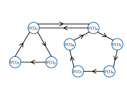
Figure 4: A quiver diagram of three nodes connected with five nodes by a pair of two arrows of vector-like matters.

We shall consider quiver gauge theories with $U(1)^{2k-1}\times U(1)^{2l-1}$ in the presence of vector-like matters. As in Fig. 4, the correspoinding diagram is composed of two diagrams with odd nodes which are connected by a pair of two arrows of vector-like matters. Action is given by two kinds of Eq. (20) showing $U(1)^{2k-1}\times U(1)^{2l-1}$ symmetry and vector-like part of

$$S=\int d^{4}x\biggl{[} \overline{\psi}_{1,2k}i\gamma^{\mu}\bigl{(}\partial_{\mu}+iA^{(1)}_{\mu}-iA^{(2k)}_{\mu}\bigr{)}\psi_{1,2k}+\overline{\psi}_{2k,1}i\gamma^{\mu}\bigl{(}\partial_{\mu}-iA^{(1)}_{\mu}+iA^{(2k)}_{\mu}\bigr{)}\psi_{2k,1}$$

$$-m\overline{\psi_{2k,1}^{C}}\psi_{1,2k}+{\rm h.c.}\biggr{]},$$ (63)

where we assume that the bi-fundamental vector-like matters are charged under the gauge groups of $U(1)_{1}\times U(1)_{2k}$ and that the mass $m$ remains non-zero in the weak gauge coupling limit. In this case, the discrete symmetry is explicitly broken since $\psi_{1,2k}$ is transformed to $\psi_{2,2k+1}$ that is originally absent. For instance, we focus on $U(1)^{3}\times U(1)^{5}$ theory with vector-like matter, which is the case of $k=2$ and $l=3$. Since vector-like matter does not contribute to the chiral anomalies, we have two anomaly-free $U(1)$’s as mentioned above: one denotes $U(1)_{X}$ from $U(1)^{3}$ and another denotes $U(1)_{X^{\prime}}$ from $U(1)^{5}$. Here,

$$U(1)_{X}=\sum_{i=1}^{3}U(1)_{i},\qquad U(1)_{X^{\prime}}=\sum_{i=4}^{8}U(1)_{i},$$ (64)

hence charges of vector-like matters are $(+1,-1)$ and $(-1,+1)$ for $(U(1)_{X},U(1)_{X^{\prime}})$ and other chiral matters are neutral for them. The respective gauge couplings are given by

$$\frac{1}{e_{X}^{2}}=\sum_{i=1}^{3}\frac{1}{g_{i}^{2}},\qquad\frac{1}{e_{X^{\prime}}^{2}}=\sum_{i=4}^{8}\frac{1}{g_{i}^{2}}.$$ (65)

These can be weaker than the original gauge couplings of $g_{i}$’s. Then the WGC for the vector-like matter reads

$$e_{X}^{2}+e_{X^{\prime}}^{2}\geq\frac{m^{2}}{2M_{\mathrm{Pl}}^{2}}.$$ (66)

In the large limit of $k$ and $l$ with a given $m$ and $g_{i}$’s, we find

$$e_{X}^{2}+e_{X^{\prime}}^{2}\sim\frac{g_{i}^{2}}{k}+\frac{g_{i}^{2}}{l}\to 0,$$ (67)

and then the WGC can be violated since the couplings becomes very weak as long as the mass $m$ remains non-zero in the limit of $e_{X}\to 0$ and $e_{X^{\prime}}\to 0$. Note that we now fix $g_{i}$’s but change only $k$ and $l$. This indicates that there exists an upper bounds on the numbers of $U(1)$ gauge groups, $k$ and $l$ as $k+l\lesssim(g_{i}\frac{M_{\mathrm{Pl}}}{m})^{2}$ if the WGC is correct.

3.2 $U(1)^{2k}$

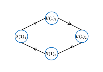
Figure 5: The $\mathbb{Z}_{4}$ symmetric quiver diagram with four nodes.

We consider quiver gauge theories with $U(1)^{2k}$ symmetry as shown in Fig. 1. These types of models are also studied in D-brane models similarly to $U(1)^{2k-1}$ cases. As the simplest model with chiral anomalies, we focus on $U(1)^{4}$ symmetry and this model has four left-handed fermions as in Fig. 5. Divergences of each chiral current are given by

$$\partial\cdot\left(\begin{array}[]{c}j^{1}\\ j^{2}\\ j^{3}\\ j^{4}\end{array}\right)=\left(\begin{array}[]{cccc}0&1&0&-1\\ -1&0&1&0\\ 0&-1&0&1\\ 1&0&-1&0\end{array}\right)\left(\begin{array}[]{c}Q_{1}\\ Q_{2}\\ Q_{3}\\ Q_{4}\end{array}\right),$$ (80)

Since the anomaly coefficient matrix have two zero eigenstate, this model has two independent anomaly-free $U(1)$’s, which are represented by the eigenvectors $(1,0,1,0)^{\mathrm{T}}$ and $(0,1,0,1)^{\mathrm{T}}$. The former relates first node to third one, whereas the latter does second node to fourth one. The independent anomaly-free $U(1)$’s are generally given by

$$U(1)_{X}= cU(1)_{1}+U(1)_{2}+cU(1)_{3}+U(1)_{4},$$ (81)

$$U(1)_{X^{\prime}}= -\frac{1}{c}U(1)_{1}+U(1)_{2}-\frac{1}{c}U(1)_{3}+U(1)_{4},$$ (82)

where $c$ is a free parameter that depends on the D-brane configuration in concrete UV string models [19, 20, 21], and will be a rational number. Otherwise, there exists a global symmetry [52, 53, 54]. The result does not change even if we add bi-fundamental vector-like matters that are charged under only $U(1)_{1}\times U(1)_{3}$ or only $U(1)_{2}\times U(1)_{4}$. For $c=0$, we find $U(1)_{X}=U(1)_{2}+U(1)_{4}$ and $U(1)_{X^{\prime}}=U(1)_{1}+U(1)_{3}$. It is noted that for a general $c$ a linear combination can violate the ${\mathbb{Z}}_{4}$ to ${\mathbb{Z}}_{2}^{2}$ exchanging $1\leftrightarrow 3$ and $2\leftrightarrow 4$. The gauge couplings relevant to the anomaly-free $U(1)$’s read

$$\frac{1}{e_{X}^{2}}= \frac{c^{2}}{g_{1}^{2}}+\frac{1}{g_{2}^{2}}+\frac{c^{2}}{g_{3}^{2}}+\frac{1}{g_{4}^{2}},$$ (83)

$$\frac{1}{e_{X^{\prime}}^{2}}= \frac{1/c^{2}}{g_{1}^{2}}+\frac{1}{g_{2}^{2}}+\frac{1/c^{2}}{g_{3}^{2}}+\frac{1}{g_{4}^{2}}.$$ (84)

In this model, the chiral fermions have non-trivial charges under these anomaly-free $U(1)$’s as shown in Table 1. In the next section, we will numerically study the SWGC in this model by adding a complex scalar.

Extending this model to general theories with $U(1)^{2k}$ is simple, and we can verify that there exists at least two anomaly-free $U(1)$’s in a concrete model. So it is expected that in the large $k$ limit with a given $c$ and a fixed $g_{i}$, anomaly-free gauge couplings become very small as in cases of $U(1)^{2k-1}\times U(1)^{2l-1}$. Then there exists an upper bound on the number of abelian gauge groups if the WGC is correct and a fermion mass remains non-zero in the large $k$ limit.

4 A $U(1)^{4}$ model and the SWGC

In this section, we discuss the detail of $U(1)^{4}$ quiver gauge theory shown in the previous section and its application to the SWGC at the tree level in the presence of a complex scalar field. The motivation for this is to study SWGC in a more realistic (or string-inspired) model with a scalar field. The SWGC shows numerically constraints of a smallness of gauge couplings against Yukawa couplings. We also study a UV completion of 5D orbifold model for it.

4.1 Constraints of the SWGC

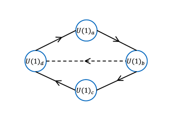
Figure 6: A quiver diagram of $U(1)^{4}$ model including a complex scalar.

Fig. 6 shows a quiver diagram of $U(1)^{4}$ model in the presence of a complex scalar $\varphi$, whose charge is $(+1,-1)$ for $(U(1)_{b},U(1)_{d})$. Due to this scalar field, we have Yukawa couplings of

$$\mathcal{L}_{\rm Yukawa}=-y\varphi\overline{\psi_{ab}^{C}}\psi_{da}-y^{\prime}\varphi^{\dagger}\overline{\psi_{bc}^{C}}\psi_{cd}+\mathrm{h.c.}$$ (85)

This model is inspired by intersecting brane models [30, 32]. No $\mathbb{Z}_{4}$ symmetry exists. This is because $\varphi$ can be written as $\varphi_{bd}$ in the view point of the $U(1)$ charges and hence $\varphi_{bd}$ is transformed to $\varphi_{ca}$ that is originally absent. There could exist $\mathbb{Z}_{2}$ that simultaneously exchanges the labels as $a\leftrightarrow c$ and $b\leftrightarrow d$ for $y=y^{\prime}$, if we can identify $\varphi_{bd}=\varphi_{db}^{\dagger}$. As seen in the previous section, two anomaly-free $U(1)$’s are given by

$$U(1)_{X}= cU(1)_{a}+U(1)_{b}+cU(1)_{c}+U(1)_{d},$$ (86)

$$U(1)_{X^{\prime}}= -\frac{1}{c}U(1)_{a}+U(1)_{b}-\frac{1}{c}U(1)_{c}+U(1)_{d},$$ (87)

where a free parameter $c$ is a rational number and can be fixed in concrete models by the brane configuration in the string theory. The charges of the fields are summarized in Table 1.

Fields	$q_{X}$	$q_{X^{\prime}}$
$\psi_{ab}$	$-1+c$	$-1-1/c$
$\psi_{da}$	$1-c$	$1+1/c$
$\psi_{bc}$	$1-c$	$1+1/c$
$\psi_{cd}$	$-1+c$	$-1-1/c$
$\varphi$	$0$	$0$

Table 1: The charges of fields for the anomaly-free $U(1)_{X}\times U(1)_{X^{\prime}}$ group.

The effective Lagrangian showing two anomaly-free $U(1)$’s may read

$$\mathcal{L}= \sum_{I=ab,bc,cd,da}i\overline{\psi_{I}}{\ooalign{\hfil/\hfil\crcr$D$}}\psi_{I}-|\partial_{\mu}\varphi|^{2}-\frac{1}{4e_{X}^{2}}\bigl{(}F^{(X)}_{\mu\nu}\bigr{)}^{2}-\frac{1}{4e_{X^{\prime}}^{2}}\bigl{(}F_{\mu\nu}^{(X^{\prime})}\bigr{)}^{2}$$ (90)

$$-\bigl{[}y\varphi\overline{\psi_{ab}^{C}}\psi_{da}+y^{\prime}\varphi^{\dagger}\overline{\psi_{bc}^{C}}\psi_{cd}+\mathrm{h.c.}]+\cdots,$$ (91)

where $D_{\mu}=\partial_{\mu}+iq_{X}A_{\mu}^{(X)}+iq_{X^{\prime}}A_{\mu}^{(X^{\prime})}$, gauge bosons relevant to two anomalous $U(1)$’s are neglected since they become massive if the Green-Schwarz mechanism works. Yukawa couplings between the complex scalar and chiral fermions are denoted by $y$ and $y^{\prime}$, which are not the same in general. It is noted that vector-like pairs of $\psi_{ab}+\psi_{da}$ and $\psi_{bc}+\psi_{cd}$ will constitute the Dirac spinors. Now scalar $\varphi$ is neutral under anomaly-free $U(1)$’s and will not be considered for the SWGC. The scalar potential will be neglected hereafter with an assumption that $\varphi$ is sufficiently light at energy scales of our interest since the scalar potential will be model-dependent. To check strong SWGC [11] for $\varphi$ is an interesting issue, but this is left for future work and we focus on the SWGC for fermions with non-trivial anomaly-free gauge charges. Here the anomaly-free gauge couplings are given by

$$\frac{1}{e_{X}^{2}}= \frac{c^{2}}{g_{a}^{2}}+\frac{1}{g_{b}^{2}}+\frac{c^{2}}{g_{c}^{2}}+\frac{1}{g_{d}^{2}},$$ (92)

$$\frac{1}{e_{X^{\prime}}^{2}}= \frac{1/c^{2}}{g_{a}^{2}}+\frac{1}{g_{b}^{2}}+\frac{1/c^{2}}{g_{c}^{2}}+\frac{1}{g_{d}^{2}}.$$ (93)

In the presence of a very light $\varphi$, the SWGC can be expressed as

$$(-1+c)^{2}e_{X}^{2}+\biggl{(}1+\frac{1}{c}\biggr{)}^{2}e_{X^{\prime}}^{2}\geq\frac{M^{2}}{2M_{\mathrm{Pl}}^{2}}+\frac{Y^{2}}{2},$$ (94)

for a test fermion. Here, $Y=y$ and $M=y{\rm Re}(\varphi)$ for a Dirac fermion of $\psi_{ab}+\psi_{da}$, whereas $Y=y^{\prime}$ and $M=y^{\prime}{\rm Re}(\varphi)$ for $\psi_{bc}+\psi_{cd}$. A factor $Y^{2}/2$ is obtained because of the canonical normalization of Re$(\varphi$), and Im$(\varphi$) contributes to the spin-dependent interaction that is not $1/r^{2}$-force. If the scalar is sufficiently heavy, $Y$ does not contribute to the SWGC conditon owing to exponentially damping force and hence the WGC can be easily satisfied. To reduce the number of parameters, we will set $g_{b}=g_{d}=:g$ for simplicity. In the next subsection, we will study this situation realized in the 5D orbifold model. Thus this equation can be rewritten as

$$\frac{(1-c)^{2}}{c^{2}(g^{2}/g_{a}^{2}+g^{2}/g_{c}^{2})+2}+\frac{(1+1/c)^{2}}{(1/c^{2})(g^{2}/g_{a}^{2}+g^{2}/g_{c}^{2})+2}\gtrsim\frac{1}{2}\bigg{(}\frac{Y}{g}\bigg{)}^{2}.$$ (95)

Here, the masses are neglected because $M/M_{\rm Pl}\ll 1$ is numerically expected in the effective field theory. Indeed, there is almost no change in appearance of the plots for $M/gM_{\rm Pl}\lesssim 0.1$, where $gM_{\rm Pl}$ is expected as a cutoff scale [3], when the scalar is massless. It is noted also that a gauge boson in either $U(1)_{X}$ or $U(1)_{X^{\prime}}$ may be massive owing to the Stückelberg coupling and then either $e_{X}$ or $e_{X^{\prime}}$ vanishes in Eq. (95).

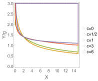
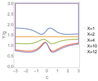
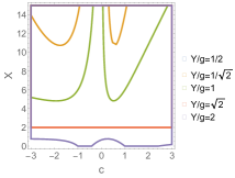
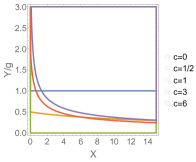
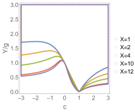
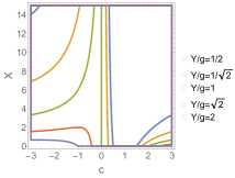
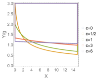
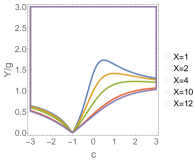
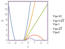
Figure 7: Plots of the SWGC constraints in $(X,Y/g)$-, $(c,Y/g)$- and $(c,X)$-planes. The top panels plot the constraints of Eq. (95). The middle (bottom) figures show the similar plots with $e_{X^{\prime}}=0$ ($e_{X}=0$), when $U(1)_{X}$ ($U(1)_{X^{\prime}}$) gauge group survives in low energy limit. The condition is saturated on each lines, below which there exist an allowed region. In the presence of mass, the SWGC is violated on each line.

In the top panels of Fig. 7, we show the plots of the SWGC (95) in the $(X,Y/g)$-, $(c,Y/g)$- and $(c,X)$-planes, where $X:=g^{2}/g_{a}^{2}+g^{2}/g_{c}^{2}$. The each line saturates Eq. (95), hence the allowed region exists below them. In the presence of the mass, the SWGC is violated on each line. Note that these plots are symmetric under $c\to-1/c$ owing to the definition of the anomaly-free $U(1)$’s. A region for a large Yukawa coupling is excluded by the SWGC. For a large $X$, the constraint becomes tighter. In other words, a big discrepancy between gauge couplings is disfavored. It turns out that the constraint becomes stronger near $c=\pm 1$ because either $e_{X}$ or $e_{X^{\prime}}$ vanishes then. We find also that the constraint is independent of $c$ for special values of $X=2$ and $Y/g=\sqrt{2}$. This is because for $X=2$ the left hand side of Eq. (95) becomes unity and hence for $Y/g\geq\sqrt{2}$ the SWGC is then violated in the presence of the mass term. We can find also that the constraint becomes weaker as the $c>0$ increases in the top-left panel for $X>2$, because either $e_{X}$ or $e_{X^{\prime}}$ gets stronger then whereas the constraint does not depend on $c$ for $X\ll 1$. It is noted that in the string theory $c$ depends on the D-brane configuration and the couplings depend on moduli fields with the fixed configuration. The middle (bottom) figures show the similar plots with $e_{X^{\prime}}=0$ ($e_{X}=0$), when only a gauge boson of $U(1)_{X}$ ($U(1)_{X^{\prime}}$) remains massless and mediates the long-range repulsive force. In these cases, the condition of the SWGC tends to give tighter constraints.

4.2 A $U(1)^{4}$ model from $S^{1}/\mathbb{Z}_{2}$ orbifold and the SWGC

Fields	$U(2)$	$U(1)_{a}$	$U(1)_{c}$
$A_{M}$	adj	$0$	$0$
$\Psi_{a}$	$\bm{2}_{1/2}$	$-1$	$0$
$\Psi_{c}$	$\overline{\bm{2}}_{-1/2}$	$0$	$+1$
$A^{(a)}_{M}$	$0$	adj	$0$
$A^{(c)}_{M}$	$0$	$0$	adj

Table 2: Table of the field contents and their charges in 5D model for realizing $U(1)^{4}$ gauge theory in 4D. Subscripts of $U(2)$ representation for fermions are $U(1)$ charges against the overall $U(1)\in U(2)$.

We consider a 5D gauge theory with $U(2)\times U(1)_{a}\times U(1)_{c}$ on the $S^{1}/\mathbb{Z}_{2}$ orbifold for realizing chiral fermions. The purpose of this subsection is to give a concrete Yukawa coupling associated with the gauge coupling and a relation between gauge couplings as in the previous subsection via the symmetry breaking of $U(2)\to U(1)_{b}\times U(1)_{d}$ by an orbifold projection. The fields contents and their representations are exhibited in Table 2. The 5D action is given by

$$S_{\text{5D}}=\int_{M_{4}\times S^{1}/\mathbb{Z}_{2}}d^{4}xdy\,\sqrt{-G_{5}}\biggl{[} \frac{1}{2\kappa_{5}^{2}}\mathcal{R}_{5}-\frac{1}{2\hat{g}_{2}^{2}}\mathrm{tr}(F_{MN})^{2}-\frac{1}{4\hat{g}_{a}^{2}}\bigl{(}F^{(a)}_{MN}\bigr{)}^{2}-\frac{1}{4\hat{g}_{c}^{2}}\bigl{(}F^{(c)}_{MN}\bigr{)}^{2}$$

$$+\overline{\Psi_{a}}(i{\ooalign{\hfil/\hfil\crcr$D$}}-M_{a})\Psi_{a}+\overline{\Psi_{c}}(i{\ooalign{\hfil/\hfil\crcr$D$}}-M_{c})\Psi_{c}\biggr{]},$$ (100)

where $M=0,1,2,3,y$, $D_{M}=\nabla_{M}+iA_{M}+i\hat{q}_{a}A^{(a)}_{M}+i\hat{q}_{c}A^{(c)}_{M}$ and $\hat{q}_{a}$ and $\hat{q}_{c}$ are the charges of $U(1)_{a}$ and $U(1)_{c}$ respectively. 5D Chern Simons terms associated with 4D Green-Schwarz mechanism is neglected as already noted. The field strengths are given by $F_{MN}=\partial_{M}A_{N}-\partial_{N}A_{M}+i[A_{M},A_{N}]$ and $F^{(a,c)}_{MN}=\partial_{M}A^{(a,c)}_{N}-\partial_{N}A^{(a,c)}_{M}$ for the non-abelian gauge field and abelian gauge fields respectively. The normalization of generator of $U(2)$ is chosen as $\mathrm{tr}(T_{a}T_{b})=\delta_{ab}/2$, hence the $U(2)$ gauge field is expanded as $A_{M}=\frac{{\mbox{1}\mbox{l}}_{2}}{2}A_{M}^{(0)}+\frac{\sigma^{a}}{2}A_{M}^{(a)}$, where ${\mbox{1}\mbox{l}}_{2}$ is $2\times 2$ identity matrix and $\sigma^{a}$’s $(a=1,2,3)$ are the Pauli matrices. Since the covariant derivative is acting on $\Psi_{a}$ as $D_{M}\Psi_{a}\ni iA_{M}\Psi_{a}=i\frac{{\mbox{1}\mbox{l}}_{2}}{2}A_{M}^{(0)}\Psi_{a}+\cdots$, $\Psi_{a}$ has $1/2$ charge against the overall $U(1)$. This is similar to $\Psi_{c}$, which has the opposite $U(1)$ charge. Here, $\Psi_{a,c}=(\psi_{a,c1},\psi_{a,c2})^{\mathrm{T}}$ are doublets for the $SU(2)$ and $\psi_{a,c}$ are the 4D Dirac spinors. The metric of $M_{4}\times S^{1}/\mathbb{Z}_{2}$ is written by $ds_{5}^{2}=e^{-\sigma}g_{\mu\nu}dx^{\mu}dx^{\nu}+e^{2\sigma}dy^{2}$, where $\sigma$ is the radion field, and gives 4D Einstein frame. The size of $S^{1}/\mathbb{Z}_{2}$ is assumed to be $\pi L$ and we take $\langle\sigma\rangle=0$ without loss of generality. The graviphoton $g_{\mu y}$ is dropped since it is parity odd while the 4D graviton $g_{\mu\nu}$ remains massless. Then, the massive graviphoton mediates the short-range force among particles which have the Kaluza-Klein (KK) charges, and does not contribute to the SWGC condition. On top of the usual periodic boundary condition of $S^{1}$, the orbifold boundary conditon is given by

$$PA_{M}(x,-y)P^{-1} =\eta_{A}A_{M}(x,y),\quad A_{M}^{(a,c)}(x,-y)=\eta_{A}A_{M}^{(a,c)}(x,y),$$ (101)

$$P\Psi_{a,d}(x,-y) =\gamma_{5}\Psi_{a,d}(x,y),$$ (102)

where $P=\mathrm{diag}(+1,-1)\in U(2)$, $\eta_{A}=1$ for $M=\mu=0,1,2,3$ and $\eta_{A}=-1$ for $M=y$. Thus 4D massless modes read

$$A_{\mu}=\left(\begin{array}[]{cc}A^{(b)}_{\mu}&\\ &A^{(d)}_{\mu}\end{array}\right),\quad A_{y}=\left(\begin{array}[]{cc}&i\varphi/\sqrt{2}\\ -i\varphi^{\dagger}/\sqrt{2}&\end{array}\right),\quad A^{(a)}_{\mu},\quad A^{(c)}_{\mu},$$ (107)

$$\psi_{a1R},~{}\psi_{a2L},\quad\psi_{c1R},~{}\psi_{c2L}.$$ (108)

where $A^{(b)}_{\mu}:=\frac{1}{2}(A_{\mu}^{(0)}+A_{\mu}^{(3)})$, $A^{(d)}_{\mu}:=\frac{1}{2}(A_{\mu}^{(0)}-A_{\mu}^{(3)})$, $\varphi=-(iA^{(1)}_{y}+A^{(2)}_{y})/\sqrt{2}$ is the complex scalar originating from the $W$-boson of $y$-direction, and the $\psi_{L}$ ($\psi_{R}$) is the left-handed (right-handed) chiral fermion in 4D. It turns out that there exists the gauge symmetry of $U(1)_{a}\times U(1)_{b}\times U(1)_{c}\times U(1)_{d}$. As seen from the zero mode basis in the $U(2)$ gauge bosons, we find matter charges for the gauge symmetry: As for $(U(1)_{a},U(1)_{b},U(1)_{c},U(1)_{d})$, $\psi_{a1R}^{C}\equiv\psi_{ab}:(+1,-1,0,0)$, $\psi_{c1R}^{C}\equiv\psi_{bc}:(0,+1,-1,0)$, $\psi_{c2L}\equiv\psi_{cd}:(0,0,1,-1)$, $\psi_{a2L}\equiv\psi_{da}:(-1,0,0,1)$ and $\varphi:(0,1,0,-1)$. This is the same field content as in the previous subsection, hence $\varphi$ is a neutral scalar under anomaly-free $U(1)$’s and will not be considered for the SWGC. The scalar potential will be neglected as previously noted since the scalar potential including radion will depend on the model and the radion stabilization. Deriving the scalar potential and checking the strong SWGC for this is left for future work.

The 4D parameters are given by the 5D parameters with an assumption of $\langle\sigma\rangle=0$. For the details, see Appendix C. The 4D Planck mass is associated with the 5D gravitational coupling $\kappa_{5}$ as

$$M_{\mathrm{Pl}}^{2}=\frac{\pi L}{\kappa_{5}^{2}},$$ (109)

and the gauge couplings in 4D are expressed by

$$\frac{2}{g^{2}_{2}}:=\frac{1}{g_{b}^{2}}=\frac{1}{g_{d}^{2}}=\frac{2\pi L}{\hat{g}_{2}^{2}},\qquad\frac{1}{g_{a}^{2}}:=\frac{\pi L}{\hat{g}_{a}^{2}},\quad\frac{1}{g_{c}^{2}}:=\frac{\pi L}{\hat{g}_{c}^{2}}.$$ (110)

This is because we have the gauge kinetic term ${\mathcal{L}}=-2/4g_{2}^{2}\bigl{(}F_{\mu\nu}^{(b)}\bigr{)}^{2}-2/4g_{2}^{2}\bigl{(}F_{\mu\nu}^{(d)}\bigr{)}^{2}$ via the symmetry breaking of $U(2)\to U(1)_{b}\times U(1)_{d}$. With these, the anomaly-free couplings are defined as previously:

$$\frac{1}{e_{X}^{2}}= \frac{c^{2}}{g_{a}^{2}}+\frac{2}{g_{2}^{2}}+\frac{c^{2}}{g_{c}^{2}}+\frac{2}{g_{2}^{2}},$$ (111)

$$\frac{1}{e_{X^{\prime}}^{2}}= \frac{1/c^{2}}{g_{a}^{2}}+\frac{2}{g_{2}^{2}}+\frac{1/c^{2}}{g_{c}^{2}}+\frac{2}{g_{2}^{2}},$$ (112)

where a free parameter $c$ is a rational number.

The Yukawa couplings between $\varphi$ and $\psi$’s are given by

$$y=y^{\prime}=\frac{\hat{g}_{2}}{\sqrt{2\pi L}}=\frac{g_{2}}{\sqrt{2}}.$$ (113)

Here, $y$ and $y^{\prime}$ are the same definition as in the previous subsection. This equation relates the Yukawa coupling to the gauge coupling. In the presence of a light $\mathrm{Re}(\varphi)$ and the radion, the SWGC inequality for zero mode fermions reads

$$(1-c)^{2}e_{X}^{2}+\biggl{(}1+\frac{1}{c}\biggr{)}^{2}e_{X^{\prime}}^{2}\geq\frac{y^{2}}{2}+\left(\frac{1}{2}+\frac{1}{6}\right)\frac{M^{2}}{M_{\mathrm{Pl}}^{2}}$$ (114)

where $M$ has the same definition as in the previous subsection and $1/6$ comes from the radion exchange via $ye^{-\sigma_{c}/\sqrt{6}M_{\rm Pl}}{\rm Re}(\varphi)\overline{\psi}\psi$ with the canonically normalized radion $\sigma_{c}=\sqrt{3/2}M_{\rm Pl}\sigma$. We have neglected momentum-dependent terms induced by the radion exchange with terms of $\overline{\psi}\gamma^{\mu}\psi\partial_{\mu}\sigma$. If $\mathrm{Re}(\varphi)$ is sufficiently heavy, the yukawa interaction in this equation can be neglected and the WGC can be then easily satisfied. Gravitational interactions including radion exchange will be numerically neglected below as in the previous subsection owing to the Planck-suppressed interaction within the effective field theory. For $M/g_{2}M_{\rm Pl}\lesssim 0.1$ and $p/g_{2}M_{\rm Pl}\lesssim 0.1$, where $p$ is the momentum of a test fermion, there are not significant differences compared to the plots shown below. Substituting the above couplings given by Eqs. (111)–(113) to Eq. (114), we then find the SWGC condition

$$\frac{(1-c)^{2}}{(c^{2}/2)(g_{2}^{2}/g_{a}^{2}+g_{2}^{2}/g_{c}^{2})+2}+\frac{(1+1/c)^{2}}{(1/2c^{2})(g_{2}^{2}/g_{a}^{2}+g_{2}^{2}/g_{c}^{2})+2}\gtrsim\frac{1}{4}.$$ (115)

This is also obtained when the parameters in Eq. (95) are replaced as $g^{2}\to g^{2}_{2}/2$ and $(Y/g)^{2}\to 1/2$. This gives a constraint between $c$ and $X:=g_{2}^{2}/g_{a}^{2}+g_{2}^{2}/g_{c}^{2}$.

As for the KK modes or the massive parity odd ones, a similar equation to Eq. (114) will be hold. It is noted that massive gauge bosons do not contribute to long-range forces and all bosons including scalar zero mode are neutral under anomaly-free $U(1)$’s and fermions with non-trivial gauge charges are considered for the SWGC. Parity odd fermions of $\psi_{a1L},~{}\psi_{a2R},\psi_{c1L}$ and $\psi_{a2R}$ have opposite charges to zero mode fermions. KK modes of a field have the same charge as that of the lightest mode. Yukawa couplings that are invariant under ${\mathbb{Z}}_{2}$ projection are given by $\phi_{\rm even}\psi_{\rm even}\psi_{\rm even}$, $\phi_{\rm even}\psi_{\rm odd}\psi_{\rm odd}$,  $\phi_{\rm odd}\psi_{\rm odd}\psi_{\rm even}$, where $\phi_{\rm even}$ ($\phi_{\rm odd}$) is an even (odd) parity scalar and $\psi_{\rm even}$ ($\psi_{\rm odd}$) is an even (odd) parity fermion. As massive scalars do not contribute to a long-range force, Yukawa couplings relevant to the SWGC are associated with $\varphi$: $\varphi\psi_{\rm even}\psi_{\rm even},~{}\varphi\psi_{\rm odd}\psi_{\rm odd}$. After integration over the extra dimension, we will find Yukawa couplings of $y\varphi\psi_{n}^{\prime}\psi_{n}$ in addition to KK mass terms $(n/L)\overline{\psi}_{n}\psi_{n}+(n/L)\overline{\psi^{\prime}}_{n}\psi_{n}^{\prime}$ for $n$-th KK modes with the canonically normalized kinetic terms (up to the radion dependence). Then $n$-th KK mass eigenstates will have mass $M^{2}=(n/L\pm y{\rm Re}(\varphi))^{2}$. As the SWGC could be violated by heavy KK modes, it is necessary to check whether lighter modes including the zero modes satisfy the SWGC.

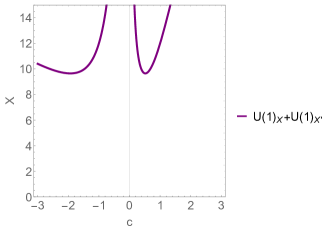
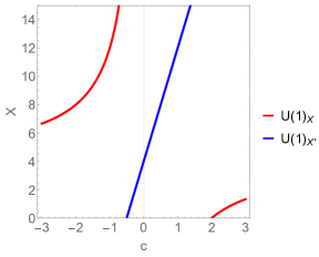
Figure 8: The left panel: Plots of the SWGC conditons (115) in the $(c,X)$-planes. The condition is saturated on each lines, below which there exist an allowed region. In the presence of mass, the SWGC is violated on each line. The right panel: A similar plot with only $U(1)_{X}$ (red) and one with only $U(1)_{X^{\prime}}$ (blue).

Fig. 8 shows the plots of the SWGC (115) in the $(c,X)$ plane. The each line saturates Eq. (115), hence the allowed region exists below them. In the presence of mass, the SWGC is violated on each line. The these plots are symmetric under $c\to-1/c$. The left panel shows the constraint when there exists two anomaly-free $U(1)$’s. This is very similar to the top-right one of Fig. 7 for a small value of Yukawa. For a large $X$, not only $U(1)_{b}\times U(1)_{d}$ gauge coupling but also Yukawa coupling $\propto g_{2}$ become much stronger than $g_{a}$ or $g_{c}$, and hence there exist an upper bound on $X$. It is noted that in the context of the string theory a large $X$ may imply a big discrepancy among moduli vacuum expectation values. In the vincity of $c=\pm 1$, matter becomes neutral against either one of the anomaly-free $U(1)$’s, then the constraint becomes tighter. In the right panel, plots show the SWGC constraint with $e_{X}=0$ or $e_{X^{\prime}}=0$, when only the gauge boson of either $U(1)_{X}$ or $U(1)_{X^{\prime}}$ remains massless owing to a Stückelberg coupling as often seen in concrete string models.

5 Conclusion

We have studied the (S)WGC in several types of quiver gauge theories with $U(1)^{k}$ gauge symmetry in the presence of bi-fundamental chiral fermions leading to the chiral anomalies, which is supposed to be canceled by the Green-Schwarz mechanism. The theories which we consider possesses a cyclic ${\mathbb{Z}}_{k}$ symmetry associated with a shift of the label of the gauge groups. As a consequence of this, we can study anomalies in the models systematically and the (S)WGC constraints on the gauge couplings. We identified concretely the anomaly-free $U(1)$’s and their gauge couplings obtained via linear combinations of the original $U(1)$’s. Then, ${\mathbb{Z}}_{k}$ symmetry can be broken in general. In the large $k$ limit, an anomaly-free gauge coupling becomes very weak as $e\sim k^{-1/2}$, and there exists an upper bound on $k$ if the WGC is correct and the mass for a test particle remains in the large $k$ limit. This may be regarded as an example of the weak coupling conjecture. For quiver theories with $U(1)^{2k-1}$, an unique anomaly-free $U(1)$ is proportional to $\sum_{i=1}^{2k-1}U(1)_{i}$ and all matters are neutral under the anomaly-free $U(1)$. There exist charged matters in the presence of vector-like pairs, and $\mathbb{Z}_{2k-1}$ symmetry is broken then. For quiver theories with $U(1)^{2k}$ gauge symmetry, there exist two anomaly-free $U(1)$’s and charged matters under these gauge groups, and $\mathbb{Z}_{2k}$ symmetry is broken in general. Even if the gauge couplings of the the anomaly-free $U(1)$’s receive quantum corrections, the IR couplings will remain very weak in the large $k$ limit since $U(1)$ couplings are generally asymptotic non-free as far as the pertubation theory is valid.

We have numerically studied also the SWGC in $U(1)^{4}$ theory in the presence of a complex scalar field, and construct a similar model based on a 5D orbifold. It turns out that a much larger Yukawa coupling than gauge couplings is forbidden and also that a big discrepancy among gauge couplings is disfavored. A special linear combination for realizing the anomaly-free $U(1)$’s can be also be disfavored, since matter charge becomes small then.

So far, we neglected kinetic mixings $\chi_{ij}F_{\mu\nu}^{i}F^{j\mu\nu}$ among gauge fields. If we have such terms, we may have a kinetic mixing of $\chi F_{\mu\nu}^{X}F^{X^{\prime}\mu\nu}$, where $\chi\sim\sum_{i,j}^{k}\chi_{ij}c_{i}c_{j}^{\prime}$, for anomaly-free $U(1)_{X}=\sum_{i}c_{i}U(1)_{i}$ and $U(1)_{X^{\prime}}=\sum_{i}c_{i}^{\prime}U(1)_{i}$ with $c_{i}$’s $={\mathcal{O}}(1)$. If the mixing $\chi$ is at most of ${\mathcal{O}}(k^{3/2-\alpha})~{}(\alpha>0)$ in the large $k$ limit, the WGC can still be violated as in Sec. 3. This is because the canonically normalized mixing is given by $e_{X}e_{X^{\prime}}\chi$ and hence an induced coupling of a fermion to an anomay-free gauge field is proportional to $e_{X}^{2}e_{X^{\prime}}\chi$ or $e_{X}e_{X^{\prime}}^{2}\chi$ that are scaling as $k^{-\alpha}$ then. However, if $\chi={\mathcal{O}}(k^{2})$ in the large $k$ limit, the WGC can be satisfied.

In the Sec. 4, the scalar $\varphi$ is a singlet under the anomaly-free gauge groups, and we did not discuss the detail of the scalar potential in addition to the radion. Hence it may be an interesting challenge to check the strong SWGC within a fixed model. This is left for future work.

It will be worth to investigate the (S)WGC in theories with more general gauge groups. In actual string compactifications, the number of closed string axions is known to be finite and depends on the Hodge number of compactification manifold. Some of the axions play an important role to cancel anomalies through the Green-Schwarz mechanism. Hence, the number of anomalous $U(1)$ gauge theories, which is $k-1$ or $k-2$ in our cases, should be constrained by the number of such axions. If the anomalies are independent among the anomalous theories, the number of anomalous $U(1)$’s can be less than that of axions for anomaly cancellation. Also in the string theory, the conjecture would constrain brane configuration and moduli values. If one starts with 10D super Yang-Mills theory, 4D effective action including an anomaly-free $U(1)$ may be given by [55, 56]

$$\mathcal{L}=-c\frac{S}{4}(F_{\mu\nu})^{2}-\frac{\vartheta(\tau)}{\sqrt{S}}\phi\overline{\psi}\psi+\cdots,$$ (116)

where $S$ is the 4D dilaton, $\tau$ is a complex structure modulus, and a rational number $c$ originates from a linear combination of $U(1)$’s depends on brane configuration of the number of branes and magnetic fluxes. The SWGC of $e^{2}\gtrsim y^{2}$ (up to mass term) for matter fermion may read

$$c\lesssim\frac{1}{|\vartheta(\tau)|^{2}}.$$ (117)

However, it will be required a deep understanding of the string theory or concrete effective field theories including (non-abelian) Dirac-Born-Infeld action to study the SWGC constraints on moduli space for consistent gauge theories in the presence of the Green-Schwarz mechanism. This is also left for future works.

Appendix A Anomalies in string-inspired (SUSY) gauge theories

We discuss anomaly-free $U(1)$’s in $U(N)^{k}$ quiver gauge theories inspired by the string theory. We focus only on certain types of quiver theories considered in Sec. 3 in this section. Hereafter, $N_{a}$ denotes the rank of the gauge group of $U(N_{a})$ at the $a$-node, and $n_{ab}$ shows the number of bi-fundamental matter fields which correspond to that of arrows connecting between $a$-node and $b$-node in the quiver diagram.

A.1 $U(N)^{3}$

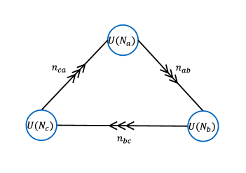
Figure 9: A quiver diagram of $U(N)^{3}$ gauge theory.

We consider a $U(N)^{3}$ quiver gauge theory as shown in Fig. 9, and identify an anomaly-free $U(1)$. To this end, we calculate chiral anomalies and mixed anomalies. Then, we find the constraints on the ranks of gauge groups and the numbers of generations. For a consistent theory, the non-abelian cubic anomalies $\mathcal{A}_{SU(N_{a,b,c})^{3}}$ give the following constraints,

$$\mathcal{A}_{SU(N_{a})^{3}}\propto (n_{ab}N_{b}-n_{ca}N_{c})\equiv 0,$$ (118)

$$\mathcal{A}_{SU(N_{b})^{3}}\propto (n_{bc}N_{c}-n_{ab}N_{a})\equiv 0,$$ (119)

$$\mathcal{A}_{SU(N_{c})^{3}}\propto (n_{ca}N_{a}-n_{bc}N_{b})\equiv 0.$$ (120)

With these equations, the ranks of the gauge groups are related as

$$N_{a}=\frac{n_{bc}}{n_{ab}}N_{c}\in\mathbb{N},\quad N_{b}=\frac{n_{ca}}{n_{ab}}N_{c}\in\mathbb{N}.$$ (121)

Thus, we find $N_{a}=N_{b}=N_{c}$ for $n_{ab}=n_{bc}=n_{ca}$. The divergences of the chiral currents $j^{a,b,c}$ for $U(1)_{a,b,c}$ are given by

$$\partial\cdot j^{a}= N_{a}(N_{b}n_{ab}Q_{b}-N_{c}n_{ac}Q_{c})+N_{a}(n_{ab}N_{b}-n_{ca}N_{c})Q_{a}+\mathcal{A}_{U(1)_{a}G^{2}},$$ (122)

$$\partial\cdot j^{b}= N_{b}(N_{c}n_{bc}Q_{c}-N_{a}n_{ab}Q_{a})+N_{b}(n_{bc}N_{c}-n_{ab}N_{a})Q_{b}+\mathcal{A}_{U(1)_{b}G^{2}},$$ (123)

$$\partial\cdot j^{c}= N_{c}(N_{a}n_{ca}Q_{a}-N_{b}n_{bc}Q_{b})+N_{c}(n_{ca}N_{a}-n_{bc}N_{b})Q_{c}+\mathcal{A}_{U(1)_{c}G^{2}},$$ (124)

where $Q_{x}=Q^{U(1)_{x}}+\frac{1}{N_{x}}Q^{SU(N_{x})}$, $Q^{G_{x}}=\frac{1}{16\pi^{2}}\epsilon^{\mu\nu\rho\sigma}\mathrm{tr}(F^{(x)}_{\mu\nu}F^{(x)}_{\rho\sigma})$ for $x=a,b,c$, and tr$(T^{i}T^{j})=\delta^{ij}/2$ for $U(N)$ generators $T^{i}$’s. These include anomalies of $U(1)^{3}$, $U(1)SU(N)^{2}$ and the mixed anomalies between the gravity and $U(1)$’s, which are denoted by $\mathcal{A}_{U(1)_{a,b,c}G^{2}}$. We impose that they are vanishing:

$$\mathcal{A}_{U(1)_{a}G^{2}}\propto N_{a}(n_{ab}N_{b}-n_{ca}N_{c})\equiv 0,$$ (125)

$$\mathcal{A}_{U(1)_{b}G^{2}}\propto N_{b}(n_{bc}N_{c}-n_{ab}N_{a})\equiv 0,$$ (126)

$$\mathcal{A}_{U(1)_{c}G^{2}}\propto N_{c}(n_{ca}N_{a}-n_{bc}N_{b})\equiv 0.$$ (127)

This is the same condition as in the non-abelian anomalies. There are not exist charged fields under all $(U(1)_{a},U(1)_{b},U(1)_{c})$, then the anomaly between $U(1)_{a}U(1)_{b}U(1)_{c}$ vanishes automatically. Then we find

$$\partial\cdot j^{a}\equiv N_{a}(N_{b}n_{ab}Q_{b}-N_{c}n_{ac}Q_{c}),$$ (128)

$$\partial\cdot j^{b}\equiv N_{b}(N_{c}n_{bc}Q_{c}-N_{a}n_{ab}Q_{a}),$$ (129)

$$\partial\cdot j^{c}\equiv N_{c}(N_{a}n_{ca}Q_{a}-N_{b}n_{bc}Q_{b}).$$ (130)

To identify the anomaly-free $U(1)$ we define it as

$$U(1)_{X}:=\frac{c_{a}}{N_{a}}U(1)_{a}+\frac{c_{b}}{N_{b}}U(1)_{b}+\frac{c_{c}}{N_{c}}U(1)_{c},$$ (131)

and we impose that the divergence of the current associated with $U(1)_{X}$ vanishes

$$\partial\cdot j^{X}= \sum_{x=a,b,c}\frac{c_{x}}{N_{x}}\partial\cdot j^{x}$$

$$= N_{a}(c_{c}n_{ca}-c_{b}n_{ab})Q_{a}+N_{b}(c_{a}n_{ab}-c_{c}n_{bc})Q_{b}+N_{c}(c_{b}n_{bc}-c_{a}n_{ca})Q_{c}\equiv 0.$$ (132)

From this equation, the coefficients satisfy the following conditions

$$c_{a}=\frac{n_{bc}}{n_{ab}}c_{c},\quad c_{b}=\frac{n_{ca}}{n_{ab}}c_{c}.$$ (133)

We take $c_{c}=1$ and use Eqs. (121) and (133), then the anomaly-free $U(1)$ is given by

$$U(1)_{X}=\frac{c_{c}}{N_{c}}\bigl{(}U(1)_{a}+U(1)_{b}+U(1)_{c}\bigr{)}.$$ (134)

It is noted that all fields are neutral matter under this anomaly-free $U(1)$. The anomaly-free gauge coupling is given by

$$\frac{1}{e_{X}^{2}}=\frac{1}{g_{a}^{2}}+\frac{1}{g_{b}^{2}}+\frac{1}{g_{c}^{2}}.$$ (135)

A.2 $U(N)^{4}$

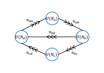
Figure 10: $U(N)^{4}$ quiver diagram.

In this case, we impose that the anomaly coefficients of non-abelian cubic anomaly are vanishing:

$$\mathcal{A}_{SU(N_{a})^{3}}\propto (n_{ab}N_{b}-n_{da}N_{d})\equiv 0,$$ (136)

$$\mathcal{A}_{SU(N_{b})^{3}}\propto (-n_{ab}N_{a}+n_{bc}N_{c}+n_{bd}N_{d})\equiv 0,$$ (137)

$$\mathcal{A}_{SU(N_{c})^{3}}\propto (-n_{bc}N_{b}+n_{cd}N_{d})\equiv 0,$$ (138)

$$\mathcal{A}_{SU(N_{d})^{3}}\propto (n_{da}N_{a}-n_{bd}N_{b}-n_{cd}N_{c})\equiv 0.$$ (139)

Solving these equations, we find that the ranks of gauge groups and the numbers of generations have the following relations,

$$N_{b}=\frac{n_{da}}{n_{ab}}N_{d}\in\mathbb{N},\quad N_{c}=\frac{n_{da}}{n_{cd}}\biggl{[}N_{a}-\biggl{(}\frac{n_{bd}}{n_{ab}}\biggr{)}N_{d}\biggr{]}\in\mathbb{N},\quad\frac{n_{da}}{n_{ab}}=\frac{n_{cd}}{n_{bc}}.$$ (140)

The cancellation of the mixed anomaly between the gravity and $U(1)$’s imposes the same constraints as above:

$$\mathcal{A}_{U(1)_{a}G^{2}}\propto N_{a}(n_{ab}N_{b}-n_{da}N_{d})\equiv 0,$$ (141)

$$\mathcal{A}_{U(1)_{b}G^{2}}\propto N_{b}(-n_{ab}N_{a}+n_{bc}N_{c}+n_{bd}N_{d})\equiv 0,$$ (142)

$$\mathcal{A}_{U(1)_{c}G^{2}}\propto N_{c}(-n_{bc}N_{b}+n_{cd}N_{d})\equiv 0,$$ (143)

$$\mathcal{A}_{U(1)_{d}G^{2}}\propto N_{d}(n_{da}N_{a}-n_{bd}N_{b}-n_{cd}N_{c})\equiv 0.$$ (144)

The divergences of the $U(1)$ currents are expressed as

$$\partial\cdot j^{a}\equiv N_{a}(N_{b}n_{ab}Q_{b}-N_{d}n_{da}Q_{d}),$$ (145)

$$\partial\cdot j^{b}\equiv N_{b}(-N_{a}n_{ab}Q_{a}+N_{b}n_{bc}Q_{c}+N_{d}n_{bd}Q_{d}),$$ (146)

$$\partial\cdot j^{c}\equiv N_{c}(-N_{b}n_{bc}Q_{b}+N_{d}n_{cd}Q_{d}),$$ (147)

$$\partial\cdot j^{d}\equiv N_{d}(N_{a}n_{da}Q_{a}-N_{b}n_{bd}Q_{b}-N_{c}n_{cd}Q_{c}),$$ (148)

where we used vanishing conditions of non-abelian anomalies. We define the anomaly-free $U(1)$ by the following equation as in the previous subsection

$$U(1)_{X}:=\frac{c_{a}}{N_{a}}U(1)_{a}+\frac{c_{b}}{N_{b}}U(1)_{b}+\frac{c_{c}}{N_{c}}U(1)_{c}+\frac{c_{d}}{N_{d}}U(1)_{d},$$ (149)

and impose the current divergence associated with this $U(1)_{X}$ is vanishing

$$\sum_{x=a,b,c,d}\frac{c_{x}}{N_{x}}\partial\cdot j^{x}= N_{a}(-c_{b}n_{ab}+n_{d}n_{da})Q_{a}+N_{b}(c_{a}n_{ab}-c_{c}n_{bc}-c_{d}n_{bd})Q_{b}$$

$$+N_{c}(c_{b}n_{bc}-c_{d}n_{cd})Q_{c}+N_{d}(-c_{a}n_{da}+c_{b}n_{bd}+c_{c}n_{cd})Q_{d}$$

$$\equiv 0.$$ (150)

Solving these equations for the coefficients $c_{x}$, we get the following relations

$$c_{b}=\frac{n_{da}}{n_{ab}}c_{d},\quad c_{c}=\frac{n_{da}}{n_{cd}}\biggl{[}c_{a}-\biggl{(}\frac{n_{bd}}{n_{ab}}\biggr{)}c_{d}\biggr{]},\quad\frac{n_{da}}{n_{ab}}=\frac{n_{cd}}{n_{bc}}.$$ (151)

From Eqs. (140) and (151), the coefficient $c_{a}$ (or $c_{b}$) is a free parameter. In oder to solve these equations, we shall impose some assumptions. Here we will list some examples satisfying these equations.

• $\forall~{}N=1$

  • $n_{bd}=0$
    A solution is

    $$N_{a}=N_{b}=N_{c}=N_{d}=1,\quad n_{ab}=n_{bc}=n_{cd}=n_{da},\quad n_{bd}=0.$$ (152)

    This is similar to the quiver gauge theory shown in Fig. 5. The two independent anomaly-free $U(1)$’s are generally given by Eqs. (81) and (82), and the corresponding gauge couplings are expressed as Eq. (83) and (84).

  • $n_{bd}=2$
    A solutions is given by

    $$N_{a}=N_{b}=N_{c}=N_{d}=1,\quad n_{ab}=n_{da}=-n_{bc}=-n_{cd}=1,\quad n_{bd}=2.$$ (153)

    The minus sign represents the opposite arrow of Fig. 10. The independent anomaly-free $U(1)$’s are defined by

    $$U(1)_{X}= cU(1)_{a}+U(1)_{b}+(2-c)U(1)_{c}+U(1)_{d},$$ (154)

    $$U(1)_{X^{\prime}}= \frac{c-3}{c-1}U(1)_{a}+U(1)_{b}+\frac{c+1}{c-1}U(1)_{c}+U(1)_{d}.$$ (155)

    For these anomaly-free $U(1)$’s, $bd$ matters are neutral. The anomaly-free gauge couplings are given by

    $$\frac{1}{e_{X}^{2}}= \frac{c^{2}}{g_{a}^{2}}+\frac{1}{g_{b}^{2}}+\frac{(2-c)^{2}}{g_{c}^{2}}+\frac{1}{g_{d}^{2}},$$ (156)

    $$\frac{1}{e_{X^{\prime}}^{2}}= \biggl{(}\frac{c-3}{c-1}\biggr{)}^{2}\frac{1}{g_{a}^{2}}+\frac{1}{g_{b}^{2}}+\biggl{(}\frac{c+1}{c-1}\biggr{)}^{2}\frac{1}{g_{c}^{2}}+\frac{1}{g_{d}^{2}}.$$ (157)

• $\forall~{}|n|=1$
  A solution is given by

  $$N_{b}=N_{d}=2,\quad N_{a}=N_{c}=1,\quad n_{ab}=n_{da}=n_{bd}=-n_{bc}=-n_{cd}=1.$$ (158)

  The independent anomaly-free $U(1)$’s for this solution is defined as

  $$U(1)_{X}= cU(1)_{a}+\frac{1}{2}U(1)_{b}+(1-c)U(1)_{c}+\frac{1}{2}U(1)_{d},$$ (159)

  $$U(1)_{X^{\prime}}= \frac{2c-3}{4c-2}U(1)_{a}+\frac{1}{2}U(1)_{b}+\frac{2c+1}{4c-2}U(1)_{c}+\frac{1}{2}U(1)_{d}.$$ (160)

  $bd$ matter is neutral for these anomaly-free gauge groups. The gauge couplings are given by

  $$\frac{1}{e_{X}^{2}}= \frac{c^{2}}{g_{a}^{2}}\frac{1/2}{g_{b}^{2}}+\frac{(1-c)^{2}}{g_{c}^{2}}+\frac{1/2}{g_{d}^{2}},$$ (161)

  $$\frac{1}{e_{X^{\prime}}^{2}}= \biggl{(}\frac{2c-3}{4c-2}\biggr{)}^{2}\frac{1}{g_{a}^{2}}+\frac{1/2}{g_{b}^{2}}+\biggl{(}\frac{2c+1}{4c-2}\biggr{)}^{2}\frac{1}{g_{c}^{2}}+\frac{1/2}{g_{d}^{2}}.$$ (162)

  It is noted that a coefficient of $1/g_{b,d}^{2}$ is given by $1/2=N_{b,d}\cdot(1/2)^{2}$ for $N_{b,d}=2$.

Appendix B Models inspired by the SM

We consider two quiver models with $U(1)^{4}$ and $U(1)^{5}$ symmetries inspired by the SM. These are different from the models exhibited in the Sec. 3 in terms of chiral fermions. We show just that the anomaly-free gauge couplings are still given by a linear combination of the original couplings. The SM might not originate from a gauge symmetry that has too many $U(1)$’s.

B.1 A model inspired by Pati-Salam

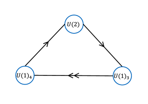
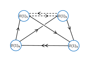
Figure 11: The left panel: $U(2)\times U(1)_{1}\times U(1)_{2}$ quiver diagram. The right panel: $U(1)_{1}\times U(1)_{2}\times U(1)_{3}\times U(1)_{4}$ quiver diagram obtained from $U(2)\to U(1)_{1}\times U(1)_{2}$ by the Higgs mechanism. The dashed quiver shows bi-fundamental scalars arising from this symmetry breaking.

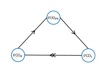
Figure 12: A quiver diagram of left-right symmetric Pati-Salam model.

We shall consider the $U(1)^{4}$ gauge theory shown in the right panel of Fig. 11. It is noted that we have two left-handed fermions charged only under $U(1)_{3}\times U(1)_{4}$, and there exist six chiral fermions and two complex scalars. This model is obtained from three nodes model of $U(2)\times U(1)_{3}\times U(1)_{4}$ in the left panel of Fig. 11 by the Higgs mechanism of $U(2)$ complex adiont scalar whose vacuum expectation value is given by $\braket{\Phi}=\mathrm{diag}(v,-v)$. This can be regard as a toy model of left-right symmetric theory obtained from the Pati-Salam model [57, 58, 59] as in Fig. 12.

The $U(1)^{4}$ model has two anomaly-free $U(1)$’s and non-trivial charged matter fields, but we focus only on the relevant gauge couplings. The detail of the anomaly cancellation is discussed in Appendix A. The divergences of $U(1)$ currents are given by

$$\partial\cdot\left(\begin{array}[]{c}j^{1}\\ j^{2}\\ j^{3}\\ j^{4}\end{array}\right)=\left(\begin{array}[]{cccc}0&0&1&-1\\ 0&0&1&-1\\ -1&-1&0&2\\ 1&1&-2&0\end{array}\right)\left(\begin{array}[]{c}Q_{1}\\ Q_{2}\\ Q_{3}\\ Q_{4}\end{array}\right),$$ (175)

and we define two independent anomaly-free $U(1)$’s with a free parameter $c$ as

$$U(1)_{X}= cU(1)_{1}+(2-c)U(1)_{2}+U(1)_{3}+U(1)_{4},$$ (176)

$$U(1)_{X^{\prime}}= \frac{3-c}{1-c}U(1)_{1}-\frac{1+c}{1-c}U(1)_{2}+U(1)_{3}+U(1)_{4}.$$ (177)

Two chiral fermions charged only under $U(1)_{3}\times U(1)_{4}$ is still neutral but other fermions have non-trivial charges under these anomaly-free $U(1)$ gauge groups. The corresponding anomaly-free gauge couplings read

$$\frac{1}{e_{X}^{2}}= \frac{c^{2}}{g_{1}^{2}}+\frac{(2-c)^{2}}{g_{2}^{2}}+\frac{1}{g_{3}^{2}}+\frac{1}{g_{4}^{2}},$$ (178)

$$\frac{1}{e_{X^{\prime}}^{2}}= \biggl{(}\frac{3-c}{1-c}\biggr{)}^{2}\frac{1}{g_{1}^{2}}+\biggl{(}\frac{1+c}{1-c}\biggr{)}^{2}\frac{1}{g_{2}^{2}}+\frac{1}{g_{3}^{2}}+\frac{1}{g_{4}^{2}}.$$ (179)

These gauge couplings are given by linear combinations of the original ones, and when $U(1)_{1}\times U(1)_{2}$ is unified to $U(2)$ we find $g_{1}=g_{2}$.

B.2 A model inspired by the SM

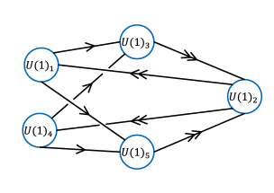
Figure 13: A diagram of quiver gauge theory inspired by the SM.

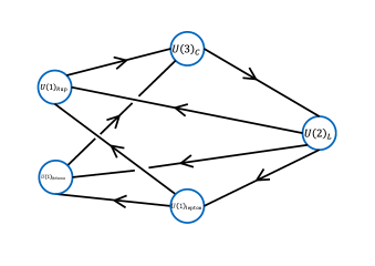
Figure 14: A quiver diagram of the SM-like model [33].

Another example is a model in Fig. 13 that is inspired by the SM-like model in Fig. 14. The divergences of chiral currents are given by

$$\partial\cdot\left(\begin{array}[]{c}j^{1}\\ j^{2}\\ j^{3}\\ j^{4}\\ j^{5}\end{array}\right)=\left(\begin{array}[]{ccccc}0&-2&1&0&1\\ 2&0&-2&2&-2\\ -1&2&0&-1&0\\ 0&-2&1&0&1\\ -1&2&0&-1&0\end{array}\right)\left(\begin{array}[]{c}Q_{1}\\ Q_{2}\\ Q_{3}\\ Q_{4}\\ Q_{5}\end{array}\right).$$ (195)

We find three anomaly-free $U(1)$’s and they can generally be written as

$$U(1)_{X}=c_{1}U(1)_{1}+U(1)_{2}+c_{2}U(1)_{3}+(2-c_{1})U(1)_{4}+(2-c_{2})U(1)_{5},$$ (196)

with two free parameters of $c_{1}$ and $c_{2}$ which will be a rational numbers. The parameters of $c_{i}$’s are taken as a gauge group is orthognal to each other. Then the fermions have non-trivial charge in this anomaly-free $U(1)$’s, but we focus only on the gauge couplings. The relavant gauge coupling is given by

$$\frac{1}{e_{X}^{2}}=\frac{c_{1}^{2}}{g_{1}^{2}}+\frac{1}{g_{2}^{2}}+\frac{c_{2}^{2}}{g_{3}^{2}}+\frac{(2-c_{1})^{2}}{g_{4}^{2}}+\frac{(2-c_{2})^{2}}{g_{5}^{2}}.$$ (197)

As mentioned earlier, an anomaly-free coupling can contain more of the original couplings as the number of $U(1)$’s in a theory increases.

Appendix C Orbifold compactification

Let us dimensionally reduce the 5D action in Eq. (100) and show the gauge couplings and Yukawa couplings in 4D. The metric of $M_{4}\times S^{1}/\mathbb{Z}_{2}$ is written by $ds_{5}^{2}=e^{-\sigma}g_{\mu\nu}dx^{\mu}dx^{\nu}+e^{2\sigma}dy^{2}$. Thus, the vielbein is given as

$$E^{A}{}_{M}=\left(\begin{array}[]{cc}e^{-\sigma/2}e^{a}{}_{\mu}&\\ &e^{\sigma}\end{array}\right),$$ (200)

where $A$ and $a$ represent 5D and 4D local Lorentz indices respectively, and $e^{a}{}_{\mu}$ is the 4D vielbein. The off-diagonal element of the vielbein is absent because the orbifold projection prohibits the graviphoton. It is noted that 5D fermion kinetic term is given by $\overline{\Psi}\Gamma^{A}E_{A}{}^{M}D_{M}\Psi$, where $E_{A}{}^{M}$ is the inverse matrix of $E^{A}{}_{M}$. Using these equations, we obtain 4D action for massless modes in Eqs. (107) and (108):

$$S_{4\mathrm{D}}=\int d^{4}x\,\sqrt{-g_{4}}\Biggl{[}\frac{\pi L}{2\kappa_{5}^{2}}\mathcal{R}_{4}-\frac{3\pi L}{4\kappa_{5}^{2}}(\partial_{\mu}\sigma)^{2}$$

$$-\frac{1}{4}\frac{\pi Le^{\sigma}}{\hat{g}_{a}^{2}}(F^{(a)}_{\mu\nu})^{2}-2\frac{1}{4}\frac{\pi Le^{\sigma}}{\hat{g}_{2}^{2}}(F^{(b)}_{\mu\nu})^{2}-\frac{1}{4}\frac{\pi Le^{\sigma}}{\hat{g}_{c}^{2}}(F^{(c)}_{\mu\nu})^{2}-2\frac{1}{4}\frac{\pi Le^{\sigma}}{\hat{g}_{2}^{2}}(F^{(d)}_{\mu\nu})^{2}-\frac{\pi Le^{-2\sigma}}{\hat{g}_{2}^{2}}|D_{\mu}\varphi|^{2}$$

$$+\pi Le^{-\sigma/2}i\overline{\psi_{ab}}{\ooalign{\hfil/\hfil\crcr$D$}}\psi_{ab}+\pi Le^{-\sigma/2}i\overline{\psi_{da}}{\ooalign{\hfil/\hfil\crcr$D$}}\psi_{da}+\pi Le^{-\sigma/2}i\overline{\psi_{cd}}{\ooalign{\hfil/\hfil\crcr$D$}}\psi_{cd}+\pi Le^{-\sigma/2}i\overline{\psi_{bc}}{\ooalign{\hfil/\hfil\crcr$D$}}\psi_{bc}$$ (209)

$$-\frac{\pi Le^{-2\sigma}}{\sqrt{2}}\varphi_{R}(\overline{\psi_{ab}^{C}}\psi_{da}+\overline{\psi_{da}}\psi_{ab}^{C})-\frac{\pi Lie^{-2\sigma}}{\sqrt{2}}\varphi_{I}(\overline{\psi_{ab}^{C}}\psi_{da}-\overline{\psi_{da}}\psi_{ab}^{C})$$

$$-\frac{\pi Le^{-2\sigma}}{\sqrt{2}}\varphi_{R}(\overline{\psi_{bc}^{C}}\psi_{cd}+\overline{\psi_{cd}}\psi_{bc}^{C})+\frac{\pi Lie^{-2\sigma}}{\sqrt{2}}\varphi_{I}(\overline{\psi_{bc}^{C}}\psi_{cd}-\overline{\psi_{cd}}\psi_{bc}^{C})-V(\sigma,\varphi)\Biggr{]},$$ (210)

where $D_{\mu}=\partial_{\mu}+i\sum_{j=a,b,c,d}q_{\psi}A^{(j)}_{\mu}$ is the covariant derivative associated with the gauge group $U(1)_{a}\times U(1)_{b}\times U(1)_{c}\times U(1)_{d}$, and the chiral fermions $\psi_{ij}$ are defined in Sec. 4.2. The four dimensional Ricci scalar is denoted by $\mathcal{R}_{4}$, and $\varphi=\varphi_{R}+i\varphi_{I}$ is the complex scalar. We introduce the scalar potential $V(\sigma,\varphi)$ formally. Thus, the gauge couplings are given as in Eq. (110).

In order to find the relation between the Yukawa coupling and the gauge coupling, we canonically normalize the fermion and the complex scalar as

$$\psi_{ij}\to\frac{e^{\sigma/4}}{\sqrt{\pi L}}\psi_{ij},\quad\varphi\to\frac{\hat{g}_{2}e^{\sigma}}{\sqrt{\pi L}}\varphi.$$ (211)

Then, the kinetic term is rewritten as

$$\pi Le^{-\sigma/2}i\overline{\psi_{ij}}{\ooalign{\hfil/\hfil\crcr$D$}}\psi_{ij}\to i\overline{\psi_{ij}}{\ooalign{\hfil/\hfil\crcr$D$}}\psi_{ij}-\frac{i}{2}\overline{\psi_{ij}}\gamma^{\mu}\psi_{ij}\partial_{\mu}\sigma.$$ (216)

Hereafter, we will ignore the derivative coupling of the radion to the fermions. The Yukawa interactions are expressed as

$$\mathcal{L}_{\mathrm{4D,Yukawa}}= -\frac{\hat{g}_{2}e^{-\sigma/2}}{\sqrt{2\pi L}}\varphi_{R}(\overline{\psi_{ab}^{C}}\psi_{da}+\overline{\psi_{da}}\psi_{ab}^{C})-\frac{\hat{g}_{2}ie^{-\sigma/2}}{\sqrt{2\pi L}}\varphi_{I}(\overline{\psi_{ab}^{C}}\psi_{da}-\overline{\psi_{da}}\psi_{ab}^{C})$$

$$-\frac{\hat{g}_{2}e^{-\sigma/2}}{\sqrt{2\pi L}}\varphi_{R}(\overline{\psi_{bc}^{C}}\psi_{cd}+\overline{\psi_{cd}}\psi_{bc}^{C})+\frac{\hat{g}_{2}ie^{-\sigma/2}}{\sqrt{2\pi L}}\varphi_{I}(\overline{\psi_{bc}^{C}}\psi_{cd}-\overline{\psi_{cd}}\psi_{bc}^{C}).$$

We introduce the Dirac fermions as

$$\psi_{a}=\left(\begin{array}[]{c}\psi_{da}\\ \psi_{ab}^{C}\end{array}\right).\quad\psi_{c}=\left(\begin{array}[]{c}\psi_{cd}\\ \psi_{bc}^{C}\end{array}\right).$$ (222)

With these Dirac fermions, the kinetic terms of the anomaly-free sector read

$$\mathcal{L}_{\mathrm{4D,KT}}= -\frac{1}{4e_{X}^{2}}\bigl{(}F^{(X)}_{\mu\nu}\bigr{)}^{2}-\frac{1}{4e_{X^{\prime}}^{2}}\bigl{(}F^{(X^{\prime})}_{\mu\nu}\bigr{)}^{2}-(\partial_{\mu}\varphi_{R})^{2}-(\partial_{\mu}\varphi_{I})^{2}$$

$$+i\overline{\psi_{a}}{\ooalign{\hfil/\hfil\crcr$\mathcal{D}$}}\psi_{a}+i\overline{\psi_{c}}{\ooalign{\hfil/\hfil\crcr$\mathcal{D}$}}\psi_{c},$$ (227)

where we neglected gauge bosons in anomalous $U(1)$’s, the anomaly-free gauge couplings are defined by Eqs. (111) and (112). As shown in Table 1, the covariant derivatives of the Dirac fermions associated with anomaly-free $U(1)$’s are expressed as

$$\mathcal{D}_{\mu}\psi_{a}= \biggl{[}\partial_{\mu}+i(-1+c)A^{(X)}_{\mu}-i\biggl{(}1+\frac{1}{c}\biggr{)}A^{(X^{\prime})}_{\mu}\biggr{]}\psi_{a},$$ (228)

$$\mathcal{D}_{\mu}\psi_{c}= \biggl{[}\partial_{\mu}-i(-1+c)A^{(X)}_{\mu}+i\biggl{(}1+\frac{1}{c}\biggr{)}A^{(X^{\prime})}_{\mu}\biggr{]}\psi_{c}.$$ (229)

The charges of $\psi_{a}$ and $\psi_{c}$ under $U(1)_{X}$ and $U(1)_{X^{\prime}}$ are opposite to each other due to the 4D anomaly-free conditions. With the Dirac spinor, the Yukawa terms in this Lagrangian are rewritten as below:

$$\mathcal{L}_{\text{4D,Yukawa}}= -ye^{-\sigma/2}\varphi_{R}\overline{\psi_{a}}\psi_{a}-iye^{-\sigma/2}\varphi_{I}\overline{\psi_{a}}\gamma_{5}\psi_{a}-ye^{-\sigma/2}\varphi_{R}\overline{\psi_{c}}\psi_{c}+iye^{-\sigma/2}\varphi_{I}\overline{\psi_{c}}\gamma_{5}\psi_{c},$$ (230)

where the 4D Yukawa coupling is defined as

$$y=\frac{\hat{g}_{2}}{\sqrt{2\pi L}}.$$ (231)

References

- [1] C. Vafa, hep-th/0509212.
- [2] H. Ooguri and C. Vafa, Nucl. Phys. B 766 (2007) 21 [hep-th/0605264].
- [3] N. Arkani-Hamed, L. Motl, A. Nicolis and C. Vafa, JHEP 0706 (2007) 060 [hep-th/0601001].
- [4] G. Obied, H. Ooguri, L. Spodyneiko and C. Vafa, arXiv:1806.08362 [hep-th].
- [5] S. K. Garg and C. Krishnan, JHEP 11 (2019), 075 [arXiv:1807.05193 [hep-th]].
- [6] H. Ooguri, E. Palti, G. Shiu and C. Vafa, Phys. Lett. B 788 (2019) 180 [arXiv:1810.05506 [hep-th]].
- [7] E. Palti, Fortsch. Phys. 67 (2019) no.6, 1900037 [arXiv:1903.06239 [hep-th]]; references therein.
- [8] C. Cheung and G. N. Remmen, Phys. Rev. Lett. 113 (2014) 051601 [arXiv:1402.2287 [hep-ph]].
- [9] E. Palti, JHEP 1708 (2017) 034 [arXiv:1705.04328 [hep-th]].
- [10] D. Lust and E. Palti, JHEP 1802 (2018) 040 [arXiv:1709.01790 [hep-th]].
- [11] E. Gonzalo and L. E. Iàñez, JHEP 1908 (2019) 118 [arXiv:1903.08878 [hep-th]].
- [12] D. Andriot, N. Cribiori and D. Erkinger, [arXiv:2004.00030 [hep-th]].
- [13] K. Benakli, C. Branchina and G. Lafforgue-Marmet, [arXiv:2004.12476 [hep-th]].
- [14] S. J. Lee, W. Lerche and T. Weigand, Nucl. Phys. B 938 (2019) 321 [arXiv:1810.05169 [hep-th]].
- [15] S. J. Lee, W. Lerche and T. Weigand, JHEP 1908 (2019) 104 [arXiv:1901.08065 [hep-th]].
- [16] B. Heidenreich, M. Reece and T. Rudelius, JHEP 1910 (2019) 055 [arXiv:1906.02206 [hep-th]].
- [17] N. Craig, I. Garcia Garcia and G. D. Kribs, [arXiv:1912.10054 [hep-ph]].
- [18] M. B. Green and J. H. Schwarz, Phys. Lett. B 149 (1984), 117-122
- [19] G. Aldazabal, L. E. Ibanez, F. Quevedo and A. Uranga, JHEP 08 (2000), 002 [arXiv:hep-th/0005067 [hep-th]].
- [20] G. Aldazabal, S. Franco, L. E. Ibanez, R. Rabadan and A. Uranga, JHEP 02 (2001), 047 [arXiv:hep-ph/0011132 [hep-ph]].
- [21] G. Aldazabal, S. Franco, L. E. Ibanez, R. Rabadan and A. Uranga, J. Math. Phys. 42 (2001), 3103-3126 [arXiv:hep-th/0011073 [hep-th]].
- [22] R. Blumenhagen, D. Lust and S. Stieberger, JHEP 0307 (2003) 036 [hep-th/0305146].
- [23] R. Blumenhagen, G. Honecker and T. Weigand, JHEP 08 (2005), 009 [arXiv:hep-th/0507041 [hep-th]].
- [24] For a review, see R. Blumenhagen, B. Kors, D. Lust and S. Stieberger, Phys. Rept. 445 (2007), 1-193 [arXiv:hep-th/0610327 [hep-th]]; references therein.
- [25] P. Saraswat, Phys. Rev. D 95 (2017) no.2, 025013 [arXiv:1608.06951 [hep-th]].
- [26] J. Polchinski, “String theory. Vol. 1: An introduction to the bosonic string” and “String theory. Vol. 2: Superstring theory and beyond.”
- [27] G. Dvali and M. Redi, Phys. Rev. D 77 (2008) 045027 [arXiv:0710.4344 [hep-th]].
- [28] N. Craig, I. Garcia Garcia and S. Koren, JHEP 1905 (2019) 140 [arXiv:1812.08181 [hep-th]].
- [29] G. Buratti, J. Calderon, A. Mininno and A. M. Uranga, arXiv:2003.09740 [hep-th].
- [30] L. E. Ibanez, F. Marchesano and R. Rabadan, JHEP 0111 (2001) 002 [hep-th/0105155].
- [31] D. Cremades, L. Ibanez and F. Marchesano, JHEP 07 (2002), 009 [arXiv:hep-th/0201205 [hep-th]].
- [32] D. Cremades, L. E. Ibanez and F. Marchesano, JHEP 0207 (2002) 022 [hep-th/0203160].
- [33] H. Verlinde and M. Wijnholt, JHEP 0701 (2007) 106 [hep-th/0508089].
- [34] M. Cvetic, J. Halverson and R. Richter, JHEP 12 (2009), 063 [arXiv:0905.3379 [hep-th]].
- [35] S. Krippendorf, M. J. Dolan, A. Maharana and F. Quevedo, JHEP 1006 (2010) 092 [arXiv:1002.1790 [hep-th]].
- [36] M. J. Dolan, S. Krippendorf and F. Quevedo, JHEP 1110 (2011) 024 [arXiv:1106.6039 [hep-th]].
- [37] M. R. Douglas and G. W. Moore, [arXiv:hep-th/9603167 [hep-th]].
- [38] A. M. Uranga, [arXiv:hep-th/0007173 [hep-th]].
- [39] B. A. Burrington, J. T. Liu and L. A. Pando Zayas, Nucl. Phys. B 747 (2006) 436 [hep-th/0602094].
- [40] For instance, see a review: M. Yamazaki, Fortsch. Phys. 56 (2008), 555-686 [arXiv:0803.4474 [hep-th]].
- [41] N. Arkani-Hamed, A. G. Cohen and H. Georgi, Phys. Rev. Lett. 86 (2001), 4757-4761 [arXiv:hep-th/0104005 [hep-th]].
- [42] H. Abe, T. Kobayashi, N. Maru and K. Yoshioka, Phys. Rev. D 67 (2003), 045019 [arXiv:hep-ph/0205344 [hep-ph]].
- [43] D. B. Costa, B. A. Dobrescu and P. J. Fox, arXiv:2001.11991 [hep-ph].
- [44] S. P. Robinson, gr-qc/0609060.
- [45] P. Anastasopoulos, M. Bianchi, E. Dudas and E. Kiritsis, JHEP 0611 (2006) 057 [hep-th/0605225].
- [46] M. Dine, N. Seiberg and E. Witten, Nucl. Phys. B 289 (1987), 589-598
- [47] H. Jockers and J. Louis, Nucl. Phys. B 705 (2005), 167-211 [arXiv:hep-th/0409098 [hep-th]].
- [48] A. Lukas, B. A. Ovrut, K. S. Stelle and D. Waldram, Nucl. Phys. B 552 (1999) 246 [hep-th/9806051].
- [49] P. Cox, T. Gherghetta and M. D. Nguyen, JHEP 2001 (2020) 188 [arXiv:1911.09385 [hep-ph]].
- [50] S. Gukov, M. Rangamani and E. Witten, JHEP 9812 (1998) 025 [hep-th/9811048].
- [51] E. Garćıa-Valdecasas, A. Mininno and A. M. Uranga, JHEP 1910 (2019) 091 [arXiv:1907.06938 [hep-th]].
- [52] T. Banks and L. J. Dixon, Nucl. Phys. B 307 (1988), 93-108
- [53] T. Banks and N. Seiberg, Phys. Rev. D 83 (2011), 084019 [arXiv:1011.5120 [hep-th]].
- [54] D. Harlow and H. Ooguri, [arXiv:1810.05338 [hep-th]].
- [55] D. Cremades, L. Ibanez and F. Marchesano, JHEP 07 (2003), 038 [arXiv:hep-th/0302105 [hep-th]].
- [56] D. Cremades, L. Ibanez and F. Marchesano, JHEP 05 (2004), 079 [arXiv:hep-th/0404229 [hep-th]].
- [57] J. C. Pati and A. Salam, Phys. Rev. D 10 (1974), 275-289
- [58] R. N. Mohapatra and J. C. Pati, Phys. Rev. D 11 (1975), 566-571
- [59] G. Senjanovic and R. N. Mohapatra, Phys. Rev. D 12 (1975), 1502