Polygonal Building Extraction by Frame Field Learning

Abstract

While state of the art image segmentation models typically output segmentations in raster format, applications in geographic information systems often require vector polygons. To help bridge the gap between deep network output and the format used in downstream tasks, we add a frame field output to a deep segmentation model for extracting buildings from remote sensing images. We train a deep neural network that aligns a predicted frame field to ground truth contours. This additional objective improves segmentation quality by leveraging multi-task learning and provides structural information that later facilitates polygonization; we also introduce a polygonization algorithm that utilizes the frame field along with the raster segmentation. Our code is available at https://github.com/Lydorn/Polygonization-by-Frame-Field-Learning.

1 Introduction

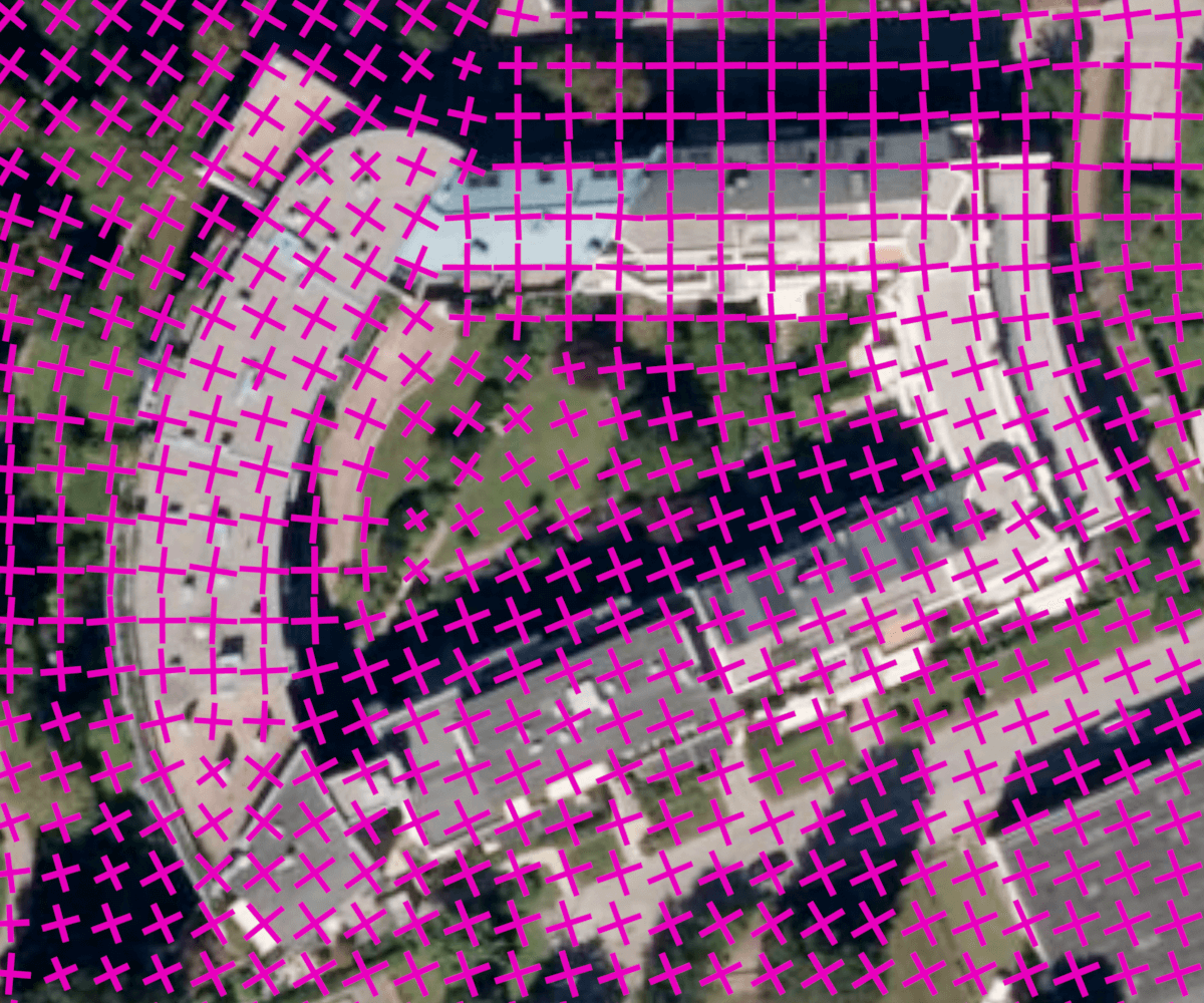
Figure 1: A frame field output by our network.

Due to their success in processing large collections of noisy images, deep convolutional neural networks (CNNs) have achieved state-of-the-art in remote sensing segmentation. Geographic information systems like Open Street Map (OSM) [30], however, require segmentation data in vector format (e.g., polygons and curves) rather than raster format, which is generated by segmentation networks. Additionally, methods that extract objects from remote sensing images require especially high throughput to handle the volume of high-resolution aerial images captured daily over large territories of land. Thus, modifications to the conventional CNN pipeline are necessary.

Existing work on deep building segmentation generally falls into one of two general categories. The first vectorizes the probability map produced by a network a posteriori, e.g., by using contour detection (marching squares [25]) followed by polygon simplification (Ramer–Douglas–Peucker [32, 13]). Such approaches suffer when the classification maps contain imperfections such as smoothed out corners, a common artifact of conventional deep segmentation methods. Moreover, as we show in Fig. 2, even perfect probability maps are challenging to polygonize due to shape information being lost from the discretization of the raster output. To improve the final polygons, these methods employ expensive and complex post-processing procedures. ASIP polygonization [20] uses polygonal partition refinement to approximate shapes from the output probability map based on a tunable parameter controlling the trade-off between complexity and fidelity. In [45], a decoder and a discriminator regularize output probability maps adversarially. This requires computing large matrices of pairwise discontinuity costs between pixels and involves adversarial training, which is less stable than conventional supervised learning.

Another category of deep segmentation methods learns a vector representation directly. For example, Curve-GCN [23] trains a graph convolutional network (GCN) to deform polygons iteratively, and PolyMapper [21] uses a recurrent neural network (RNN) to predict vertices one at a time. While these approaches directly predict polygon parameters, GCNs and RNNs suffer from several disadvantages. Not only are they more difficult to train than CNNs, but also their output topology is restricted to simple polygons without holes—a serious limitation in segmenting complex buildings. Additionally, adjoining buildings with common walls are common, especially in city centers. Curve-GCN and PolyMapper are unable to reuse the same polyline in adjoining buildings, yielding overlaps and gaps.

We introduce a building extraction algorithm that avoids the challenges above by adding a frame field output to a fully-convolutional network (see Fig. 1). While this has imperceptible effect on training or inference time, the frame field not only increases segmentation performance, e.g., yielding sharper corners, but also provides useful information for vectorization. Additional losses learn a valid frame field that is consistent with the segmentation. These losses regularize the segmentation, similar to [39], which includes MRF/CRF regularization terms in the loss function to avoid extra MRF/CRF inference steps.

The frame field allows us to devise a straightforward polygonization method extending the Active Contours Model (ACM, or “snakes”) [19], which we call the Active Skeleton Model (ASM). Rather than fitting contours to image data, ASM fits a skeleton graph, where each edge connects two junction nodes with a chain of vertices (i.e., a polyline). This allows us to reuse shared walls between adjoining buildings. To our knowledge, no existing method handles this case ([41] shows results with common walls but does not provide details). Our method naturally handles large buildings and buildings with inner holes, unlike end-to-end learning methods like PolyMapper [21]. Lastly, our polygon extraction pipeline is highly GPU-parallelizable, making it faster than more complex methods.

Our main contributions are:

1. a learned frame field aligned to object tangents, which improves segmentation via multi-task learning;

2. coupling losses between outputs for self-consistency, further leveraging multi-task learning; and

3. a fast polygonization method leveraging the frame field, allowing complexity tuning of a corner-aware simplification step and handling non-trivial topology.

2 Related work

ASIP polygonization [20] inputs an RGB image and a probability map of objects (e.g., buildings) detected in the image (e.g., by a neural network). Then, starting from a polygonal partition that oversegments the image into convex cells, the algorithm refines the partition while labeling its cells by semantic class. The refinement process is an optimization with terms that balance fidelity to the input against complexity of the output polygons. The configuration space is explored by splitting and merging the polygonal cells. As the fidelity and complexity terms can be balanced with a coefficient, the fidelity-to-complexity ratio can be tuned. However, there does not exist a systematic approach for interpreting or determining this coefficient. While ASIP post-processes the output of a deep learning method, recent approaches aim for an end-to-end pipeline.

CNNs are successful at converting grid-based input to grid-based output for tasks where each output pixel depends on its local neighborhood in the input. In this setting, it is straightforward and efficient to train a network for supervised prediction of segmentation probability maps. The paragraphs below, however, detail major challenges when using such an approach to extract polygonal buildings.

First, the model needs to produce variable-sized outputs to capture varying numbers of objects, contours, and vertices. This requires complex architectures like recurrent neural networks (RNNs) [18], which are not as efficiently trained as CNNs and need multiple iterations at inference time. Such is the case for PolyMapper [21], Polygon-RNN [5], and Polygon-RNN++ [1]. Curve-GCN [23] predicts a fixed number of vertices simultaneously.

A second challenge is that the model must make discrete decisions of whether to add a contour, whether to add a hole to an object, and with how many vertices to describe a contour. Adding a contour is solved by object detection: a contour is predicted for each detected object. Adding holes to an object is more challenging, but a few methods detect holes and predict their contours. One model, BSP-Net [8], circumvents this issue by combining predicted convex shapes for the final output, producing shapes in a compact format, with potential holes inside. To our knowledge, the number of vertices is not a variable that current deep learning models can optimize for; discrete decisions are difficult to pose differentiably without training techniques such as the straight-through estimator [3] or reinforcement learning [37, 28, 27].

A third challenge is that, unlike probability maps, the output structure of polygonal building extraction is not grid-like. Within the network, the grid-like structure of the image input has to be transformed to a more general planar graph structure representing building outlines. City centers have the additional problem of adjoining buildings that share a wall. Ideally, the output geometry for such a case would be a collection of polygons, one for each individual building, which share polylines corresponding to common walls. Currently, no existing deep learning method tackles this case. Our method solves it but is not end-to-end. PolyMapper [21] tackles the individual building and road network extraction tasks. As road networks are graphs, they propose a novel sequentialization method to reformulate graph structures as closed polygons. Their approach might work in the case of adjoining buildings with common walls. Their output structure, however, is less adapted to GPU computation, making it less efficient. RNNs such as PolyMapper [21], Polygon-RNN [5], and Polygon-RNN++ [1] perform beam search at inference to prune off improbable sequences, which requires more vertex predictions than are used in the final output and is inefficient. The DefGrid [14] module is a non-RNN approach where the network processes polygonal superpixels. It is more complex than our simple fully-convolutional network and is still subject to the rounded corner problem.

The challenges above demand a middle ground between learning a bitmap segmentation followed by a hand-crafted polygonization method and end-to-end methods, aiming to be easily-deployable, topologically flexible w.r.t. holes and common walls, and efficient. A step in this direction is the machine-learned building polygonization [44] that predicts building segmentations using a CNN, uses a generative adversarial network to regularize building boundaries, and learns a building corner probability map, from which vertices are extracted. In contrast, our model predicts a frame field both as additional geometric information (instead of a building corner probability map) and as a way to regularize building boundaries (instead of adversarial training). The addition of this frame field output is similar in spirit to DiResNet [12], a road extraction neural network that outputs road direction in addition to road segmentation, first introduced in [2]. The orientation is learned for each road pixel by a cross-entropy classification loss whose labels are orientation bins. This additional geometric feature learned by the network improves the overall geometric integrity of the extracted objects (in their case road connectivity). The differences to our method include the following: (1) our frame fields encode two orientations instead of one (needed for corners), (2) we use a regression loss instead of a classification loss, and (3) we use coupling losses to promote coherence between segmentation and frame field.

3 Method

Our key idea is to help the polygonization method solve ambiguous cases caused by discrete probability maps by asking the neural network to output missing shape information in the form of a frame field (see Fig. 2). This practically does not increase training and inference time, allows for simpler and faster polygonization, and regularizes the segmentation—solving the problem of small misalignments of the ground truth annotations that yield rounded corners if no regularization is used.

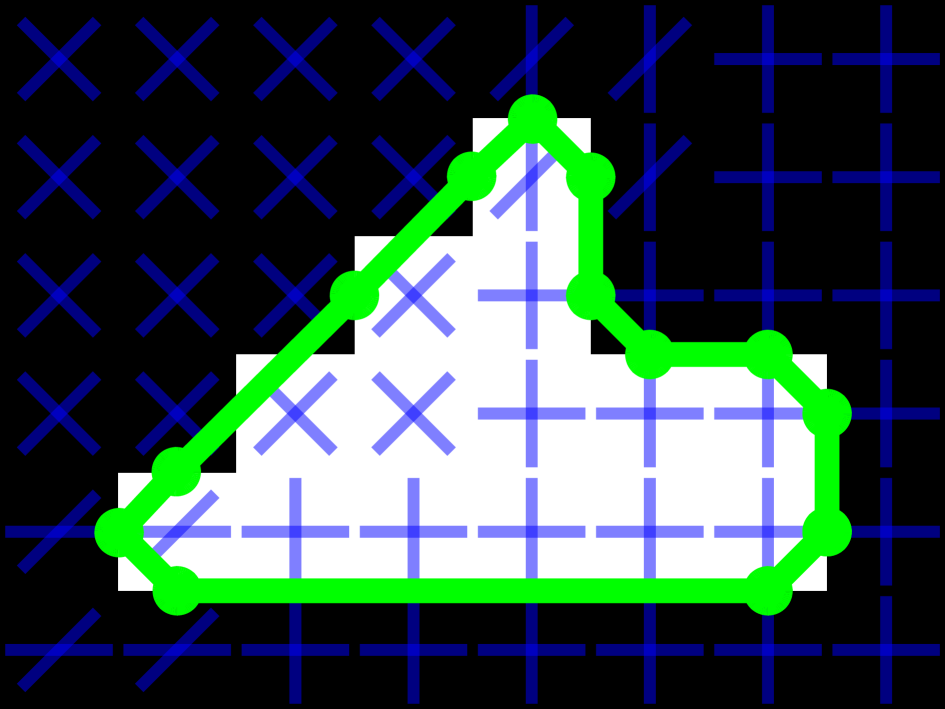
(a) Iter. 0

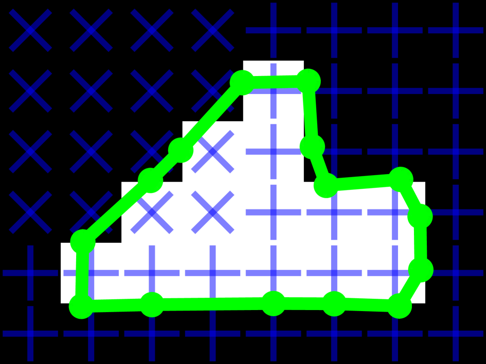
(b) Iter. 50

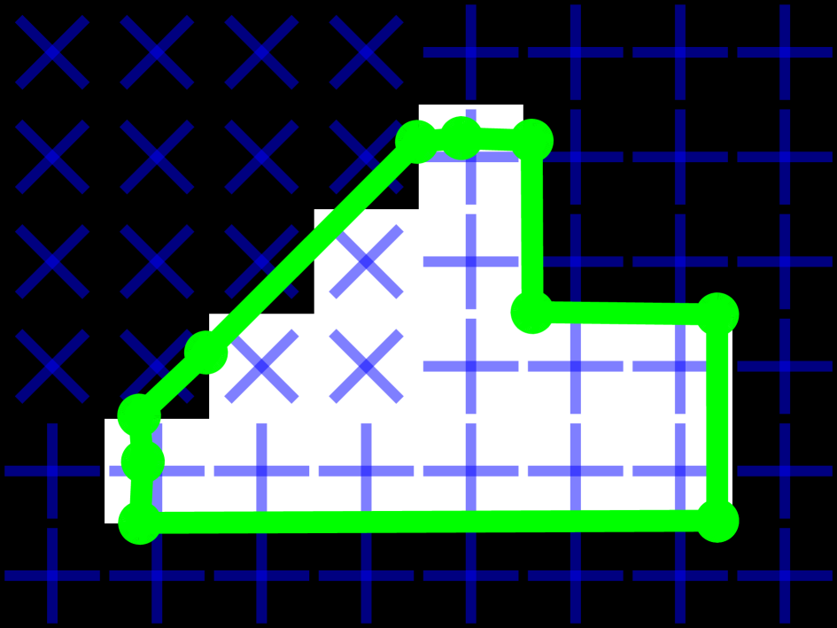
(c) Iter. 250

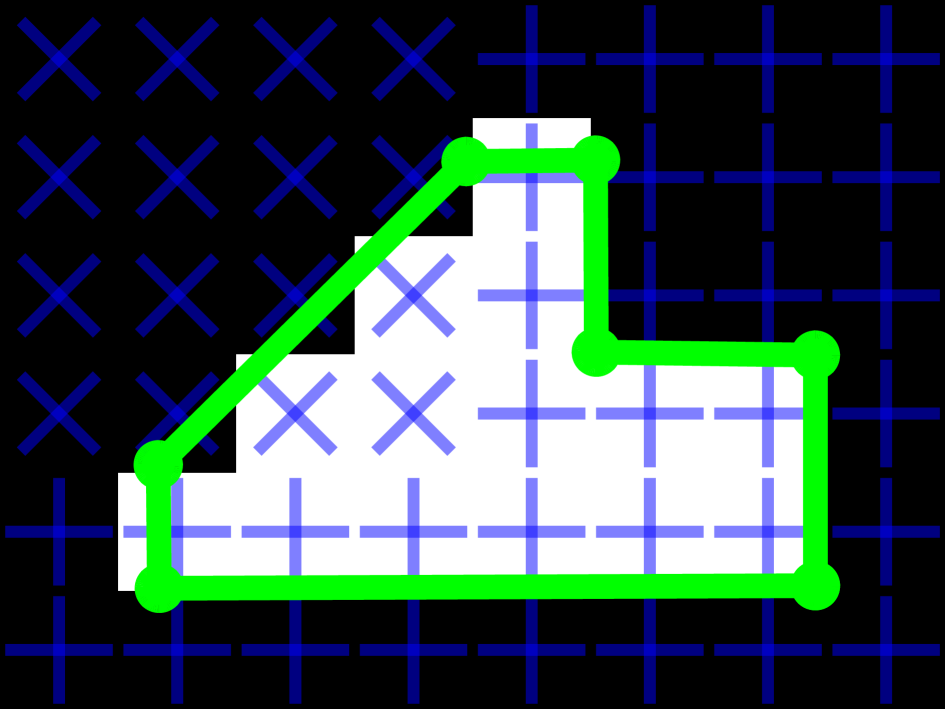
(d) Result

Figure 2: Even a perfect classification map can yield incorrect polygonization due to a locally ambiguous probability map, as shown in (a), the output of marching squares. Our polygonization method iteratively optimizes the contour (b-d) to align to a frame field, yielding better results as our frame field (blue) disambiguates between slanted walls and corners, preventing corners from being cut off.

3.1 Frame fields

We provide the necessary background on frame fields, a key part of our method. Following [42, 11], a frame field is a 4-PolyVector field, which assigns four vectors to each point of the plane. In the case of a frame field, however, the first two vectors are constrained to be opposite to the other two, i.e., each point is assigned a set of vectors $\{u,-u,v,-v\}$. At each point in the image, we consider the two directions that define the frame as two complex numbers $u,v\in\mathbb{C}$. We need two directions (rather than only one) because buildings, unlike organic shapes, are regular structures with sharp corners, and capturing directionality at these sharp corners requires two directions. To encode the directions in a way that is agnostic to relabeling and sign change, we represent them as coefficients of the following polynomial:

$$f(z)=(z^{2}-u^{2})(z^{2}-v^{2})=z^{4}+c_{2}z^{2}+c_{0}\,.$$ (1)

We denote (1) above by $f(z;c_{0},c_{2})$. Given a $(c_{0},c_{2})$ pair, we can easily recover one pair of directions defining the corresponding frame:

$$\left\{\begin{aligned} c_{0}&=u^{2}v^{2}\\ c_{2}&=-(u^{2}+v^{2})\end{aligned}\right.\iff\left\{\begin{aligned} u^{2}&=-\tfrac{1}{2}\left(c_{2}+\sqrt{c_{2}^{2}-4c_{0}}\right)\\ v^{2}&=-\tfrac{1}{2}\left(c_{2}-\sqrt{c_{2}^{2}-4c_{0}}\right)\,.\end{aligned}\right.$$ (2)

In our approach, inspired by [4], we learn a smooth frame field with the property that, along building edges, at least one field direction is aligned to the polygon tangent direction. At polygon corners, the field aligns to both tangent directions, motivating our use of PolyVector fields rather than vector fields. Away from polygon boundaries, the frame field does not have any alignment constraints but is encouraged to be smooth and not collapse to a line field. Like [4], we formulate the field computation variationally, but, unlike their approach, we use a neural network to learn the field at each pixel, which is also explored in [38]. To avoid sign and ordering ambiguity, we learn a $(c_{0},c_{2})$ pair per pixel rather than $(u,v)$.

3.2 Frame field learning

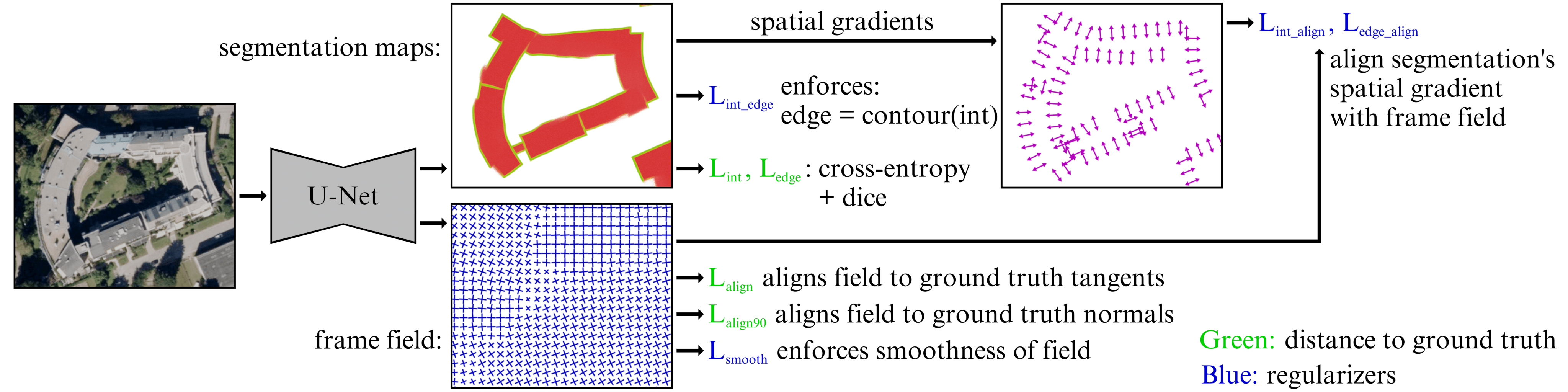
Figure 3: Given an overhead image, our model outputs an edge mask, interior mask, and frame field. The loss aligns the masks and field to ground truth data, enforces smoothness of the frame field, and ensures consistency between the outputs.

We describe our method, illustrated in Fig. 3. Our network takes a $3\!\times\!H\!\times\!W$ image $I$ as input and outputs a pixel-wise classification map and a frame field. The classification map contains two channels, $\widehat{y}_{\textit{int}}$ corresponding to building interiors and $\widehat{y}_{\textit{edge}}$ to building boundaries. The frame field contains four channels corresponding to the two complex coefficients $\widehat{c}_{0},\widehat{c}_{2}\in\mathbb{C}$, as in §3.1 above.

Segmentation losses.

Our method can be used with any deep segmentation model as a backbone; in our experiments, we use the U-Net [33] and DeepLabV3 [7] architectures. The backbone outputs an $F$-dimensional feature map $\widehat{y}_{\textit{backbone}}\in\mathbb{R}^{F\times H\times W}$. For the segmentation task, we append to the backbone a fully-convolutional block (taking $\widehat{y}_{\textit{backbone}}$ as input) consisting of a $3\!\times\!3$ convolutional layer, a batch normalization layer, an ELU nonlinearity, another $3\!\times\!3$ convolution, and a sigmoid nonlinearity. This segmentation head outputs a segmentation map $\widehat{y}_{\textit{seg}}\in\mathbb{R}^{2\times H\times W}$. The first channel contains the object interior segmentation map $\widehat{y}_{\textit{int}}$ and the second contains the contour segmentation map $\widehat{y}_{\textit{edge}}$. Our training is supervised—each input image is labeled with ground truth $y_{\textit{int}}$ and $y_{\textit{edge}}$, corresponding to rasterized polygon interiors and edges, respectively. We then use a linear combination of the cross-entropy loss and Dice loss [36] for loss $L_{\textit{int}}$ applied on the interior output as well as loss $L_{\textit{edge}}$ applied on the contour (edge) output.

Frame field losses.

In addition to the segmentation masks, our network outputs a frame field. We append another head to the backbone via a fully-convolutional block consisting of a $3\!\times\!3$ convolutional layer, a batch normalization layer, an ELU nonlinearity, another $3\!\times\!3$ convolution, and a tanh nonlinearity. This frame field block inputs the concatenation of the output features of the backbone and the segmentation output: $[\widehat{y}_{\textit{backbone}},\widehat{y}_{\textit{seg}}]\in\mathbb{R}^{(F+2)\times H\times W}$. It outputs the frame field with $\widehat{c}_{0},\widehat{c}_{2}\in\mathbb{C}^{H\times W}$. The corresponding ground truth label is an angle $\theta_{\tau}\in[0,\pi)$ of the unsigned tangent vector of the polygon contour. We use three losses to train the frame field:

$$L_{\textit{align}} =\tfrac{1}{HW}\sum_{{x}\in I}y_{\textit{edge}}({x})|f(e^{i\theta_{\tau}};\widehat{c}_{0}({x}),\widehat{c}_{2}({x}))|^{2},$$ (3)

$$L_{\textit{align90}} =\tfrac{1}{HW}\sum_{{x}\in I}y_{\textit{edge}}({x})|f(e^{i\theta_{\tau^{\bot}}};\widehat{c}_{0}({x}),\widehat{c}_{2}({x}))|^{2},$$ (4)

$$L_{\textit{smooth}} =\tfrac{1}{HW}\sum_{{x}\in I}\left(\|\nabla\widehat{c}_{0}({x})\|^{2}+\|\nabla\widehat{c}_{2}({x})\|^{2}\right),$$ (5)

where $\theta_{w}$ is the direction of $w$ ($w=\|w\|_{2}e^{i\theta_{w}}$), and $\tau^{\bot}=\tau-\tfrac{\pi}{2}$. Each loss measures a different property of the field:

• $L_{\textit{align}}$ enforces alignment of the frame field to the tangent directions. This term is small when the polynomial $f(\cdot;\widehat{c}_{0},\widehat{c}_{2})$ has a root near $e^{i\theta_{\tau}}$, implicitly implying that one of the field directions $\{\pm u,\pm v\}$ is aligned with the tangent direction $\tau$. Since (1) has no odd-degree terms, this term has no dependence on the sign of $\tau$, as desired.

• $L_{\textit{align90}}$ prevents the frame field from collapsing to a line field by encouraging it to also align with $\tau^{\bot}$.

• $L_{\textit{smooth}}$ is a Dirichlet energy measuring the smoothness of $\widehat{c}_{0}({x})$ and $\widehat{c}_{2}({x})$ as functions of location ${x}$ in the image. Smoothly-varying $\widehat{c}_{0}$ and $\widehat{c}_{2}$ yield a smooth frame field.

Output coupling losses.

We add coupling losses to ensure mutual consistency between our network outputs:

$$L_{\textit{int align}} =\frac{1}{HW}\sum_{{x}\in I}f(\nabla\widehat{y}_{\textit{int}}({x});\widehat{c}_{0}({x}),\widehat{c}_{2}({x}))^{2},$$ (6)

$$L_{\textit{edge align}} =\frac{1}{HW}\sum_{{x}\in I}f(\nabla\widehat{y}_{\textit{edge}}({x});\widehat{c}_{0}({x}),\widehat{c}_{2}({x}))^{2},$$ (7)

$$\begin{split}L_{\textit{int edge}}&=\frac{1}{HW}\sum_{{x}\in I}\max\left(1-\widehat{y}_{\textit{int}}({x}),\|\nabla\widehat{y}_{\textit{int}}({x})\|_{2}\right)\\ &\cdot\left|\|\nabla\widehat{y}_{\textit{int}}({x})\|_{2}-\widehat{y}_{\textit{edge}}({x})\right|.\end{split}$$ (8)

• $L_{\textit{int align}}$ aligns the spatial gradient of the predicted interior map $\widehat{y}_{\textit{int}}$ with the frame field (analogous to (3)).

• $L_{\textit{edge align}}$ aligns the spatial gradient of the predicted edge map $\widehat{y}_{\textit{edge}}$ with the frame field (analogous to (3)).

• $L_{\textit{int edge}}$ makes the predicted edge map be equal to the norm of the spatial gradient of the predicted interior map. This loss is applied outside of buildings (hence the $1-\widehat{y}_{\textit{int}}({x})$ term) and along building contours (hence the $\|\nabla\widehat{y}_{\textit{int}}({x})\|_{2}$ term) and is not applied inside buildings, so that common walls between adjoining buildings can still be detected by the edge map.

Final loss.

Because the losses ($L_{\textit{int}}$, $L_{\textit{edge}}$, $L_{\textit{align}}$, $L_{\textit{align90}}$, $L_{\textit{smooth}}$, $L_{\textit{int align}}$, $L_{\textit{edge align}}$, and $L_{\textit{int edge}}$) have distinct units, we compute a normalization coefficient for each loss by averaging its value over a random subset of the training dataset using a randomly-initialized network. Losses are then normalized by this coefficient before being linearly combined. This normalization aims to rescale losses such that they are easier to balance. More details are in the supplementary materials.

3.3 Frame field polygonization

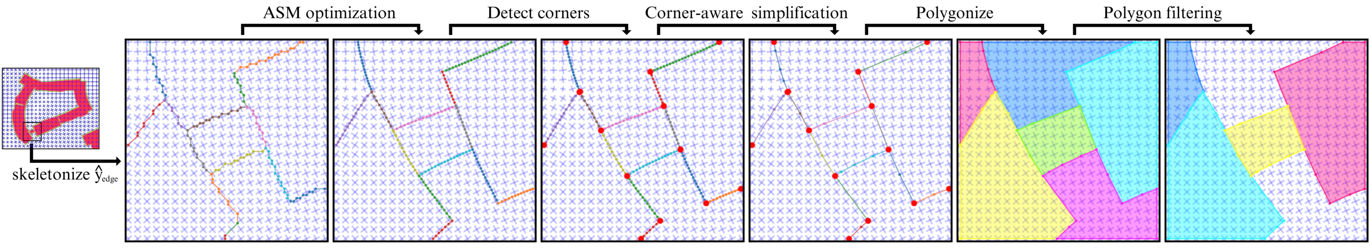
Figure 4: Overview of our post-processing polygonization algorithm. Given an interior classification map and frame field (Fig. 3) as input, we optimize the contour to align to the frame field using an Active Skeleton Model (ASM) and detect corners using the frame field, simplifying non-corner vertices.

The main steps of our polygonization method are shown in Fig. 4. It is inspired by the Active Contour Model (ACM) [19]. ACM is initialized with a given contour and minimizes an energy function $E_{\textit{contour}}^{*}$, which moves the contour points toward an optimal position. Usually this energy is composed of a term to fit the contour to the image and additional terms to limit the amount of stretch and/or curvature. The optimization is performed by gradient descent. Overall the ACM lends itself perfectly for parallelized execution on the GPU, and the optimization can be performed using an automatic differentiation module included in deep learning frameworks. We adapt ACM so that the optimization is performed on a skeleton graph instead of contours, giving us the Active Skeleton Model (ASM). We call the skeleton graph the graph of connected pixels of the skeleton image obtained by the thinning method [43] applied on the building wall probability map $y_{\textit{edge}}$. The following energy terms are used:

• $E_{\textit{probability}}$ fits the skeleton paths to the contour of the building interior probability map $y_{\textit{int}}({v})$ at a certain probability threshold $\ell$ (set to 0.5 in practice).

• $E_{\textit{frame field align}}$ aligns each edge of the skeleton graph to the frame field.

• $E_{\textit{length}}$ ensures that the node distribution along paths remains homogeneous as well as tight.

Details about our data structure (designed for GPU computation), definition and computation of our energy terms, and explanation of our corner-aware simplification step can be found in the supplementary materials.

4 Experimental setup

4.1 Datasets

Our method requires ground truth polygonal building annotations (rather than raster binary masks) so that the ground truth angle for the frame field can be computed by rasterizing separately each polygon edge and taking the edge’s angle. Thus, for each pixel we get a $\theta_{\tau}$ value, which is used in $L_{\textit{align}}$.

We perform experiments on these datasets (more details in the supplementary material):

• CrowdAI Mapping Challenge dataset [34] (CrowdAI dataset): 341438 aerial images of size $300\!\times\!300$ pixels with associated ground truth polygonal annotations.

• Inria Aerial Image Labeling dataset [26] (Inria dataset): 360 aerial images of size $5000\!\times\!5000$ pixels. Ten cities are represented, making it more varied than the CrowdAI dataset. However, the ground truth is in the form of raster binary masks. We thus create the Inria OSM dataset by taking OSM polygon annotations and correcting their misalignment using [15]. We also create the Inria Polygonized dataset by converting the original ground truth binary masks to polygon annotations with our polygonization method (see supplementary materials).

• Private dataset: 57 satellite images for training with sizes varying from $2000\!\times\!2000$ pixels to $20000\!\times\!20000$ pixels, captured over 30 different cities from all continents with three different types of satellites. This is our most varied and challenging dataset. However, the building outline polygons were manually labeled precisely by an expert, ensuring the best possible ground truth. Results for this private dataset are in the supplementary material.

4.2 Backbones

The first backbone we use is U-Net16, a small U-Net [33] with 16 starting hidden features (instead of 64 in the original). We also use DeepLab101, a DeepLabV3 [7] model that utilizes a ResNet-101 [17] encoder. Our best performing model is UResNet101—a U-Net with a ResNet-101 [17] encoder (pre-trained on ImageNet [10]). We observed that the pre-trained ResNet-101 encoder achieves better final performance than random initialization. For the UResNet101, we additionally use distance weighting for the cross-entropy loss, as done for the original U-Net [33].

4.3 Ablation study and additional experiments

We perform an ablation study to validate various components of our method (results in Tables 1,  2, and  4):

• “No field” removes the frame field output for comparison to pure segmentation. Only interior segmentation $L_{\textit{int}}$, edge segmentation $L_{\textit{edge}}$ and interior/edge coupling $L_{\textit{int edge}}$ losses remain.

• “Simple poly.” uses a baseline polygonization algorithm (marching-squares contour detection followed by the Ramer–Douglas–Peucker simplification) on the interior classification map learned by our full method. This allows us to study the improvement of our polygonization method from leveraging the frame field.

Additional experiments in the supplementary material include: “no coupling losses” removes all coupling losses ($L_{\textit{int align}}$, $L_{\textit{edge align}}$, $L_{\textit{int edge}}$) to determine whether enforcing consistency between outputs has an impact; “no $L_{\textit{align90}}$,” “no $L_{\textit{int edge}}$,” “no $L_{\textit{int align}}$ and $L_{\textit{edge align}}$,” and “no $L_{\textit{smooth}}$” all remove the specified losses; “complexity vs. fidelity” varies the simplification tolerance parameter $\varepsilon$ to demonstrate the trade-off between complexity and fidelity of our corner-aware simplification procedure.

4.4 Metrics

The standard metric for image segmentation is Intersection over Union (IoU), which is then used to compute other metrics such as MS COCO [22], Average Precision (AP), and Average Recall (AR)—along with variants AP${}_{50}$, AP${}_{75}$, AR${}_{50}$, AR${}_{75}$. Since we aim to produce clean geometry, it is important to measure contour regularity, not captured by the area-based metrics IoU, AP, and AR. Moreover, as annotations are bound to have some alignment noise, only optimizing IoU will favor blurry segmentations with rounded corners over sharp segmentations, as the blurry ones correspond to the shape expectation of the noisy ground truth annotation; segmentation results with sharp corners may even yield a lower IoU than segmentations with rounded corners. We thus introduce the max tangent angle error metric that compares the tangent angles between predicted polygons and ground truth annotations, penalizing contours not aligned with the ground truth. It is computed by uniformly sampling points along a predicted contour, computing the angle of the tangent for each point, and comparing it to the tangent angle of the closest point on the ground truth contour. The max tangent angle error is the maximum tangent angle error over all sampled points. More details about the computation of these metrics can be found in the supplementary material.

5 Results and discussion

5.1 CrowdAI dataset

U-Net variant + ASIP p

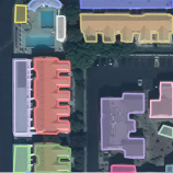
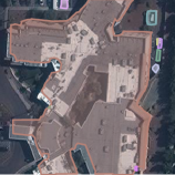
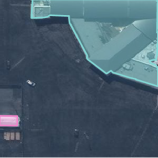
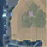
PolyMapper

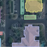
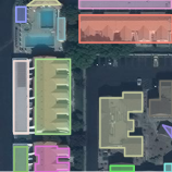
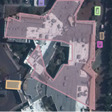
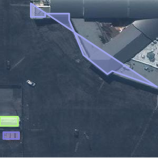
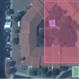
Ours p

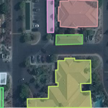
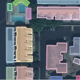
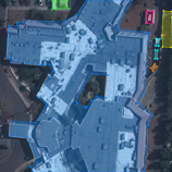
Figure 5: Example building extraction results on CrowdAI test images. Buildings become more complex from left to right. (top) U-Net variant [9] + ASIP [20], (middle) PolyMapper [21], and (bottom) ours: UResNet101 (full), frame field polygonization.

We visualize our polygon extraction results for the CrowdAI dataset and compare them to other methods in Fig. 5. The ASIP polygonization method [20] inputs the probability maps of a U-Net variant [9] that won the CrowdAI challenge. All methods perform well on common building types, e.g., houses and residential buildings, but we can see that results of ASIP are less regular than PolyMapper and ours. For more complex building shapes (e.g., not rectangular or with a hole inside), ASIP outputs reasonable results, albeit still not very regular. However, the PolyMapper approach of object detection followed by polygonal outline regression does not work in the most difficult cases. It does not support nontrivial topology by construction, but also, it struggles with large complex buildings. We hypothesize that PolyMapper suffers from the fact that there are not many complex buildings and does not generalize as well as fully-convolutional networks.

We report results on the original validation set of the CrowdAI dataset for the max tangent angle error in Table 1 and MS COCO metrics in Table 2. “(with field)” refers to models trained with our full frame field learning method, “(no field)” refers to models trained without any frame field output, “mask” refers to the output raster segmentation mask of the network, “our poly.” refers to our frame field polygonization method, and “simple poly.” refers to the baseline polygonization of marching squares followed by Ramer-Douglas-Peucker simplification. We also applied our polygonization method to the same probability maps used by the ASIP polygonization method (U-Net variant [9]) for fair comparison of polygonization methods.

In Table 1, “simple poly.” performs better using “(with field)” segmentation compared to “(no field)” because of a regularization effect from frame field learning. PolyMapper performs significantly better than “simple poly.” even though it is not explicitly regularized. Our frame field learning and polygonization method is necessary to decrease the error further and compare favorably to PolyMapper.

Method	Mean max tangent angle errors $\downarrow$
UResNet101 (no field), simple poly.	51.9°
UResNet101 (with field), simple poly.	45.1°
U-Net variant [9], ASIP poly. [20]	44.0°
UResNet101 (with field), ASIP poly. [20]	38.3°
U-Net variant [9], UResNet101 our poly.	36.6°
PolyMapper [21]	33.1°
UResNet101 (with field), our poly.	31.9°

Table 1: Mean max tangent angle errors over all the original validation polygons of the CrowdAI dataset [34].

In Table 2, our UResNet101 (with field) outperforms most previous works, except “U-Net variant [9], ASIP poly. [20]” due to the U-Net variant being the winning entry to the challenge. However our polygonization applied after that same U-Net variant achieves better max tangent angle error and AP than ASIP but worse AR. The same is true when applying ASIP to our UResNet101 (with field): it has slightly worse AP, AR, and max tangent angle error. However, the ASIP method also results in better max tangent angle error when using our UResNet101 (with field) compared to using the U-Net variant.

Method	$AP$ $\uparrow$	$AP_{50}$ $\uparrow$	$AP_{75}$ $\uparrow$	$AR$ $\uparrow$	$AR_{50}$ $\uparrow$	$AR_{75}$ $\uparrow$
UResNet101 (no field), mask	62.4	86.7	72.7	67.5	90.5	77.4
UResNet101 (no field), simple poly.	61.1	87.4	71.2	64.7	89.4	74.1
UResNet101 (with field), mask	64.5	89.3	74.6	68.1	91.0	77.7
UResNet101 (with field), simple poly.	61.7	87.7	71.5	65.4	89.9	74.6
UResNet101 (with field), our poly.	61.3	87.5	70.6	65.0	89.4	73.9
UResNet101 (with field), ASIP poly. [20]	60.0	86.3	69.9	64.0	88.8	73.4
U-Net variant [9], UResNet101 our poly.	67.0	92.1	75.6	73.2	93.5	81.1
Mask R-CNN [16] [35]	41.9	67.5	48.8	47.6	70.8	55.5
PANet [24]	50.7	73.9	62.6	54.4	74.5	65.2
PolyMapper [21]	55.7	86.0	65.1	62.1	88.6	71.4
U-Net variant [9], ASIP poly. [20]	65.8	87.6	73.4	78.7	94.3	86.1

Table 2: AP and AR results on the CrowdAI dataset [34] for all polygonization experiments.

Method	Time (sec) $\downarrow$	Hardware
PolyMapper [21]	0.38	GTX 1080Ti
ASIP [20]	0.15	Laptop CPU
Ours	0.04	GTX 1080Ti

Table 3: Average times to extract buildings from a $300\!\times\!300$ pixel patch. Ours refers to UResNet101 (with field), our poly. ASIP’s time does not include model inference.

Runtimes.

We compare runtimes in Table 3. ASIP does not have a GPU implementation. In their paper they give an average runtime of 1-3s on CPU with ~10% CPU utilization. Assuming perfect parallelization, they estimate their average runtime to be 0.15s with 100% CPU utilization. Their method uses a priority queue for optimizing the polygonal partitioning with various geometric operators and is harder to implement on GPU. Our efficient data structure makes our building extraction competitive with prior work.

5.2 Inria OSM dataset

U-Net16 (no field), simple poly.

U-Net16 (with field), our poly.

Figure 6: Small crop of Inria dataset results.

The Inria OSM dataset is more challenging than the CrowdAI dataset because it contains more varied areas (e.g., countryside, city center, residential, and commercial) with different building types. It also contains adjacent buildings with common walls, which our edge segmentation output can detect. The mean IoU on test images of the output classification maps is 78.0% for the U-Net16 trained with a frame field compared to 76.9% for the U-Net16 with no frame field. The IoU does not significantly penalize irregular contours, but, by visually inspecting segmentation outputs as in Fig. 6, we can see the effect of the regularization. Our method successfully handles complex building shapes which can be very large, with blocks of buildings featuring common walls and holes. See the supplementary materials for more results.

5.3 Inria polygonized dataset

Eugene Khvedchenya¹, simple poly.

UResNet101 (with field), our poly.

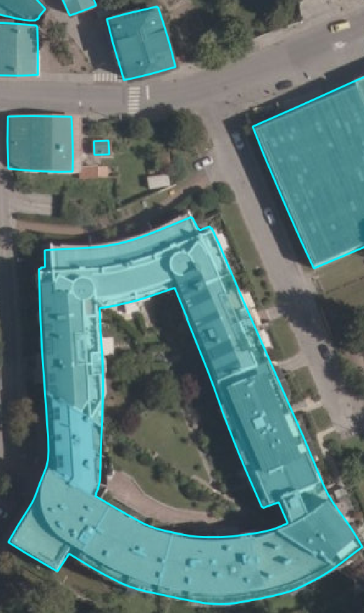
Figure 7: Crop of an Inria polygonized dataset test image.

Method	mIoU $\uparrow$	Mean max tangent angle errors $\downarrow$
Eugene Khvedchenya1, simple poly.	80.7%	52.2 °
ICTNet [6], simple poly.	80.1%	52.1°
UResNet101 (no field), simple poly.	73.2%	52.0°
Zorzi et al. [44] poly.	74.4%	34.5°
UResNet101 (with field), our poly.	74.8%	28.1°

Table 4: IoU and mean max tangent angle errors for polygon extraction methods on the Inria polygonized dataset.

The Inria polygonized dataset with its associated challenge allows us to directly compare to other methods trained on the same ground truth, even though it does not consider learning of separate buildings. In Table 4, our method matches [44] in terms of mIoU, with lower max tangent angle error. The two top methods on the leaderboard (ICTNet [6] and “Eugene Khvedchenya”) achieve a mIoU over 80%, but they lack contour regularity with high max tangent angle error; they also only output segmentation masks, needing a posteriori polygonization to extract polygonal buildings. Fig. 7 shows the cleaner geometry of our method. The ground truth of the Inria polygonized dataset has misalignment noise, yielding imprecise corners that produce rounded corners in the prediction if no regularization is applied. See the supplementary materials for more results.

6 Conclusion

We improve on the task of building extraction by learning an additional output to a standard segmentation model: a frame field. This motivates the use of a regularization loss, leading to more regular contours, e.g., with sharp corners. Our approach is efficient since the model is a single fully-convolutional network. The training is straightforward, unlike adversarial training, direct shape regression, and recurrent networks, which require significant tuning and more computational power. The frame field adds virtually no cost to inference time, and it disambiguates tough polygonization cases, making our polygonization method less complex. Our data structure for the polygonization makes it parallelizable on the GPU. We handle the case of holes in buildings as well as common walls between adjoining buildings. Because of the skeleton graph structure, common wall polylines are naturally guaranteed to be shared by the buildings on either side. As future work, we could apply our method to any image segmentation network, including multi-class segmentation, where the frame field could be shared between all classes.

7 Acknowledgements

Thanks to ANR for funding the project EPITOME ANR-17-CE23-0009 and to Inria Sophia Antipolis - Méditerranée “Nef” computation cluster for providing resources and support. The MIT Geometric Data Processing group acknowledges the generous support of Army Research Office grant W911NF2010168, of Air Force Office of Scientific Research award FA9550-19-1-031, of National Science Foundation grant IIS-1838071, from the CSAIL Systems that Learn program, from the MIT–IBM Watson AI Laboratory, from the Toyota–CSAIL Joint Research Center, from a gift from Adobe Systems, from an MIT.nano Immersion Lab/NCSOFT Gaming Program seed grant, and from the Skoltech–MIT Next Generation Program. This work was also supported by the National Science Foundation Graduate Research Fellowship under Grant No. 1122374.

Supplementary Materials

Contents

1. 1 Introduction
2. 2 Related work
3. 3 Method
   1. 3.1 Frame fields
   2. 3.2 Frame field learning
   3. 3.3 Frame field polygonization
4. 4 Experimental setup
   1. 4.1 Datasets
   2. 4.2 Backbones
   3. 4.3 Ablation study and additional experiments
   4. 4.4 Metrics
5. 5 Results and discussion
   1. 5.1 CrowdAI dataset
   2. 5.2 Inria OSM dataset
   3. 5.3 Inria polygonized dataset
6. 6 Conclusion
7. 7 Acknowledgements
8. 1 Frame field learning details
   1. 1.1 Model architecture
   2. 1.2 Losses
   3. 1.3 Handling numerous heterogeneous losses
   4. 1.4 Training details
9. 2 Frame field polygonization details
   1. 2.1 Data structure
   2. 2.2 Active Skeleton Model
   3. 2.3 Corner-aware polygon simplification

1 Frame field learning details

1.1 Model architecture

We show in Fig. S1 how we add a frame field output to an image segmentation backbone. The backbone can be any (possibly pretrained) network as long as it outputs an $F$-dimensional feature map $\widehat{y}_{\textit{backbone}}\in\mathbb{R}^{F\times H\times W}$.

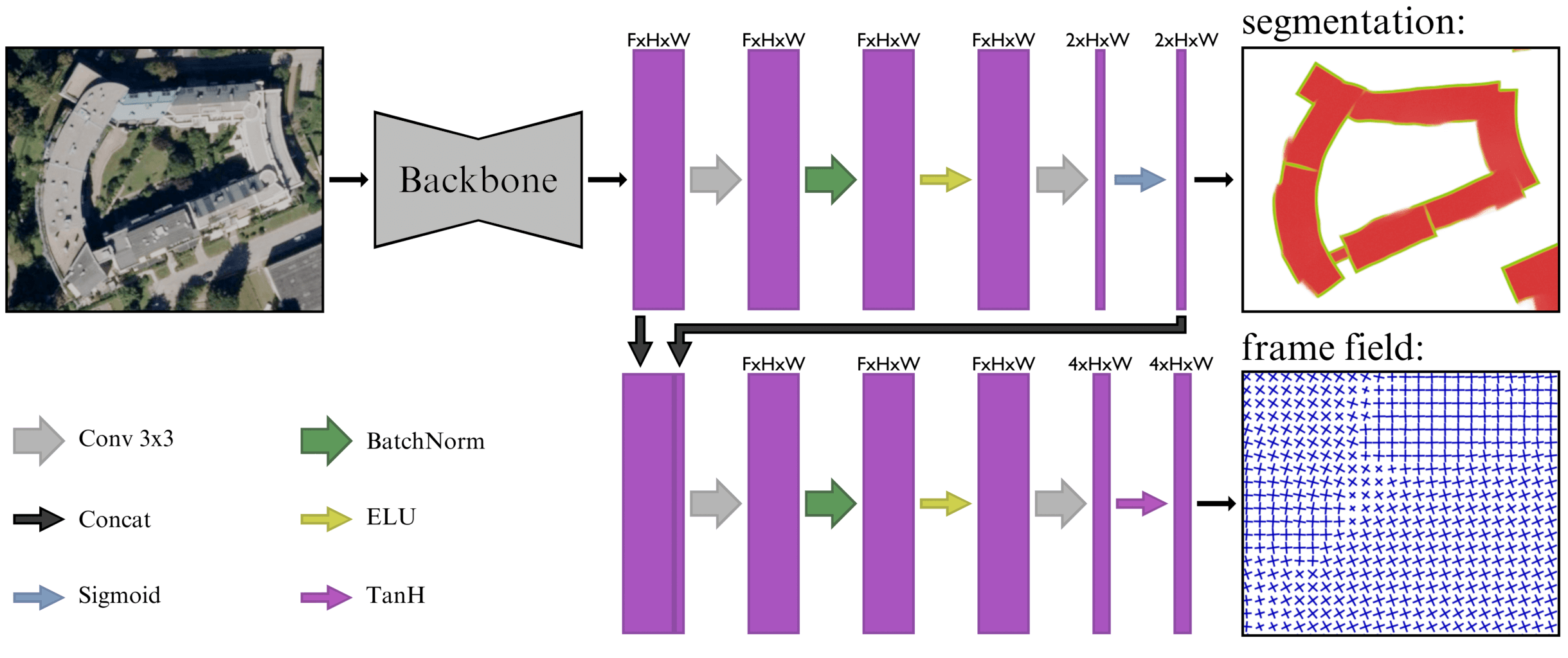
Figure S1: Details of our network’s architecture with the addition of the frame field output.

1.2 Losses

We define image segmentation loss functions below:

$$L_{\textit{BCE}}(y,\widehat{y})=\frac{1}{HW}\sum_{{x}\in I}y({x})\cdot\log(\widehat{y}({x}))\\ +(1-y({x}))\cdot\log(1-\widehat{y}({x})),$$ (9)

$$L_{\textit{Dice}}(y,\widehat{y})=1-2\cdot\frac{|y\cdot y|+1}{|y+y|+1},$$ (10)

$$L_{\textit{int}}=\alpha\cdot L_{\textit{BCE}}(y_{\textit{int}},\widehat{y}_{\textit{int}})+(1-\alpha)\cdot L_{\textit{Dice}}(y_{\textit{int}},\widehat{y}_{\textit{int}}),$$ (11)

$$L_{\textit{edge}}=\alpha\cdot L_{\textit{BCE}}(y_{\textit{edge}},\widehat{y}_{\textit{edge}})+(1-\alpha)\cdot L_{\textit{Dice}}(y_{\textit{edge}},\widehat{y}_{\textit{edge}}),$$ (12)

where $0<\alpha<1$ is a hyperparameter. In practice, $\alpha=0.25$ gives good results.

For the frame field, we show a visualization of the $L_{\textit{align}}$ loss in Fig. S2.

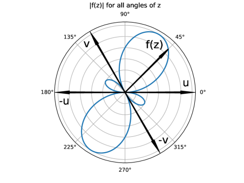
Figure S2: Visualization of the frame field align loss $L_{\textit{align}}$ (in blue) for a certain configuration of $\{-u,u,-v,v\}$ and all possible ground truth $z=e^{i\theta_{\tau}}$ directions.

1.3 Handling numerous heterogeneous losses

We linearly combine our eight losses using eight coefficients, which can be challenging to balance. Because the losses have different units, we first compute a normalization coefficient $N_{\langle\textit{loss name}\rangle}$ by computing the average of each loss on a random subset of the training dataset using a randomly-initialized network. Then each loss can be normalized by this coefficient. The total loss is a linear combination of all normalized losses:

$$\lambda_{\textit{int}}\frac{L_{\textit{int}}}{N_{\textit{int}}}+\lambda_{\textit{edge}}\frac{L_{\textit{edge}}}{N_{\textit{edge}}}+\lambda_{\textit{align}}\frac{L_{\textit{align}}}{N_{\textit{align}}}+\lambda_{\textit{align90}}\frac{L_{\textit{align90}}}{N_{\textit{align90}}}\\ +\lambda_{\textit{smooth}}\frac{L_{\textit{smooth}}}{N_{\textit{smooth}}}+\lambda_{\textit{int align}}\frac{L_{\textit{int align}}}{N_{\textit{int align}}}\\ +\lambda_{\textit{edge align}}\frac{L_{\textit{edge align}}}{N_{\textit{edge align}}}+\lambda_{\textit{int edge}}\frac{L_{\textit{int edge}}}{N_{\textit{int edge}}},$$ (13)

where the $\lambda_{\langle\textit{loss name}\rangle}$ coefficients are to be tuned. It is also possible to separately group the main losses and the regularization losses and have a single $\lambda$ coefficient balancing the two loss groups:

$$\lambda L_{\textit{main}}+(1-\lambda)L_{\textit{regularization}},$$ (14)

with

$$L_{\textit{main}}=\frac{L_{\textit{int}}}{N_{\textit{int}}}+\frac{L_{\textit{edge}}}{N_{\textit{edge}}}+\frac{L_{\textit{align}}}{N_{\textit{align}}},$$ (15)

$$L_{\textit{regularization}}=\frac{L_{\textit{align90}}}{N_{\textit{align90}}}+\frac{L_{\textit{smooth}}}{N_{\textit{smooth}}}\\ +\frac{L_{\textit{int align}}}{N_{\textit{int align}}}+\frac{L_{\textit{edge align}}}{N_{\textit{edge align}}}+\frac{L_{\textit{int edge}}}{N_{\textit{int edge}}}.$$ (16)

In practice we started experiments with the single-coefficient version with $\lambda=0.75$ and then used the multi-coefficient version to have more control by setting $\lambda_{\textit{int}}=\lambda_{\textit{edge}}=10$, $\lambda_{\textit{align}}=1$, $\lambda_{\textit{align90}}=0.2$, $\lambda_{\textit{smooth}}=0.005$, $\lambda_{\textit{int align}}=\lambda_{\textit{edge edge}}=\lambda_{\textit{int edge}}=0.2$.

1.4 Training details

We do not heavily tune our hyperparameters: once we find a value that works based on validation performance we keep it across ablation experiments. We employ early stopping for the U-Net16 and DeepLabV3 models (25 and 15 epochs, respectively) chosen by first training the full method on the training set of the CrowdAI dataset, choosing the epoch number of the lowest validation loss, and finally re-training the model on the train and validation sets for that number of total epochs.

Segmentation losses $L_{\textit{int}}$ and $L_{\textit{edge}}$ are both a combination of 25% cross-entropy loss and 75% Dice loss. To balance the losses in ablation experiments, we used the single-coefficient version with $\lambda=0.75$. For our best performing model UResNet101 we used the multi-coefficients version to have more control by setting $\lambda_{\textit{int}}=\lambda_{\textit{edge}}=10$, $\lambda_{\textit{align}}=1$, $\lambda_{\textit{align90}}=0.2$, $\lambda_{\textit{smooth}}=0.005$, $\lambda_{\textit{int align}}=\lambda_{\textit{edge edge}}=\lambda_{\textit{int edge}}=0.2$. The U-Net16 was trained on 4 GTX 1080Ti GPUs in parallel on $512\!\times\!512$ patches and a batch size of 16 per GPU (effective batch size 64). For all training runs, we compute for each loss its normalization coefficient $N_{\langle loss\_name\rangle}$ on 1000 batches before optimizing the network.

Our method is implemented in PyTorch [31]. On the CrowdAI dataset, training takes 2 hours per epoch on 4 1080Ti GPUs for the U-Net16 model and 3.5 hours per epoch for the DeepLabV3 backbone on 4 2080Ti GPUs. Inference with the U-Net16 on a $5000\!\times\!5000$ image (requires splitting into $1024\!\times\!1024$ patches) takes 7 seconds on a Quadro M2200 (laptop GPU).

2 Frame field polygonization details

We expand here on the algorithm and implementation details of our frame field polygonization method.

2.1 Data structure

Our polygonization method needs to be initialized with geometry, which is then optimized to align to the frame field (among other objectives we will present later).

In the case of extracting individual buildings, we use the marching squares [25] contour finding algorithm on the predicted interior probability map $y_{\textit{int}}$ with an isovalue $\ell$ (set to $0.5$ in practice). The result is a collection of contours $\{\mathcal{C}_{i}\}$ where each contour is a sequence of 2D points:

$$\mathcal{C}_{i}=\big{(}(r_{0},c_{0}),(r_{1},c_{1}),...,(r_{n_{i}-1},c_{n_{i}-1})\big{)}\,.$$

where $r_{i},c_{i}\in\mathbb{R}$ correspond to vertex $i$’s position along the row axis and the column axis respectively (they are not restricted to being integers). A contour is generally closed with $(r_{0},c_{0})=(r_{n_{i}-1},c_{n_{i}-1})$, but it can be open if the corresponding object touches the border of the image (therefore start and end vertices are not the same).

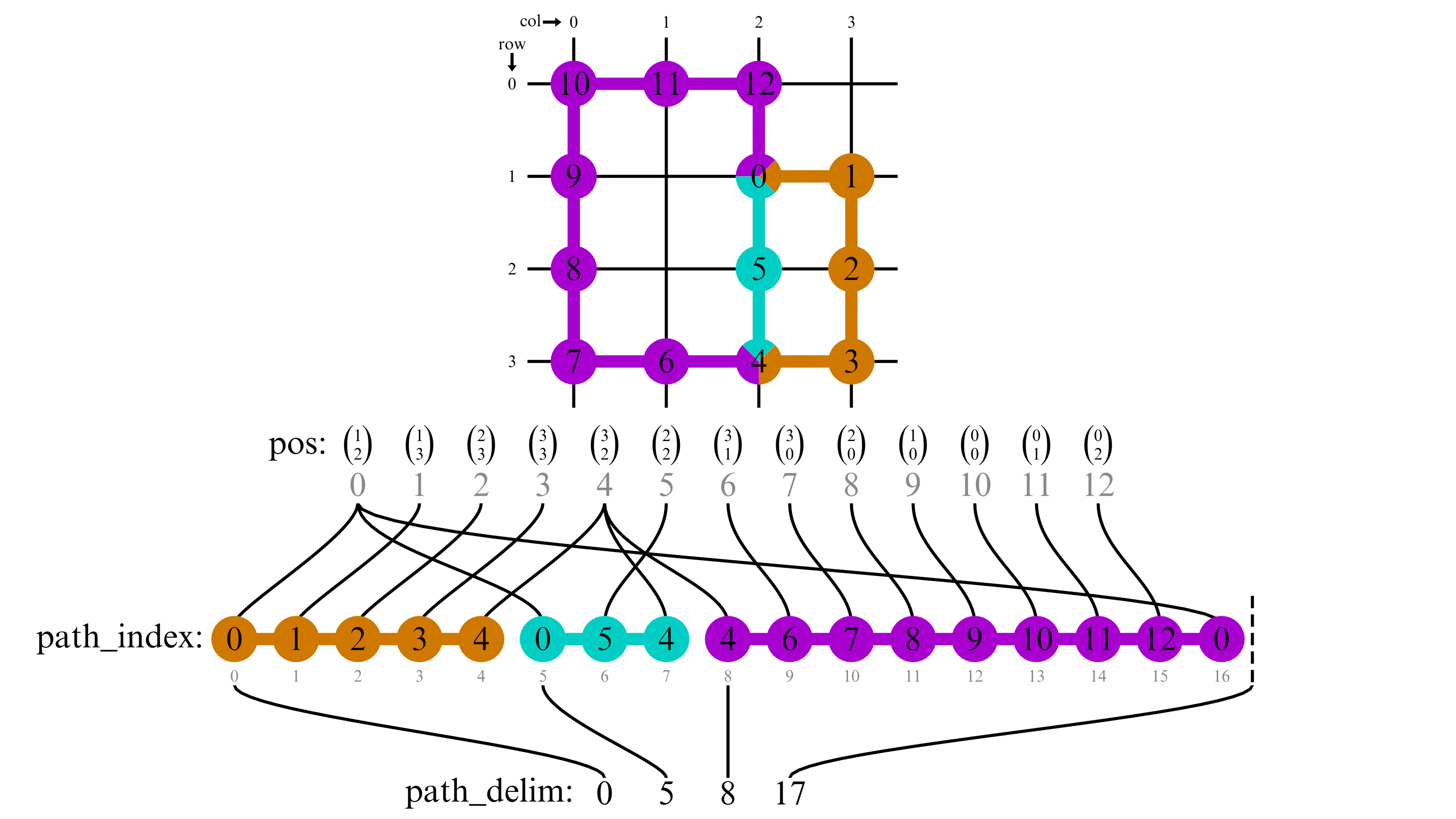
Figure S3: Our data structure of an example skeleton graph. It represents two buildings with a shared wall, necessitating 3 polyline paths. Here nodes $0$ and $4$ are shared among paths and are thus repeated in $path\_index$. We can see $path\_index$ is a concatenation of the node indices in $pos$ of the paths. Finally, $path\_delim$ is used to store the separation indices in $path\_index$ of those concatenated paths. Indices of arrays are in gray.

In the case of extracting buildings with potential adjoining buildings sharing a common wall, we extract the skeleton graph of the predicted edge probability map $y_{\textit{edge}}$. This skeleton graph is a hyper-graph made of nodes connected together by chains of vertices (i.e., polylines) called paths (see Fig. S4 for examples). To obtain this skeleton graph, we first compute the skeleton image using the thinning method [43] on the binary edge mask (computed by thresholding $y_{\textit{edge}}$ with $\ell=0.5$). It reduces binary objects to a one-pixel-wide representation. We then use the Skan [29] Python library to convert this representation to a graph representation connecting those pixels. The resulting graph is a collection of paths that are polylines connecting junction nodes together. We use an appropriate data structure only involving arrays (named tensors in deep learning frameworks) so that it can be manipulated by the GPU. We show in Fig. S3 an infographic of the data structure. A sequence of node coordinates “pos” holds the location of all nodes $i\in[0\mathinner{\ldotp\ldotp}n-1]$ belonging to the skeleton:

$$\textit{pos}=\big{(}(r_{0},c_{0}),(r_{1},c_{1}),...,(r_{n-1},c_{n-1})\big{)}\,$$

where $n$ is the total number of skeleton pixels and $(r_{i},c_{i})\in[0\mathinner{\ldotp\ldotp}H-1]\times[0\mathinner{\ldotp\ldotp}W-1]$ correspond to the row number and column number, respectively (of skeleton pixel $i$). The skeleton graph connects junction nodes through paths, which are polylines made up of connected vertices. These paths are represented by the “paths” binary matrix $P_{p,n}$ where element $(i,j)$ is one if node j is in path i. This $P_{p,n}$ is sparse, and, thus, it is more efficient to use the CSR (compressed sparse row) format, which represents a matrix by three (one-dimensional) arrays respectively containing nonzero values, the column indices and the extents of rows. As $P_{p,n}$ is binary we do not need the array containing non-zeros values. The column indices array, which we name “path_index” holds the column indices of all “on” elements:

$$\textit{path\_index}=(j_{0},j_{1},...,j_{n-n_{\textit{junctions}}+n_{\textit{degrees sum}}-1}),$$

where $n_{\textit{junctions}}$ is the total number of junction nodes, $n_{\textit{degrees sum}}$ is the sum of the degrees of all junction nodes and $\forall k\in[0\mathinner{\ldotp\ldotp}n-n_{\textit{junctions}}+n_{\textit{degrees sum}}-1],j_{k}\in[0\mathinner{\ldotp\ldotp}n-1]$. The extents of rows array which we name “$path\_delim$” holds the starting index of each row (it also contains an extra end element which is the number of non-zeros elements $n$ for easier computation):

$$\textit{path\_delim}=(s_{0},s_{1},...,s_{p})\,.$$

Thus, in order to get row $i$ of $P_{p,n}$ we need to look up the slice $(s_{i},s_{i+1})$ of $path\_index$. In the skeleton graph case, this representation is also easily interpretable. Indices of path nodes are all concatenated in path_index and path_delim is used to separate those concatenated paths. And finally a sequence of integers “degrees” stores for each node the number of nodes connected to it:

$$\textit{degrees}=(d_{0},d_{1},...,d_{n-1})\,.$$

As a collection of contours is a type of graph, in order to use a common data structure in our algorithm, we also use the skeleton graph representation for the contours $\{\mathcal{C}_{i}\}$ given by the marching squares algorithm (note we could use other contour detection algorithms for initialization). Each contour is thus an isolated path in the skeleton graph.

In order to fully leverage the parallelization capabilities of GPUs, the largest amount of data should be processed concurrently to increase throughput, i.e., we should aim to use the GPU memory at its maximum capacity. When processing a small image (such as $300\times 300$ pixels from the CrowdAI dataset), only a small fraction of memory is used. We thus build a batch of such small images to process them at the same time. As an example, on a GTX 1080Ti, we use a polygonization batch size $B=1024$ for processing the CrowdAI dataset, which induces a significant speedup. Building a batch of images is very simple: they can be concatenated together along an additional batch dimensions, i.e., $B$ images $I_{i}\in\mathbb{R}^{3\times H\times W}$ are grouped in a tensor $\mathbf{I}\in\mathbb{R}^{B\times 3\times H\times W}$. This is the case for the output segmentation probability maps as well as the frame field. However, it is slightly more complex to build a batch of skeleton graphs because of their varying sizes. Given a collection of skeleton graphs $\{(\textit{pos}_{i},\textit{degrees}_{i},\textit{path\_index}_{i},\textit{path\_delim}_{i})\}_{i\in[\mathinner{\ldotp\ldotp}B-1]}$, all $\textit{pos}_{i}$ and $\textit{degrees}_{i}$ are concatenated in their first dimension to give batch arrays:

$$\textit{pos}_{\textit{batch}}=[\textit{pos}_{0},\textit{pos}_{1},\ldots,\textit{pos}_{B-1}]\,,$$

and:

$$\textit{degrees}_{\textit{batch}}=[\textit{degrees}_{0},\textit{degrees}_{1},\ldots,\textit{degrees}_{B-1}].$$

All $\textit{path\_index}_{i}$ need their indices to be shifted by a certain offset:

$$\textit{offset}_{i}=\sum_{k=0}^{i-1}|\textit{pos}_{k}|,$$

with $|\textit{pos}_{k}|$ the number of points in $\textit{pos}_{k}$, so that they point to the new locations in $\textit{pos}_{\textit{batch}}$ and $\textit{degree}_{\textit{batch}}$. They are then concatenated in their first dimension: $\textit{path\_index}_{\textit{batch}}=[\textit{path\_index}_{0}+\textit{offset}_{0},\ldots,\textit{path\_index}_{B-1}+\textit{offset}_{B-1}].$ In a similar manner, we concatenate all $\textit{path\_delim}_{i}$ into $\textit{path\_delim}_{\textit{batch}}$ while taking care of adding the appropriate offset. We then obtain a big batch skeleton graph which is represented in the same way as a single skeleton graph. In order to later recover individual skeleton graphs in the batch, similar to path_delim, we need a batch_delim array that stores the starting index of each individual skeleton graph in the path_delim array (it also contains an extra end element which is the total number of paths in the batch for easier computation). While we apply the optimization on the batched arrays $pos_{batch}$, $path\_index_{batch}$, and so on, for readability we will now refer to them as $pos$, $path\_index$ and so on. Note that in the case of big images (such as $5000\times 5000$ pixels from the Inria dataset), we set the batch size to 1, as the probability maps, the frame field, and the skeleton graph data structure fills the GPU’s memory well.

At this point the data structure is fixed, i.e., it will not change during optimization. Only the values in $pos$ will be modified. This data structure is efficiently manipulated in parallel on the GPU. All the operations needed for the various computations performed in the next sections are run in parallel on the GPU.

We compute other tensors from this minimal data structure which will be useful for computations:

• path_pos = pos[path_index] which expands the positions tensor for each path (junction nodes are thus repeated in $path\_pos$).

• A $batch$ tensor which for each node in $pos\_batch$ stores the index $i\in[0\mathinner{\ldotp\ldotp}B-1]$ of the individual skeleton this node belongs to. This is used to easily sample the batched segmentation maps and the batched frame fields at the position of a node.

2.2 Active Skeleton Model

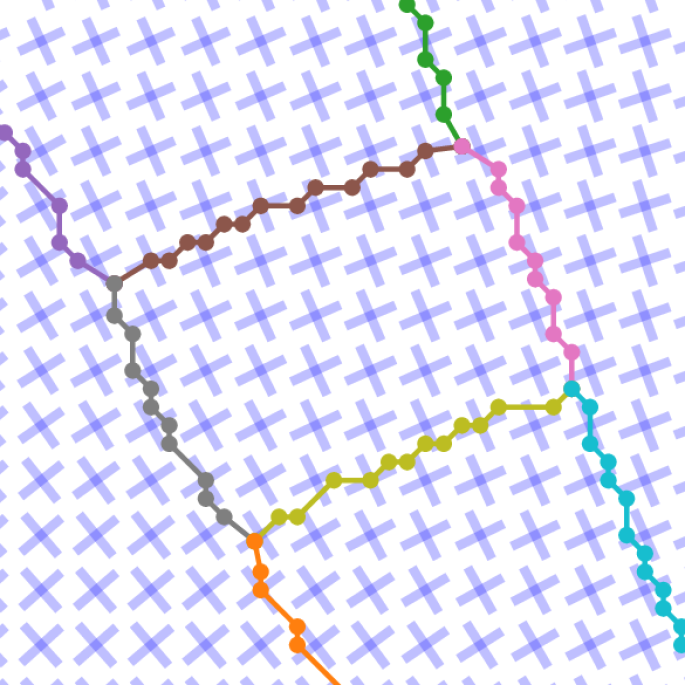
(a) Step 0

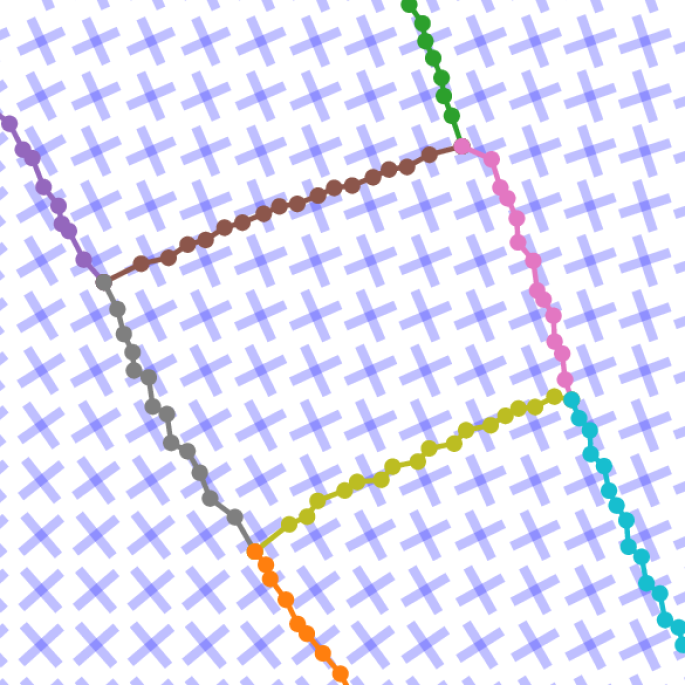
(b) Step 2

(c) Step 5

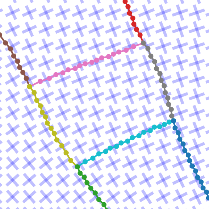
(d) Step 10

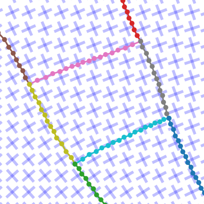
(e) Step 25

(f) Step 100

Figure S4: ASM optimization steps (zoomed example). Frame field in blue crosses.

We adapt the formulation of the Active Contours Model (ACM) to an Active Skeleton Model (ASM) in order to optimize our batch skeleton graph. The advantage of using the energy minimization formulation of ACM is to be able to add extra terms if needed (we can imagine adding regularization terms to, e.g., reward 90°corners, uniform curvature, and straight walls).

Energy terms will be parameterized by the node positions $\mathbf{p}\in pos$, which are the variables being optimized. The first important energy term is $E_{\textit{probability}}$ which aims to fit the skeleton paths to the contour of the building interior probability map $y_{\textit{int}}({v})$ at a certain probability level $\ell$ (which we set to 0.5 in practice, just like the isovalue used to initialize the contours by marching squares):

$$E_{\textit{probability}}=\sum_{\mathbf{p}\in pos}(y_{\textit{int}}(\mathbf{p})-l)^{2}\,.$$

The value $y_{\textit{int}}({\mathbf{p}})$ is computed by bilinear interpolation so that gradients can be back-propagated to $\mathbf{p}$. Additionally, $y_{\textit{int}}({\mathbf{p}})$ implicitly entails using the $batch$ array to know which slice in the batch dimension of $y_{\textit{int}}\in\mathbb{R}^{B\times 1\times H\times W}$ to sample $\mathbf{p}$ from. This will be the case anytime batched image-like tensors are sampled at a point $\mathbf{p}$. In the case of the marching squares initialization, this $E_{\textit{probability}}$ energy is actually zero at the start of optimization, since the initialized contour already is at isovalue $\ell$. For the skeleton graph initialization, paths that trace inner walls between adjoining buildings will not be affected since the gradient is zero in a neighborhood of homogeneous values (i.e., $y_{\textit{int}}=1$ inside buildings).

The second important energy term is $E_{\textit{frame field align}}$ which aligns each edge of the skeleton paths to the frame field. Edge vectors are computed in parallel as:

$${\mathbf{e}=\leavevmode\lstinline{{\lst@@@set@language\lst@@@set@numbers\lst@@@set@frame\lst@@@set@rulecolor{\@listingGroup{ltx_lst_identifier}{path\textunderscore pos}}[1:]{\@listingGroup{ltx_lst_space}{}}-{\@listingGroup{ltx_lst_space}{}}{\@listingGroup{ltx_lst_identifier}{path\textunderscore pos}}[:-1]}}}\,,$$

while taking care of removing from the energy computation “hallucinated” edges between paths (using the $path\_delim$ array). For readability we call $E$ the set of valid edge vectors. For each edge vector $\mathbf{e}\in E$, we refer to its direction as $\mathbf{e}_{dir}=\frac{\mathbf{e}}{\|\mathbf{e}\|}$. We also refer to its center point as ${\mathbf{e}_{\textit{center}}=\frac{1}{2}\leavevmode\lstinline{{\lst@@@set@language\lst@@@set@numbers\lst@@@set@frame\lst@@@set@rulecolor({\@listingGroup{ltx_lst_identifier}{path\textunderscore pos}}[1:]{\@listingGroup{ltx_lst_space}{}}+{\@listingGroup{ltx_lst_space}{}}{\@listingGroup{ltx_lst_identifier}{path\textunderscore pos}}[:-1])}}}$. The frame field align term is defined as:

$$E_{\textit{frame field align}}=\sum_{\mathbf{e}\in E}|f({\mathbf{e}_{\textit{dir}}};c_{0}({\mathbf{e}_{\textit{center}}}),c_{2}({\mathbf{e}_{\textit{center}}}))|^{2}\,.$$

This is the term that disambiguates between slanted walls and corners and results in regular-looking contours.

The last important term is the internal energy term $E_{\textit{length}}$ which ensures node distribution along paths remains homogeneous as well as tight:

$$E_{\textit{length}}=\sum_{\mathbf{e}\in E}|\mathbf{e}|^{2}\,.$$

All energy terms are then linearly combined: $E_{\textit{total}}=\lambda_{\textit{probability}}E_{\textit{probability}}+\lambda_{\textit{frame field align}}E_{\textit{frame field align}}+\lambda_{\textit{length}}E_{\textit{length}}\,.$ In practice, the final result is robust to different values of coefficients for each of these three energy terms, and we determine them using a small cross-validation set. The total energy is minimized with the RMSprop [40] gradient descent method with a smoothing constant $\gamma=0.9$ with an initial learning rate of $\eta=0.1$ which is exponentially decayed. The optimization is run for 300 iterations to ensure convergence. Indeed since the geometry is initialized to lie on building boundaries, it is not expected to move more than a few pixels and the optimization converges quickly. See Fig. S4 for a zoomed example of different stages of the ASM optimization.

2.3 Corner-aware polygon simplification

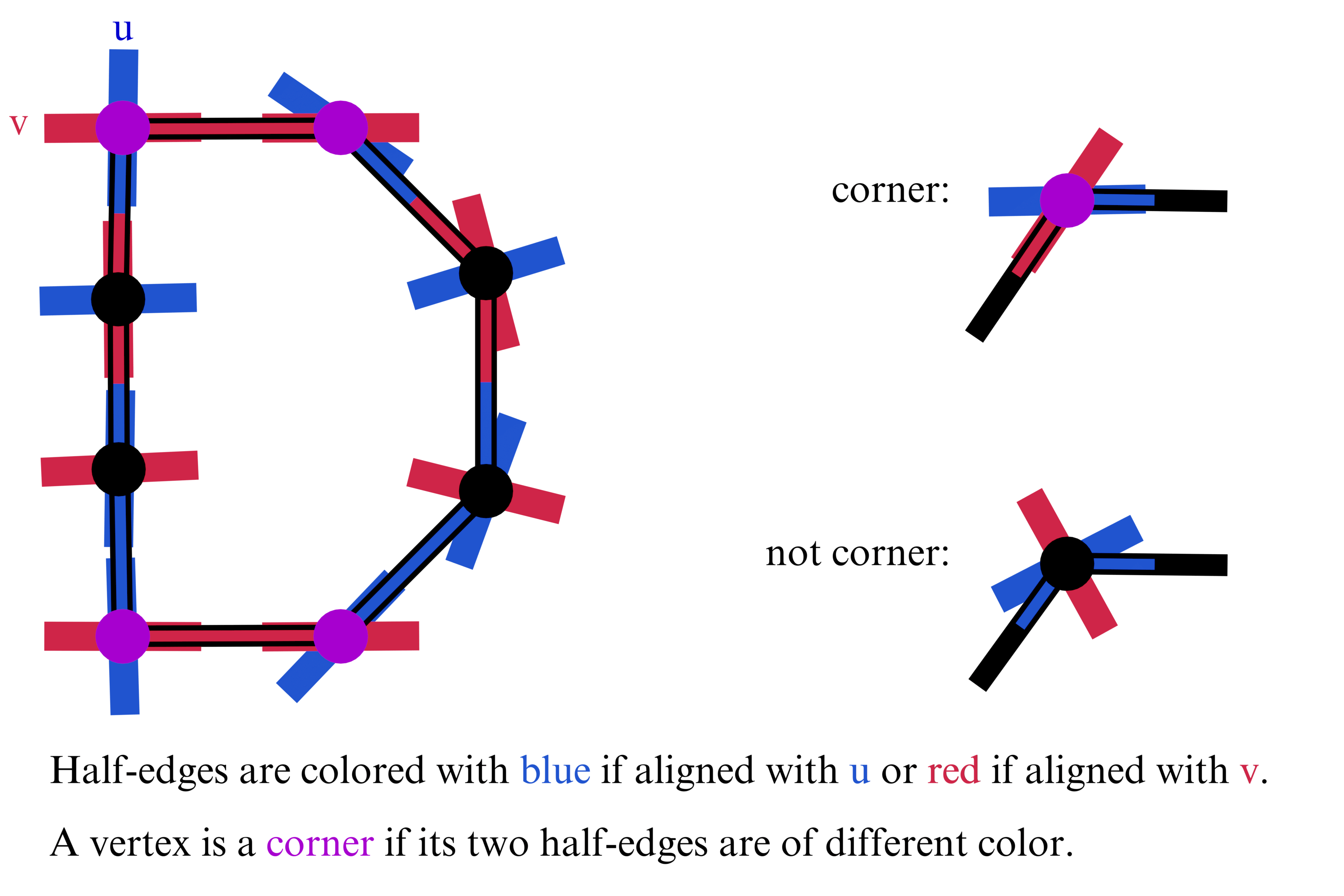
Figure S5: Corner detection using the frame field. For each vertex, the frame field is sampled at that location (with nearest neighbor) and represented by the $\{\pm{\color[rgb]{0,0,1}u},\pm{\color[rgb]{1,0,0}v}\}$ vectors.

We now have a collection of connected polylines that forms a planar skeleton graph. As building corners should not be removed during simplification, only polylines between corners are simplified. For the moment our data structure encodes a collection of polyline paths connecting junction nodes in the skeleton graph. However, a single path can represent multiple walls. It is the case for example of an individual rectangular building: one path describes its contour while it has 4 walls. In order to split paths into sub-paths each representing a single wall we need to detect building corners along a path and add this information to our data structure. This is another reason to use a frame field input, as it implicitly models corners: at a given building corner, there are two tangents of the contour. The frame field learned to align one of $u$ or $-u$ to the first tangent and one of $v$ or $-v$ to the other tangent. Thus when walking along a contour path if the local direction of walking switches from $\pm u$ to $\pm u$ or vice versa, it means we have come across a corner, see Fig. S5 for an infographic for corner detection. Specifically for each node $i$ with position ${\mathbf{p}=\leavevmode\lstinline{{\lst@@@set@language\lst@@@set@numbers\lst@@@set@frame\lst@@@set@rulecolor{\@listingGroup{ltx_lst_identifier}{path\textunderscore pos}}[{\@listingGroup{ltx_lst_identifier}{i}}]}}}$ its preceding and following edge vectors are computed as: ${\mathbf{e}_{\textit{prev}}=\leavevmode\lstinline{{\lst@@@set@language\lst@@@set@numbers\lst@@@set@frame\lst@@@set@rulecolor{\@listingGroup{ltx_lst_identifier}{path\textunderscore pos}}[{\@listingGroup{ltx_lst_identifier}{i}}]{\@listingGroup{ltx_lst_space}{}}-{\@listingGroup{ltx_lst_space}{}}{\@listingGroup{ltx_lst_identifier}{path\textunderscore pos}}[{\@listingGroup{ltx_lst_identifier}{i}}-1]}}}$ and $𝐞{}_{\text{next}}=\text{p}\text{a}\text{t}\text{h}\text{\_}\text{p}\text{o}\text{s}\text{[}\text{i}$

References

- [1] David Acuna, Huan Ling, Amlan Kar, and Sanja Fidler. Efficient interactive annotation of segmentation datasets with polygon-rnn++. In The IEEE Conference on Computer Vision and Pattern Recognition (CVPR), 2018.
- [2] Anil Batra, Suriya Singh, Guan Pang, Saikat Basu, C.V. Jawahar, and Manohar Paluri. Improved road connectivity by joint learning of orientation and segmentation. In The IEEE Conference on Computer Vision and Pattern Recognition (CVPR), June 2019.
- [3] Yoshua Bengio, Nicholas Léonard, and Aaron Courville. Estimating or propagating gradients through stochastic neurons for conditional computation. 2013. arXiv:1308.3432.
- [4] Mikhail Bessmeltsev and Justin Solomon. Vectorization of line drawings via polyvector fields. ACM Trans. Graph., 2019.
- [5] Lluıs Castrejón, Kaustav Kundu, Raquel Urtasun, and Sanja Fidler. Annotating object instances with a polygon-rnn. In The IEEE Conference on Computer Vision and Pattern Recognition (CVPR), 2017.
- [6] Bodhiswatta Chatterjee and Charalambos Poullis. On building classification from remote sensor imagery using deep neural networks and the relation between classification and reconstruction accuracy using border localization as proxy. In 2019 16th Conference on Computer and Robot Vision (CRV), pages 41–48, 2019.
- [7] Liang-Chieh Chen, George Papandreou, Florian Schroff, and Hartwig Adam. Rethinking atrous convolution for semantic image segmentation. 2017. arXiv:1706.05587.
- [8] Zhiqin Chen, Andrea Tagliasacchi, and Hao Zhang. Bsp-net: Generating compact meshes via binary space partitioning. Proceedings of IEEE Conference on Computer Vision and Pattern Recognition (CVPR), 2020.
- [9] Jakub Czakon, Kamil A. Kaczmarek, Andrzej Pyskir, and Piotr Tarasiewicz. Best practices for elegant experimentation in data science projects. EuroPython, 2018.
- [10] Jia Deng, Wei Dong, Richard Socher, Li-Jia Li, Kai Li, and Li Fei-Fei. ImageNet: A Large-Scale Hierarchical Image Database. In The IEEE Conference on Computer Vision and Pattern Recognition (CVPR), 2009.
- [11] Olga Diamanti, Amir Vaxman, Daniele Panozzo, and Olga Sorkine-Hornung. Designing -polyvector fields with complex polynomials. Eurographics SGP, 2014.
- [12] Lei Ding and Lorenzo Bruzzone. Diresnet: Direction-aware residual network for road extraction in vhr remote sensing images. 2020. arXiv:2005.07232.
- [13] David H. Douglas and Thomas K. Peucker. Algorithms for the reduction of the number of points required to represent a digitized line or its caricature. The Canadian Cartographer, 10(2):112–122, 1973.
- [14] Jun Gao, Zian Wang, Jinchen Xuan, and Sanja Fidler. Beyond fixed grid: Learning geometric image representation with a deformable grid. In ECCV, 2020.
- [15] Nicolas Girard, Guillaume Charpiat, and Yuliya Tarabalka. Noisy Supervision for Correcting Misaligned Cadaster Maps Without Perfect Ground Truth Data. In IEEE International Geoscience and Remote Sensing Symposium (IGARSS), 2019.
- [16] Kaiming He, Georgia Gkioxari, Piotr Dollar, and Ross Girshick. Mask r-cnn. In The IEEE International Conference on Computer Vision (ICCV), Oct 2017.
- [17] Kaiming He, Xiangyu Zhang, Shaoqing Ren, and Jian Sun. Deep residual learning for image recognition. 2015. arXiv:1512.03385.
- [18] Sepp Hochreiter and Jürgen Schmidhuber. Long short-term memory. Neural computation, 9:1735–80, 12 1997.
- [19] Michael Kass, Andrew Witkin, and Demetri Terzopoulos. Snakes: Active contour models. International Journal of Computer Vision (IJCV), 1(4):321–331, 1988.
- [20] Muxingzi Li, Florent Lafarge, and Renaud Marlet. Approximating shapes in images with low-complexity polygons. In The IEEE Conference on Computer Vision and Pattern Recognition (CVPR), 2020.
- [21] Zuoyue Li, Jan Dirk Wegner, and Aurélien Lucchi. Topological map extraction from overhead images. In The IEEE International Conference on Computer Vision (ICCV), 2019.
- [22] Tsung-Yi Lin, Michael Maire, Serge Belongie, James Hays, Pietro Perona, Deva Ramanan, Piotr Dollár, and C. Lawrence Zitnick. Microsoft coco: Common objects in context. In David Fleet, Tomas Pajdla, Bernt Schiele, and Tinne Tuytelaars, editors, The European Conference on Computer Vision (ECCV), pages 740–755, Cham, 2014. Springer International Publishing.
- [23] Huan Ling, Jun Gao, Amlan Kar, Wenzheng Chen, and Sanja Fidler. Fast interactive object annotation with curve-gcn. In The IEEE Conference on Computer Vision and Pattern Recognition (CVPR), 2019.
- [24] Shu Liu, Lu Qi, Haifang Qin, Jianping Shi, and Jiaya Jia. Path aggregation network for instance segmentation. In Proceedings of IEEE Conference on Computer Vision and Pattern Recognition (CVPR), 2018.
- [25] William Lorensen and Harvey E. Cline. Marching cubes: A high resolution 3d surface construction algorithm. 1987.
- [26] Emmanuel Maggiori, Yuliya Tarabalka, Guillaume Charpiat, and Pierre Alliez. Can semantic labeling methods generalize to any city? the inria aerial image labeling benchmark. In IEEE International Geoscience and Remote Sensing Symposium (IGARSS), 2017.
- [27] Volodymyr Mnih, Koray Kavukcuoglu, David Silver, Alex Graves, Ioannis Antonoglou, Daan Wierstra, and Martin A. Riedmiller. Playing atari with deep reinforcement learning. 2013. arXiv:1312.5602.
- [28] Volodymyr Mnih, Koray Kavukcuoglu, David Silver, Andrei A. Rusu, Joel Veness, Marc G. Bellemare, Alex Graves, Martin Riedmiller, Andreas K. Fidjeland, Georg Ostrovski, Stig Petersen, Charles Beattie, Amir Sadik, Ioannis Antonoglou, Helen King, Dharshan Kumaran, Daan Wierstra, Shane Legg, and Demis Hassabis. Human-level control through deep reinforcement learning. Nature, 518(7540):529–533, Feb. 2015.
- [29] Juan Nunez-Iglesias. skan: skeleton analysis in python. https://github.com/jni/skan, 2017.
- [30] OpenStreetMap contributors. Planet dump retrieved from https://planet.osm.org , 2017.
- [31] Adam Paszke, Sam Gross, Francisco Massa, Adam Lerer, James Bradbury, Gregory Chanan, Trevor Killeen, Zeming Lin, Natalia Gimelshein, Luca Antiga, Alban Desmaison, Andreas Kopf, Edward Yang, Zachary DeVito, Martin Raison, Alykhan Tejani, Sasank Chilamkurthy, Benoit Steiner, Lu Fang, Junjie Bai, and Soumith Chintala. Pytorch: An imperative style, high-performance deep learning library. In Advances in Neural Information Processing Systems 32, pages 8024–8035. Curran Associates, Inc., 2019.
- [32] Urs Ramer. An iterative procedure for the polygonal approximation of plane curves. Computer graphics and image processing, 1(3):244–256, 1972.
- [33] Olaf Ronneberger, Philipp Fischer, and Thomas Brox. U-net: Convolutional networks for biomedical image segmentation. 2015. arXiv:1505.04597.
- [34] Sharada Prasanna Mohanty. Crowdai dataset. https://www.crowdai.org/challenges/mapping-challenge/dataset_files, 2018.
- [35] Sharada Prasanna Mohanty. Crowdai mapping challenge 2018: Baseline with mask rcnn. https://github.com/crowdai/crowdai-mapping-challenge-mask-rcnn, 2018.
- [36] Carole H Sudre, Wenqi Li, Tom Vercauteren, Sebastien Ourselin, and M Jorge Cardoso. Generalised dice overlap as a deep learning loss function for highly unbalanced segmentations. In Deep learning in medical image analysis and multimodal learning for clinical decision support, pages 240–248. Springer, 2017.
- [37] Richard S. Sutton and Andrew G. Barto. Reinforcement learning: An introduction, 2020.
- [38] Maria Taktasheva, Albert Matveev, Alexey Artemov, and Evgeny Burnaev. Learning to approximate directional fields defined over 2d planes. In Wil M. P. van der Aalst, Vladimir Batagelj, Dmitry I. Ignatov, Michael Khachay, Valentina Kuskova, Andrey Kutuzov, Sergei O. Kuznetsov, Irina A. Lomazova, Natalia Loukachevitch, Amedeo Napoli, Panos M. Pardalos, Marcello Pelillo, Andrey V. Savchenko, and Elena Tutubalina, editors, Analysis of Images, Social Networks and Texts, pages 367–374, Cham, 2019. Springer International Publishing.
- [39] Meng Tang, Federico Perazzi, Abdelaziz Djelouah, Ismail Ben Ayed, Christopher Schroers, and Yuri Boykov. On regularized losses for weakly-supervised cnn segmentation. In The European Conference on Computer Vision (ECCV), 2018.
- [40] T. Tieleman and G. Hinton. Lecture 6.5—RmsProp: Divide the gradient by a running average of its recent magnitude. COURSERA: Neural Networks for Machine Learning, 2012.
- [41] S. Tripodi, L. Duan, F. Trastour, V. Poujad, Lionel Laurore, and Yuliya Tarabalka. Automated chain for large-scale 3d reconstruction of urban scenes from satellite images. ISPRS - International Archives of the Photogrammetry, Remote Sensing and Spatial Information Sciences, XLII-2/W16:243–250, 09 2019.
- [42] Amir Vaxman, Marcel Campen, Olga Diamanti, Daniele Panozzo, David Bommes, Klaus Hildebrandt, and Mirela Ben-Chen. Directional field synthesis, design and processing. Computer Graphics Forum, 35:545–572, 05 2016.
- [43] T. Y. Zhang and C. Y. Suen. A fast parallel algorithm for thinning digital patterns. Commun. ACM, 27(3):236–239, Mar. 1984.
- [44] Stefano Zorzi, Ksenia Bittner, and Friedrich Fraundorfer. Machine-learned regularization and polygonization of building segmentation masks, 2020. arXiv:2007.12587.
- [45] Stefano Zorzi and Friedrich Fraundorfer. Regularization of building boundaries in satellite images using adversarial and regularized losses. In IEEE International Geoscience and Remote Sensing Symposium (IGARSS), 2019.