Energy Conservation in the thin layer approximation: I. The spherical classic case for supernovae remnants

Abstract

The thin layer approximation applied to the expansion of a supernova remnant assumes that all the swept mass resides in a thin shell. The law of motion in the thin layer approximation is therefore found using the conservation of momentum. Here we instead introduce the conservation of energy in the framework of the thin layer approximation. The first case to be analysed is that of an interstellar medium with constant density and the second case is that of 7 profiles of decreasing density with respect to the centre of the explosion. The analytical and numerical results are applied to 4 supernova remnants: Tycho, Cas A, Cygnus loop, and SN 1006. The back reaction due to the radiative losses for the law of motion is evaluated in the case of constant density of the interstellar medium.

Keywords: supernovae: general, supernovae: individual (SN Tycho), supernovae: individual (SN Cas A), supernovae: individual (SN Cygnus loop), supernovae: individual (SN 1006)

1 Introduction

The thin layer approximation assumes that the mass ejected in the explosion of a supernova (SN) resides in a thin layer. This approximation is usually applied in the late stage of the explosion in order to explain the supernova remnant (SNR), see [1, 2, 3]. The physical quantity which is conserved in the previous approaches is the momentum, equal to the swept mass multiplied by the velocity at a given radius of expansion $r_{0}$ equated to these quantities at a radius $r$. Some natural questions therefore arise:

• Can we model the expansion of an SNR when the energy is conserved rather than the momentum?

• Can we model the energy conservation when the density of the interstellar medium (ISM) decreases with the distance from the point of the explosion?

In order to answer the above questions, Section; 2 reviews the standard laws of conservation, Section 3 introduces the conservation of energy and Section 4 applies the derived equations of motion to 4 SNRs.

2 Laws of conservation

We summarise four laws of conservation useful to model some astrophysical phenomena in which the temperature and the pressure are absent. The first law is the conservation of momentum in spherical coordinates in the framework of the thin layer approximation. The Newton’s second law for an expanding sphere in the framework of the thin shell approximation along a solid angle $\Delta\Omega$ is

$$\frac{d}{dt}\bigl{(}\frac{1}{3}r^{3}\rho v\big{)}=r^{2}P\quad,$$ (1)

where $r$ is the advancing radius, $\rho$ is the density assumed to be constant, $v$ the velocity and $P$ the internal pressure, see formula (10.27) in [4]. Let us assume $P=0$ (cold model) and the above equation in two different points of expansion becomes

$$M_{0}(r_{0})\,v_{0}=M(r)\,v\quad,$$ (2)

where $M_{0}(r_{0})$ and $M(r)$ are the swept masses at $r_{0}$ and $r$, while $v_{0}$ and $v$ are the velocities of the thin layer at $r_{0}$ and $r$. This first law has been widely used to model the SNRs, see [5, 6, 7, 8, 9, 10]. This conservation law can be expressed as a differential equation of the first order by inserting $v=\frac{dr}{dt}$:

$$M_{0}(r_{0})\,v_{0}=M(r)\,\frac{dr}{dt}\quad.$$ (3)

In the case where the ISM has constant density, the analytical solution for the trajectory is

$$r(t;t_{0},r_{0},v_{0})=\sqrt[4]{4\,{r_{{0}}}^{3}v_{{0}}\left(t-t_{{0}}\right)+{r_{{0}}}^{4}}\quad,$$ (4)

and the velocity is

$$v(t;t_{0},r_{0},v_{0})=\frac{{r_{{0}}}^{3}v_{{0}}}{\left(4\,{r_{{0}}}^{3}v_{{0}}\left(t-t_{{0}}\right)+{r_{{0}}}^{4}\right)^{3/4}}\quad,$$ (5)

where $r_{0}$ and $v_{0}$ are the position and the velocity when $t=t_{0}$. The second law is the conservation of energy which will be introduced in details in the next section. An example is given by the energy conserving phase in the interstellar bubbles, see [4]. The third law of conservation is given by the conservation of momentum flux which is the rate of transfer of momentum through a unit area

$$\rho(x_{0})v_{0}^{2}A(x_{0})=\rho(x)v(x)^{2}A(x)\quad,$$ (6)

where $\rho(x)$ is the density at position $x$, $A(x)$ is the area at position $x$ and $v(x)$ is the velocity at position $x$, see Formula A27 in [11]. This law is useful to model the radiogalaxies where there is a continuous flow of matter from the central region to the periphery, see [12]. The fourth law of conservation is given by the conservation of energy flux which is the rate of transfer of energy through a unit area

$$\frac{1}{2}\rho(x_{0})v_{0}^{3}A(x_{0})=\frac{1}{2}\rho(x)v(x)^{3}A(x)$$ (7)

where $\rho(x)$ is the density at position $x$, $A(x)$ is the area at position $x$ and $v(x)$ is the velocity at position $x$, see Formula A28 in [11]. This law is useful to model the astrophysical jets, see [13]

3 Energy conservation

The conservation of kinetic energy in spherical coordinates within the framework of the thin layer approximation when the thermal effects are negligible is

$$\frac{1}{2}M_{0}(r_{0})\,v_{0}^{2}=\frac{1}{2}M(r)\,v^{2}\quad,$$ (8)

where $M_{0}(r_{0})$ and $M(r)$ are the swept masses at $r_{0}$ and $r$, while $v_{0}$ and $v$ are the velocities of the thin layer at $r_{0}$ and $r$. The above conservation law, when written as a differential equation, is

$$\frac{1}{2}\,M\left(r\right)\left({\frac{\rm d}{{\rm d}t}}r\left(t\right)\right)^{2}-\frac{1}{2}\,{\it M_{0}}\,{{\it v_{0}}}^{2}=0\quad.$$ (9)

The velocity as a function of the momentary radius is

$$v(r;r_{0},v_{0})={\frac{{r_{{0}}}^{3/2}v_{{0}}}{{r}^{3/2}}}\quad.$$ (10)

In the following, the case of constant density as well as 7 profiles of decreasing density will be considered.

3.1 Medium with constant density

When the ISM is considered to have constant density, the analytical solution for the trajectory when the energy is conserved is

$$r(t;t_{0},r_{0},v_{0})=\frac{1}{2}\,{2}^{3/5}{r_{{0}}}^{3/5}\left(\left(5\,t-5\,t_{{0}}\right)v_{{0}}+2\,r_{{0}}\right)^{2/5}\quad,$$ (11)

which has the asymptotic behaviour $r_{a}(t;t_{0},r_{0},v_{0})$,

$$r_{a}(t;t_{0},r_{0},v_{0})\sim\frac{1}{2}\,{\frac{{2}^{3/5}{r_{{0}}}^{3/5}{5}^{2/5}{v_{{0}}}^{2/5}}{\left({t}^{-1}\right)^{2/5}}}+\frac{1}{25}\,{\frac{{2}^{3/5}{r_{{0}}}^{3/5}{5}^{2/5}\left(-5\,t_{{0}}v_{{0}}+2\,r_{{0}}\right)\left({t}^{-1}\right)^{3/5}}{{v_{{0}}}^{3/5}}}\quad.$$ (12)

The velocity as function of the radius is

$$v(r;r_{0},v_{0})={\frac{{r_{{0}}}^{3/2}v_{{0}}}{{r}^{3/2}}}\quad,$$ (13)

and the velocity as a function of time is

$$v(t;t_{0},r_{0},v_{0})={\frac{{2}^{3/5}{r_{{0}}}^{3/5}v_{{0}}}{\left(\left(5\,t-5\,t_{{0}}\right)v_{{0}}+2\,r_{{0}}\right)^{3/5}}}\quad,$$ (14)

where $r_{0}$ and $v_{0}$ are the position and the velocity when $t=t_{0}$.

3.2 Constant density and back reaction

The radiative losses per unit length are assumed to be proportional to the flux of momentum

$$-\epsilon\rho_{s}v^{2}4\,\pi r^{2}\quad,$$ (15)

where $\epsilon$ is a constant and $rho_{s}$ is density in the thin advancing layer which is $4\,\rho$. Inserting in the above equation the velocity to first order as given by equation (13) the radiative losses, $Q(r;r_{0},v_{0},\epsilon)$, are

$$Q(r;r_{0},v_{0},\epsilon)=-16\,{\frac{\epsilon\,\rho\,{r_{{0}}}^{3}{v_{{0}}}^{2}\pi}{r}}\quad.$$ (16)

The sum of the radiative losses between $r_{0}$ and $r$ is given by the following integral, $L$,

$$L(r;r_{0},v_{0},\epsilon)=\int_{r_{0}}^{r}Q(r;r_{0},v_{0},\epsilon)dr=-16\,\epsilon\,\rho\,{r_{{0}}}^{3}{v_{{0}}}^{2}\pi\,\ln\left(r\right)+16\,\epsilon\,\rho\,{r_{{0}}}^{3}{v_{{0}}}^{2}\pi\,\ln\left(r_{{0}}\right)\quad.$$ (17)

The conservation of energy in presence of the back reaction due to the radiative losses is

$$2/3\,\rho\,\pi\,{r}^{3}{v}^{2}+16\,\epsilon\,\rho\,{r_{{0}}}^{3}{v_{{0}}}^{2}\pi\,\ln\left(r\right)-16\,\epsilon\,\rho\,{r_{{0}}}^{3}{v_{{0}}}^{2}\pi\,\ln\left(r_{{0}}\right)=2/3\,\rho\,\pi\,{r_{{0}}}^{3}{v_{{0}}}^{2}\quad.$$ (18)

The analytical solution for the velocity to second order, $v_{c}(r;r_{0},c_{0},\epsilon)$, is

$$v_{c}(r;r_{0},v_{0},\epsilon)={\frac{{r_{{0}}}^{3/2}\sqrt{-24\,\ln\left(r\right)\epsilon+24\,\ln\left(r_{{0}}\right)\epsilon+1}v_{{0}}}{{r}^{3/2}}}\quad.$$ (19)

The inclusion of back reaction allows the evaluation of the SRS’s maximum length $r_{back}(r_{0},\epsilon)$ , which can be derived imposing to zero the above velocity.

$$r_{back}(r_{0},\epsilon)={{\rm e}^{1/24\,{\frac{24\,\ln\left(r_{{0}}\right)\epsilon+1}{\epsilon}}}}\quad.$$ (20)

3.3 Medium with an hyperbolic profile of density

We assume that the medium around the SN scales with the piecewise dependence

$$\rho(r;r_{0})=\{\begin{array}[]{ll}\rho_{c}&\mbox{if $r\leq r_{0}$ }\\ \rho_{c}(\frac{r_{0}}{r})&\mbox{if $r>r_{0}$.}\end{array},$$ (21)

where $\rho_{c}$ is the density at $r=0$ and $r_{0}$ is the radius after which the density starts to decrease. The mass swept, $M_{0}$, in the interval [0,$r_{0}$] is

$$M_{0}(\rho_{c},r_{0})=\frac{4}{3}\,\rho_{{c}}\pi\,{r_{{0}}}^{3}\quad.$$

The total mass swept, $M(r;r_{0},\rho_{c})$, in the interval [0,r] is

$$M(r;r_{0},\rho_{c})=-\frac{2}{3}\,\rho_{{c}}\pi\,{r_{{0}}}^{3}+2\,\rho_{{c}}r_{{0}}{r}^{2}\pi\quad.$$

The application of energy conservation gives the velocity as a function of the radius:

$$v(r;r_{0},v_{0})=2\,{\frac{v_{{0}}r_{{0}}}{\sqrt{6\,{r}^{2}-2\,{r_{{0}}}^{2}}}}\quad.$$ (22)

Separation of variables followed by integration gives

$$\frac{1}{12}\,{\frac{r_{{0}}\sqrt{6}\ln\left(\sqrt{2}+\sqrt{3}\right)}{v_{{0}}}}-\frac{1}{12}\,{\frac{r_{{0}}\sqrt{6}\ln\left(r\sqrt{2}\sqrt{3}+\sqrt{6\,{r}^{2}-2\,{r_{{0}}}^{2}}\right)}{v_{{0}}}}+\frac{1}{24}\,{\frac{r_{{0}}\sqrt{6}\ln\left(2\right)}{v_{{0}}}}$$

$$+\frac{1}{12}\,{\frac{r_{{0}}\sqrt{6}\ln\left(r_{{0}}\right)}{v_{{0}}}}+\frac{1}{4}\,{\frac{r\sqrt{6\,{r}^{2}-2\,{r_{{0}}}^{2}}}{v_{{0}}r_{{0}}}}-\frac{1}{2}\,{\frac{r_{{0}}}{v_{{0}}}}=t-t0\quad.$$ (23)

In this equation it is not possible to extract the radius as a function of time, and therefore a numerical procedure is adopted in order to derive the trajectory.

3.4 Medium with an inverse square profile for the density

We now assume that the medium around the SN scales with the piecewise dependence (which avoids a pole at $r=0$)

$$\rho(r;r_{0})=\{\begin{array}[]{ll}\rho_{c}&\mbox{if $r\leq r_{0}$ }\\ \rho_{c}(\frac{r_{0}}{r})^{2}&\mbox{if $r>r_{0}$.}\end{array},$$ (24)

where $\rho_{c}$ is the density at $r=0$ and $r_{0}$ is the radius after which the density starts to decrease.

The total mass swept, $M(r;r_{0},\rho_{c})$, in the interval [0,r] is

$$M(r;r_{0},\rho_{c})=-\frac{8}{3}\,\rho_{{c}}\pi\,{r_{{0}}}^{3}+4\,\rho_{{c}}{r_{{0}}}^{2}\pi\,r+\frac{4}{3}\,\rho_{{c}}\pi\,{r_{{0}}}^{3}\quad.$$

Applying the conservation of energy, the velocity as a function of the radius is

$$v(r;r_{0},v_{0})=-{\frac{\sqrt{-\left(2\,r_{{0}}-3\,r\right)r_{{0}}}v_{{0}}}{2\,r_{{0}}-3\,r}}\quad.$$ (25)

The trajectory, i.e. the radius as a function of time, is

$$r(t;t_{0},r_{0},v_{0})=\frac{1}{6}\,\sqrt[3]{2}\sqrt[3]{r_{{0}}}\left(\left(9\,t-9\,t_{{0}}\right)v_{{0}}+2\,r_{{0}}\right)^{2/3}+\frac{2}{3}\,r_{{0}}\quad,$$ (26)

which has the asymptotic behavior, $r_{a}(t;t_{0},r_{0},v_{0})$,

$$r_{a}(t;t_{0},r_{0},v_{0})\sim\frac{1}{6}\,{\frac{\sqrt[3]{2}\sqrt[3]{r_{{0}}}{9}^{2/3}{v_{{0}}}^{2/3}}{\left({t}^{-1}\right)^{2/3}}}+\frac{2}{3}\,r_{{0}}+{\frac{\sqrt[3]{2}\sqrt[3]{r_{{0}}}{9}^{2/3}\left(-9\,t_{{0}}v_{{0}}+2\,r_{{0}}\right)\sqrt[3]{{t}^{-1}}}{81\,\sqrt[3]{v_{{0}}}}}\quad.$$ (27)

The velocity as a function of time is

$$v(t;t_{0},r_{0},v_{0})={\frac{\sqrt[3]{2}\sqrt[3]{r_{{0}}}v_{{0}}}{\sqrt[3]{\left(9\,t-9\,t_{{0}}\right)v_{{0}}+2\,r_{{0}}}}}\quad.$$ (28)

3.5 Medium with a power law profile for the density

We now assume that the medium around the SN scales as

$$\rho(r;r_{0})=\{\begin{array}[]{ll}\rho_{c}&\mbox{if $r\leq r_{0}$ }\\ \rho_{c}(\frac{r_{0}}{r})^{\alpha}&\mbox{if $r>r_{0}$.}\end{array},$$ (29)

where $\rho_{c}$ is the density at $r=0$, $r_{0}$ is the radius after which the density starts to decrease and $\alpha>0$.

The total mass swept, $M(r;r_{0},\rho_{c},\alpha)$, in the interval [0,r] is

$$M(r;r_{0},\rho_{c},\alpha)=\frac{4}{3}\,\rho_{{c}}\pi\,{r_{{0}}}^{3}-4\,{\frac{{r}^{3}\rho_{{c}}\pi}{\alpha-3}\left({\frac{r_{{0}}}{r}}\right)^{\alpha}}+4\,{\frac{\rho_{{c}}\pi\,{r_{{0}}}^{3}}{\alpha-3}}\quad.$$

The application of energy conservation gives the differential equation

$$\frac{1}{3\,\alpha-9}\Bigg{(}-2\,\rho_{{c}}\pi\,\left(3\,{r}^{3}\left({\frac{r_{{0}}}{r}}\right)^{\alpha}-{r_{{0}}}^{3}\alpha\right)\left({\frac{\rm d}{{\rm d}t}}r\left(t\right)\right)^{2}\Bigg{)}=\frac{2}{3}\,\rho_{{c}}\pi\,{r_{{0}}}^{3}{v_{{0}}}^{2}\quad.$$ (30)

The velocity as a function of the radius is

$$v(r;r_{0},v_{0},\alpha)={\frac{\sqrt{-\left(-{r_{{0}}}^{3}\alpha+3\,{r}^{3-\alpha}{r_{{0}}}^{\alpha}\right)r_{{0}}\left(\alpha-3\right)}v_{{0}}r_{{0}}}{-{r_{{0}}}^{3}\alpha+3\,{r}^{3-\alpha}{r_{{0}}}^{\alpha}}}\quad.$$ (31)

There is no analytical solution for the trajectory, and therefore we have implemented a numerical procedure. The first approximation for the trajectory is obtained by a series solution of Equation (30) to fourth order,

$$r(t;r_{0},v_{0},t_{0},\alpha)\approx r_{{0}}+v_{{0}}\left(t-t_{{0}}\right)-\frac{3}{4}\,{\frac{{v_{{0}}}^{2}\left(t-t_{{0}}\right)^{2}}{r_{{0}}}}+\frac{1}{4}\,{\frac{{v_{{0}}}^{3}\left(\alpha+4\right)\left(t-t_{{0}}\right)^{3}}{{r_{{0}}}^{2}}}\quad.$$ (32)

The second approximation for the trajectory is found by first deriving an asymptotic expansion of Equation (31), namely

$$v(r;r_{0},v_{0},\alpha)\sim\frac{1}{3}\,{\frac{v_{{0}}r_{{0}}\sqrt{3}\sqrt{{r_{{0}}}^{\alpha+1}\left(3-\alpha\right)}}{{r_{{0}}}^{\alpha}\sqrt{\left({r}^{-1}\right)^{\alpha-3}}}}\quad.$$ (33)

Then, the asymptotic approximate trajectory turns out to be

$$r(t;r_{0},v_{0},t_{0},\alpha)\sim{12}^{\left(\alpha-5\right)^{-1}}{r_{{0}}}^{{\frac{\alpha-3}{\alpha-5}}}\times$$

$$\left(-4\,r_{{0}}v_{{0}}\left(\alpha-5\right)\left(t-t_{{0}}\right)\sqrt{9-3\,\alpha}-\left(\alpha-3\right)\left(\alpha-5\right)^{2}\left(t-t_{{0}}\right)^{2}{v_{{0}}}^{2}+12\,{r_{{0}}}^{2}\right)^{-\left(\alpha-5\right)^{-1}}\quad.$$ (34)

3.6 Medium with an exponential profile for the density

We assume that the medium around the SN scales with the piecewise dependence

$$\rho(r;r_{0})=\{\begin{array}[]{ll}\rho_{c}&\mbox{if $r\leq r_{0}$ }\\ \rho_{c}(\exp{-\frac{r}{b}})&\mbox{if $r>r_{0}$.}\end{array},$$ (35)

where $\rho_{c}$ is the density at $r=0$ and $r_{0}$ is the radius after which the density starts to decrease. The total mass swept, $M(r;r_{0},\rho_{c})$, in the interval [0,r] is

$$M(r;r_{0},\rho_{c},b)=\frac{4}{3}\,\rho_{{c}}\pi\,{r_{{0}}}^{3}-4\,b\left(2\,{b}^{2}+2\,br+{r}^{2}\right)\rho_{{c}}{{\rm e}^{-{\frac{r}{b}}}}\pi+4\,b\left(2\,{b}^{2}+2\,br_{{0}}+{r_{{0}}}^{2}\right)\rho_{{c}}{{\rm e}^{-{\frac{r_{{0}}}{b}}}}\pi\quad.$$

The application of energy conservation gives the differential equation

$$-2\,\left({\frac{\rm d}{{\rm d}t}}r\left(t\right)\right)^{2}\rho_{{c}}\Big{(}6\,{b}^{3}{{\rm e}^{-{\frac{r}{b}}}}+6\,{b}^{2}r{{\rm e}^{-{\frac{r}{b}}}}+3\,b{r}^{2}{{\rm e}^{-{\frac{r}{b}}}}-6\,{b}^{3}{{\rm e}^{-{\frac{r_{{0}}}{b}}}}$$

$$-6\,{b}^{2}{{\rm e}^{-{\frac{r_{{0}}}{b}}}}r_{{0}}-3\,b{{\rm e}^{-{\frac{r_{{0}}}{b}}}}{r_{{0}}}^{2}-{r_{{0}}}^{3}\Big{)}\pi=\frac{2}{3}\,\rho_{{c}}\pi\,{r_{{0}}}^{3}{v_{{0}}}^{2}\quad.$$ (36)

The velocity as a function of the radius is

$$v(r;r_{0},v_{0},b)=\frac{N}{D}\quad,$$ (37)

where

$$N=-\sqrt{-6\,r_{{0}}\left(\left(-{b}^{3}-{b}^{2}r_{{0}}-\frac{1}{2}\,b{r_{{0}}}^{2}\right){{\rm e}^{-{\frac{r_{{0}}}{b}}}}+b\left({b}^{2}+br+\frac{1}{2}\,{r}^{2}\right){{\rm e}^{-{\frac{r}{b}}}}-1/6\,{r_{{0}}}^{3}\right)}v_{{0}}r_{{0}}\quad,$$ (38)

and

$$D=\left(-6\,{b}^{3}-6\,{b}^{2}r_{{0}}-3\,b{r_{{0}}}^{2}\right){{\rm e}^{-{\frac{r_{{0}}}{b}}}}+\left(6\,{b}^{3}+6\,{b}^{2}r+3\,b{r}^{2}\right){{\rm e}^{-{\frac{r}{b}}}}-{r_{{0}}}^{3}\quad.$$ (39)

There is no analytical solution for the trajectory, and therefore we present a series solution of Equation (36) to fourth order:

$$r(t;r_{0},v_{0},t_{0},b)\approx r_{{0}}+\left(t-t_{{0}}\right)v_{{0}}-\frac{3}{4}\,{\frac{{v_{{0}}}^{2}\left(t-t_{{0}}\right)^{2}}{r_{{0}}}{{\rm e}^{-{\frac{r_{{0}}}{b}}}}}$$

$$+\frac{1}{4}\,{\frac{{v_{{0}}}^{3}\left(t-t_{{0}}\right)^{3}}{b{r_{{0}}}^{2}}{{\rm e}^{-{\frac{r_{{0}}}{b}}}}\left(6\,b{{\rm e}^{-{\frac{r_{{0}}}{b}}}}-2\,b+r_{{0}}\right)}\quad.$$ (40)

3.7 Medium with a Gaussian profile for the density

We assume that the medium around the SN scales with the piecewise dependence

$$\rho(r;r_{0},b)=\{\begin{array}[]{ll}\rho_{c}&\mbox{if $r\leq r_{0}$ }\\ \rho_{c}(\exp{-(\frac{r}{b})^{2}})&\mbox{if $r>r_{0}$.}\end{array},$$ (41)

where $\rho_{c}$ is the density at $r=0$ and $r_{0}$ is the radius after which the density starts to decrease. The total mass swept, $M(r;r_{0},\rho_{c})$, in the interval [0,r] is

$$M(r;r_{0},\rho_{c},b)=\frac{4}{3}\,\rho_{{c}}\pi\,{r_{{0}}}^{3}$$

$$+4\,\rho_{{c}}\pi\,\left(-\frac{1}{2}\,{{\rm e}^{-{\frac{{r}^{2}}{{b}^{2}}}}}r{b}^{2}+\frac{1}{4}\,{b}^{3}\sqrt{\pi}{\rm erf}\left({\frac{r}{b}}\right)\right)-4\,\rho_{{c}}\pi\,\left(-\frac{1}{2}\,{{\rm e}^{-{\frac{{r_{{0}}}^{2}}{{b}^{2}}}}}r_{{0}}{b}^{2}+\frac{1}{4}\,{b}^{3}\sqrt{\pi}{\rm erf}\left({\frac{r_{{0}}}{b}}\right)\right)\quad,$$ (42)

where ${\rm erf(x)}$ is the error function, defined by

$$\mathop{\mathrm{erf}\/}\nolimits(x)=\frac{2}{\sqrt{\pi}}\int_{0}^{x}e^{-t^{2}}dt\quad,$$ (43)

see [14].

The differential equation when the energy is conserved is

$$-\frac{1}{6}\Big{(}{\frac{\rm d}{{\rm d}t}}r(t)\Big{)}^{2}\pi\,\rho_{{c}}\Big{(}-3\,{b}^{3}\sqrt{\pi}{\rm erf}({\frac{r(t)}{b}})+3\,{b}^{3}\sqrt{\pi}{\rm erf}({\frac{r_{{0}}}{b}})$$

$$+6\,{{\rm e}^{-{\frac{(r(t))^{2}}{{b}^{2}}}}}r(t){b}^{2}-6\,{{\rm e}^{-{\frac{{r_{{0}}}^{2}}{{b}^{2}}}}}r_{{0}}{b}^{2}-4\,{r_{{0}}}^{3}\Big{)}=\frac{2}{3}\,\rho_{{c}}\pi\,{r_{{0}}}^{3}{v_{{0}}}^{2}\quad.$$ (44)

In the absence of an analytical solution for this differential equation, we present an approximation using the fourth order Taylor series:

$$r(t;r_{0},v_{0},t_{0},b)\approx r_{{0}}+v_{{0}}\left(t-t_{{0}}\right)$$

$$-\frac{3}{4}\,{\frac{{v_{{0}}}^{2}\left(t-t_{{0}}\right)^{2}}{r_{{0}}}{{\rm e}^{-{\frac{{r_{{0}}}^{2}}{{b}^{2}}}}}}+\frac{1}{2}\,{\frac{{v_{{0}}}^{3}\left(t-t_{{0}}\right)^{3}}{{r_{{0}}}^{2}{b}^{2}}{{\rm e}^{-{\frac{{r_{{0}}}^{2}}{{b}^{2}}}}}\left(3\,{b}^{2}{{\rm e}^{-{\frac{{r_{{0}}}^{2}}{{b}^{2}}}}}-{b}^{2}+{r_{{0}}}^{2}\right)}\quad.$$ (45)

3.8 Autogravitating medium

We assume that the medium around the SN scales with the piecewise dependence

$$\rho(r;r_{0},b)=\{\begin{array}[]{ll}\rho_{c}&\mbox{if $r\leq r_{0}$ }\\ \rho_{c}(sech^{2}(\frac{r}{2\,b}))&\mbox{if $r>r_{0}$.}\end{array},$$ (46)

where $\rho_{c}$ is the density at $r=0$, $r_{0}$ is the radius after which the density starts to decrease and $sech$ is the hyperbolic secant ([15, 16, 17, 18]).

The total mass swept, $M(r;r_{0},b,\rho_{c})$, in the interval [0,r] is

$$M(r;r_{0},\rho_{c},b)=\frac{4}{3}\,\rho_{{c}}\pi\,{r_{{0}}}^{3}-16\,{\rho_{{c}}\pi\,{r}^{2}b\left(1+{{\rm e}^{{\frac{r}{b}}}}\right)^{-1}}-32\,\rho_{{c}}\pi\,{b}^{2}r\ln\left(1+{{\rm e}^{{\frac{r}{b}}}}\right)$$

$$-32\,\rho_{{c}}\pi\,{b}^{3}{\it polylog}\left(2,-{{\rm e}^{{\frac{r}{b}}}}\right)+16\,\rho_{{c}}\pi\,{r}^{2}b+16\,{\rho_{{c}}\pi\,{r_{{0}}}^{2}b\left(1+{{\rm e}^{{\frac{r_{{0}}}{b}}}}\right)^{-1}}$$

$$+32\,\rho_{{c}}\pi\,{b}^{2}r_{{0}}\ln\left(1+{{\rm e}^{{\frac{r_{{0}}}{b}}}}\right)+32\,\rho_{{c}}\pi\,{b}^{3}{\it polylog}\left(2,-{{\rm e}^{{\frac{r_{{0}}}{b}}}}\right)-16\,\rho_{{c}}\pi\,{r_{{0}}}^{2}b\quad,$$ (47)

where the polylog operator is defined by

$$polylog(s,z)=\mathrm{Li}_{s}\left(z\right)=\sum_{n=1}^{\infty}\frac{z^{n}}{n^{s}}\quad$$ (48)

and $\mathrm{Li}_{s}\left(z\right)$ is a Dirichlet series. The differential equation when the energy is conserved is

$$\frac{ODEN}{3\,\left(1+{{\rm e}^{{\frac{r\left(t\right)}{b}}}}\right)\left(1+{{\rm e}^{{\frac{r_{{0}}}{b}}}}\right)}=\frac{2}{3}\,\rho_{{c}}\pi\,{r_{{0}}}^{3}{v_{{0}}}^{2}$$ (49)

where

$$ODEN=48\,({\frac{\rm d}{{\rm d}t}}r(t))^{2}\Big{(}-{b}^{3}({{\rm e}^{{\frac{r(t)+r_{{0}}}{b}}}}+{{\rm e}^{{\frac{r_{{0}}}{b}}}}+{{\rm e}^{{\frac{r(t)}{b}}}}+1){\it polylog}(2,-{{\rm e}^{{\frac{r(t)}{b}}}})+(-{b}^{2}r(t)\ln(1+{{\rm e}^{{\frac{r(t)}{b}}}})$$

$$+{b}^{3}{\it polylog}(2,-{{\rm e}^{{\frac{r_{{0}}}{b}}}})+{b}^{2}r_{{0}}\ln(1+{{\rm e}^{{\frac{r_{{0}}}{b}}}})+\frac{1}{2}\,(r(t))^{2}b-\frac{1}{2}\,{r_{{0}}}^{2}(b-\frac{1}{12}\,r_{{0}})){{\rm e}^{{\frac{r(t)+r_{{0}}}{b}}}}$$

$$-{b}^{2}r(t)({{\rm e}^{{\frac{r_{{0}}}{b}}}}+{{\rm e}^{{\frac{r(t)}{b}}}}+1)\ln(1+{{\rm e}^{{\frac{r(t)}{b}}}})+{b}^{3}({{\rm e}^{{\frac{r_{{0}}}{b}}}}+{{\rm e}^{{\frac{r(t)}{b}}}}+1){\it polylog}(2,-{{\rm e}^{{\frac{r_{{0}}}{b}}}})$$

$$+{b}^{2}r_{{0}}({{\rm e}^{{\frac{r_{{0}}}{b}}}}+{{\rm e}^{{\frac{r(t)}{b}}}}+1)\ln(1+{{\rm e}^{{\frac{r_{{0}}}{b}}}})+(\frac{1}{2}\,(r(t))^{2}b+1/24\,{r_{{0}}}^{3}){{\rm e}^{{\frac{r(t)}{b}}}}-1/2\,{r_{{0}}}^{2}((b-\frac{1}{12}\,r_{{0}}){{\rm e}^{{\frac{r_{{0}}}{b}}}}$$

$$-\frac{1}{12}\,r_{{0}})\Big{)}\rho_{{c}}\pi\quad.$$ (50)

The velocity as a function of the radius is

$$v(r;r_{0},b)=\frac{{r_{{0}}}^{\frac{3}{2}}\sqrt{{{\rm e}^{{\frac{r_{{0}}+r}{b}}}}+{{\rm e}^{{\frac{r_{{0}}}{b}}}}+{{\rm e}^{{\frac{r}{b}}}}+1}v_{{0}}}{VELD}\,$$ (51)

where

$$VELD=\Bigg{(}24\,{b}^{3}{\it polylog}\left(2,-{{\rm e}^{{\frac{r_{{0}}}{b}}}}\right){{\rm e}^{{\frac{r_{{0}}+r}{b}}}}+24\,{b}^{3}{{\rm e}^{{\frac{r}{b}}}}{\it polylog}\left(2,-{{\rm e}^{{\frac{r_{{0}}}{b}}}}\right)+24\,{b}^{3}{{\rm e}^{{\frac{r_{{0}}}{b}}}}{\it polylog}\left(2,-{{\rm e}^{{\frac{r_{{0}}}{b}}}}\right)$$

$$-24\,{b}^{3}{\it polylog}\left(2,-{{\rm e}^{{\frac{r}{b}}}}\right){{\rm e}^{{\frac{r_{{0}}+r}{b}}}}-24\,{b}^{3}{{\rm e}^{{\frac{r}{b}}}}{\it polylog}\left(2,-{{\rm e}^{{\frac{r}{b}}}}\right)-24\,{b}^{3}{{\rm e}^{{\frac{r_{{0}}}{b}}}}{\it polylog}\left(2,-{{\rm e}^{{\frac{r}{b}}}}\right)$$

$$+24\,\ln\left(1+{{\rm e}^{{\frac{r_{{0}}}{b}}}}\right){{\rm e}^{{\frac{r_{{0}}+r}{b}}}}{b}^{2}r_{{0}}+24\,{b}^{2}r_{{0}}{{\rm e}^{{\frac{r}{b}}}}\ln\left(1+{{\rm e}^{{\frac{r_{{0}}}{b}}}}\right)+24\,{b}^{2}r_{{0}}{{\rm e}^{{\frac{r_{{0}}}{b}}}}\ln\left(1+{{\rm e}^{{\frac{r_{{0}}}{b}}}}\right)$$

$$-24\,\ln\left(1+{{\rm e}^{{\frac{r}{b}}}}\right){{\rm e}^{{\frac{r_{{0}}+r}{b}}}}{b}^{2}r-24\,{b}^{2}r{{\rm e}^{{\frac{r}{b}}}}\ln\left(1+{{\rm e}^{{\frac{r}{b}}}}\right)-24\,{b}^{2}r{{\rm e}^{{\frac{r_{{0}}}{b}}}}\ln\left(1+{{\rm e}^{{\frac{r}{b}}}}\right)$$

$$+24\,{b}^{3}{\it polylog}\left(2,-{{\rm e}^{{\frac{r_{{0}}}{b}}}}\right)-24\,{b}^{3}{\it polylog}\left(2,-{{\rm e}^{{\frac{r}{b}}}}\right)+24\,{b}^{2}r_{{0}}\ln\left(1+{{\rm e}^{{\frac{r_{{0}}}{b}}}}\right)-24\,{b}^{2}r\ln\left(1+{{\rm e}^{{\frac{r}{b}}}}\right)$$

$$+12\,{{\rm e}^{{\frac{r_{{0}}+r}{b}}}}b{r}^{2}-12\,{{\rm e}^{{\frac{r_{{0}}+r}{b}}}}b{r_{{0}}}^{2}+{{\rm e}^{{\frac{r_{{0}}+r}{b}}}}{r_{{0}}}^{3}+12\,b{r}^{2}{{\rm e}^{{\frac{r}{b}}}}+{r_{{0}}}^{3}{{\rm e}^{{\frac{r}{b}}}}-12\,b{r_{{0}}}^{2}{{\rm e}^{{\frac{r_{{0}}}{b}}}}+{r_{{0}}}^{3}{{\rm e}^{{\frac{r_{{0}}}{b}}}}+{r_{{0}}}^{3}\Bigg{)}^{1/2}\quad.$$ (52)

In the absence of an analytical solution for this differential equation, we present the approximation arising from the fourth order Taylor series:

$$r(t;r_{0},v_{0},t_{0},b)\approx r_{{0}}+v_{{0}}\left(t-t_{{0}}\right)$$

$$+3\,{\frac{{v_{{0}}}^{2}\left(t-t_{{0}}\right)^{2}}{{r_{{0}}}^{2}}\left(2\,\left({{\rm e}^{{\frac{r_{{0}}}{b}}}}\right)^{2}b-\left({{\rm e}^{{\frac{r_{{0}}}{b}}}}\right)^{2}r_{{0}}-{{\rm e}^{{\frac{r_{{0}}}{b}}}}r_{{0}}-2\,b{{\rm e}^{2\,{\frac{r_{{0}}}{b}}}}\right)\left(1+{{\rm e}^{{\frac{r_{{0}}}{b}}}}\right)^{-1}\left({{\rm e}^{2\,{\frac{r_{{0}}}{b}}}}+2\,{{\rm e}^{{\frac{r_{{0}}}{b}}}}+1\right)^{-1}}$$

$$+{\frac{{v_{{0}}}^{3}\left(t-t_{{0}}\right)^{3}}{{r_{{0}}}^{2}b}\left(-2\,b{{\rm e}^{2\,{\frac{r_{{0}}}{b}}}}+{{\rm e}^{2\,{\frac{r_{{0}}}{b}}}}r_{{0}}+20\,b{{\rm e}^{{\frac{r_{{0}}}{b}}}}-2\,b-r_{{0}}\right){{\rm e}^{{\frac{r_{{0}}}{b}}}}\left(1+{{\rm e}^{{\frac{r_{{0}}}{b}}}}\right)^{-4}}\quad.$$ (53)

3.9 Medium with an NFW profile

We assume that the medium around the SN scales with the Navarro–Frenk–White (NFW) distribution as follows:

$$\rho(r;r_{0},b)=\Bigg{\{}\begin{array}[]{ll}\rho_{c}&\mbox{if $r\leq r_{0}$ }\\ \frac{\rho_{{c}}r_{{0}}\left(b+r_{{0}}\right)^{2}}{r\left(b+r\right)^{2}}&\mbox{if $r>r_{0}$}\end{array},$$ (54)

where $\rho_{c}$ is the density at $r=0$, and $r_{0}$ is the radius after which the density starts to decrease, see [19]. The total mass swept, $M(r;r_{0},b,\rho_{c})$, in the interval [0,r] is

$$M(r;r_{0},\rho_{c},b)=\frac{4}{3}\,\rho_{{c}}\pi\,{r_{{0}}}^{3}+4\,\rho_{{c}}r_{{0}}\pi\,\ln\left(b+r\right){b}^{2}+8\,\rho_{{c}}{r_{{0}}}^{2}\pi\,\ln\left(b+r\right)b+4\,\rho_{{c}}{r_{{0}}}^{3}\pi\,\ln\left(b+r\right)$$

$$+4\,{\frac{\rho_{{c}}r_{{0}}\pi\,{b}^{3}}{b+r}}+8\,{\frac{\rho_{{c}}{r_{{0}}}^{2}\pi\,{b}^{2}}{b+r}}+4\,{\frac{\rho_{{c}}\pi\,{r_{{0}}}^{3}b}{b+r}}-4\,\rho_{{c}}r_{{0}}\pi\,\ln\left(b+r_{{0}}\right){b}^{2}-8\,\rho_{{c}}{r_{{0}}}^{2}\pi\,\ln\left(b+r_{{0}}\right)b$$

$$-4\,\rho_{{c}}{r_{{0}}}^{3}\pi\,\ln\left(b+r_{{0}}\right)-4\,{\frac{\rho_{{c}}r_{{0}}\pi\,{b}^{3}}{b+r_{{0}}}}-8\,{\frac{\rho_{{c}}{r_{{0}}}^{2}\pi\,{b}^{2}}{b+r_{{0}}}}-4\,{\frac{\rho_{{c}}\pi\,{r_{{0}}}^{3}b}{b+r_{{0}}}}\quad.$$ (55)

The differential equation when the energy is conserved for an NFW profile is

$$\frac{ODENN}{3\,b+3\,r\left(t\right)}=\frac{2}{3}\,\rho_{{c}}\pi\,{r_{{0}}}^{3}{v_{{0}}}^{2}$$ (56)

where

$$ODENN=-2\,r_{{0}}\rho_{{c}}\Big{(}3\,\ln\left(b+r_{{0}}\right)r\left(t\right){b}^{2}+6\,\ln\left(b+r_{{0}}\right)r\left(t\right)br_{{0}}+3\,\ln\left(b+r_{{0}}\right)r\left(t\right){r_{{0}}}^{2}$$

$$+3\,{b}^{3}\ln\left(b+r_{{0}}\right)+6\,{b}^{2}r_{{0}}\ln\left(b+r_{{0}}\right)+3\,b{r_{{0}}}^{2}\ln\left(b+r_{{0}}\right)-3\,\ln\left(b+r\left(t\right)\right)r\left(t\right){b}^{2}$$

$$-6\,\ln\left(b+r\left(t\right)\right)r\left(t\right)br_{{0}}-3\,\ln\left(b+r\left(t\right)\right)r\left(t\right){r_{{0}}}^{2}-3\,{b}^{3}\ln\left(b+r\left(t\right)\right)-6\,\ln\left(b+r\left(t\right)\right){b}^{2}r_{{0}}$$

$$-3\,\ln\left(b+r\left(t\right)\right)b{r_{{0}}}^{2}+3\,r\left(t\right){b}^{2}+3\,r\left(t\right)br_{{0}}-r\left(t\right){r_{{0}}}^{2}-3\,r_{{0}}{b}^{2}-4\,{r_{{0}}}^{2}b\Big{)}\pi\,\left({\frac{\rm d}{{\rm d}t}}r\left(t\right)\right)^{2}\quad.$$ (57)

The velocity as a function of the radius is

$$v(r;r_{0},b)=\frac{\sqrt{b+r}v_{{0}}r_{{0}}}{VELDD}\,$$ (58)

where

$$VELDD=\Big{(}3\,{b}^{3}\ln\left(b+r\right)+6\,{b}^{2}r_{{0}}\ln\left(b+r\right)+3\,{b}^{2}r\ln\left(b+r\right)+3\,b{r_{{0}}}^{2}\ln\left(b+r\right)$$

$$+6\,br_{{0}}r\ln\left(b+r\right)+3\,{r_{{0}}}^{2}r\ln\left(b+r\right)-3\,{b}^{3}\ln\left(b+r_{{0}}\right)-6\,{b}^{2}r_{{0}}\ln\left(b+r_{{0}}\right)-3\,{b}^{2}r\ln\left(b+r_{{0}}\right)$$

$$-3\,b{r_{{0}}}^{2}\ln\left(b+r_{{0}}\right)-6\,br_{{0}}r\ln\left(b+r_{{0}}\right)-3\,{r_{{0}}}^{2}r\ln\left(b+r_{{0}}\right)+3\,r_{{0}}{b}^{2}-3\,{b}^{2}r$$

$$+4\,{r_{{0}}}^{2}b-3\,br_{{0}}r+{r_{{0}}}^{2}r\Big{)}^{1/2}\quad.$$ (59)

This differential equation does not have an analytical solution, so we present the approximation arising from the fourth order Taylor series:

$$r(t;r_{0},v_{0},t_{0},b)\approx r_{{0}}+v_{{0}}\left(t-t_{{0}}\right)-\frac{3}{4}\,{\frac{{v_{{0}}}^{2}\left(t-t_{{0}}\right)^{2}}{r_{{0}}}}+\frac{1}{4}\,{\frac{{v_{{0}}}^{3}\left(5\,b+7\,r_{{0}}\right)\left(t-t_{{0}}\right)^{3}}{{r_{{0}}}^{2}\left(b+r_{{0}}\right)}}\quad.$$ (60)

4 Astrophysical applications

We now test the reliability of the numerical and approximate solutions on four SNRs: Tycho, see [20], Cas A, see [21], Cygnus loop, see [22], and SN 1006, see [23]. The three astronomically measurable parameters are the time since the explosion in years, $t$, the actual observed radius in pc, $r$, and the present velocity of expansion in km s^-1, see Table 1.

Table 1: Observed astronomical parameters of the SNRs

Name	Age (yr)	Radius (pc)	Velocity (km s-1)	References
Tycho	442	3.7	5300	Williams et al. (2016)
Cas  A	328	2.5	4700	Patnaude and Fesen (2009)
Cygnus loop	17000	24.25	250	Chiad et al. (2015)
SN  1006	1000	10.19	3100	Uchida et al. (2013)

The astrophysical units are pc for length and yr for time. With these units, the initial velocity is $v_{0}(kms^{-1})=9.7968\,10^{5}v_{0}(pc\,yr^{-1})$. In all the models here considered, the initial velocity, $v_{0}$, is constant in the time interval $[0-t_{0}]$.

The goodness of the model is evaluated through the percentage error $\delta_{r}$ of the radius, which is

$$\delta_{r}=\frac{\big{|}r_{theo}-r_{obs}\big{|}}{r_{obs}}\times 100\quad,$$ (61)

where ${r_{obs}}$ is the radius of the SNR as given by the astronomical observations and ${r_{theo}}$ is the radius suggested by the model. In an analogous way, we can define the percentage error of the velocity. Another useful astrophysical variable is the predicted decrease in the theoretical velocity in 10 years, $\Delta_{10}\,v(km\,s^{-1})$.

4.1 Constant density

The numerical results for the medium with constant density are presented in Table 2.

Table 2: Theoretical parameters of the SNRs for the equation of motion in the case of conservation of energy with constant density, see Section 3.1.

k

Name	$t_{0}$ (yr)	$r_{0}$ (pc)	$v_{0}(km\,s^{-1})$	$\delta_{r}\,(\%)$	$\delta_{v}\,(\%)$	$\Delta_{10}\,v(km\,s^{-1})$
Tycho	28.41	0.87	30000	0.1	35.55	-47.33
Cas  A	17.96	0.55	30000	0.095	34.22	-57.03
Cygnus loop	55.51	1.7	30000	0.23	123.5	-0.197
SN  1006	91.43	2.79	30000	0.8	37.52	-26.83

4.2 Power law densities

The results for a medium with an hyperbolic density are presented in Table 3,

Table 3: Theoretical parameters of the SNRs for the equation of motion in the case of conservation of energy with an hyperbolic profile of density, see Section 3.3.

Name	$t_{0}$ (yr)	$r_{0}$ (pc)	$v_{0}(km\,s^{-1})$	$\delta_{r}\,(\%)$	$\delta_{v}\,(\%)$	$\Delta_{10}\,v(km\,s^{-1})$
Tycho	20.24	0.62	30000	0.017	22.2	-46.53
Cas  A	12.40	0.38	30000	0.127	20.37	-56.4
Cygnus loop	22.85	0.7	30000	0.61	181	-0.2
SN  1006	68.57	2.09	30000	0.27	63.38	-25.76

those for the medium with an inverse square profile of density are presented in Table 4,

Table 4: Theoretical parameters of the SNRs for the equation of motion in the case of conservation of energy with an inverse square profile of density, see Section 3.4.

Name	$t_{0}$ (yr)	$r_{0}$ (pc)	$v_{0}(km\,s^{-1})$	$\delta_{r}\,(\%)$	$\delta_{v}\,(\%)$	$\Delta_{10}\,v(km\,s^{-1})$
Tycho	10.44	0.32	30000	0.016	0.98	-39.7
Cas  A	6	0.184	30000	0.216	2.40	-48.62
Cygnus loop	2.28	0.07	30000	0.1	272	-0.18
SN  1006	40.82	1.25	30000	0.089	104	-21.6

and those for the medium with an inverse power law profile of density are presented in Table 5.

Table 5: Theoretical parameters of the SNRs for the equation of motion in the case of conservation of energy with a power law profile of density when $\alpha=1.5$, see Section 3.5.

Name	$t_{0}$ (yr)	$r_{0}$ (pc)	$v_{0}(km\,s^{-1})$	$\delta_{r}\,(\%)$	$\delta_{v}\,(\%)$	$\Delta_{10}\,v(km\,s^{-1})$
Tycho	15.6	0.47	30000	0.152	12.83	-44.41
Cas  A	9.3	0.285	30000	0.0383	40.43	-47.15
Cygnus loop	9.96	0.3	30000	0.0443	23.29	-0.1
SN  1006	55.15	1.689	30000	0.07	31.53	-22.91

In the case of a density which decreases with a power law profile we have already pointed out the absence of an analytical solution. As a consequence, Figure 1 presents the asymptotic approximate trajectory as given by (34) for Tycho in the full range of time $[15.6\,yr-442\,yr]$. Figure 2 presents the Taylor approximation of the trajectory as given by (32) in the restricted range of time $[15.6\,yr-24\,yr]$.

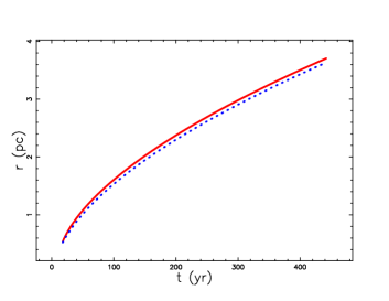
Figure 1: Numerical solution (full red line) and asymptotic approximate solution (blue dashed line) for the inverse power law with $\alpha=1.5$ Parameters as in Table 5 for Tycho.

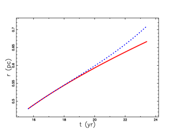
Figure 2: Numerical solution (full red line) and Taylor approximation (blue dashed line) for the inverse power law with $\alpha=1.5$. Parameters as in Table 5 for Tycho.

4.3 Presence of an exponential

The astrophysical parameters for an exponential profile of density are presented in Table 6 and the fit of the trajectory with a Taylor expansion, see Equation (40), is presented in Figure 3.

Table 6: Theoretical parameters of the SNRs for the equation of motion in the case of conservation of energy with an exponential profile of density, see Section 3.6.

Name	$t_{0}$ (yr)	$r_{0}$ (pc)	b	$v_{0}(km\,s^{-1})$	$\delta_{r}\,(\%)$	$\delta_{v}\,(\%)$	$\Delta_{10}\,v(km\,s^{-1})$
Tycho	15.83	0.48	1	30000	0.22	8.12	-27.62
Cas  A	11.91	0.365	1	30000	0.29	15.27	-43.88
Cygnus loop	5.15	0.15	0.7	30000	0.085	425	0
SN  1006	18.35	0.56	0.7	30000	0.46	178	-0.02

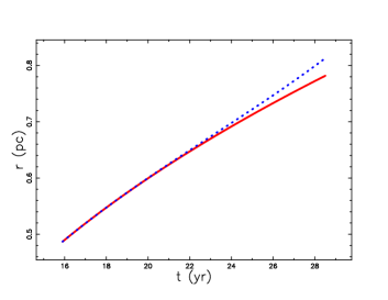
Figure 3: Numerical solution (full red line) and Taylor approximation (blue dashed line) for the exponential profile. Parameters as in Table 6 for Tycho.

The astrophysical parameters for a Gaussian profile of density are presented in Table 7 and the fit of the trajectory with a Taylor expansion, see Equation (45), is presented in Figure 4.

Table 7: Theoretical parameters of the SNRs for the equation of motion in the case of conservation of energy with a Gaussian profile of density, see Section 3.7.

Name	$t_{0}$ (yr)	$r_{0}$ (pc)	b	$v_{0}(km\,s^{-1})$	$\delta_{r}\,(\%)$	$\delta_{v}\,(\%)$	$\Delta_{10}\,v(km\,s^{-1})$
Tycho	12.89	0.395	1	30000	0.013	21.62	-0.005
Cas  A	10.95	0.335	1	30000	0.034	7.79	-3.2
Cygnus loop	3.2	0.0979	0.7	30000	0.0385	445	0
SN  1006	11.73	0.359	0.7	30000	0.087	206.2	0

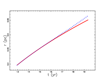
Figure 4: Numerical solution (full red line) and Taylor approximation (blue dashed line) for the Gaussian profile. Parameters as in Table 7 for Tycho.

4.4 Autogravitating medium

The astrophysical parameters for an autogravitating medium are presented in Table 8 and the fit of the trajectory with a Taylor expansion, see Equation (53), is presented in Figure 5.

Table 8: Theoretical parameters of the SNRs for the equation of motion in the case of conservation of energy with an autogravitating profile of density, see Section 3.8.

Name	$t_{0}$ (yr)	$r_{0}$ (pc)	b	$v_{0}(km\,s^{-1})$	$\delta_{r}\,(\%)$	$\delta_{v}\,(\%)$	$\Delta_{10}\,v(km\,s^{-1})$
Tycho	24.57	0.752	1.5	30000	0.019	25.1	-38.3
Cas  A	15.4	0.474	1	30000	0.03	23.3	-45.9
Cygnus loop	10.6	0.326	1	30000	0.046	403	-0.03
SN  1006	26.8	0.82	0.7	30000	0.002	174	-0.149

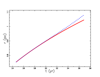
Figure 5: Numerical solution (full red line) and Taylor approximation (blue dashed line) for the autogravitating profile. Parameters as in Table 8 for Tycho.

4.5 NFW profile

The astrophysical parameters for an NFW profile of density are presented in Table 9 and the fit of the trajectory with a Taylor expansion, see Equation (60), is presented in Figure 6.

Table 9: Theoretical parameters of the SNRs for the equation of motion in the case of conservation of energy with an NFW profile of density, see Section 3.9.

Name	$t_{0}$ (yr)	$r_{0}$ (pc)	b	$v_{0}(km\,s^{-1})$	$\delta_{r}\,(\%)$	$\delta_{v}\,(\%)$	$\Delta_{10}\,v(km\,s^{-1})$
Tycho	13.3	0.408	1.5	30000	0.07	3	-34.8
Cas  A	8	0.245	1	30000	0.073	0.26	-42.3
Cygnus loop	3.43	0.1052	1	30000	0.09	338	-0.1
SN  1006	27.5	0.845	0.7	30000	0.074	136	-14.1

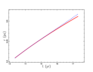
Figure 6: Numerical solution (full red line) and Taylor approximation (blue dashed line) for an NFW profile. Parameters as in Table 9 for Tycho.

5 Conclusions

The thin layer approximation in the framework of the conservation of energy is an alternative to the use of the conservation of momentum in order to find the equation of motion for a supernova remnant (SNR). In the case where the interstellar medium (ISM) has a constant density, it is possible to find the trajectory in an analytical form, see Equation (11). The case of energy conservation in a medium with variable density was also explored but an analytical trajectory was found only in the case of a medium characterized by an inverse square decrease of density, see Equation (26). The other profiles of density require a numerical integration in order to find the trajectory. A Taylor series can provide the trajectory for a short interval of time: see Figure 2 for a power law, Figure 3 for an exponential law, Figure 4 for a Gaussian law, Figure 5 for an autogravitating medium and Figure 6 for a Navarro–Frenk–White (NFW) density profile. As an astrophysical target we have chosen to reproduce 4 standard SNRs. The match between the observed and simulated radius as well as that between the observed velocity and the simulated velocity has been analysed in terms of the percentage error, see Tables 2, 3, 4, 5, 6, 7, 8 and 9. Table 10 presents in column 2 the best model for the SNRs here analysed.

Table 10: Synoptical parameters of the best model for SNRs with different density profiles.

Name	model	$t_{0}$ (yr)	$r_{0}$ (pc)	$v_{0}(km\,s^{-1})$	$\delta_{r}\,(\%)$	$\delta_{v}\,(\%)$
Tycho	inverse  square	10.44	0.32	30000	0.016	0.98
Cas  A	NFW , b=1 pc	8	0.245	30000	0.073	0.26
Cygnus loop	power law	9.96	0.3	30000	0.0443	23.29
SN  1006	power law	55.15	1.689	30000	0.07	31.53

The solution for the velocity to first order allows the insertion of the back reaction, i.e. the radiative losses, in the equation for the energy conservation, see equation (18), and as a consequence the velocity corrected to second order, see equation (19). The radiative losses allow evaluating the length at which the advancing velocity of the SNR is zero.

References

- [1] Bisnovatyj-Kogan G S and Blinnikov S I 1982 Sphericization of the remnants of an asymmetric supernova outburst in a homogeneous medium Astronomicheskii Zhurnal 59, 876
- [2] Tenorio-Tagle G and Palous J 1987 Giant-scale supernova remnants - The role of differential galactic rotation and the formation of molecular clouds A&A 186(1-2), 287
- [3] Mac Low M M and McCray R 1988 Superbubbles in disk galaxies ApJ 324, 776
- [4] McCray R A 1987 Coronal interstellar gas and supernova remnants in A Dalgarno & D Layzer, ed, Spectroscopy of Astrophysical Plasmas (Cambridge, UK: Cambridge University Press) pp 255–278
- [5] Kompaneyets A S 1960 A Point Explosion in an Inhomogeneous Atmosphere Soviet Phys. Dokl. 5, 46
- [6] Bisnovatyi-Kogan G S, Blinnikov S I and Silich S A 1989 Supernova remnants and expanding supershells in inhomogeneous moving medium Astrophysics and Space Science 154, 229
- [7] Dyson, J E and Williams, D A 1997 The physics of the interstellar medium (Bristol: Institute of Physics Publishing)
- [8] Bisnovatyi-Kogan G S and Silich S A 1998 in D Breitschwerdt, M J Freyberg and J Truemper, eds, IAU Colloq. 166: The Local Bubble and Beyond vol 506 (Berlin: Springer) pp 137–140
- [9] Padmanabhan P 2001 Theoretical astrophysics. Vol. II: Stars and Stellar Systems (Cambridge, UK: Cambridge University Press)
- [10] Chen Y, Zhang F, Williams R M and Wang Q D 2003 Supernova Remnant Crossing a Density Jump: A Thin-Shell Model ApJ 595(1), 227 (Preprint astro-ph/0306126)
- [11] De Young D S 2002 The physics of extragalactic radio sources (Chicago: University of Chicago Press)
- [12] Zaninetti L 2015 Classical and relativistic conservation of momentum flux in radio-galaxies Applied Physics Research 7, 43
- [13] Zaninetti L 2016 Classical and relativistic flux of energy conservation in astrophysical jets Journal of High Energy Physics, Gravitation and Cosmology 1, 41
- [14] Olver F W J e, Lozier D W e, Boisvert R F e and Clark C W e 2010 NIST Handbook of Mathematical Functions (Cambridge: Cambridge University Press. )
- [15] Spitzer Jr L 1942 The Dynamics of the Interstellar Medium. III. Galactic Distribution. ApJ 95, 329
- [16] Rohlfs K, ed 1977 Lectures on density wave theory vol 69 of Lecture Notes in Physics, Berlin Springer Verlag
- [17] Bertin G 2000 Dynamics of Galaxies (Cambridge: Cambridge University Press.)
- [18] Padmanabhan P 2002 Theoretical astrophysics. Vol. III: Galaxies and Cosmology (Cambridge, UK: Cambridge University Press)
- [19] Navarro J F, Frenk C S and White S D M 1996 The Structure of Cold Dark Matter Halos ApJ 462, 563 (Preprint astro-ph/9508025)
- [20] Williams B J, Chomiuk L, Hewitt J W, Blondin J M, Borkowski K J, Ghavamian P, Petre R and Reynolds S P 2016 An X-Ray and Radio Study of the Varying Expansion Velocities in Tycho Supernova Remnant ApJ Letters, 823 L32 (Preprint 1604.01779)
- [21] Patnaude D J and Fesen R A 2009 Proper Motions and Brightness Variations of Nonthermal X-ray Filaments in the Cassiopeia A Supernova Remnant ApJ 697, 535 (Preprint 0808.0692)
- [22] Chiad B T, Ali L T and Hassani A S 2015 Determination of Velocity and Radius of Supernova Remnant after 1000 yrs of Explosion International Journal of Astronomy and Astrophysics 5, 125
- [23] Uchida H, Yamaguchi H and Koyama K 2013 Asymmetric Ejecta Distribution in SN 1006 ApJ 771 56 (Preprint 1305.4489)