[2004.14838] 1 Estimation of the model parameters

Branching stochastic processes as models

of Covid-19 epidemic development

Nikolay M. Yanev

¹, Vessela K. Stoimenova², Dimitar V. Atanasov³

Abstract.

The aim of the paper is to describe two models of Covid-19 infection dynamics. For this purpose a special class of branching processes with two types of individuals is considered. These models are intended to use only the observed daily statistics to estimate the main parameter of the infection and to give a prediction of the mean value of the non-observed population of the infected individuals. Similar problems are considered also in the case when the processes admit an immigration component. This is a serious advantage in comparison with other more complicated models where the officially reported data are not sufficient for estimation of the model parameters. In this way the specific development of the Covid-19 epidemics is considered also for all countries as it is given in the specially created site http://ir-statistics.net/covid-19 where the obtained results are updated daily.

MSC-2020: Primary 92D30

Secondary 60J80; 60J85; 62P10

Key words: Codid-19, epidemiology

, branching processes, immigration, modeling, estimation.

1. Introduction.

The theory of branching processes is a powerful tool for investigation the population dynamics where the members can reproduce new members following some stochastic laws. The objects may be of different types and nature. Branching processes have serious applications in physics, chemistry, biology and medicine, demography, epidemiology, economics, computer science an so on. Basic models and analytical results are presented in some books and a lot of papers. We would like to point out the monographs $[1-8]$ among the others. Some applications of branching processes in biology and medicine are presented in $[5]$ , $[9]$ and $[10]$ . For statistical inference of branching processes one can consider $[11]$ and $[12].$ Some specific estimation problems are given in $[13]$ , $[14]$ and $[15]$ .

The aim of the present paper is to model and to estimate the development of the Covid-19 infection in the population. For this purpose a special class of branching processes with two types of infected individuals is constructed and considered day by day. In fact they are ”infected undiagnosed” vs ” infected diagnosed” following the terminology of P. Jagers (personal communication). It is proposed also a generalization of this situation assuming an immigration component. In this way we are able to use the observed data for the Covid-19 daily registered infected individuals and to estimate the main parameter of infection. In fact this parameter $m$ represents the mean value of the infected individuals by one individual per day. Using the observed statistics some methods for estimation are proposed and corresponding graphics are presented. Two models with and without immigration are compared. In this way we are able to give a prediction of the possible development of the mean value of the infected individuals.

Notice that both type processes with or without immigration have an exponential growth in the supercritical case $m>1$ but in the critical case $m=1$ and in the subcritical case $m<1$ the asymptotic behaviour is essentially different. In the critical case the mean value of the process with immigration grows linearly while for the process without immigration the mean value is constant. In the subcritical case the mean value of the immigration process converges to a positive constant but for the process without immigration the mean value goes to zero. The estimation of the immigration mean $a$ is a serious problem because this parameter cannot be estimated by the observed data and one needs additional information. Hence the processes with immigration need more careful investigation.

As it is given in the paper the proposed estimators can be applied also in the case when the processes are inhomogeneous in time. The behaviour of the estimators shows that the observed processes are able to change the criticality during the development of the epidemics. The estimated values for the main epidemical parameter $m$ vary greater than $1$ , equal (or very closed) to $1$ and even less than $1.$ Moreover it seems that the real epidemic process develops like a mixture of both type of the models with and without immigration. In this case four stages of epidemic development are available: exponential growth ( $m>1$ ), linear growth ( $m=1$ and an immigration component), non-increasing and almost stable population (due to $m=1$ or $m<1$ with an immigration component), convergence to zero (extinction of the epidemics due to $m<1$ without immigration). It is obvious that the restriction of the immigration component is very important to the limitation of the epidemic process. It seems that in some countries exist some regions which can be considered as immigration sources for the other regions and in general for the whole country. The abroad immigration plays also an important role.

The paper continues the investigations started in $[16]$ where some results for the model without immigration were presented only for Bulgaria, Italy and globally.

In the present paper as an illustration of the models with and without immigration the obtained results are presented for several countries: USA, Italy, France, Germany, Spain and Bulgaria. Additional information, reports and plots, related to this research for all countries all over the world can be found on the site http://ir-statistics.net/covid-19. The data used for the estimation of the parameters of the model are taken from European Centre for Disease Prevention and Control $[21]$ , similar to the data provided by World Health Organization $[20]$ . Since these databases are updated daily, the proposed here model is applied regularly on each new data set. Using these results one can compare the infection rate on different countries and regions on the basis of estimated growth rate. For example, on Table 3, the 10 countries with lowest and highest growth rate are shown. Even in the cases where the infection growth is less than 1, the confidence interval goes above 1, which states that there is a possibility for increasing of the infection growth in the future.

The theoretical model based on two type branching process is described in detail in Section 2. The p.g.f.’s and the mathematical expectations are obtained. Regardless of its simplicity the model has a great advantage using only the observed official data for the lab-confirmed cases. The two-type branching process assuming an additional immigration component is considered in Section 3. The estimation problems are presented in Section 4. Some conclusive remarks are given in Section 5.

Finally the estimation of the mean parameter of infection can be considered as a fast test to estimate the rate of Covid-19 epidemic in a country or a region. It can be used also as a first stage of a construction to some more complicated epidemiological models where it is not possible to estimate directly this parameter. Obviously the solution of this problem requires the collaboration of specialists in various fields as epidemiology, mathematics, medicine, microbiology, molecular biology and informatics among others.

2 Two-type branching process as model of Covid-19 population dynamics.

Assume that the epidemic process of infection begins with some finite number of immigrants and then the process of immigration is isolated under the quarantine.

To describe this situation we can consider a two type branching process $\{Z_{1}(n),Z_{2}(n)\}$ where type $T_{1}$ are infected (but still healthy) individuals who don’t know that they are Covid-19 infected and type $T_{2}$ of discovered with Covid-19 virus individuals (and this is the data we use). Every individual of type $T_{1}$ (infected) produces per day a random number of new individuals of type $T_{1}$ (infected) or only one individual of type $T_{2}$ (more precisely, in this case the individual type $T_{1}$ is transformed into an individual type $T_{2}).$ Note that $T_{2}$ is a final type, i.e. the individuals of this type don’t take part in the further evolution of the process because they are isolated under the quarantine.

Let $\mathbf{\xi}_{1}=(\xi_{1}^{(1)},\xi_{2}^{(1)})$ be the offspring vector of type $T_{1}.$ Then the offspring joint probability generating function (p.g.f.) of type $T_{1}$ can be defined as follows:

$(1)$ $\ \ h_{1}(s_{1},s_{2})=\mathbf{E(}s_{1}^{\xi_{1}^{(1)}}s_{2}^{\xi_{2}^{(1)}})=p_{0}+\sum_{j=1}^{k}p_{j}s_{1}^{j}+qs_{2},|$ $s_{1}|\leq 1,|s_{2}|\leq 1,$

where $q=1-\sum_{j=0}^{k}p_{j},$ $h_{1}(1,1)=1.$

Obviously $h_{2}(s_{1},s_{2})\equiv 1$ because the type $T_{2}$ has $(0,0)$ offspring.

Note that $p_{0}$ is the probability that type $T_{1}$ goes out of the reproduction process (the individual becomes healthy or goes out of the country, i.e. emigrates), $p_{j}$ is the probability to produce new $j$ infected individuals of type $T_{1}$ and $q$ is the probability that the individual type $T_{1}$ is confirmed ill (or dead). In other words, $q=\mathbf{P}\{T_{1}\rightarrow T_{2}\},$ i.e. with probability $q$ an individual of type $T_{1}$ is transformed into an individual of type $T_{2}.$ Then from $(1)$ we can obtain also that the marginal p.g.f. are
$(2)$ $\ \ \ \mathbf{E(}s_{1}^{\xi_{1}^{(1)}})=h_{1}(s_{1},1)=p_{0}+\sum_{j=1}^{k}p_{j}s_{1}^{j}+q=1-\sum_{j=1}^{k}p_{j}(1-s_{1}^{j}),$
$(3)$ $\ \ \ \mathbf{E(}s_{2}^{\xi_{2}^{(1)}})=h_{1}(1,s_{2})=1-q+qs_{2}.$

If we assume that $Z_{1}(0)>0$ and $Z_{2}(0)=0$ then for $n=1,2,...$
$(4)$ $Z_{1}(n)=\sum_{j=1}^{Z_{1}(n-1)}\xi_{1}^{(1)}(n;j),$ $Z_{2}(n)=\sum_{j=1}^{Z_{1}(n-1)}\xi_{2}^{(1)}(n;j),$
where the vectors $\{(\xi_{1}^{(1)}(n;j),\xi_{2}^{(1)}(n;j)\}$ are independent and identically distributed (iid) as $(\xi_{1}^{(1)},\xi_{2}^{(1)}).$

The recurrent formula $(4)$ defines two-type branching process $\{(Z_{1}(n),Z_{2}(n)),n=0,1,2,...\}.$ Notice that $Z_{1}(n)$ is the total number of individuals (type $T_{1}$ ) in the $n$ -th day infected by the individuals of the $(n-1)$ -th day; $Z_{2}(n)$ is the total number of the registered Covid-19 individuals (type $T_{2}$ ) in the $n$ -th day. The process starts with $Z_{1}(0)$ infected individuals, where $Z_{1}(0)$ can be an integer-valued random variable with a p.g.f. $h_{0}(s)=Es^{Z_{0}}=\sum_{k=1}^{K}p_{0k}s^{k},$ $|s|\leq 1$ , or $Z_{0}=N$ for some integer value, $N=1,2,...$ . The random variable $\xi_{1}^{(1)}(n;j)$ is the number of individuals of type $T_{1}$ in the $n$ -th day infected by the $j$ -th individual of type $T_{1}$ from the $(n-1)$ -th day, $j=1,2,...,Z_{1}(n-1)$ . Similarly the random variable $\xi_{2}^{(1)}(n;j)$ is the number of the confirmed infected individuals (type $T_{2})$ in the $n$ -th day transformed by the $j$ -th infected individual type $T_{1}$ from the $(n-1)$ -th day, $j=1,2,...,Z_{1}(n-1)$ .

Note that $\mathbf{P}\{\xi_{2}^{(1)}(n;j)=0\}=1-q$ and $\mathbf{P}\{\xi_{2}^{(1)}(n;j)=1\}=q.$ Hence $Z_{2}(n)\in Bi(Z_{1}(n-1,q),$ i.e.
$\mathbf{P}\{Z_{2}(n)=i|Z_{1}(n-1)=l\}=(_{i}^{l})q^{i}(1-q)^{l-i},i=0,1,...,l;l=0,1,2,...$

In other words the probability $q$ can be interpreted as a proportion of the confirmed individuals in the day $n$ among all infected individuals in the day $n-1$ .

Let $h_{0}(s)=\mathbf{E}s^{Z_{1}(0)},$ $F_{1}(n;s)=\mathbf{E(}s^{Z_{1}(n)}),$ $F_{2}(n;s)=\mathbf{E(}s^{Z_{2}(n)}).$ Introduce the following p.g.f.
$(5)$ $\ \ \ h^{\ast}(s)=h_{1}(s,1)=q+p_{0}+\sum_{j=1}^{k}p_{j}s^{j},$ $\widetilde{h}(s)=h_{1}(1,s)=1-q+qs.$

Then it is not difficult to check that for $n=0,1,2,...,$ we are able to obtain the p.g.f. of the process:
$(6)$ $\ \ \ F_{1}(n;s)=\mathbf{E(}s^{Z_{1}(n)})=F_{1}(n-1;h^{\ast}(s))=F_{1}(0;h_{n}^{\ast}(s))$

$\ \ \ \ \ \ \ \ \ \ \ \ \ \ =h_{0}(h^{\ast}(h^{\ast}(...(h^{\ast}(s))...))),$
$(7)$ $\ \ \ F_{2}(n;s)=\mathbf{E(}s^{Z_{2}(n)})=F_{1}(n-1;\widetilde{h}(s))=F_{1}(0;\widetilde{h}_{n}(s))$

$\ \ \ \ \ \ \ \ \ \ \ \ \ \ =h_{0}(\widetilde{h}(\widetilde{h}(...(\widetilde{h}(s))...))),\newline$ where the p.g.f. $h_{n}^{\ast}(s)$ and $\widetilde{h}_{n}(s)$ are obtained after $n$ compositions of the p.g.f. $h^{\ast}(s)$ and $\widetilde{h}(s)$
$(8)$ $\ \ h_{n}^{\ast}(s)=h^{\ast}(h^{\ast}(...(h^{\ast}(s))...)),h_{0}^{\ast}(s)=s;\widetilde{h}_{n}(s)=\widetilde{h}(\widetilde{h}(...(\widetilde{h}(s))...)),\widetilde{h}_{0}(s)=s.$

Let $m=\frac{d}{ds}h^{\ast}(s)|_{s=1}=\mathbf{E}\xi_{1}^{(1)}=\sum_{j=1}^{k}jp_{j}$ be the mean value of the new infected individuals by one infected individual. Note that $\frac{d}{ds}\widetilde{h}(s)|_{s=1}=\mathbf{E}\xi_{2}^{(1)}=q$ is the mean value of the registered infected individuals by one infected individual. Introduce also $m_{0}=\mathbf{E}Z_{1}(0)=\frac{d}{ds}h_{0}(s)|_{s=1}.$ Therefore
$(9)$ $\ \ M_{1}(n)=\mathbf{E}Z_{1}(n)=m_{0}m^{n},n=0,1,2,...,$
$(10)$ $\ \ M_{2}(n)=\mathbf{E}Z_{2}(n)=q\mathbf{E}Z_{1}(n-1)=qm_{0}m^{n-1},n=1,2,...;\mathbf{E}Z_{2}(0)=0.$

Notice that the asymptotic behaviour of the process depends essentially of parameter $m.$ Especially, if $m>1$ (supercritical case) then the mean value of the infected individuals $M_{1}(n)$ grows exponentially, in the critical case $m=1$ it is a constant and for $m<1$ (subcritical case) $M_{1}(n)\rightarrow 0$ as $n\rightarrow\infty.$

We will use these results to present in the next section a more complicated model with immigration.

Note that we can observe only $Z_{2}(1),Z_{2}(2),...,Z_{2}(n).$ What can be estimated with these observations?

Note first that $\frac{\mathbf{E}Z_{2}(n+1)}{\mathbf{E}Z_{2}(n)}=m.$ Hence we can consider
$(11)$ $\ \ \ \ \ \widehat{m}_{n}=\frac{Z_{2}(n+1)}{Z_{2}(n)},n=1,2,....,$
as an estimator of the parameter $m$ (similar to Lotka-Nagaev estimator for the classical BGW branching process). It is possible to use also the following Harris type estimator
$(12)$ $\widetilde{m}_{n}=\sum_{i=2}^{n+1}Z_{2}(i)/\sum_{j=1}^{n}Z_{2}(j),n=1,2,....,$
or Crump and Hove type estimators
$(13)$ $\overline{m}_{n,N}=\sum_{i=n+1}^{n+N}Z_{2}(i)/\sum_{j=n}^{n+N-1}Z_{2}(j),n=1,2,...;N=1,2,....$

See $[12]$ for more details.

Estimating $m$ we are able to predict the mean value of the infected (non observed) individuals in the population. In the case when we assume that $Z_{1}(0)=1$ then $M_{1}(n)=\mathbf{E}Z_{1}(n)$ can be approximated respectively by $\widehat{m}_{n}^{n}$ , or $\widetilde{m}_{n}^{n}$ , or $\overline{m}_{n,N}^{n}.$ In fact it means that we can obtain three types of estimators
$(14)$ $\widehat{M}_{1}(n)=$ $\widehat{m}_{n}^{n},$ $\widetilde{M}_{1}(n)=$ $\widetilde{m}_{n}^{n}$ and $\overline{M}_{1}(n)=\overline{m}_{n,N}^{n}.$

In other words we could say that we have at least three prognostic lines. Therefore if we have the observations $(Z_{2}(1),Z_{2}(2),...,Z_{2}(n))$ over the first $n$ days, we are able to predict the mean value of the infected individuals for the next $k$ days by the relations:
$(15)$ $\widehat{M}_{1}(n+k)=$ $\widehat{m}_{n}^{n+k},$ $\widetilde{M}_{1}(n+k)=$ $\widetilde{m}_{n}^{n+k}$ and $\overline{M}_{1}(n+k)=\overline{m}_{n,N}^{n+k},$ $k=1,2,...$

We are able to estimate also the proportion $\alpha(n)$ of the registered infected individuals among the population in the $n$ -th day. Then we can obtain the following three types of estimators: $\widehat{\alpha}(n)=$ $Z_{2}(n)/\{Z_{2}(n)+\widehat{M}_{1}(n)\},$ $\widetilde{\alpha}(n)=Z_{2}(n)/\{Z_{2}(n)+\widetilde{M}_{1}(n)\},$ $\overline{\alpha}(n)=Z_{2}(n)/\{Z_{2}(n)+\overline{M}_{1}(n)\}.$

All obtained estimators will be presented by the observed registered lab-confirmed cases. The quality of the estimation, however, depends on the representativeness of the sample due to the specifics of the data collection in each country.

Remark 1. In fact our model $(4)$ can be generalized as non-homogeneous in time. In this case $m(l)=\frac{d}{ds}h^{\ast}(l;s)|_{s=1}=\mathbf{E}\xi_{1}^{(1)}(l)=\sum_{j=1}^{k}jp_{j}(l)$ will be the mean value of the new infected individuals by one infected individual in the day $l=1,2,...$ . Therefore instead $(9)$ we obtain
$(16)$ $\ \ M_{1}(n)=\mathbf{E}Z_{1}(n)=m_{0}\Pi_{l=1}^{n}m(l),n=0,1,2,....$

Notice that in this case $\frac{\mathbf{E}Z_{2}(n+1)}{\mathbf{E}Z_{2}(n)}=m(n).$ Hence we can use $(11)-(13)$ to estimate $M_{1}(n)$ from $(16).$ Therefore
$(17)$ $\widehat{M}_{1}(n)=\Pi_{l=1}^{n}$ $\widehat{m}_{l},$ $\widetilde{M}_{1}(n)=$ $\Pi_{l=1}^{n}\widetilde{m}_{l},n=1,2,..$

3. The two-type branching process with immigration as model of Covid-19 epidemic development.

The model considered in Section 2 assumes that the process of infection begins with some random number of infected immigrants and then the immigration process is bounded and it is not essential for the Covid-19 population dynamics. But in some cases the role of the immigration process cannot be negligible. That is why we will introduce random variables $\{I_{n}\},$ where $I_{n}$ gives the number of infected immigrants in the $n-th$ day which take part in the process of infection. We will assume first that $\{I_{n}\}$ are iid r.v. with a p.g.f.
$(18)\ \ \$ $g(s)=\mathbf{E}s^{I_{n}}=\sum_{k=0}^{l}g_{k}s^{k},|s|\leq 1.$

Then instead of $(4)$ we will consider the following branching process with immigration
$(19)$ $Y_{1}(n)=\sum_{j=1}^{Y_{1}(n-1)}\xi_{1}^{(1)}(n;j)+I_{n},$ $Y_{2}(n)=\sum_{j=1}^{Y_{1}(n-1)}\xi_{2}^{(1)}(n;j),n=1,2,...,$
where the vectors $\{(\xi_{1}^{(1)}(n;j),\xi_{2}^{(1)}(n;j)\}$ are independent and identically distributed as $(\xi_{1}^{(1)},\xi_{2}^{(1)})$ with p.g.f. $(1)-(3)$ and they are also independent of $\{I_{n}\}.$ We can assume that $Y_{1}(0)>0$ is some random variable independent of $\{(\xi_{1}^{(1)}(n;j),\xi_{2}^{(1)}(n;j)\}$ and $\{I_{n}\},$ and also the case $\ Y_{2}(0)=0.$ Another possible assumption is $Y_{1}(0)=Y_{2}(0)=0,$ which means that in fact the process starts with the first real immigrants.

Interpretation: $Y_{1}(n)$ is the total number of individuals (type $T_{1}$ ) in the $n$ -th day infected by the individuals of the $(n-1)$ -th day plus the new infected immigrants $I_{n}$ ; $Y_{2}(n)$ is the total number of the officially registered infected individuals (type $T_{2}$ ) in the $n$ -th day.

Then it is not difficult to check that for $n=0,1,2,...,$ we are able to obtain from $(18)$ and $(19)$ the p.g.f.’s of the process:
$\ \ \ \ \ \ G_{1}(n;s)=\mathbf{E(}s^{Y_{1}(n)})=g(s)G_{1}(n-1;h^{\ast}(s))=f(h_{n}^{\ast}(s))\Pi_{k=0}^{n-1}g(h_{k}^{\ast}(s)),$
$\ \ \ \ \ \ G_{2}(n;s)=\mathbf{E(}s^{Y_{2}(n)})=G_{1}(n-1;\widetilde{h}(s))$

$\ \ \ \ \ \ \ \ \ \ \ \ \ =g(\widetilde{h}(s))G_{1}(n-2;h^{\ast}(\widetilde{h}(s)))=f(h_{n-2}^{\ast}(\widetilde{h}(s)))\Pi_{k=0}^{n-1}g(h_{k}^{\ast}(\widetilde{h}(s))),\newline$ where the p.g.f. $h_{k}^{\ast}(s)$ and $\widetilde{h}_{k}(s)$ are obtained after $k$ iterations of the p.g.f. $h^{\ast}(s)$ and $\widetilde{h}(s)$ as it is given in $(8)$ and
$f(s)=\mathbf{E}s^{Y_{1}(0)}=\sum_{k=0}^{N}f_{k}s^{k},|s|\leq 1.$

Notice that if we assume that $Y_{1}(0)=0$ then $f(s)\equiv 1$ and
$(20)$ $G_{1}(n;s)=\Pi_{k=0}^{n-1}g(h_{k}^{\ast}(s)),$ $G_{2}(n;s)=\Pi_{k=0}^{n-2}g(h_{k}^{\ast}(\widetilde{h}(s))).$

From $(18)$ we can introduce the immigration mean $a=\mathbf{E}I_{n}=\frac{d}{ds}g(s)|_{s=1}=\sum_{k=0}^{l}kg_{k}$ . Then from $(18)-(20)$ it is not difficult to obtain that for $n=1,2,...$
$(21)$ $A_{1}(n)=\mathbf{E}Y_{1}(n)=mA_{1}(n-1)+a=a\sum_{k=0}^{n-1}m^{k},$
$(22)$ $A_{2}(n)=\mathbf{E}Y_{2}(n)=qA_{1}(n-1)=qa\sum_{k=0}^{n-2}m^{k},$
where it is assumed that $A_{1}(0)=\mathbf{E}Y_{1}(0)=0$ and the parameters $m$ and $q$ are well defined in Section 2 by $(5).$

Hence from $(21)$ and $(22)$ one has
$(23)$ $A_{1}(n)=a(m^{n}-1)/(m-1),m\neq 1,$ and $A_{1}(n)=an,m=1,$
$(24)$ $A_{2}(n)=qa(m^{n-1}-1)/(m-1),m\neq 1,$ and $A_{2}(n)=qa(n-1),m=1$

Therefore by $(23)$ and $(24)$ one obtains as $n\rightarrow\infty$
$A_{1}(n)\sim am^{n}/(m-1),m>1;A_{1}(n)=an,m=1;A_{1}(n)\rightarrow a/(1-m),m<1,$
$A_{2}(n)\sim qam^{n-1}/(m-1),m>1;A_{2}(n)\sim qan,m=1;A_{1}(n)\rightarrow\frac{qa}{1-m},m<1.$

In the general case $A_{1}(0)=\mathbf{E}Y_{1}(0)=M_{0}>0$ and instead of $(19)$ and $(20)$ one has
$(25)$ $A_{1}(n)=M_{0}m^{n}+a\sum_{k=0}^{n-1}m^{k},$
$(26)$ $A_{2}(n)=q(M_{0}m^{n-1}+a\sum_{k=0}^{n-2}m^{k}).$

We would like to point out once again that we can observe only the statistics $Y_{2}(1),Y_{2}(2),...,Y_{2}(n)$ and we have to use for estimation only these observations.

Notice first that for $m\geq 1$ we obtain $\lim_{n\rightarrow\infty}\frac{\mathbf{E}Y_{2}(n+1)}{\mathbf{E}Y_{2}(n)}=m.$ Hence for large enough $n$ we can consider
$(27)$ $\ \ \ \ \ \widehat{m}_{n}=Y_{2}(n+1)/Y_{2}(n)$
as an estimator of the parameter $m$ (similar to Lotka-Nagaev estimator for the classical BGW branching process). It is possible to use also for $m>1$ and large enough $n$ the following Harris type estimator
$(28)$ $\widetilde{m}_{n}=\sum_{i=2}^{n+1}Y_{2}(i)/\sum_{j=1}^{n}Y_{2}(j)$
or Crump and Hove type estimators
$(29)$ $\overline{m}_{n,t}=\sum_{i=n+1}^{n+t}Y_{2}(i)/\sum_{j=n}^{n+t-1}Y_{2}(j).$

See $[12]$ for more details.

Estimating $m>1$ we are able to predict the mean value of the infected (non observed) individuals in the population. In the case when we assume that the process begins with the first immigrants then $A_{1}(n)=\mathbf{E}Y_{1}(n)$ can be approximated using the estimators $(27)-(29).$

The problem is how to estimate the immigration mean $a$ . First of all there is an special case when $a=m$ . Then using $(23)$ and $(24)$ with the Harris estimator we have
$(30)$ $\widetilde{A}_{1}(n)=\widetilde{m}_{n}(\widetilde{m}_{n}^{n}-1)/(\widetilde{m}_{n}-1),m>1;$ $\widetilde{A}_{1}(n)=\widetilde{m}_{n}n,m=1.$

In general we have to use some additional information. For example, if we can observe $\{I_{k}\}$ then we can apply the estimator $a_{n}^{\ast}=n^{-1}\sum_{k=1}^{n}I_{k}.$ Hence
$(31)$ $\widetilde{A}_{1}(n)=a_{n}^{\ast}(\widetilde{m}_{n}^{n}-1)/(\widetilde{m}_{n}-1),m>1;$ $\widetilde{A}_{1}(n)=a_{n}^{\ast}n,m=1.$

One can proceed similarly for the other estimators $\widehat{m}_{n}^{n}$ and $\overline{m}_{n,N}^{n}.$

Remark 2. Similarly as it is shown in Remark 1 from Section 2 the model $(19)$ can be generalized in the case with non-homogeneous in time offspring distributions. In this case $m(l)=\frac{d}{ds}h^{\ast}(l;s)|_{s=1}=\mathbf{E}\xi_{1}^{(1)}(l)=\sum_{j=1}^{k}jp_{j}(l)$ will be the mean value of the new infected individuals by one infected individual in the day $l=1,2,...$ . Therefore instead $(25)$ we obtain
$(32)$ $\ A_{1}(n)=\mathbf{E}Y_{1}(n)=M_{0}\Pi_{l=1}^{n}m(l)+a\sum_{k=0}^{n-1}\Pi_{l=1}^{k}m(l).$

3. Estimating of the main parameter and some predictions.

Recall that both type processes with or without immigration have exponential growth in the supercritical case $m>1$ . In the critical case $m=1$ and in the subcritical case $m<1$ the asymptotic behaviour is essentially different. In the critical case the mean value of the process with immigration grows linearly while for the process without immigration the mean value is constant. In the subcritical case the mean value of the immigration process converges to a positive constant but for the process without immigration the mean value limit is equal to zero. The estimation of the immigration mean $a$ cannot be estimated by the observed statistics and we need some additional information.

We would like to point out once again that the considered in Section 2 model is versatile but the application in each country is specific because it depends essentially on the official data from the country. The plots and tables below illustrate well some specific details for different countries as well as the common trend.

The data used for the estimation of the parameters of the model come from European Centre for Disease Prevention and Control $[21]$ .

We will consider first the process without immigration. Note that the observed data is the number of the newly (daily) registered individuals denoted by $Z_{2}(n)$ . The data about the new number of infected individuals (denoted by $Z_{1}(n)$ ) is unobservable. The initial number $m_{0}=EZ_{1}(0)$ is also unknown. Here $n$ is the corresponding day from the beginning of the infection.

The estimation of the parameters of the defined model can be summarized in the following steps.

1.

On the basis of each sample $Z_{2}(1),\dots,Z_{2}(s)$ , $s=1,\dots,n$ , the mean numbers of the new infected individuals by one infected individual is estimated by the considered above estimators but we present only the results for Harris type estimator.
2.

The mean values of the expected number of nonregistered infected individuals are calculated for the Harris estimator as $M_{1}(s+k)=m_{0}m^{s+k}=M_{1}(s)m^{k}$ . Here, instead of $m_{0}$ the value of $M_{1}(s)$ is estimated by the registered contaminated individuals in day $s$ . For the purpose of the study, the value of $s$ is set to 20 days before the end of observed data, i.e. $s=n-20$ .
3.

The proportion $\alpha(n)$ of the registered contaminated individuals among the population of all infected in the $n$ -th day is estimated by the formula $\widetilde{\alpha}(n)=Z_{2}(n)/\{Z_{2}(n)+\widetilde{M}_{1}(n)\}$ .
4.

The expected number of individuals in the model with immigration $A_{1}(n)=\mathbf{E}Y_{1}(n)$ is calculated using equation $(25)$ , based on the Harris estimator, calculated above.
5.

The obtained results are presented with 95 % confident intervals.

Firstly, we will demonstrate the approach described above by the data of the reported laboratory-confirmed COVID-19 daily cases for USA provided by the European Centre for Disease Prevention and Control $[21]$ (the data are retrieved on 02.05.2020).

Table 1 represents the estimated model parameters for the last 5 days of the available data set. Every row in the table represents the Harris estimate $\tilde{m}_{n}$ , as well as it’s 95 % confidence interval ( $CI_{l}$ - $CI_{r}$ ), the proportion of the registered infected individuals $\alpha(n)$ and the expected values of the non-confirmed cases $M_{1}$ ( or $A_{1}$ for the process with immigration) , based on $n-k$ observations, i.e. $Z_{2}(1),...,Z_{2}(n-k);k=0,...,4$ .

$k$	$\tilde{m}_{(n-k)}$	Conf. interval	$\alpha$	$M_{1}(n-k)$	$A_{1}(n-k)$
4	1.0213	0.9828 - 1.0598	0.38596	44651	53194
3	1.0315	0.9918 - 1.0712	0.38562	59410	70771
2	1.0246	0.9771 - 1.072	0.35219	32352	38548
1	1.0545	1.0048 - 1.1041	0.38064	43190	51455
0	1.0286	0.9794 - 1.0777	0.36665	36883	43945

Table 1: Estimation of the model parameters

The following figures Figure 1 - 6 represent the parameters of the process for the USA data.

Refer to caption — Figure 1: Number of the daily reported laboratory-confirmed cases

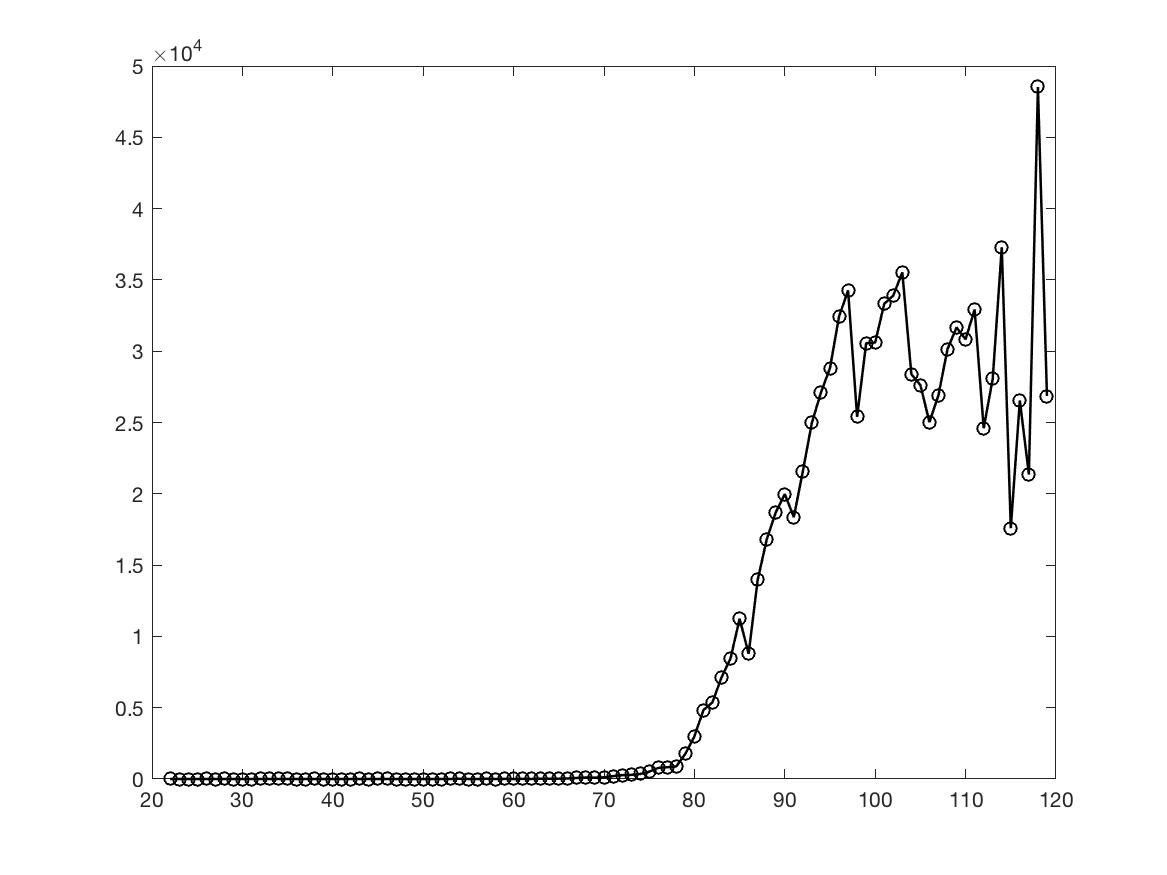
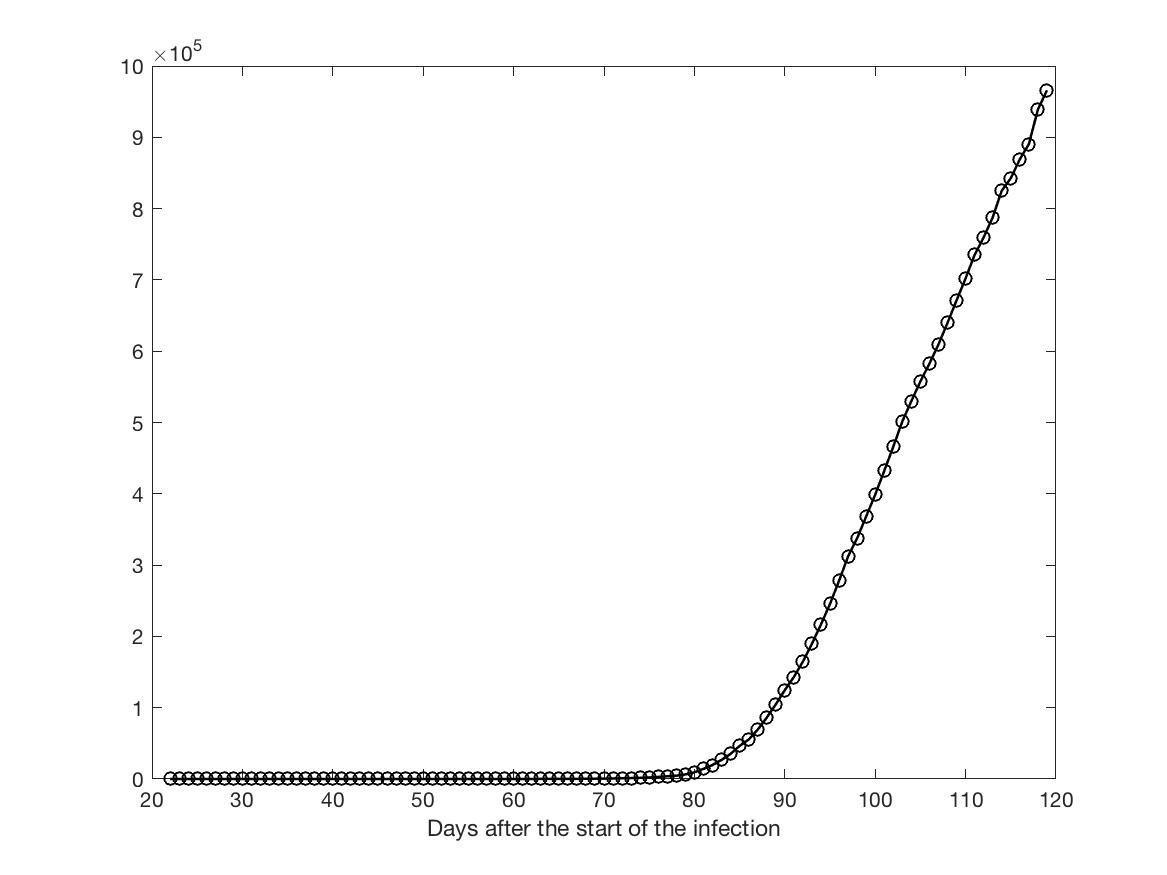
Figure 1 shows the increments $Y_{2}(n)$ - the number of the daily reported laboratory-confirmed COVID-19 cases. The related cumulative values (the number of the total registered $\sum_{i=1}^{n}Y_{2}(i)$ ) are presented on Figure 2 exhibiting a strong exponential growth.

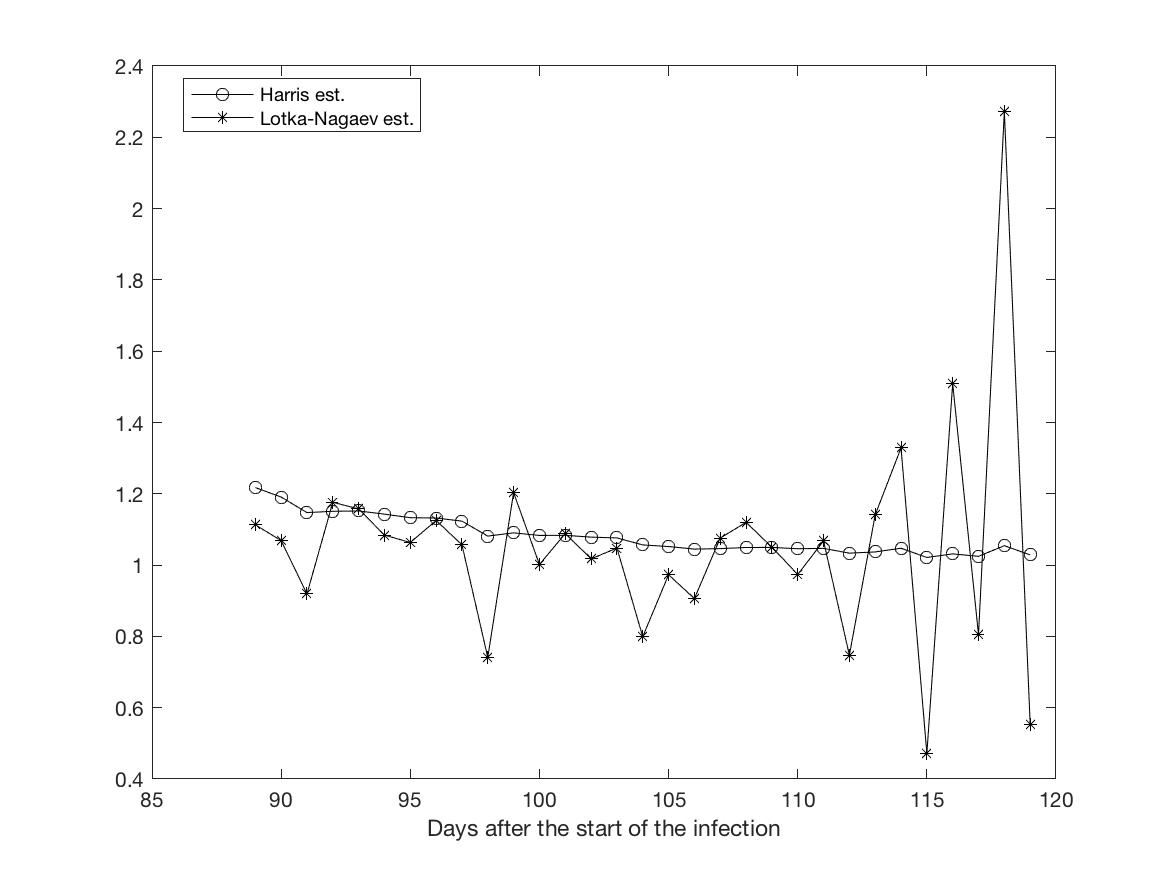
A comparison between the Harris type and Lotka-Nagaev type estimators of the growth rate (the mean value of the newly infected individuals by one infected individual) can be seen on Figure 3. After the initially large estimated values it stabilizes below 1.1, which is determined by the branching processes theory as a slightly supercritical process. This corresponds to the exponential growth shown above. The next results shows that the Harris type estimator has more stable behaviour than the Lotka-Nagaev type estimator.

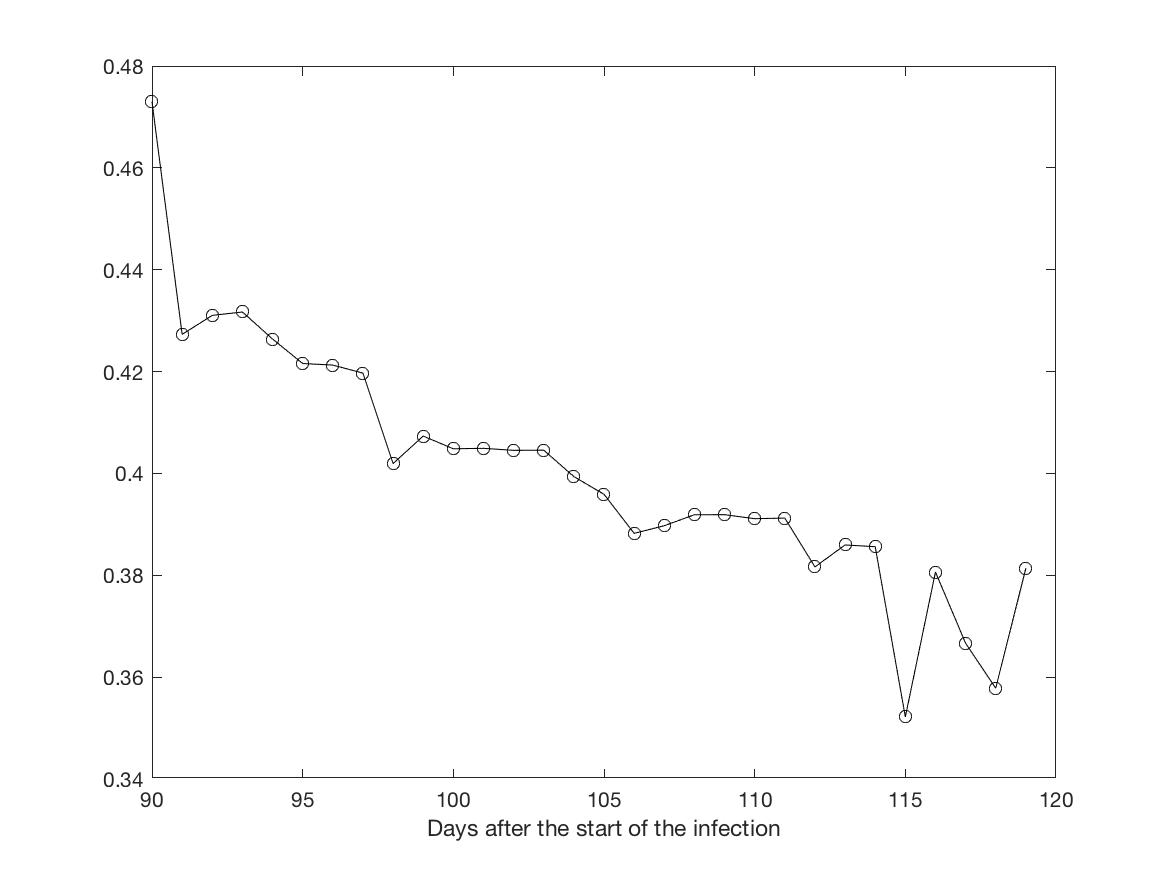
The estimates of the proportion of the officially registered lab-confirmed cases among all infected in the population can be seen on Figure 4. During the most recent days their values are approximately 0.8. This means that nearly 80% of the infected individuals have been tested, confirmed and registered.

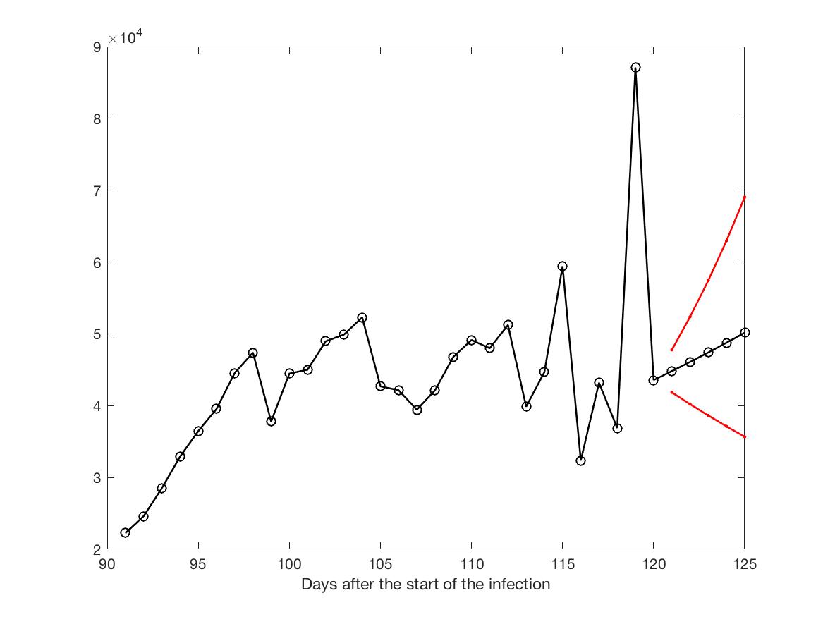
On Figure 5 the expected number of the nonregistered infected individuals by days can be seen. The last 5 points on the graph represent the 95% confidence interval for the forecast.

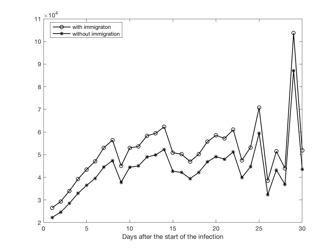
The expected number of the nonregistered infected individuals in both cases - with and without immigration, are compared on Figure 6.

Similar results for all countries in the world are available at our specially constructed site http://ir-statistics.net/covid-19. The data is provided daily by the European Centre for Disease Prevention and Control $[21]$ . The results are updated every 24 hours.

The last 5 days results for Italy, Germany, France, Spain and Bulgaria can be compared on Table 2 (the data are retrieved on 02.05.2020).

Country	$k$	$\tilde{m}_{(n-k)}$	Conf. interval	$\alpha$	$M_{1}(n-k)$	$A_{1}(n-k)$
Italy	4	1.0183	0.9641 - 1.0725	0.2189	8046	8641
	3	1.0141	0.9604 - 1.0678	0.2397	8655	9293
	2	1.0159	0.9626 - 1.0692	0.2608	9549	10249
	1	1.0122	0.9592 - 1.0651	0.2332	8699	9339
	0	1.0119	0.9596 - 1.0642	0.2458	9265	9944
France	4	1.01550	0.8575 - 1.1735	0.2589	5871	6713
	3	1.0138	0.8582 - 1.1694	0.2828	6764	7731
	2	1.0147	0.8615 - 1.1677	0.2430	5689	6506
	1	1.0125	0.8617 - 1.1633	0.2303	5522	6316
	0	1.0037	0.8551 - 1.1523	0.2365	5724	6546
Spain	4	1.0155	0.9340 - 1.0969	0.2191	11944	13471
	3	1.0138	0.9334 - 1.0942	0.1927	11006	12413
	2	1.0145	0.9352 - 1.0938	0.2064	11734	13234
	1	1.0084	0.9302 - 1.0865	0.1953	11401	12858
	0	1.0000	0.9229 - 1.0770	0.1999	11779	13284
Germany	4	1.0161	0.8954 - 1.1368	0.1735	8499	9219
	3	1.0158	0.8966 - 1.1349	0.1944	9265	10047
	2	1.0137	0.8963 - 1.1310	0.1977	9543	10348
	1	1.0114	0.8958 - 1.1270	0.1956	9605	10415
	0	1.0066	0.8926 - 1.1205	0.1825	9202	9979
Bulgaria	4	1.0482	0.8672 - 1.2291	0.2609	40	90
	3	1.0693	0.8737 - 1.2650	0.3328	92	149
	2	1.0811	0.8922 - 1.2701	0.3319	99	156
	1	1.0480	0.8637 - 1.2322	0.2917	177	244
	0	1.0409	0.8641 - 1.2177	0.2610	258	335

Table 2: Estimation of the model parameters

The value of the proportion of the registered infected individuals is considerably higher in USA and France than in Germany and Italy, while countries with a longer infection period observe relatively small values of the Harris estimator of the mean value of the number of the confirmed infected individuals by one infected individual. Even more, the lower boundary of the confidence interval for the Harris estimator falls beneath the value of 1.

Using the same data set one can compare the infection rate for different countries and regions on the basis of the estimated growth rate. For example, on Table 3, the 10 countries with lowest and highest growth rate are shown. Even in the cases where the infection growth is less than 1, the upper bound of the confidence interval goes above 1, which states that there is a possibility that the infection growth will increase in the future.

In the countries, where the infection is growing, the growth rate is isoclinically above 1, even though the lower boundary of the confidence interval is less than 1. It is usually due to the small number of observed infected individuals.

Country	$\tilde{m}_{(n-k)}$	Conf. interval
Anguilla	0.3333	0.0666 - 0.6000
Faroe Islands	0.6149	0.2740 - 0.9559
British Virgin Islands	0.6666	0.41718 - 0.9161
United States Virgin Islands	0.6909	0.2338 - 1.148
Greenland	0.8181	0.2371 - 1.3992
Seychelles	0.8181	0.40229 - 1.2341
Bhutan	0.8571	0.7513 - 0.9629
Mauritania	0.8571	0.43516 - 1.2791
Saint Kitts and Nevis	0.8666	0.3245 - 1.4088
Saint Lucia	0.8666	-0.0322 - 1.7656
Chad	1.1250	0.5820 - 1.6679
Sri Lanka	1.1320	0.8096 - 1.4545
Jamaica	1.1410	0.5097 - 1.7722
Cape Verde	1.1556	0.3000 - 3.3325
Equatorial Guinea	1.2009	0.3000 - 5.1401
Ghana	1.2103	0.24158 - 2.1791
Palestine	1.4269	0.300 - 3.2266
Eswatini	1.4500	0.7094 - 2.1906
Maldives	1.5474	0.7273 - 2.3676
Ecuador	2.0316	0.4205 - 3.6426

Table 3: Comparison of the growth rate

5. Concluding remarks.

First of all the estimation of the mean value of reproduction $m$ allows us to classify the contamination process as supercritical ( $m>1$ ), critical ( $m=1$ ) and subcritical ( $m<1$ ). Recall that both type processes with or without immigration have exponential growth in the supercritical case $m>1$ . In the critical case $m=1$ and in the subcritical case $m<1$ the asymptotic behaviour is essentially different. In the critical case the mean value of the process with immigration grows linearly while for the process without immigration the mean value is constant. In the subcritical case the mean value of the immigration process converges to a positive constant but for the process without immigration the mean value limit is equal to zero.

Finally the estimating of the mean parameter of infection can be considered as a first stage to construction of a more complicated epidemiological model. As an example, one can use a branching process with random migration considered in $[17-19]$ or some other model of controlled branching processes (see $[8]$ ). But for a general pandemic model the collaboration with specialists of epidemiology, mathematics, medicine, microbiology, molecular biology and informatics is absolutely necessary for the application of all information about Covid-19 phenomenon.

Remark 3. For more detailed investigation and simulation the following models can be applied in the considered situation:

$(\mathbf{i)}$ $h^{\ast}(s)=q+p_{0}+p_{1}s+p_{2}s^{2}+...+p_{k}s^{k},$ where $q=1-\sum_{j=0}^{k}p_{j}$ and $p_{j},j=0,1,...,k,$ can be specially chosen for $k=2,3,4,5,6,7,8.$

$(\mathbf{ii)}$ $h^{\ast}(s)=q+p_{0}+\sum_{k=1}^{\infty}(1-p)p^{k}s^{k}=q+p_{0}+(1-p)ps)/(1-ps),$ where $q+p_{0}=1-p.$ It is possible to consider also the restricted geometrical distribution up to some $k=2,3,4,5,6,7,8.$

$\mathbf{(iii)}$ $h^{\ast}(s)=q+p_{0}+\sum_{k=1}^{\infty}e^{-\lambda}\frac{\lambda^{k}}{k!}s^{k}=q+p_{0}+e^{-\lambda(1-s)}-e^{-\lambda},$ where $q+p_{0}=e^{-\lambda}.$ Similarly it is possible to consider also the restricted Poisson distribution up to some $k=2,3,4,5,6,7,8.$

Note that the parameters of these distributions can be set in the manner that $\frac{d}{ds}h^{\ast}(s)|_{s=1}$ is equal to $\widehat{m}_{n}$ , or $\widetilde{m}_{n}$ , or $\overline{m}_{n,N}.$ Then with this individual distributions it is possible to simulate the trajectories of the non-observed process of infection for further studies.

Additional information, reports and plots, related to this research can be found on http://ir-statistics.net/covid-19. The presented results are updated every day following the new data which are provided day by day from European Centre for Disease Prevention and Control $[21].$

Acknowledgements

The authors would like to express their gratitude to P. Jagers, C. Athreya, E. Yarovaya, M. Molina, E. Waymire and all the colleagues of the ”branching community” for the useful discussion and suggestions on the first paper $[16]$ on Covid-19 topic.

The research was partially supported by the National Scientific Foundation of Bulgaria at the Ministry of Education and Science, grant No KP-6-H22/3 and by the financial funds allocated to the Sofia University ”St. Kliment Ohridski”, grant N: 80-10-116/2020.

References

1. Harris, T.E. The Theory of Branching Processes. Springer, Berlin, 1963.

2. Sevastyanov, B.A. Branching Processes. Nauka, Moscow, 1971. (In Russian).

3. Mode, C.J. Multitype Branching Processes. Elsevier, New York, 1971.

4. Athreya, K.B., P.E. Ney. Branching Processes. Springer, Berlin, 1972.

5. Jagers, P. Branching Processes with Biological Applications. Wiley, London,1975.

6. Asmussen S., H. Hering. Branching Processes. Birkhauser, Boston,1983.

7. Haccou, P., P. Jagers, V.A. Vatutin. Branching Processes: Variation, Growth and Extinction of Populations. Cambridge University Press, Cambridge, 2005.

8. Gonzalez, M., I.M. del Puerto, G.P. Yanev. Controlled Branching Processes. Wiley, London, 2018.

9. Yakovlev, A. Yu., N. M. Yanev. Transient Processes in Cell Proliferation Kinetics. Lecture Notes in Biomathematics 82, Springer, New York, 1989.

10. Kimmel, M., D.E. Axelrod. Branching Processes in Biology. Springer, New York, 2002.

11. Guttorp, P. Statistical Inference for Branching Processes. Wiley, New York, 1991.

12. Yanev, N.M. Statistical inference for branching processes, Ch.7 (143-168) in: Records and Branching processes, Ed. M.Ahsanullah, G.P.Yanev, Nova Science Publishers, Inc., New York, 2008.

13. Yakovlev, A.Yu., V. K. Stoimenova, N.M. Yanev. Branching processes as models of progenitor cell populations and estimation of the offspring distributions. JASA (J.Amer.Stat.Assoc.), 2008, v. 103, no. 484, 1357-1366.

14. Stoimenova, V., D. Atanasov, N. Yanev. Robust estimation and simulation of branching processes. Proceedings of Bulg. Acad. Sci., T. 57, No. 5, 2004, 19-23.

15. Atanasov D., Stoimenova V., Yanev N. Estimators in Branching Processes with Immigration. Pliska Stud. Math. Bulgar. 18. pp. 19-40. 2007.

16. Yanev, N.M., V. K. Stoimenova, D.V. Atanasov. Stochastic modeling and estimation of COVID-19 population dynamics. Proceedings of Bulg. Acad. Sci., Tom 73, No. 4, 2020. (in press)

17. Yanev, N.M., K.V.Mitov. Critical branching processes with nonhomogeneous migration. Annals of Probability 13 (1985), 923-933.

18. Yanev,G.P., N.M. Yanev. Critical branching processes with random migration. In: C.C. Heyde (Editor), Branching Processes (Proceedings of the First World Congress). Lecture Notes in Statistics, 99, Springer-Verlag, New York, 1995, 36-46.

19. Yanev, G.P., N.M. Yanev. Branching Processes with two types of emigration and state-dependent immigration. In: Lecture Notes in Statistics 114, Springer-Verlag, New York, 1996, 216-228.

20. World Health Organization.

https://www.who.int/emergencies/diseases/novel-coronavirus-2019/situation-reports/

21. European Centre for Disease Prevention and Control.

https://opendata.ecdc.europa.eu/covid19/casedistribution/csv/

¹Institute of Mathematics and Informatics, Bulgarian Academy of Sciences,
yanev@math.bas.bg

²Faculty of Mathematics and Informatics, Sofia University,
stoimenova@fmi.uni-sofia.bg

³New Bulgarian University,
datanasov@nbu.bg