Chaotic Scattering with Localized Losses:
S-Matrix Zeros and Reflection Time Difference for Systems with Broken Time Reversal Invariance

Abstract

Motivated by recent studies of the phenomenon of Coherent Perfect Absorption, we develop the random matrix theory framework for understanding statistics of the zeros of the (subunitary) scattering matrices in the complex energy plane, as well as of the recently introduced Reflection Time Difference (RTD). The latter plays the same role for $S-$matrix zeros as the Wigner time delay does for its poles. For systems with broken time-reversal invariance, we derive the $n$-point correlation functions of the zeros in a closed determinantal form, and study various asymptotics and special cases of the associated kernel. The time-correlation function of the RTD is then evaluated and compared with numerical simulations. This allows to identify a cubic tail in the distribution of RTD, which we conjecture to be a superuniversal characteristic valid for all symmetry classes. We also discuss two methods for possible extraction of $S-$matrix zeroes from scattering data by harmonic inversion.

I Introduction

Wave scattering in cavities with chaotic classical ray dynamics has been intensively studied over the last few decadeskuhl13 ; grad14 ; diet15 ; hcao15 . The use of random matrix theory (RMT) has allowed for a statistical description of quantities derived directly from the $M\times M$, energy-dependent scattering matrix $S(E)$, where $M$ is the number of scattering channels; for recent reviews see fyodorov_resonance_2011 ; mitchell_random_2010 ; Schomerus2015 . In an ideal flux-conserving system $S(E)$ is unitary, but in practice unavoidable losses, e.g. due to imperfect conductivity of the cavity walls, or leaks in connecting microwave waveguides schaefer_correlation_2003 ; Kuhletal2003 ; Hemmadi2005 ; Hemmadi2006a ; Hemmadi2006b ; microwgraphs1a ; microwgraphs2 ; microwgraphs3 , make the experimentally observed scattering matrix subunitary. To that end, a considerable effort has been invested in generalizing the random-matrix based approaches to chaotic wave scattering in the presence of some form of absorptive loss brouwer_voltage-probe_1997 ; beenbrou01 ; fyod03 ; fyodsav04 ; savfyodsom05 ; Fyo05 ; RFW2003 ; RFW2004 ; FF19 . In recent years the interest in absorptive scattering has been further much stimulated by a proposal to construct the so-called coherent perfect absorber (CPA), which can be looked at as a scattering system ( e.g. a cavity) with a small amount of loss which completely absorbs a monochromatic wave incident at a particular frequency chong_coherent_2010 . Applications for a CPA may include optical filters and switches or logic gates for use in optical computers. Recently, a CPA in a rectangular cavity with randomly positioned scatterers and absorption due to a single antenna has been realised experimentally pichler_random_2019 , paving the way for the construction of CPAs based on disordered cavities. In another recent experiment, a CPA has been realised with a two-port microwave graph system, both with and without time-reversal symmetry chen_perfect_2020 . In the framework of chaotic scattering, a CPA state corresponds to an eigenstate of the S matrix with zero eigenvalue at a real energy. This fact naturally motivates rising interest in a more general question of characterizing S-matrix complex zeros, which has not been systematically studied for wave chaotic systems with absorption until very recently li_random_2017 ; fyodorov_distribution_2017 . This is in sharp contrast with statistics of S-matrix complex poles, known as resonances, whose exact density in the complex plane (and more delicate characteristics) for systems with chaotic scattering has been systematically studied in the framework of random matrix approachSokZel89 ; haak92 ; fyod96 ; fyodorov_statistics_1997 ; fyodorov_systematic_1999 ; somm99 ; jani99 ; scho00 ; fyod02 ; fyodorov_random_2003 ; Celardo11 ; FyoSav12 ; FyoSav15 with some aspects amenable to experimental verification kuhl_resonance_2008 ; wiersig_fractal_2008 ; difa12 ; bark13 ; liu14 ; gros14 ; lippolis16 ; DavyGenack18 ; DavyGenack19 .

As is well-known, an important quantity directly related to resonance poles in a scattering system is the so-called Wigner time delay, the energy derivative of the total phase shift wigner55 ; smith60 , which in systems with chaotic scattering can be measured experimentally Doron1990 and whose various generalizations attracted recently much attention Rotter . In particular, it has been suggested that complex zeroes of the scattering matrix can manifest themselves in a very analogous way via a quantity called the reflection time difference (RTD), which, in principle, may be measured experimentally fyodorov_reflection_2019 . Note that the problem of characterizing statistics of Wigner time delays and related quantities in the RMT framework (and beyond) keeps attracting considerable interest in the last 25 years lehmann_chaotic_1995 ; Lehmann95 ; FSS96 ; FSS97 ; Brouwer99 ; SFS01 ; SS03 ; OssFyo05 ; Kott05 ; MezSimm13 ; Novaes15 ; Cunden15 ; Grabsch18 ; Oss18 ; Grabsch20 ; GrabschTexier20 , for the reviews see fyodorov_statistics_1997 as well as the more recent Texier_td . It is therefore natural to ask similar questions about statistics of the Reflection Time Difference in systems with chaotic scattering.

The goal of the present paper is to provide some information on fluctuations of RTD in the framework of the RMT approach. To this end, we mainly consider systems with broken time-reversal symmetry, where the properties of the complex $S-$matrix zeroes can be very efficiently studied non-perturbatively (in particular, for any localized losses as well as any channel coupling) by adjusting the method suggested for $S-$matrix poles in fyodorov_systematic_1999 . This approach allows us to verify (and then exploit) that the S-matrix zeros for absorptive system form asymptotically a determinantal process in the complex plane, as long as the effective dimension $N$ of the Hilbert space describing the cavity Hamiltonian in an appropriate energy range is considered large: $N\gg 1$. The explicit form for the 2-point function is then used to study the RTD correlation function along the lines suggested in fyodorov_reflection_2019 , in full analogy with similar studies of the Wigner time delay FTS98 .

To begin with, let us remind that one of the most natural ways of incorporating localized losses into the RMT description is to associate them with additional (or “hidden”) scattering channels. When those channels are numerous and weak one can model in this way spatially-uniform absorption, the idea possibly going back to brouwer_voltage-probe_1997 , cf. the discussion after equation (12) in the text below. For the non-perturbative localized setting the corresponding construction has been proposed in a form closest to our needs recently in fyodorov_distribution_2017 . To this end, consider a closed cavity whose internal chaotic wave dynamics is modelled by an $N\times N$ RMT Hamiltonian $H_{0}$, coupled to $M$ scattering and $L$ absorbing channels, the latter representing the sources of localized loss. The vectors of couplings to scattering/absorbing channels are collected in an $N\times M$ (respectively, $N\times L$) matrix $W$ ( respectively, $A$). We also define the associated $N\times N$ matrices $\Gamma_{W}=\pi WW^{\dagger}$ and $\Gamma_{A}=\pi AA^{\dagger}$, of the ranks $M$ and $L$ respectively, and further assume $M+L<N$. It is also convenient to assume that the columns of $W$ and $A$ are mutually orthogonal:

$$\quad\sum_{n=1}^{N}W_{na}^{*}A_{nb}=0,\forall a=1,\ldots,M\&b=1,\ldots,L$$ (1)

being in addition orthogonal within each of the channel groups:

$$\sum_{n=1}^{N}W_{na}^{*}W_{nc} =\gamma_{a}\delta_{ac},\quad\sum_{n=1}^{N}A_{nb}^{*}A_{nd}=\rho_{b}\delta_{bd}.$$ (2)

The above assumptions lead to the diagonal form of the ensemble-averaged scattering matrix, which describes only the resonant scattering associated with the creation of long-lived intermediate states. The condition (2) can be easily lifted (see e.g. Appendix A in FF19 for a recent discussion and further references).

The construction of the energy dependent flux-conserving $(M+L)\times(M+L)$ scattering matrix $\mathcal{S}$ is done following the standard procedure frequently referred to as the “Heidelberg approach" and going back to the seminal work VWZ85 , see also fyodorov_statistics_1997 . Adapting it to the present situation one gets the following block form, cf. fyodorov_distribution_2017 :

$$\mathcal{S} =\begin{pmatrix}1_{M}-2\pi iW^{\dagger}D^{-1}W&-2\pi iW^{\dagger}D^{-1}A\\ -2\pi iA^{\dagger}D^{-1}W&1_{L}-2\pi iA^{\dagger}D^{-1}A\end{pmatrix},$$ (3)

where we denoted

$$D(E)=E1_{N}-H_{0}+i(\Gamma_{W}+\Gamma_{A})\,.$$ (4)

The upper left block $S(E):=1_{M}-2\pi iW^{\dagger}D^{-1}W$ describes the scattering between $M$ “observable” channels and has the alternative representation:

$$S(E) =\frac{1_{N}-iK_{A}}{1_{N}+iK_{A}},\quad K_{A} =\pi W^{\dagger}\frac{1}{E-H_{0}+i\Gamma_{A}}W.$$ (5)

Note that due to the presence of hidden/absorbing channels encapsulated via $\Gamma_{A}\neq 0$ the matrix $S(E)$ is subunitary reflecting the loss of flux injected through the observable channels which escapes via the hidden channels, and as such is treated as irretrievably absorbed. A similar representation holds for the lower right block $S^{\prime}(E)$ after the replacement $W\leftrightarrow A$ everywhere.

Since $S(E)$ is subunitary, positions of its zeros in the complex energy plane are no longer conjugates of the corresponding poles, and thus in principle can be located in both half-planes. From 5 one can easily deduce that the determinant of $S(E)$ has the following form:

$$\det S(E) =\frac{\det[E1_{N}-H_{0}+i(\Gamma_{A}-\Gamma_{W})]}{\det[E1_{N}-H_{0}+i(\Gamma_{W}+\Gamma_{A})]},$$ (6)

from which it is clear that the zeros $z_{n}$ of $S(E)$ in the complex energy plane are the complex eigenvalues of the non-Hermitian matrix $H_{0}+i(\Gamma_{W}-\Gamma_{A})$. Writing a similar expression for $\det S^{\prime}(E)$ and taking their ratio, we arrive at the following complex number:

$$\frac{\det S(E)}{\det S^{\prime}(E)} =\frac{\det[E1_{N}-H_{0}+i(\Gamma_{A}-\Gamma_{W})]}{\det[E1_{N}-H_{0}+i(\Gamma_{W}-\Gamma_{A})]}$$ (7)

$$=e^{2i\phi(E)}.$$ (8)

which is obviously unimodular for real values of the energy $E$.

Now we follow the proposal of fyodorov_reflection_2019 and define the reflection time difference (RTD) as the energy derivative of the phase $\phi(E)$:

$$\delta\mathcal{T}(E) :=-i\frac{\partial}{\partial E}\log\frac{\det S(E)}{\det S^{\prime}(E)}$$ (9)

$$=\sum_{n=1}^{N}\frac{2\Im z_{n}}{(E-\Re z_{n})^{2}+(\Im z_{n})^{2}}.$$ (10)

Such a definition of RTD is inspired by the Wigner time delay, which has the same form as 10 but with the zeros $z_{n}$ replaced by the complex $S-$ matrix poles located in the lower half-plane of complex energies. Those are simply complex eigenvalues of another non-Hermitain matrix ${\cal H}_{eff}:=H_{0}-i(\Gamma_{W}+\Gamma_{A})$ and will be denoted $\mathcal{E}_{n}=E_{n}-i\Gamma_{n}/2$, with condition $\Im{\mathcal{E}}_{n}=-\Gamma_{n}<0$ due to non-negativity of $\Gamma_{W}+\Gamma_{A}$. The main difference between the RTD $\delta\mathcal{T}(E)$ and the Wigner time delay is that the former can be negative whereas the Wigner time delay is always positive in the present model in view of $\Gamma_{n}>0$. The name reflection time difference comes from the fact that the phase of $\det S(E)$ gives the delay (averaged over the scattering channels) in the propagation of a nearly monochromatic wave due to scattering, relative to a perfectly reflecting cavity. Hence the RTD is the difference in this delay between the first $M$ channels, deemed observable, and the last $L$ channels, deemed absorbing. Let us however stress, that equivalently in any flux-conserving two-terminal system one can always simply subdivide channels into two groups; most naturally, in a two-terminal scattering setup, via the left/right division. Then $S(E)$ and $S^{\prime}(E)$ in such a system simply describe reflection blocks of the total $S-$matrix. Note that RMT-based statistics of entries and eigenvalues of the reflection blocks is interesting in itself, and being not unrelated to Wigner time delays have been studied from various viewpoints, e.g. in fyod03 ; SS03 ; Grabsch20 ; Kanzi12 ; direct .

II Statistics of S matrix zeros for systems with broken time reversal invariance

We have thus seen that the zeros $z_{n}$ of $S(E)$ in the present approach are nothing else but the complex eigenvalues of the non-Hermitian $N\times N$ random matrix $H_{0}+i(\Gamma_{W}-\Gamma_{A})$. As the zeroes are the main constituents of the RTD (10) we briefly analyze statistics of those zeroes in the complex plane for wave-chaotic systems with broken time-reversal invariance, when the matrix $H_{0}$ is taken from the Gaussian Unitary Ensemble (GUE). Note that systems of such type can be studied experimentally, see e.g. LawSir2018 and references therein.

Since we have assumed the orthogonality both inside and between the two groups of channels, see (1)-(2), exploiting unitary invariance of the GUE part we can easily check that the matrix $\Gamma:=\Gamma_{W}-\Gamma_{A}$ of rank $M+L<N$ can be chosen to be diagonal: $\Gamma=\text{diag}(\gamma_{1},...,\gamma_{M},-\rho_{1},...,-\rho_{L},0,...,0)$. In the lossless case $L=0$, $\Gamma$ is necessarily positive and all $n$-point correlation functions have been derived in fyodorov_systematic_1999 in the limit $N\gg\max(M,n)$. We show in the Appendix which modification are necessary to adapt the method fyodorov_systematic_1999 to the lossy case $L>0$. The end result is the following determinantal form for the asymptotic $n$-point correlation functions for the eigenvalues $z_{n}$ in the whole complex energy plane:

$$\lim_{N\to\infty}\frac{1}{N^{2n}}R_{n}\left(x+\frac{z_{1}}{N\pi\nu(x)},...,x+\frac{z_{n}}{N\pi\nu(x)}\right)$$ (11)

$$=\det[K(z_{i},z^{*}_{j})]_{1\leq i,j\leq n},$$

where $x\in(-2,2)$, $\nu(x)=\frac{1}{2\pi}\sqrt{4-x^{2}}$ is the semicircular density of real eigenvalues of the GUE matrix $H_{0}$, and the kernel is given explicitly by:

$$K(z,w^{*})=\sqrt{F(z)F(w^{*})}$$ (12)

$$\times\int_{-1}^{1}du\,e^{i(z-w^{*})u}\,\prod_{a=1}^{M}(g_{a}+u)\prod_{b=1}^{L}(h_{b}-u),$$

where for $z=\Re z+i\Im z$ we have

$$F(z) =\int_{-\infty}^{\infty}\frac{dk}{2\pi}\frac{e^{-2ik\Im z}}{\prod_{a=1}^{M}(g_{a}-ik)\prod_{b=1}^{L}(h_{b}+ik)},$$ (13)

$$g_{a} =\frac{1}{2\pi\nu(x)}\left(\gamma_{a}+\frac{1}{\gamma_{a}}\right),\quad h_{b}=\frac{1}{2\pi\nu(x)}\left(\rho_{b}+\frac{1}{\rho_{b}}\right)\,.$$ (14)

Let us first check the simplest limit of very many equivalent weakly coupled absorbing channels, namely $L\to\infty,\rho_{b}\to 0$ in such a way that the product $L\rho_{b}$ remains a finite constant. Following brouwer_voltage-probe_1997 one expects that the absorption becomes spatially uniform across the sample, and that all zeroes $z_{n}$ will be uniformly shifted downwards in the complex plane by the same amount. Indeed, introducing the notation $L\rho_{b}=\epsilon/(\pi\nu(x)),\,\forall b=1,\ldots,L$ and assuming it to remain constant as $L\to\infty$, we see that we can replace $h_{b}\approx\frac{L}{2\epsilon}$, and easily verify that the kernel in (12) reduces to the $L=0$ case but with the shift $\Im z\to\Im z+\epsilon$, in full correspondence with the uniform absorption picture.

A less trivial, representative case to be considered next is that of equivalent scattering channels $g_{a}=g,\,\forall a=1,\ldots,M$, as well of equivalent absorbing channels $h_{b}=g_{0},\,\forall b=1,\ldots,L$, but both couplings not considered to be weak. The interesting limiting case arises if we again assume the channels are abundant, so that both $M\to\infty$ and $L\to\infty$, but in such a way that the ratio $\frac{L}{M}=p$ with $0\leq p\leq 1$ remaining constant (the case $p>1$ follows by replacing $p\to\frac{1}{p}$ and $M\leftrightarrow L$ and $g\leftrightarrow h$). In such a limit the integrals over variables $u$ and $k_{1,2}$ can be readily evaluated by the Laplace (saddle-point) method. The calculation can be performed for general $p,g,g_{0}$ but the resulting expressions are relatively cumbersome; here we present explicit formulas only for the special case $p=1$ and $g=g_{0}$ when they are more elegant. The ensuing asymptotic mean density of complex zeroes is supported inside the domain

$$\left\{(x,y):-2\leq x\leq 2,-\frac{M}{g^{2}-1}\leq y\leq\frac{M}{g^{2}-1}\right\}\,.$$ (15)

Note that since $g$ depends on $x$ as $g\sim 1/\nu(x)$, the width of the support along the imaginary axis decreases monotonically to zero at $x\to\pm 2$. Inside the support, the density is constant near the real axis and decays as $y^{-2}$ when $y=O(M)$: defining $\widetilde{\rho}(x,y):=\frac{\rho(x,y)}{\nu(x)}$ we then have

$$\widetilde{\rho}(x,y) =\begin{cases}\frac{g^{2}}{2\pi M}&\quad\mbox{if}\,\,y=O(1)\\ \frac{g^{2}}{4\pi M\widetilde{y}^{2}}\left(1+\frac{1}{\sqrt{1+4g^{2}\widetilde{y}^{2}}}\right)&\quad\mbox{if}\,\,y=M\widetilde{y}\end{cases}.$$ (16)

For the general parameters $p,g,g_{0}$ the support of the density in the complex plane is given for $-2\leq x\leq 2$ by

$$-\frac{M}{2}\left(\frac{p}{g_{0}-1}-\frac{1}{g+1}\right)\leq y\leq\frac{M}{2}\left(\frac{1}{g-1}-\frac{p}{g_{0}+1}\right).$$ (17)

Figures 1(a) and 1(b) show the eigenvalues of five $4000\times 4000$ matrices with $M=L=100$ and $g=g_{0}=1.25$ and $g=1.25,\,g_{0}=5.05$ respectively.

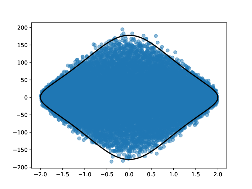
(a) $M=L=100$ and $g=g_{0}=1.25$

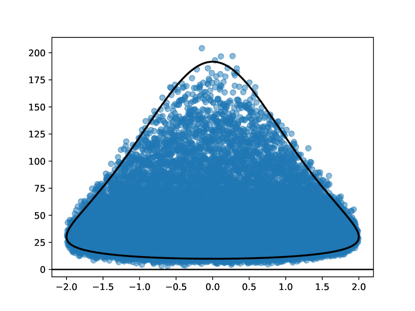
(b) $M=L=100,\,g=1.25$ and $g_{0}=5.05$

Figure 1: Eigenvalues of five $4000\times 4000$ matrices with the solid line indicating equations 15 (top) and 17 (bottom)

In particular, we see that if $p=0$ then the zeros are all in the upper half-plane, separated from the real axis by the gap $\frac{M}{2(g+1)}$. Remembering that for $p=0$ zeroes are mirror images of poles, this result is simply $L=0$ case of fyodorov_systematic_1999 . The gap in the poles distribution is the well-known feature first derived in haak92 and lehmann_chaotic_1995 in the related, but slightly different limit $M=O(N)$. It has profound consequences for underlying dynamics and also has a semiclassic significance, being related to the classic escape timeGaspardRice89a ; GaspardRice89b . Moreover, one can see that all the S-matrix zeros will still be in the same half-plane as long as $|pg-g_{0}|>1+p$ (upper half-plane for $g_{0}-pg>1+p$ and lower for $pg-g_{0}>1+p$). An illustration of such a situation is given in the figure 1(b).

When $|z_{1}-z_{2}|=O(1/N)$, the kernel can be reduced after some algebraic manipulations to the Ginibre-like form:

$$|K(z_{1},z_{2}^{*})| =\widetilde{\rho}(z)e^{-\frac{\pi}{2}\widetilde{\rho}(z)|z_{1}-z_{2}|^{2}},$$ (18)

where $z=\frac{z_{1}+z_{2}}{2}$ and $\widetilde{\rho}(z)$ is from 16. Such a kernel was found in the $L=0$ case when $M\to\infty$ fyodorov_systematic_1999 and is conjectured to be the universal form of the kernel for strongly non-Hermitian matrices fyodorov_random_2003 .

We also record for completeness the general expression for the density of zeros, valid for any $M,L$:

$$\widetilde{\rho}(x,y)=\frac{1}{(g+g_{0})^{M+L-1}}\,\int_{-1}^{1}due^{-2uy}(g+u)^{M}(g_{0}-u)^{L}$$

$$\times \left\{\theta(-y)e^{2g_{0}y}\sum_{n=1}^{L}a_{n}(L,M)\frac{[-2(g+g_{0})y]^{n-1}}{\Gamma(n)}\right.$$

$$\quad\left.+\theta(y)e^{-2gy}\sum_{n=1}^{M}a_{n}(M,L)\frac{[2(g+g_{0})y]^{n-1}}{\Gamma(n)}\right\},$$ (19)

where

$$a_{n}(M,L)=\frac{\Gamma(M+L-n)}{\Gamma(M-n+1)\Gamma(L)}.$$ (20)

The above mean density in $y$ for $x=0$ is compared with RMT simulations in figures 2(a) and 2(b).

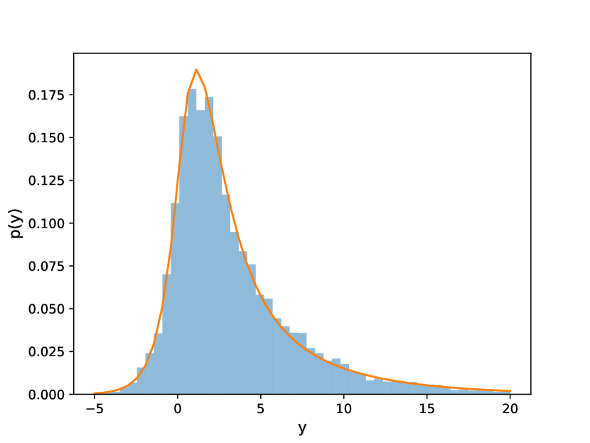
(a) $N=100,\,M=4,\,L=2$

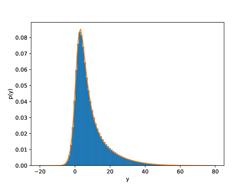
(b) $N=500,\,M=10,\,L=5$

Figure 2: Density of the imaginary parts $\Im z_{n}$ for $\Re z_{n}=0$ compared against II (solid line).

III Statistics of Reflection Time Difference for systems with broken time reversal invariance

In this section we convert the information about $S-$matrix zeroes into information about the two-point connected correlation function of the Reflection Time difference $\delta\mathcal{T}$ defined via (10). In doing this we largely follow the method proposed in FTS98 for the Wigner time delays. We start with recalling that the main microscopic energy scale characterizing (real) eigenvalues of the Hermitian RMT cavity Hamiltonian $H_{0}$ is the associated mean level spacing $\Delta=[N\nu(E)]^{-1}$, and introduce the appropriately rescaled RTD via $\widetilde{\delta\mathcal{T}}=\frac{\Delta}{2\pi}\delta\mathcal{T}$. From the technical point of view it is more natural to consider the associated Fourier transform of the two-point correlation function in question defined as

$$C_{M,L}(t) :=\frac{1}{2\pi}\int d\omega\,e^{i\omega t}\langle\widetilde{\delta\mathcal{T}}\left(E+\frac{\Delta}{2\pi}\omega\right)\widetilde{\delta\mathcal{T}}\left(E-\frac{\Delta}{2\pi}\omega\right)\rangle_{c}.$$ (21)

Defining the so-called empirical density of $S-$matrix zeroes $z_{n}$ in the complex plane $z=\Im z+i\Re z$ as

$$\rho(z)=\frac{1}{N}\sum_{n=1}^{N}\delta^{(2)}(z-z_{n}),$$ (22)

where $\delta^{(2)}(z-z_{n}):=\delta(\Re z-\Re z_{n})\delta(\Im z-\Im z_{n})$, with $\delta(x)$ being the standard Dirac delta-function, we first rewrite (10) as

$$\widetilde{\delta\mathcal{T}}(E)=\frac{\Delta\,N}{2\pi}\int\frac{2\Im z}{(E-\Re z)^{2}+(\Im z)^{2}}\,\rho(z)\,\,d\Re z\,d\Im z,$$ (23)

and then substitute this in (21) and perform the ensemble averaging. In doing this we exploit the relation between covariance functions of empirical densities and the two-point function featuring in (11) for $n=2$, hence the associated kernel (12):

$$\left\langle\rho(z_{1})\rho(z_{2})\right\rangle_{c}=\left\langle\rho(z_{1})\right\rangle\delta(z_{1}-z_{2})-\mathcal{Y}_{2}(z_{1},z_{2}),$$ (24)

where $\mathcal{Y}_{2}(z_{1},z_{2})=|K(z_{1},z_{2}^{*})|^{2}$ is the associated two-point “cluster" function. After rescaling and straightforward manipulations this brings (21) to the form

$$C_{M,L}(t>0)=A(t)-B(t),\quad A(t)=\frac{1}{2}\int dye^{-2\lvert y\rvert t}\widetilde{\rho}(E,y),$$ (25)

and

$$B(t)=\frac{1}{2\pi}\int d\omega dy_{1}dy_{2}\,e^{-it\omega-(\lvert y_{1}\rvert+\lvert y_{2}\rvert)t}$$ (26)

$$\times\mathcal{Y}_{2}(E,\omega,y_{1},y_{2})\,\text{sign}(y_{1}y_{2}),$$

Finally, using the expression 12 for the kernel, we arrive at the following formulas:

$$A(t) =\frac{1}{4}\int_{-1}^{1}du\frac{(g+u)^{M}(g_{0}-u)^{L}}{(g+g_{0})^{M+L}}$$ (27)

$$\quad\quad\times\left[\sum_{n=1}^{M}a_{n}(M,L)\left(\frac{g+g_{0}}{g+t+u}\right)^{n}\right.$$

$$\quad\quad\left.+\sum_{n=1}^{L}a_{n}(L,M)\left(\frac{g+g_{0}}{g_{0}+t-u}\right)^{n}\right],$$

$$B(t)=\frac{\theta(2-t)}{4}\int_{-1}^{1-t}du\frac{(g+u)^{M}(g_{0}-u)^{L}}{(g+g_{0})^{2(M+L)}}(g+t+u)^{M}$$

$$\qquad\times(g_{0}-t-u)^{L}\left[\sum_{n=1}^{M}a_{n}(M,L)\left(\frac{g+g_{0}}{g+t+u}\right)^{n}\right.$$

$$\left.\quad\quad-\sum_{n=1}^{L}a_{n}(L,M)\left(\frac{g+g_{0}}{g_{0}-u}\right)^{n}\right]^{2}.$$ (28)

where $a_{n}(L,M)$ has been defined in (20).

A few remarks are due. First, the limit of no absorption is equivalent to sending $g_{0}\to\infty$. The dominant contribution then obviously comes from the $n=M$ term in the first sum, in both $A(t)$ and $B(t)$. The resulting expression reproduces the well-known correlation function of the Wigner time delay for systems with broken time-reversal invariance: FSS96 ; fyodorov_statistics_1997 :

$$C_{M,0}(t) =\frac{1}{4}\int_{\text{max}(1-t,-1)}^{1}\left(\frac{g+u}{g+t+u}\right)^{M}du,$$ (29)

Note that the above correlation function of Wigner time delays decays as $t^{-M}$ for $t\to\infty$, whereas the corresponding correlation of RTD for any finite absorption $g_{0}<\infty$ decays in the same limit as $t^{-1}$ for any fixed value $M>0,L>0$. This implies that the variance of the RTD which in view of (21) can be found as

$$\left\langle\left[\widetilde{\delta\mathcal{T}}\left(E\right)\right]^{2}\right\rangle_{c}\propto\int_{0}^{\infty}C_{M,L}(t)dt,$$

logarithmically diverges for any finite number of absorbing channels. This feature is strikingly different from the Wigner time delay, whose variance is infinite only for a single-channel scattering, being finite for any $M>1$. The logarithmic divergence of the variance suggests that the distribution of RTD must have the large-tail behaviour $P(\widetilde{\delta\mathcal{T}})\sim\widetilde{\delta\mathcal{T}}^{-3}$. Although we can not prove this conjecture rigorously in generality, it can be strongly supported by a perturbative argument (sketched in the Appendix) valid in the regime of small absorption in a weakly open system with equivalent channels, $\gamma_{a}=\gamma\ll 1,\rho_{a}=\rho\ll 1$, when imaginary parts of the $S-$matrix zeros are much smaller than their separation: $\langle|\Im z_{n}|\rangle\ll\Delta$. Adapting the argument along the lines used in fyodorov_statistics_1997 for Wigner time delays, and further assuming $\rho\gtrsim\gamma$, the probability density for RTD can be shown to have an algebraic decay with universal exponents,

$$P_{\beta}(\widetilde{\delta\mathcal{T}}) \sim\begin{cases}\lvert\widetilde{\delta\mathcal{T}}\rvert^{-3/2},&1\ll\lvert\widetilde{\delta\mathcal{T}}\rvert\ll\gamma^{-1}\\ \lvert\widetilde{\delta\mathcal{T}}\rvert^{-3},&\lvert\widetilde{\delta\mathcal{T}}\rvert\gg\gamma^{-1}\end{cases},$$ (30)

and similarly for negative $\widetilde{\delta\mathcal{T}}$ with $\gamma$ and $\rho$ exchanging their roles. This result is “superuniversal”, that is holding not only for systems with broken symmetry, but for all standard symmetry classes of $H_{0}$ described by values of the Dyson index $\beta=1,2,4$ and for all $M>0,L>0$. We indeed see that the infinite variance is due to the cubic asymptotic decay in the probability density. Note that in the case of Wigner time delay $\tau$ the asymptotic tail of the probability density is rather $\tau^{-\beta M/2-2}$ making the variance finite for $M>2/\beta$. Anticipating that for $\rho=0$ RTD should be indistinguishable from the Wigner time delay, one may consider the parameter range $\rho\ll\gamma$ and find that in that case the decay $\widetilde{\delta\mathcal{T}}^{-\beta M/2-2}$ also happens for RTD in the intermediate asymptotic range $1/\gamma\ll\widetilde{\delta\mathcal{T}}\ll 1/\rho$, whereas the cubic tail takes over only as $\widetilde{\delta\mathcal{T}}\gg 1/\rho$, reconciling the two types of behaviour.

One also can be interested in the short-time behaviour of the RTD correlation function. Considering for simplicity the simplest case $M=L=1$, we obtain in this limit:

$$C_{1,1}(t\ll 1) =\frac{1}{2}\left[1-\frac{4+3(g-g_{0})^{2}}{3(g+g_{0})^{2}}\right]$$

$$+\frac{(g-g_{0})^{2}-4(g+g_{0}-1)}{4(g+g_{0})^{2}}t+O(t^{2}).$$ (31)

The first order term vanishes when $g^{\pm}_{0}=g+2\pm 2\sqrt{2g}$ and vice versa. For $1<g<3+2\sqrt{2}$, the second solution $g^{-}_{0}=g+2-2\sqrt{2g}<1$ is not valid since $g,g_{0}>1$ by definition. Thus, the correlator switches from an increasing to a decreasing function of time as $g_{0}$ passes through $g_{0}^{+}$. Reverting to the frequency domain, we find that in this case correlator decays as $\omega^{-4}$, whereas the correlator of the Wigner time delay always decays as $\omega^{-2}$ since $\dot{C}_{M,0}(0)=1/4$.

Another curious observation is that due to appearance of the factor $\text{sign}(y_{1}y_{2})$ in the integrand of (32), the term $B(t)$ identically vanishes when $\mathcal{Y}_{2}$ is even in $y_{1}$ and $y_{2}$ separately, in which case $C(t)$ only depends on the mean global density of complex eigenvalues rather than on the two-point correlation function. For equivalent channels, a necessary condition for this to happen is $M=L$ and $g=g_{0}$.

To compare with numerical simulations, we find that instead of directly computing 21, it is more practical to consider instead the Fourier transform of the RTD weighted by a Gaussian:

$$F(t,W) :=\int\frac{dE}{\sqrt{2\pi W}}\widetilde{\delta\mathcal{T}}(E)e^{iEt-\frac{E^{2}}{2W}}$$ (32)

$$=\sqrt{\frac{\pi}{2W}}e^{-\frac{Wt^{2}}{2}}\sum_{n=1}^{N}\text{sign}(\Im z_{n})$$

$$\times\left[\text{erfcx}\left(\frac{|\Im z_{n}|+Wt+i\Re z_{n}}{\sqrt{2W}}\right)\right.$$

$$+\left.\text{erfcx}\left(\frac{|\Im z_{n}|-Wt-i\Re z_{n}}{\sqrt{2W}}\right)\right],$$ (33)

where $\text{erfcx}(z)=e^{z^{2}}\text{erfc}(z)$ and $\text{erfc}(z)=\frac{2}{\sqrt{\pi}}\int_{z}^{\infty}e^{-x^{2}}dx$ is the complementary error function. If we take $\frac{1}{N}\ll\sqrt{W}\ll 1$, then we find the approximate relation:

$$\frac{\Delta}{4\pi}\sqrt{\frac{W}{\pi}}\langle|F\left(\frac{\pi t}{\Delta};W\right)|^{2}\rangle_{c} \approx C_{M,L}(t).$$ (34)

The advantage of this approach is that the ensemble average of $F(t;W)$ converges faster than that of the RTD. Figures 3(a) and 3(b) compare the correlator obtained in this way from RMT simulations ($N=300$) with the prediction for $M=1$ and $L=0,1$.

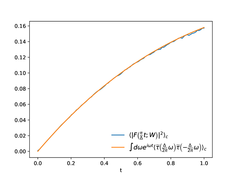
(a) $M=1,L=0,g=1.25$

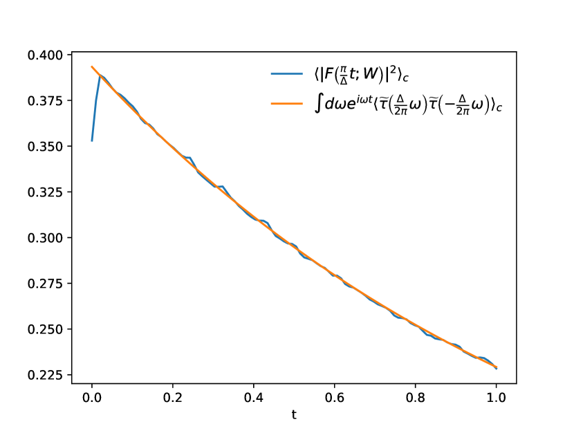
(b) $M=1,L=1,g=g_{0}=1.25$

Figure 3: $C_{M,L}(t)$ of 21 compared with simulations of $300\times 300$ random matrices, using 34 as an estimator. The small time discrepancy in the second figure appears to be a finite-size effect which occurs over a smaller window in time as the dimension of the matrices increases.

IV On extracting S-matrix zeros from scattering data

Let us now discuss a possibility of determining the positions of the zeros of a subunitary scattering matrix from an experiment, real or numerical. One may imagine two possibilities: either one has access to the total unitary $\mathcal{S}$ matrix, or only to its subunitary observable/scattering block $S(E)$. Indeed, one may consider constructing a CPA in the form of a three port microwave network where one port plays the role of the attenuator providing absorption. In such a setup, if one disregards imperfections in the setup, the output in all three ports is directly accessible, hence the total $\mathcal{S}$ matrix.

In the usual case of $S-$matrix poles, one of the most well-established methods for determining their positions in the lower half-plane is the “harmonic inversion” wiersig_fractal_2008 , which estimates the poles by solving a set of non-linear equations. In a nutshell, one estimates a signal represented in the time domain as a sum of decaying exponentials evaluated at times $t=n\tau$, where $\tau$ is the sample rate, by relying on the Padé approximation:

$$c_{n} :=\sum_{k=1}^{N}d_{k}e^{-iz_{k}n\tau},$$ (35)

$$f(z) :=\sum_{n=0}^{\infty}c_{n}z^{-n}=\sum_{k=1}^{N}\frac{d_{k}z_{k}}{z-z_{k}}$$ (36)

$$=\frac{P_{K}(z)}{Q_{K}(z)},$$ (37)

where $P_{K}/Q_{K}$ is the order $(K,K)$ Padé approximant to $f(z)$. The zeros $z_{k}$ are the poles of $Q(z)$ and the amplitudes $d_{k}$ are the ratio of the residues and the poles. The integer $K$ is chosen as an upper bound to the number of true zeros $N$, leading to $N-K$ spurious zeros which must be discarded. In general, it is common to introduce a cut-off and discard zeros for which the magnitude of the residue falls below the cut-off. The procedure for $S-$ matrix poles outlined in kuhl_resonance_2008 used both a cut-off and discarding those poles whose imaginary parts were smaller than the energy spacing (distance between energy samples), as well as with real parts near the boundary of the sampling window.

Harmonic inversion can be performed directly on the $S-$matrix elements or, alternatively, on the Wigner time delay. When estimating zeros, the signal to be considered is given by the inverse of the determinant:

$$\frac{1}{\det S(E)} =\prod_{n=1}^{N}\frac{E-E_{n}+i\Gamma_{n}/2}{E-\Re z_{n}-i\Im z_{n}}.$$ (38)

Alternatively, when the whole unitary $\mathcal{S}$ can be measured, one can use the expression 10 for the RTD. Assuming additionally a weak uniform absorption $\epsilon\ll 1$ inside the scattering domain, the RTD can be alternatively computed from the unitary deficit of the determinant ratio, see fyodorov_reflection_2019 for a discussion:

$$\delta\mathcal{T}(E) =-\frac{1}{\epsilon}\Re\log\frac{\det S(E+i\epsilon)}{\det S^{\prime}(E+i\epsilon)}+O(\epsilon^{2}).$$ (39)

The advantage of using the RTD for extracting positions of complex zeroes is that the Lorentzians in the sum are all normalised to unity, providing us with a way to distinguish true and spurious zeros by looking at the corresponding residues. The residues in 38 involve instead a product over the remaining zeros and poles which can take arbitrary values. It is not a priori clear how to choose an appropriate cut-off, particularly when the zeros/poles appear as Lorentzians with varying amplitudes. We compare the performance of both methods for extracting the zeros by simulating $H_{0}$ from the GUE; parameters affecting the accuracy of the estimates are the number of samples $nE$ of $S(E)$ and the strength of the uniform absorption $\epsilon$. Since the first step of the harmonic inversion procedure is to take the Fourier transform, when using 38 we perform a second transform on the complex conjugate so that the zeros in both half-planes are accounted for. The detection of spurious zeros differs between the two methods. In the first method, we follow kuhl_resonance_2008 in using a cut-off and removing zeros near the boundaries. The cut-off has been chosen as 1, the value accounting well for most of the spurious zeros. In the second method, the zeros occur in complex conjugate pairs whose residues (after normalising by the energy spacing) should add up to 1. We therefore grouped the zeros into conjugate pairs and removed those whose residues were significantly different from 1. This allowed us to bypass the need for the removal of zeros near the boundaries. Figure 5 shows the true zeros plotted against those estimated from 38 and 39, for various parameter configurations. In figures 4(a) and 5(a), there are what appear to be spurious zeros (isolated green crosses) among those estimated by the second method. These arise because of the appearance of two complex conjugate pairs for the same zero; in general we observe that as the strength of the uniform absorption $\epsilon$ increases, an increasing number of zeros are associated with two or more complex conjugate pairs. This is why these do not appear in figures 4(b) and 5(b), where $\epsilon=10^{-6}$. One could attempt to group all pairs in order to bring the sum of resiudes closer to one, or simply discard all but one pair. Note also that in all four figures there are zeros near the boundaries which are discarded in the first method but included in the second.

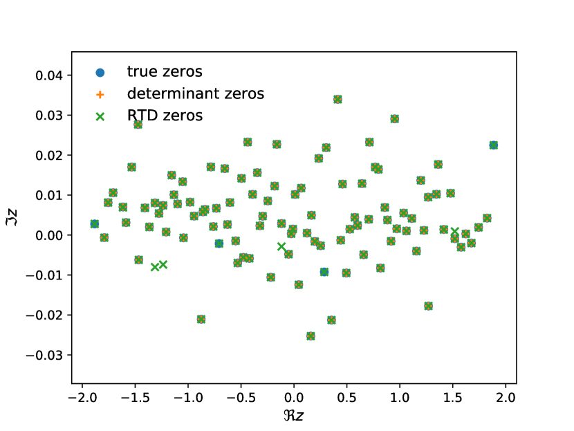
(a) $\gamma=0.5,\rho=0.5,nE=800,\epsilon=10^{-5}$

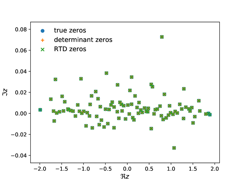
(b) $\gamma=0.5,\rho=0.5,nE=800,\epsilon=10^{-6}$

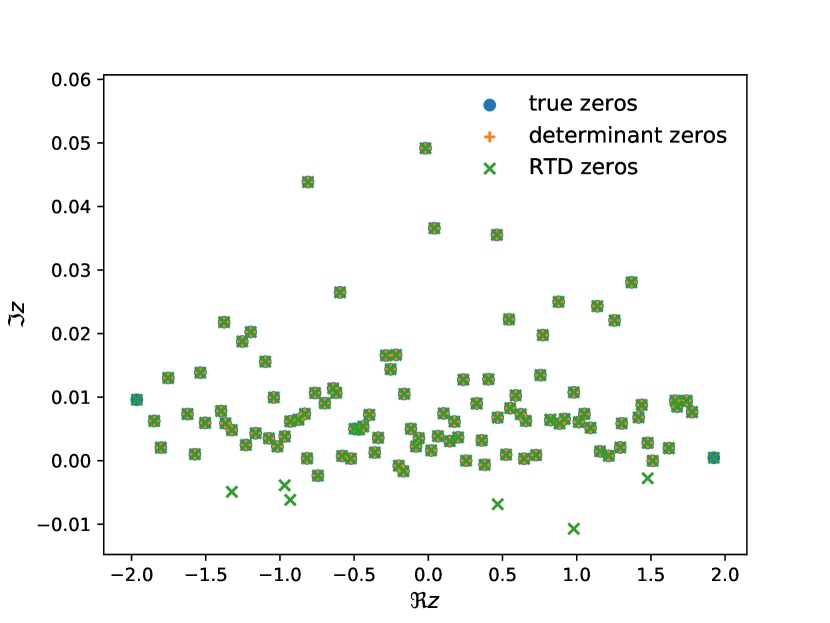
(a) $\gamma=0.5,\rho=0.1,nE=800,\epsilon=10^{-5}$

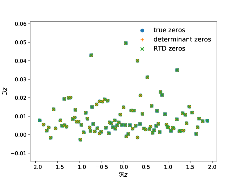
(b) $\gamma=0.5,\rho=0.1,nE=800,\epsilon=10^{-6}$

Figure 5: Estimated zeros using 38 (orange plus signs) and using 39 (green crosses) compared to true zeros (blue circles). In all cases, $N=100,M=2,L=1$.

V Discussion and open problems.

In conclusion, we have studied the statistics of the zeros of the subunitary $S$ matrix for a RMT-based model of scattering in chaotic cavities with localized absorption and broken time-reversal symmetry. The $n$-point correlation functions of the zeroes in the complex plane for a system with a finite number of scattering and absorbing channels ($M$ and $L$, respectively) can be calculated by extending the method used in fyodorov_systematic_1999 for characterizing the $S-$matrix poles (formally equivalent to the $L=0$ case). The resulting kernel, in the limit of strong non-Hermiticity with at least one of the parameters $M$ and/or $L$ going to infinity, takes the form of a generalised Ginibre kernel, expected to be universal in this regime fyodorov_random_2003 . For finite $M<\infty$ and $L<\infty$, the kernel was used to obtain the Fourier transform of the correlation function $C_{M,L}(t)$ of the RTD, which has been shown to decay as $C_{M,L}(t)\sim t^{-1}$ at large times for any $L>0$. This is in sharp contrast with the case $L=0$ (formally equivalent to replacing RTD with the Wigner time delay), where a similar tail is known to be $M$-dependendent: $\sim t^{-M}$. In particular, this implies that the variance of the RTD is infinite regardless of the value of $M$ or $L$. We interpret this divergence as an evidence for the existence of a far tail $P(\widetilde{\delta\mathcal{T}})\sim\delta\mathcal{T}(E)^{-3}$ in the RTD probability density, and verify this in the regime of weakly open and weakly absorbing system. We expect such a tail to be a superuniversal feature of the RTD distribition valid for all symmetry classes.

The short time behaviour of the RTD correlation function is again markedly different for $L=0$ and $L>0$: $C_{M,0}(t)\sim\frac{1}{4}t$ in the former case and $C_{M,L}(t)\sim C_{M,L}(0)+\dot{C}_{M,L}(0)t$ in the latter, with $C_{M,L}(0)\neq 0$ and the coefficient $\dot{C}_{M,L}(0)$ depending on $g$ and $g_{0}$ in such a way that it changes from a positive value through zero to negative values as $g_{0}$ is reduced from infinity towards unity. This implies that there must exist a particular value of absorption parameter $g_{0}$ (depending on $g$) such that the large frequency asymptotic of the Fourier-transformed correlation function decays as $\omega^{-4}$ instead of the typical decay $\omega^{-2}$.

We have also examined two methods for extracting the positions of $S-$matrix zeros from experimental scattering data by harmonic inversion of either the inverse determinant of $S$ or from the RTD. The first method is applicable when only the scattering part of $S$ is available, while for the second method the total $\mathcal{S}$ matrix must be accessible. The advantage of the second method is that we know in advance the residue of each zero, which allows us to distinguish more easily between true and spurious zeros. In the recent papers demonstrating the construction of a disordered CPA pichler_random_2019 ; chen_perfect_2020 the $S$ matrix was measured at regular intervals in an energy window, but rather than determine the zeros, each $S$ matrix was diagonalised and the eigenvalue closest to zero selected as a candidate for the CPA state. Using harmonic inversion one can instead directly estimate the zeros themselves.

Finally, let us mention that all non-perturbative treatment in our paper has been restricted to systems with broken time-reversal invariance. Actually, the mean density of complex eigenvalues $z_{n}$ for chaotic systems with preserved time-reversal invariance, with $H_{0}$ being taken from the Gaussian Orthogonal Ensemble, can be deduced for $L>0$ from known $L=0$ results by an ad hoc analytic contunuation, see fyodorov_distribution_2017 . However its systematic controllable derivation, not speaking about deducing the form of the two-point (and higher) correlation functions, remains an outstanding and challenging problem. This currently prevents us from any non-perturbative insights into statistics of the Reflection Time Difference (apart from its expected superuniversal cubic tail in the probability density) for this important case.

Appendix

Derivation of the correlation function of $S-$matrix zeros.

We give a brief sketch of the derivation of the exprression 12 for the $n$-point correlation function. Since the derivation follows mainly the steps of fyodorov_systematic_1999 (explained in more detail in fyodorov_random_2003 ), we omit the detail and point out only the necessary modification. The object of study is the spectrum of the perturbed GUE matrix $J=H+i\Gamma$, where $\Gamma=\text{diag}(\gamma_{1},...,\gamma_{M+L},0,...,0)$ is a rank $M+L$ matrix where $\gamma_{1}\geq\cdots\geq\gamma_{M}>0>\gamma_{M+1}\geq\cdots\gamma_{M+L}$. It is the fact that the matrix $\Gamma$ has eigenvalues of both signs which makes a difference from fyodorov_systematic_1999 and should be properly accounted for. The joint probability density for the matrix $J$ induced by $H$ is:

$$P(J)dJ \propto e^{-\frac{N}{2}\text{tr}\left(\frac{J+J^{\dagger}}{2}\right)^{2}}\delta\left(\frac{J-J^{\dagger}}{2i}-\Gamma\right),$$ (40)

where $\delta(A)=\prod_{i,j}\delta(A_{ij})$. Making use of the Schur decomposition $J=U(Z+R)U^{\dagger}$, the integral over the upper triangular matrix $R$ can be performed with the delta function in the off-diagonal elements. The remaining delta functions in the diagonal elements are represented by a Fourier integral over a diagonal matrix $K$, leaving a Harish-Chandra/Itzykson/Zuber (HCIZ) integral with $K$ and $\Gamma$. Since $\Gamma$ is not of full rank, the limit of $N-M-L$ eigenvalues going to zero is calculated by repeated application of l’Hôpital’s rule to the original HCIZ formula. The result is the following expression for the density of eigenvalues $Z$:

$$P(Z)\propto\frac{\lvert\Delta(Z)\rvert^{2}}{\text{det}^{N-M-L}(\gamma)\Delta(\gamma)}e^{-\frac{N}{2}\Re\text{tr}Z^{2}-\frac{N}{2}\text{tr}\gamma^{2}}$$ (41)

$$\times\int\frac{dK}{(2\pi)^{N}}\frac{e^{i\text{tr}K\Im Z}}{\Delta(K)}\,{\cal D}(K)$$

where we denoted $\gamma=\text{diag}(\gamma_{1},...,\gamma_{M+L})$ and introduced

$${\cal D}(K):=$$ (42)

$$\text{det}\begin{vmatrix}e^{-ik_{1}\gamma_{1}}&\cdots&e^{-ik_{1}\gamma_{M+L}}&(-ik_{1})^{N-M-L-1}&\cdots&1\\ \vdots&\ddots&\vdots&\vdots&\ddots&\vdots\\ e^{-ik_{N}\gamma_{1}}&\cdots&e^{-ik_{N}\gamma_{M+L}}&(-ik_{N})^{N-M-L-1}&\cdots&1\end{vmatrix}.$$

The difference now from the original derivation is that the terms $e^{-ik_{j}\gamma_{c}}$ are represented by the integral:

$$e^{-ik_{j}\gamma_{c}} =\frac{1}{2\pi i}\int_{\mathcal{L}_{c}}\frac{e^{-ik_{j}\lambda_{c}}}{\lambda_{c}-k_{j}}d\lambda_{c},$$ (43)

where $\mathcal{L}_{c}=\text{sign}(\gamma_{c})(-\mathbb{R}+i0)$. After taking the $\lambda$ integrals outside the determinant and using the following identity:

$$\det\begin{vmatrix}\frac{1}{\lambda_{1}-k_{1}}&\cdots&\frac{1}{\lambda_{\mathcal{M}}-k_{1}}&(-ik_{1})^{N-\mathcal{M}-1}&\cdots&1\\ \vdots&\ddots&\vdots&\ddots&\vdots\\ \frac{1}{\lambda_{1}-k_{N}}&\cdots&\frac{1}{\lambda_{\mathcal{M}}-k_{N}}&(-ik_{N})^{N-\mathcal{M}-1}&\cdots&1\end{vmatrix}$$

$$\propto\frac{\Delta(\Lambda)\Delta(K)}{\prod_{j=1}^{\mathcal{M}}\prod_{i=1}^{N}(\lambda_{j}-k_{i})},$$ (44)

which follows by elementary row and column operations, the final expression for the density $P(Z)$ is:

$$P(Z) \propto\frac{1}{\det^{N-\mathcal{M}}(\gamma)\Delta(\gamma)}\lvert\Delta(Z)\rvert^{2}e^{-\frac{N}{2}\text{Re}\text{tr}Z^{2}-\frac{N}{2}\text{tr}\gamma^{2}}$$

$$\quad\times\int_{\mathcal{L}_{1}}\cdots\int_{\mathcal{L}_{\mathcal{M}}}d\Lambda\Delta(\Lambda)e^{-i\sum_{j=1}^{\mathcal{M}}\gamma_{j}\lambda_{j}}$$

$$\times\prod_{i=1}^{N}\sum_{j=1}^{\mathcal{M}}\frac{e^{i\lambda_{j}\text{Im}z_{i}}}{\prod_{l\neq j}(\lambda_{l}-\lambda_{j})}\theta(\text{Im}\lambda_{j}\text{Im}z_{i}),$$ (45)

From this point onwards the derivation follows exactly along the lines of fyodorov_random_2003 , where in the appendix of that paper the $n$-point correlation function is related to the average of a product of characteristic polynomials which is subsequently evaluated by integrating over anti-commuting variables.

Distribution of RTD in the regime of weak coupling and absorption.

In this regime the imaginary part of the zeroes is much smaller than the typical separation between the real parts, and, moreover, imaginary parts of neighbouring zeroes are independent to the leading order. Then the dominant contribution to RTD at a given real energy $E$ can be estimated by a heuristic argument fyodorov_statistics_1997 that takes into account only the zero whose real part is the closest to the energy value $E$ in the sum of Lorentzians 10. Attributing the index $n$ to this particular zero and defining $u_{n}=\frac{\beta\pi}{\Delta}(E-\Re z_{n})$ and $y_{n}=\frac{\beta\pi}{\Delta}\Im z_{n}$, we have

$$\widetilde{\delta\mathcal{T}}(E) \simeq\frac{2y_{n}}{u_{n}^{2}+y_{n}^{2}}.$$ (46)

The real and imaginary parts of $z_{n}$ are independent in the weak coupling regime, with the latter having the density:

$$P^{\beta}_{Y}(y) =\int\frac{dk}{2\pi}\frac{e^{iky}}{\prod_{a=1}^{M}(1+2ik\gamma_{a})^{\beta/2}\prod_{b=1}^{L}(1-2ik\rho_{b})^{\beta/2}}.$$ (47)

We also assume that $u_{n}$ is uniformly distributed in $[-\beta\pi,\beta\pi]$. The result of these approximations is the following estimate for the density of $\widetilde{\delta\mathcal{T}}\equiv\tau$:

$$P_{\widetilde{\delta\mathcal{T}}}^{\beta}(\tau) =\int dyP_{\beta}(y)\int_{-\beta\pi}^{\beta\pi}du\delta\left(\tau-\frac{2y}{u^{2}+y^{2}}\right)$$ (48)

$$\simeq\frac{2}{\tau^{3}}\int_{0}^{\min(1,\frac{\beta^{2}\pi^{2}\tau^{2}}{4})}\sqrt{\frac{y}{1-y}}\left[\theta(\tau)P^{\beta}_{Y}\left(\frac{2y}{\tau}\right)\right.$$ (49)

$$\left.+\theta(-\tau)P_{Y}^{\beta}\left(-\frac{2y}{\tau}\right)\right]dy.$$

Focusing on positive $\widetilde{\delta\mathcal{T}}$ and equivalent channels $\gamma_{a}=\gamma\ll 1,\rho_{b}=\rho\ll 1$, let us first assume that $\rho\gtrsim\gamma$. Then we can identify two regimes for $\tau>2/(\beta\pi)$: i) $\tau\gamma\ll 1$ and ii) $\tau\gamma\gg 1$. In the first regime, the dominant term in $P^{\beta}_{Y}(2y/(M\tau))$ is $y^{\beta M/2-1}e^{-\frac{y}{\tau\gamma}}$:

$$P^{\beta}_{\widetilde{\delta\mathcal{T}}}(\tau) \simeq\frac{\gamma^{\beta L/2-1}}{\tau^{3}\Gamma(\beta M/2)(\gamma+\rho)^{\beta L/2}}$$ (50)

$$\times\int_{0}^{\infty}\sqrt{y}\left(\frac{y}{\tau\gamma}\right)^{\beta M/2-1}e^{-\frac{y}{\tau\gamma}}dy$$

$$=\frac{\gamma^{\beta(L+1)/2}}{(\gamma+\rho)^{\beta L/2}}\tau^{-3/2},$$ (51)

where we have set the upper limit of integration to infinity and taken $1-y\simeq 1$, both justified by the exponential damping. In the second regime, the dominant term is now just $e^{-\frac{y}{\tau\gamma}}$, which is approximately unity:

$$P^{\beta}_{\widetilde{\delta\mathcal{T}}}(\tau) \simeq\frac{\Gamma(\beta(M+L)/2-1)}{\Gamma(\beta M/2)\Gamma(\beta L/2)}\frac{1}{\tau^{3}\gamma^{\beta M/2}\rho^{\beta L/2}}$$ (52)

$$\times\left(\frac{\gamma\rho}{\gamma+\rho}\right)^{\beta(M+L)/2-1}\int_{0}^{1}\sqrt{\frac{y}{1-y}}$$

$$=\frac{\pi\Gamma(\beta(M+L)/2-1)}{2\Gamma(\beta M/2)\Gamma(\beta L/2)}$$ (53)

$$\times\frac{1}{\gamma^{\beta M/2}\rho^{\beta L/2}}\left(\frac{\gamma\rho}{\gamma+\rho}\right)^{\beta(M+L)/2-1}\tau^{-3}.$$

Thus we see that $P^{\beta}_{\widetilde{\delta\mathcal{T}}}(\tau)$ behaves as a power law with universal exponents, summarized in (30).

If one however assumes $\rho\ll\gamma$ and repeats the analysis above, one finds that the regime $\tau\gg 1/\gamma$ should be further subdivided into two new regimes: $1/\gamma\tau\ll 1/\rho$ and $\tau\gg 1/\rho$. Only in the latter case one reproduces the superuniversal asymptotics $P^{\beta}_{\widetilde{\delta\mathcal{T}}}(\tau)\simeq\tau^{-3}$ whereas in the former the asymptotic is changed to $P^{\beta}_{\widetilde{\delta\mathcal{T}}}(\tau)\simeq\tau^{-(2+\beta M/2)}$. This type of tail behaviour is precisely one which is typical for the Wigner time delays, to which the RTD formally reduces as $\rho\to 0$.

The same arguments can be made for negative $\widetilde{\delta\mathcal{T}}$ by exchanging the role of $\gamma$ with that of $\rho$.

References

- (1) U. Kuhl, O. Legrand, and F. Mortessagne. Microwave experiments using open chaotic cavities in the realm of the effective Hamiltonian formalism. Fortschr. Phys., 61, 414–419 (2013)
- (2) G. Gradoni, J.-H. Yeh, B. Xiao, T.-M. Antonsen , S.-M. Anlage, and E. Ott. Predicting the statistics of wave transport through chaotic cavities by the Random Coupling Model: a review and recent progress. Wave Motion, 51, 606–621 (2014)
- (3) B. Dietz and A. Richter. Quantum and wave dynamical chaos in superconducting microwave billiards. Chaos, 25, 097601 (2015)
- (4) H. Cao and J. Wiersig. Dielectric microcavities: Model systems for wave chaos and non-Hermitian physics." Rev. Mod. Phys., 87, 61–111 (2015)
- (5) G. E. Mitchell, A. Richter, and H.A. Weidenmueller. Random Matrices and Chaos in Nuclear Physics: Nuclear Reactions. Rev. Mod. Phys.82 (4), 2845–2901 (2010) [doi: 10.1103/RevModPhys.82.2845]
- (6) Y.V. Fyodorov and D.V. Savin. Resonance Scattering of Waves in Chaotic Systems in: The Oxford Handbook of Random Matrix Theory, ed. by G. Akemann, J. Baik and P. Di Francesco (Oxford University Press, 2011)
- (7) H. Schomerus. Random matrix approaches to open quantum systems. Les Houches summer school on ”Stochastic Processes and Random Matrices”, 2015, Ed. G. Schehr et al. (Oxford University Press, 2017)
- (8) R. Schaefer, T. Gorin, T.H. Seligman, and H.-J. Stoeckmann. Correlation Functions of Scattering Matrix Elements in Microwave Cavities with Strong Absorption. J. Phys. A: Math. Gen. 36, no.12, 3289–3302 (2003)[doi: 10.1088/0305-4470/36/12/325]
- (9) R.A. Mendez-Sanchez, U. Kuhl, M. Barth, C.V. Lewenkopf, and H.-J. Stöckmann. Distribution of reflection coefficients in absorbing chaotic microwave cavities. Phys. Rev. Lett. 91, 174102 (2003).
- (10) S. Hemmady, X. Zheng, E. Ott, T.M. Antonsen, S.M. Anlage. Universal impedance fluctuations in wave chaotic systems. Phys. Rev. Lett. 94, 014102 (2005).
- (11) S. Hemmady, X. Zheng, J. Hart, T. M. Antonsen, E. Ott, and S. M. Anlage, Universal properties of two-port scattering, impedance, and admittance matrices of wave-chaotic systems. Phys. Rev. E 74, 036213 (2006)
- (12) X. Zheng, S. Hemmady, T. M. Antonsen, Jr., S. M. Anlage, and E. Ott. Characterization of fluctuations of impedance and scattering matrices in wave chaotic scattering. Phys. Rev. E 73, 046208 (2006).
- (13) O. Hul, O. Tymoshchuk, S. Bauch, P.M. Koch, and L. Sirko. Experimental investigation of Wigner’s reaction matrix for irregular graphs with absorption. J. Phys. A 38, 10489 (2005).
- (14) M. Lawniczak, O. Hul, S. Bauch, P. Seba, and L. Sirko. Experimental and numerical investigation of the reflection coefficient and the distributions of Wigner’s reaction matrix for irregular graphs with absorption. Phys. Rev. E 77, 056210 (2008).
- (15) M. Lawniczak, S. Bauch, O. Hul, and L. Sirko. Experimental investigation of the enhancement factor for microwave irregular networks with preserved and broken time reversal symmetry in the presence of absorption. Phys. Rev. E 81, 046204 (2010).
- (16) P.W. Brouwer and C.W.J. Beenakker. Voltage-Probe and Imaginary Potential Models for Dephasing in a Chaotic Quantum Dot. Phys. Rev. B 55 no.7, 4695–4702 (1997) [doi: 10.1103/PhysRevB.55.4695]
- (17) C.W.J. Beenakker, P.W.Brouwer, Physica E 9, 463 (2001)
- (18) Y.V. Fyodorov. Induced vs. Spontaneous breakdown of S-matrix unitarity: probability of no return in quantum chaotic and disordered systems. JETP Letters 78, 250–254 (2003).
- (19) Y.V. Fyodorov, D.V. Savin. Statistics of impedance, local density of states, and reflection in quantum chaotic systems with absorption JETP Letters 80 (12), 725–729 (2004)
- (20) D.V. Savin, H.J. Sommers, Y.V. Fyodorov. Universal statistics of the local Green’s function in wave chaotic systems with absorption JETP Letters 82 (8), 544–548 (2005)
- (21) Y. V. Fyodorov, D. V. Savin and H.-J. Sommers. Scattering, reflection and impedance of waves in chaotic and disordered systems with absorption. J. Phys. A: Math. Gen. 38, Issue 49, 10731–10760 (2005)
- (22) I. Rozhkov, Y.V. Fyodorov and R.L. Weaver. Statistics of transmitted power in multichannel dissipative ergodic structures. Phys. Rev. E 68, 016204 (2003)
- (23) I. Rozhkov, Y.V. Fyodorov and R.L. Weaver. Variance of transmitted power in multichannel dissipative ergodic structure invariant under time reversal. Phys. Rev. E 69, 036206 (2004)
- (24) S. B. Fedeli and Y.V. Fyodorov. Statistics of off-diagonal entries of Wigner matrix for chaotic wave systems with absorption. J. Phys. A: Math. Theor. 53, no.16, 165701 [ https://doi.org/10.1088/1751-8121/ab73ab]
- (25) Y. D. Chong, Li Ge, Hui Cao and A.D. Stone. Coherent Perfect Absorbers: Time-Reversed Lasers. Phys. Rev. Lett 105(5), 053901 (2010) [doi: 10.1103/PhysRevLett.105.053901]
- (26) K. Pichler, M. Kühmayer, J. Böhm, A. Brandstötter, P. Ambichl, U. Kuhl, and S. Rotter. Random Anti-Lasing through Coherent Perfect Absorption in a Disordered Medium. Nature 567 No. 7748, 351 (2019) [doi:10.1038/s41586-019-0971-3]
- (27) L. Chen, T. Kottos, S.M. Anlage. Perfect Absorption in Complex Scattering Systems with or without Hidden Symmetries. arXiv:2001.00956
- (28) H. Li, S. Suwunnarat, R. Fleischmann, H. Schanz, and T. Kottos. Random Matrix Theory Approach to Chaotic Coherent Perfect Absorbers. Phys. Rev. Lett. 118 No. 4, 044101 (2017) [doi:10.1103/PhysRevLett.118.044101]
- (29) Y.V. Fyodorov, S. Suwunnarat, T. Kottos. Distribution of zeros of the S-matrix of chaotic cavities with localized losses and coherent perfect absorption: non-perturbative results. J. Phys. A: Math. Theor. 50, Issue 30, 30LT01 (2017) [doi:10.1088/1751-8121/aa793a]
- (30) V.V. Sokolov and V.G. Zelevinsky. Dynamics and statistics of unstable quantum states. Nucl. Phys. A 504, Issue 3, 562–588(1989)
- (31) F. Haake, F. Izrailev, N. Lehmann, D. Saher , and H.-J. Sommers. Statistics of complex levels of random matrices for decaying systems. Z. Phys. B, 88, 359–370 (1992)
- (32) Y. V. Fyodorov and H.-J. Sommers. Statistics of S-matrix poles in few-channel chaotic scattering: Crossover from isolated to overlapping resonances. JETP Lett., 63 1026–1030 (1996).
- (33) Y. V. Fyodorov and H.-J. Sommers. Statistics of resonance poles, phase shifts and time delays in quantum chaotic scattering: Random matrix approach for systems with broken time-reversal invariance. J. Math. Phys. 38, Issue 4, 1918–1981 (1997) [doi:10.1063/1.531919]
- (34) Y. V. Fyodorov, B. A. Khoruzhenko. Systematic Analytical Approach to Correlation Functions of Resonances in Quantum Chaotic Scattering. Phys. Rev. Lett., 83, 65 –68 (1999)
- (35) H.-J. Sommers, Y. V. Fyodorov, and M. Titov. S-matrix poles for chaotic quantum systems as eigenvalues of complex symmetric random matrices: from isolated to overlapping resonances. J. Phys. A: Math. Gen., 32, L77 (1999)
- (36) R. A. Janik, W. Noerenberg, M. A. Nowak, G. Papp, I. Zahed. Correlations of Eigenvectors for Non-Hermitian Random-Matrix Models. , Phys. Rev. E 60, 2699 (1999)
- (37) H. Schomerus, K.M. Frahm, M. Patra, C.W.J. Beenakker. Quantum limit of the laser line width in chaotic cavities and statistics of residues of scattering matrix poles. Physica A, 278, 469–496 (2000)
- (38) Y.V. Fyodorov and B. Mehlig. Statistics of resonances and nonorthogonal eigenfunctions in a model for single-channel chaotic scattering. Phys. Rev. E, 66, 045202(R) (2002)
- (39) Yan V. Fyodorov and H.-J. Sommers. Random Matrices Close to Hermitian or Unitary: Overview of Methods and Results. J. Phys. A: Math. Gen. 36, no.12, 3303–3347 (2003) [doi: 10.1088/0305-4470/36/12/326]
- (40) G. L. Celardo, N. Auerbach, F. M. Izrailev, and V. G. Zelevinsky. Distribution of Resonance Widths and Dynamics of Continuum Coupling. Phys. Rev. Lett. 106, 042501 (2011)
- (41) Y.V. Fyodorov and D.V. Savin. Statistics of resonance width shifts as a signature of eigenfunction nonorthogonality. Phys. Rev. Lett. 108, 184101 (2012)
- (42) Y. V. Fyodorov and D.V. Savin. Resonance width distribution in RMT: Weak-coupling regime beyond Porter-Thomas. EPL, 110, 40006, (2015)
- (43) U. Kuhl, R. Höhmann, J Main, and H.-J. Stöckmann. Resonance Widths in Open Microwave Cavities Studied by Harmonic Inversion. Phys. Rev. Lett. 100, 254201 (2008) [doi: 10.1103/PhysRevLett.100.254101]
- (44) J. Wiersig and J. Main. Fractal Weyl Law for Chaotic Microcavities: Fresnel’s Laws Imply Multifractal Scattering. Phys. Rev. E 77 No.3, 036205 (2008) [doi: 10.1103/PhysRevE.77.036205]
- (45) A. Di Falco, T.-F. Krauss, and A. Fratalocchi. Lifetime statistics of quantum chaos studied by a multiscale analysis. Appl. Phys. Lett., 100, 184101 (2012)
- (46) S. Barkhofen, T. Weich, A. Potzuweit, H.-J. Stöckmann, U. Kuhl , M. Zworski. Experimental observation of the spectral gap in microwave n-disk systems. Phys. Rev. Lett., 110, 164102 (2013)
- (47) C. Liu, A. Di Falco, A. Fratalocchi. Dicke Phase Transition with Multiple Superradiant States in Quantum Chaotic Resonators. Phys. Rev. X, 4, 021048 (2014)
- (48) J.-B. Gros, U. Kuhl, O. Legrand, F. Mortessagne, E. Richalot, and D. V. Savin. Experimental width shift distribution: a test of nonorthogonality for local and global perturbations. Phys. Rev. Lett., 113 224101 (2014)
- (49) L. Wang, D. Lippolis, Z.-Y. Li, X.-F. Jiang, Q. Gong, and Y.-F. Xiao. Statistics of Chaotic Resonances in an Optical Microcavity. Phys. Rev. E 93, 040201(R) (2016)
- (50) M. Davy and A. Z. Genack. Selectively exciting quasi-normal modes in open disordered systems. Nature Commun. 9, Article number: 4714 (2018)
- (51) M. Davy and A. Z. Genack. Probing nonorthogonality of eigenfunctions and its impact on transport through open systems. Physical Review Research1, 033026 (2019)
- (52) E.P. Wigner, Lower limit for the energy derivative of the scattering phase shift. Phys. Rev. 98 (1) 145–-147 (1955)
- (53) F. T. Smith. Lifetime matrix in collision theory. Phys. Rev. 118, 349 (1960).
- (54) E. Doron, U. Smilansky and A. Frenkel. Experimental Demonstration of Chaotic Scattering of Microwaves. Phys. Rev. Lett. 65, no. 25. 3072–3075 (1990)
- (55) P. Ambichl, A. Brandstötter, Julian Böhm, Matthias Kühmayer, Ulrich Kuhl, and Stefan Rotter Phys. Rev. Lett. 119, 033903 (2017)
- (56) Yan V. Fyodorov. Reflection Time Difference as a Probe of S-Matrix Zeroes in Chaotic Resonance Scattering. Acta Physica Polonica A 136 No.5, 785–789 (2019) [doi:10.12693/APhysPolA.136.785]
- (57) N. Lehmann, D. Saher, V.V. Sokolov, and H.-J. Sommers. Chaotic Scattering: The Supersymmetry Method for Large Number of Channels. Nuclear Physics A 582, No.1, 223-256 (1995) [doi: 10.1016/0375-9474(94)00460-5]
- (58) N. Lehmann, D.V. Savin, V.V. Sokolov, H.-J. Sommers, Time delay correlations in chaotic scattering: random matrix approach. Physica D 86, 572–-585 (1995)
- (59) Y.V. Fyodorov, H.-J. Sommers, Parametric correlations of scattering phase shifts and fluctuations of delay times in few-channel chaotic scattering, Phys. Rev. Lett. 76 (25), 4709 (1996)
- (60) Y.V. Fyodorov, D.V. Savin, H.-J. Sommers, Parametric correlations of phase shifts and statistics of time delays in quantum chaotic scattering: crossover between unitary and orthogonal symmetries, Phys. Rev. E 55 R4857–-R4860 (1997)
- (61) P.W. Brouwer, K.M. Frahm, C.W. Beenakker. Distribution of the quantum mechanical time-delay matrix for a chaotic cavity Waves Random Media 9 91–-104 (1999)
- (62) D.V. Savin, Y.V. Fyodorov, H.-J. Sommers. Reducing nonideal to ideal coupling in random matrix description of chaotic scattering: application to the timedelay problem. Phys. Rev. E 63 035202 (2001)
- (63) Delay times and reflection in chaotic cavities with absorption D.V. Savin, H.J. Sommers Phys. Rev. E 68 (3), 036211 (2003)
- (64) A. Ossipov, Y.V. Fyodorov. Statistics of delay times in mesoscopic systems as a manifestation of eigenfunction fluctuations. Phys. Rev. B 71 125133 (2005)
- (65) T. Kottos. Statistics of resonances and delay times in random media: beyond random matrix theory. J. Phys. A: Math. Gen. 38 10761–-10786 (2005)
- (66) F. Mezzadri, N.J. Simm. -Function theory of quantum chaotic transport with . Commun. Math. Phys. 324, 465–-513 (2013)
- (67) M. Novaes. Statistics of time delay and scattering correlation functions in chaotic systems. I. Random matrix theory. J. Math. Phys. 56 062110 (2015)
- (68) F.D. Cunden. Statistical distribution of the Wigner–Smith time-delay matrix moments for chaotic cavities. Phys. Rev. E 91, 060102 (2015)
- (69) A. Grabsch, D.V. Savin and C. Texier. Wigner–-Smith time-delay matrix in chaotic cavities with non-ideal contacts. J. Phys. A: Math. Theor. 51, 404001 (2018)
- (70) A. Ossipov. Scattering Approach to Anderson Localization Phys. Rev. Lett. 121, 076601 (2018)
- (71) A. Grabsch. Distribution of the Wigner–Smith time-delay matrix for chaotic cavities with absorption and coupled Coulomb gases. J. Phys. A: Math. Theor. 53, 025202 (2020).
- (72) A. Grabsch, C. Texier. Wigner-Smith matrix, exponential functional of the matrix Brownian motion and matrix Dufresne identity. arXiv:2002.12077
- (73) C. Texier. Wigner time delay and related concepts: Application to transport in coherent conductors. Physica E 82, 16–33 (2016) [doi:10.1016/j.physe.2015.09.041]
- (74) Y.V. Fyodorov, M. Titov, H.J. Sommers. Statistics of S-matrix poles for chaotic systems with broken time reversal invariance: a conjecture. Phys. Rev. E 58 (2), R1195 (1998)
- (75) J. J. M. Verbaarschot, H.A. Weidenmüller and M.R. Zirnbauer. Grassmann integration in stochastic quantum physics: the case of compound-nucleus scattering. Phys. Rep., 129, 367–438 (1985)
- (76) P. Vidal and E. Kanzieper. Statistics of Reflection Eigenvalues in Chaotic Cavities with Nonideal Leads. Phys. Rev. Lett. 108, 206806 (2012)
- (77) A. M. Martínez-Argüello, R. A. Méndez-Sánchez, and M. Martínez-Mares. Wave systems with direct processes and localized losses or gains: The nonunitary Poisson kernel. Phys. Rev. E 86, 016207 (2012).
- (78) M. Lawniczak and L. Sirko. Investigation of the diagonal elements of the Wigner’s reaction matrix for networks with violated time reversal invariance. Scientific Reports 9, Article number: 5630 (2019)
- (79) P. Gaspard, and S.A. Rice. Scattering from a classically chaotic repellor. J. Chem. Phys. 90: 2225–2241 (1989)
- (80) Semiclassical quantization of the scattering from a classically chaotic repellor. J. Chem. Phys. 90: 2242-2254 (1989)