One-loop Matching for Spin-Dependent Quasi-TMDs​​​​

Abstract

Transverse momentum dependent parton distribution functions (TMDPDFs) provide a unique probe of the three-dimensional spin structure of hadrons. We construct spin-dependent quasi-TMDPDFs that are amenable to lattice QCD calculations and that can be used to determine spin-dependent TMDPDFs. We calculate the short-distance coefficients connecting spin-dependent TMDPDFs and quasi-TMDPDFs at one-loop order. We find that the helicity and transversity distributions have the same coefficient as the unpolarized TMDPDF. We also argue that the same is true for pretzelosity and that this spin universality of the matching will hold to all orders in $\alpha_{s}$. Thus, it is possible to calculate ratios of these distributions as a function of longitudinal momentum and transverse position utilizing simpler Wilson line paths than have previously been considered.

1 Introduction

Understanding the internal structure of hadrons has been a decades-long quest in nuclear and particle physics. Tremendous progress has been made towards the measurement of momentum distributions of quarks and gluons, or parton distribution functions (PDFs), in the longitudinal direction. Multiple experiments that have been carried out recently or that are coming online soon promise to open up a new window into the full three-dimensional internal dynamics of nucleons Gautheron:2010wva ; Dudek:2012vr ; Aschenauer:2015eha ; Accardi:2012qut . One key target of these experiments are transverse momentum dependent PDFs (TMDPDFs), which provide information about partons in transverse-momentum space and make accessible new correlations between the partonic and hadronic spin. Although TMDPDFs are harder to measure experimentally than their longitudinal counterparts, a significant effort has built up in recent years to fit these quantities with global data from Drell-Yan and semi-inclusive deep inelastic scattering processes Bacchetta:2017gcc ; Scimemi:2017etj ; Bertone:2019nxa ; Scimemi:2019cmh ; Bacchetta:2019sam ; 1793441 . It is crucial to develop a deeper theoretical knowledge of TMDPDFs to complement ongoing experimental and global fit analyses and to enhance our understanding of these fundamental hadron properties.

A challenging regime for theoretical calculation of TMDPDFs is at small transverse momentum $q_{T}\sim\Lambda_{\rm QCD}$, where the TMDPDF is intrinsically nonperturbative and can only be determined from first-principles calculations. Lattice gauge theory is the only known systematic approach to calculate nonperturbative QCD matrix elements, motivating the formulation of TMDPDFs in a manner that is tractable for a Euclidean lattice. The time-dependence of the nonlocal Wilson-line operators that define TMDPDFs makes this task tricky. The large-momentum effective theory (LaMET) has been proposed as a method to circumvent this problem by calculating general partonic structures from boosted hadron matrix elements in lattice QCD Ji:2013dva ; Ji:2014gla ; Ji:2020ect .

This idea motivated investigations into the application of LaMET for TMDPDFs Ji:2014hxa ; Ji:2018hvs ; Ebert:2018gzl ; Ebert:2019okf ; Ebert:2019tvc ; Ji:2019sxk ; Ji:2019ewn ; Vladimirov:2020ofp ; Ji:2020ect . Within the formulation of LaMET, one constructs so-called quasi-TMDPDFs that are computable on the lattice and that are related to the desired TMDPDFs through a factorization formula. Currently this factorization formula requires the lattice calculation of an additional nonperturbative factor $g_{S}$ Ebert:2019okf or “reduced soft function” Ji:2019sxk , both of which pose significant challenges and are still not available in the literature. This complexity can be avoided by forming ratios of quasi-TMDPDFs in different hadron states or for different spin-dependent structures Ebert:2019okf , an idea that has already been utilized for a number of years to access ratios of the $x$-moments of TMDPDFs from similar matrix elements Musch:2010ka ; Musch:2011er ; Engelhardt:2015xja ; Yoon:2016dyh ; Yoon:2017qzo . In particular, a method was recently constructed to determine the nonperturbative Collins-Soper kernel that governs the energy evolution of TMDPDFs from the ratio of quasi-TMDPDFs at two different hadron momenta Ebert:2018gzl ; Ebert:2019tvc . A full practical implementation of this proposal has been realized in exploratory lattice calculations Shanahan:2019zcq ; Shanahan:2020zxr . A key ingredient in the factorization formula that relates quasi-TMDPDFs and TMDPDFs is the perturbative short-distance matching kernel, which Refs. Ji:2018hvs ; Ebert:2019tvc calculate to one-loop order for the unpolarized non-singlet case.

This paper generalizes the quasi-TMDPDF analysis to the full set of leading-power spin structures and determines the corresponding matching kernels at one-loop order. Our results enable TMDPDF lattice calculations for the ratios of spin-dependent and unpolarized TMDPDFs. Importantly, we find that the matching kernel for TMDPDFs at leading power is the same for all spin structures up to ${\cal O}(\alpha_{s})$, and we provide additional arguments that this will remain true to all orders in perturbation theory. We also compare two definitions of the quasi-TMDPDF, namely those in Refs. Ji:2018hvs ; Ebert:2019okf and in Refs. Ji:2019ewn ; Ji:2020ect , which agree in the infinite staple length limit, but differ by where the quark fields are located.

This paper opens with an introduction to spin-dependent quasi-TMDPDFs in Sec. 2. In Sec. 3 we calculate the spin-dependent quasi-TMDPDFs at one-loop, comparing them with the spin-dependent TMDPDFs to obtain the matching coefficients. Next, we discuss potential applications of these calculations in Sec. 4. We conclude in Sec. 5. Appendix A and Sec. 2 discuss the advantages of the alternative definition of the quasi-TMDPDF. In appendix B we further detail the one-loop calculation of the spin-dependent quasi-TMDPDFs.

2 Definition of spin-dependent TMDPDFs and quasi-TMDPDFs

We begin by reviewing the definitions of the spin-dependent TMDPDFs and their corresponding spin-dependent quasi-TMDPDFs, following the notation of Ref. Ebert:2019okf . We focus on the TMDPDF for an energetic hadron $h$ moving along the $n$-direction, choosing lightlike reference vectors

$$n^{\mu}=(1,0,0,1)\,,\qquad{\bar{n}}^{\mu}=(1,0,0,-1)\,,\qquad n\cdot{\bar{n}}=2\,,$$ (1)

such that the hadron momentum is $P^{\mu}=\frac{1}{2}(P^{-}n^{\mu}+P^{+}{\bar{n}}^{\mu})$ with $P^{-}\gg P^{+}=M^{2}/P^{-}$, where $M$ is the hadron mass.

Our convention for the lightcone decomposition of momenta is

$$k^{\mu}=k^{-}\frac{n^{\mu}}{2}+k^{+}\frac{{\bar{n}}^{\mu}}{2}+k_{\perp}^{\mu}\,,$$ (2)

where $k^{+}=n\cdot k=k^{0}-k^{z}$ and $k^{-}={\bar{n}}\cdot k=k^{0}+k^{z}$. The transverse component of the four-vector $k^{\mu}$ is $k_{\perp}^{\mu}=(0,\vec{k}_{T},0)$ with $k_{\perp}^{2}=-\vec{k}_{T}^{2}\equiv-k_{T}^{2}$. It is also useful to define the transverse metric $g_{\perp}^{\mu\nu}$ and the transverse antisymmetric tensor $\epsilon^{\mu\nu}\equiv\epsilon_{\perp}^{\mu\nu}$ as

$$g_{\perp}^{\mu\nu}=g^{\mu\nu}-\frac{1}{2}\bigl{(}n^{\mu}{\bar{n}}^{\nu}+{\bar{n}}^{\mu}n^{\nu}\bigr{)}\,,\qquad\epsilon^{\mu\nu}=\frac{1}{2}n_{\alpha}{\bar{n}}_{\beta}\epsilon^{\alpha\beta\mu\nu}\,,$$ (3)

such that $g_{\perp}^{11}=g_{\perp}^{22}=-1$ and $\epsilon^{12}=-\epsilon^{21}=1$.

2.1 Definition of spin-dependent TMDPDFs

The TMDPDF for finding a quark of flavor $q$ inside a hadron $h$ with momentum $P$ and polarization $S$ is defined as

$$f_{q/h_{S}}^{[\Gamma]}(x,\vec{b}_{T},\mu,\zeta) =\lim_{\begin{subarray}{c}\epsilon\to 0\\ \tau\to 0\end{subarray}}Z^{q}_{\rm uv}(\mu,\zeta,\epsilon)\,B_{q/h_{S}}^{[\Gamma]}\bigl{(}x,\vec{b}_{T},\epsilon,\tau,xP^{-}\bigr{)}\frac{\sqrt{S^{q}(b_{T},\epsilon,\tau)}}{S_{q}^{0}(b_{T},\epsilon,\tau)}\,,$$

$$\equiv\lim_{\begin{subarray}{c}\epsilon\to 0\\ \tau\to 0\end{subarray}}Z^{q}_{\rm uv}(\mu,\zeta,\epsilon)\,B_{q/h_{S}}^{[\Gamma]}\bigl{(}x,\vec{b}_{T},\epsilon,\tau,xP^{-}\bigr{)}\Delta_{S}^{q}(b_{T},\epsilon,\tau)\,.$$ (4)

Here, $x$ is the fraction of the proton momentum $P^{-}$ carried by the struck quark, $\vec{b}_{T}$ is Fourier-conjugate to the quark’s transverse momentum, and $\mu$ and $\zeta$ are the renormalization and Collins-Soper scale $\zeta$ Collins:1981va ; Collins:1981uk , respectively. The Dirac structure $\Gamma$ projects out the desired spin-dependent TMD, as discussed below. In eq. (2.1), $Z^{q}_{\rm uv}$ is the UV counterterm in the ${\overline{\mathrm{MS}}}$ scheme, where UV divergences are regulated by working in $d=4-2\epsilon$ dimensions. The beam function or unsubtracted TMDPDF $B_{q/h_{S}}^{[\Gamma]}$ is a hadronic matrix element. The soft function $S^{q}$ is a vacuum matrix element and thus is independent of the hadron state, hadron momentum and spin, and quark flavor $q$ and spin being probed. $S_{q}^{0}$ subtracts the overlap between the soft and beam functions (and is sometimes referred to as a zero-bin subtraction Manohar:2006nz ). Its precise definition depends on the choice of a rapidity regulator $\tau$. The second line of eq. (2.1) incorporates the soft function and the zero-bin into a combined soft factor $\Delta_{S}^{q}$.

A characteristic feature of TMDPDFs is the appearance of so-called rapidity divergences in the beam and soft functions, such that both need an additional rapidity regulator generically denoted as $\tau$ in eq. (2.1). The divergences cancel in the combination in eq. (2.1), such that the regulator can be removed as $\tau\to 0$, yielding a regulator-independent definition of the TMDPDF. Analogous to the appearance of the renormalization scale $\mu$, the rapidity divergences induce the Collins-Soper scale $\zeta$, which is related to the momentum of the struck quark by $\zeta\propto(xP^{-})^{2}$. The proportionality constants depends on the chosen rapidity regulator $\tau$, and many different schemes are known in the literature, such as taking Wilson lines off the light cone Collins:1350496 , analytic regulators Beneke:2003pa ; Chiu:2007yn ; Becher:2011dz , the $\eta$-regulator Chiu:2011qc ; Chiu:2012ir , the $\delta$ regulator Chiu:2009yx ; GarciaEchevarria:2011rb , and the exponential regulator Li:2016axz . (We do not consider the regulators of Refs. Collins:1981uk ; Ji:2004wu , which induce an additional regularization parameter $\rho$; using these to calculate cross-sections gives rise to the product of a TMDPDF and a hard coefficient that are not in the ${\overline{\mathrm{MS}}}$ scheme.)

We define the bare beam and soft functions as

$$B_{q/h_{S}}^{[\Gamma]}(x,\vec{b}_{T},\epsilon,\tau,xP^{-}) =\int\frac{\mathrm{d}b^{+}}{4\pi}e^{-\mathrm{i}\frac{1}{2}b^{+}(xP^{-})}\Bigl{<}h_{S}(P)\Bigr{|}\Bigl{[}\bar{q}(b^{\mu})W_{\sqsubset}(b^{\mu},0)\frac{\Gamma}{2}q(0)\Bigr{]}_{\tau,\epsilon}\Bigl{|}h_{S}(P)\Bigr{>}\,,$$ (5)

$$S^{q}(b_{T},\epsilon,\tau) =\frac{1}{N_{c}}\bigl{<}0\bigr{|}\mathrm{Tr}\bigl{[}S^{\dagger}_{n}(\vec{b}_{T})S_{\bar{n}}(\vec{b}_{T})S_{T}(-\infty{\bar{n}};\vec{b}_{T},\vec{0}_{T})$$

$$\hskip 56.9055pt\times S^{\dagger}_{\bar{n}}(\vec{0}_{T})S_{n}(\vec{0}_{T})S_{T}^{\dagger}\bigl{(}-\infty n;\vec{b}_{T},\vec{0}_{T}\bigr{)}\bigr{]}_{\tau,\epsilon}\bigl{|}0\bigr{>}\,.$$ (6)

Here, we use $[\cdots]_{\tau,\epsilon}$ to denote that the operator in brackets is rapidity-regulated by $\tau$ and that the invariant mass is regulated by dimensional regularization. In eqs. (5) and (2.1), we define the Wilson lines as

$$W_{\sqsubset}(b^{\mu},0) =W(b^{\mu})W_{T}\bigl{(}-\infty{\bar{n}};\vec{b}_{T},\vec{0}_{T}\bigr{)}W^{\dagger}(0)\,,$$

$$W(x^{\mu}) =P\exp\biggl{[}-\mathrm{i}g\int_{-\infty}^{0}\mathrm{d}s\,{\bar{n}}\cdot\mathcal{A}(x^{\mu}+s{\bar{n}}^{\mu})\biggr{]}\,,$$

$$S_{n}(x^{\mu}) =P\exp\biggl{[}-\mathrm{i}g\int_{-\infty}^{0}\mathrm{d}s\,n\cdot\mathcal{A}(x^{\mu}+sn^{\mu})\biggr{]}\,,$$

$$W_{T}(x^{\mu};\vec{b}_{T},\vec{0}_{T}) =P\exp\left[\mathrm{i}g\int_{\vec{0}_{T}}^{\vec{b}_{T}}\mathrm{d}\vec{s}_{T}\cdot\vec{\mathcal{A}}_{T}(x^{\mu}+s_{T}^{\mu})\right]=S_{T}(x^{\mu};\vec{b}_{T},\vec{0}_{T})\,.$$ (7)

Note that the transverse gauge links at light-cone infinity are required to obtain the connected Wilson line paths necessary for gauge-invariant matrix elements. We can often neglect the transverse gauge links in nonsingular gauges such as Feynman gauge, where the gluon field strength vanishes at infinity. However, they are important in certain singular gauges, see e.g. Refs. Ji:2002aa ; Belitsky:2002sm ; Idilbi:2010im ; GarciaEchevarria:2011md , and for operators that are formulated for a finite-size lattice. We illustrate the Wilson paths of the matrix elements in eqs. (5) and (2.1) in Fig. 1.

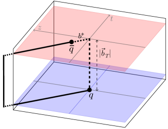
Figure 1: Graphs of the Wilson line structure of the $n$-collinear beam function $B_{q}$ (left) and the soft function $S^{q}$ (right), defined in eqs. (5) and (2.1). The Wilson lines (solid) extend to infinity in the directions indicated. Adapted from Ref. Li:2016axz .

At leading power (often referred to as twist-2), only three Dirac structures contribute to the TMDPDF:

$$\Gamma\in\{\,\not{{\bar{n}}}\,,\,\not{{\bar{n}}}\gamma_{5}\,,\,\mathrm{i}\sigma^{\alpha-}\gamma_{5}\,\}\,,$$ (8)

where $\sigma^{\mu\nu}=\frac{\mathrm{i}}{2}[\gamma^{\mu},\gamma^{\nu}]$. The resulting spin-dependent TMDs for a spin-$\frac{1}{2}$ hadron comprise eight independent Lorentz structures Ralston:1979ys ; Tangerman:1994eh ; Boer:1997nt ; Mulders:1995dh (see also Refs. Bacchetta:2004zf ; Goeke:2005hb ; Bacchetta:2006tn for a complete classification at higher orders in the power expansion, twist-3 and twist-4). Following the notation of Ref. Bacchetta:2006tn , the leading power decomposition in momentum space is

$$f_{q/h_{S}}^{[\not{{\bar{n}}}]}(x,\vec{q}_{T}) =f_{1}(x,q_{T})-\frac{\epsilon_{\rho\sigma}q_{\perp}^{\rho}S_{\perp}^{\sigma}}{M}f_{1T}^{\perp}(x,q_{T})\,,$$

$$f_{q/h_{S}}^{[\not{{\bar{n}}}\gamma_{5}]}(x,\vec{q}_{T}) =S_{L}\,g_{1L}(x,q_{T})-\frac{q_{\perp}\cdot S_{\perp}}{M}g_{1T}(x,q_{T})\,,$$

$$f_{q/h_{S}}^{[\mathrm{i}\sigma^{\alpha-}\gamma_{5}]}(x,\vec{q}_{T}) =S_{\perp}^{\alpha}h_{1}(x,q_{T})+\frac{S_{L}q_{\perp}^{\alpha}}{M}h_{1L}^{\perp}(x,q_{T})$$

$$\quad+\frac{q_{\perp}^{2}}{M^{2}}\biggl{(}\frac{1}{2}g_{\perp}^{\alpha\rho}-\frac{q_{\perp}^{\alpha}q_{\perp}^{\rho}}{q_{\perp}^{2}}\biggr{)}S_{\perp\,\rho}h_{1T}^{\perp}(x,q_{T})-\frac{\epsilon^{\alpha\rho}q_{\perp\rho}}{M}h_{1}^{\perp}(x,q_{T})\,.$$ (9)

Here, we drop the arguments $\mu$ and $\zeta$ for brevity. We also distinguish the position-space TMD $f_{q/h_{S}}^{[\Gamma]}(x,b_{T})$ and momentum-space TMD $f_{q/h_{S}}^{[\Gamma]}(x,\vec{q}_{T})$ only by their arguments. Note that all functions on the right-hand side of eq. (2.1) only depend on the magnitude $q_{T}=|\vec{q}_{T}|$ of the transverse momentum. In eq. (2.1), $M$ denotes the nucleon mass, $\alpha$ is a tranverse index, and the spin vector of the hadron $h$ is decomposed as

$$S^{\mu}=S_{L}\frac{P^{-}n^{\mu}-P^{+}{\bar{n}}^{\mu}}{2M}+S_{\perp}^{\mu}\,,$$ (10)

where $-S_{L}^{2}+S_{\perp}^{2}=-1$ such that $S^{2}=-1$. Eq. (2.1) contains eight distributions, which each correspond to a specific choice of polarizations for a quark and its parent hadron, as summarized in Table 1. Six of these distributions are time-reversal even (T-even); namely, the unpolarized ($f_{1})$, helicity ($g_{1L}$), transversity ($h_{1}$), pretzelosity ($h_{1T}^{\perp}$) and worm-gear ($g_{1T}$ and $h_{1L}^{\perp}$) distributions. The other two are T-odd; specifically, the Sivers ($f_{1T}^{\perp}$) Sivers:1989cc and Boer-Mulders ($h_{1}^{\perp}$) Boer:1997nt functions.

		Quark polarization
		U	L	T
Hadron polarization	U	$f_{1}$		$h_{1}^{\perp}$
		unpolarized		Boer-Mulders
	L		$g_{1L}$	$h_{1L}^{\perp}$
			helicity	worm-gear
	T	$f_{1T}^{\perp}$	$g_{1T}$	$h_{1}$, $h_{1T}^{\perp}$
		Sivers	worm-gear	transversity, pretzelosity

Table 1: Overview of the quark TMDs of a spin-$\frac{1}{2}$ hadron at leading power in eq. (2.1), organized by the polarization of the struck quark and the parent hadron. Here U, L, T stand for unpolarized, longitudinally polarized and transversely polarized, respectively. The Boer-Mulders and Sivers functions are time-reversal odd, while all other functions are time-reversal even.

One can obtain the position-space version of eq. (2.1) by a Fourier transform with respect to $\vec{q}_{T}$. As in Ref. Gutierrez-Reyes:2017glx , we normalize the position-space functions so that explicit factors of $M$ are absent. With this choice, we have

$$f_{q/h_{S}}^{[\not{{\bar{n}}}]}(x,\vec{b}_{T}) =f_{1}(x,b_{T})-\frac{\epsilon_{\rho\sigma}b_{\perp}^{\rho}S_{\perp}^{\rho}}{b_{T}}f_{1T}^{\perp}(x,b_{T})\,,$$

$$f_{q/h_{S}}^{[\not{{\bar{n}}}\gamma_{5}]}(x,\vec{b}_{T}) =S_{L}g_{1L}(x,b_{T})-\frac{b_{\perp}\cdot S_{\perp}}{b_{T}}g_{1T}(x,b_{T})\,,$$

$$f_{q/h_{S}}^{[\mathrm{i}{\bar{n}}_{\beta}\sigma^{\alpha\beta}\gamma_{5}]}(x,\vec{b}_{T}) =S_{\perp}^{\alpha}h_{1}(x,b_{T})+\frac{S_{L}b_{\perp}^{\alpha}}{b_{T}}h_{1L}^{\perp}(x,b_{T})$$

$$\quad+\biggl{(}\frac{1}{2}g_{\perp}^{\alpha\rho}-\frac{b_{\perp}^{\alpha}b_{\perp}^{\rho}}{b_{\perp}^{2}}\biggr{)}S_{\perp\,\rho}h_{1T}^{\perp}(x,b_{T})-\frac{\epsilon^{\alpha\rho}b_{\perp\rho}}{b_{T}}h_{1}^{\perp}(x,b_{T})\,,$$ (11)

where $b_{\perp}^{\mu}=(0,\vec{b}_{T},0)$ and $b_{T}=|\vec{b}_{T}|$. The explicit relations between position-space and momentum-space distributions are given by (see also Ref. Echevarria:2015uaa )

$$F(x,b_{T}) =2\pi\int_{0}^{\infty}\mathrm{d}k_{T}\,k_{T}J_{0}(b_{T}k_{T})F(x,k_{T})\,,\hskip 56.9055ptF\in\{f_{1},g_{1L},h_{1}\}$$

$$F(x,b_{T}) =2\pi\mathrm{i}\int_{0}^{\infty}\mathrm{d}k_{T}\,k_{T}\frac{k_{T}}{M}J_{1}(b_{T}k_{T})F(x,k_{T})\,,\hskip 38.69576ptF\in\{f_{1T}^{\perp},g_{1T},h_{1L}^{\perp},h_{1}^{\perp}\}$$

$$h_{1T}^{\perp}(x,b_{T}) =-2\pi\int_{0}^{\infty}\mathrm{d}k_{T}\,k_{T}\frac{k_{T}^{2}}{M^{2}}J_{2}(b_{T}k_{T})h_{1T}^{\perp}(x,k_{T})\,,$$ (12)

where $J_{n}(x)$ is a Bessel function of the first kind. Note that only $f_{1}$, $g_{1L}$ and $h_{1}$ are directly related by a Fourier transform to their momentum-space counterparts. The remaining functions require higher-order Bessel transforms reweighted with an appropriate factor of $(k_{T}/M)$ or $(k_{T}/M)^{2}$, due to the normalization conventions in eq. (2.1).

2.2 Definition of spin-dependent quasi-TMDPDFs

Within the framework of LaMET Ji:2013dva ; Ji:2014gla , quasi-TMDPDFs are defined as equal-time analogs of TMDPDFs, and are thus amenable to lattice calculations. To define the spin-dependent quasi-TMDPDFs, we extend the setup in  Ref. Ebert:2019okf :

$$\tilde{f}_{q/h_{S}}^{[\tilde{\Gamma}]}(x,\vec{b}_{T},\mu,P^{z})=\int\frac{\mathrm{d}b^{z}}{2\pi}\,e^{\mathrm{i}b^{z}(xP^{z})}\, \tilde{Z}^{\prime}_{q}(b^{z},\mu,\tilde{\mu})\tilde{Z}_{\rm uv}^{q}(b^{z},\tilde{\mu},a)$$

$$\times\tilde{B}_{q/h_{S}}^{[\tilde{\Gamma}]}(b^{z},\vec{b}_{T},a,L,P^{z})\tilde{\Delta}_{S}^{q}(b_{T},a,L)\,.$$ (13)

Here, $h_{S}$ denotes a hadron with spin $S$ and momentum $P$, $q$ is the flavor of the struck quark, $x$ is the fraction of the $z$-momentum carried by this quark, and $\vec{b}_{T}$ is Fourier-conjugate to the quark’s transverse momentum. The scale $\mu$ is the ${\overline{\mathrm{MS}}}$-renormalization scale, and the $P^{z}$ dependence here plays the role of the Collins-Soper scale $\zeta$. Moreover, $\tilde{B}_{q/h_{S}}^{[\tilde{\Gamma}]}$ and $\tilde{\Delta}_{S}^{q}$ denote the quasi beam function and quasi soft factor.

For the purposes of this paper, we need not go into details about the precise definition of $\tilde{\Delta}_{S}^{q}$; while we must include it in the quasi beam function to cancel $L/b_{T}$ divergences, it cancels out when taking the ratio of two quasi-TMDPDFs. In eq. (2.2) the letter $a$ denotes the UV regulator, resembling the notation for the lattice spacing that acts as a UV regulator in practical calculations. Here the rapidity regulator is replaced by the dependence on the length $L$ of the staple-shaped Wilson lines defined below Ji:2018hvs ; Ebert:2019okf . In contrast to eq. (2.1), we formulate the UV renormalization in eq. (2.2) in $b^{z}$ space, where the lattice renormalization factor $\tilde{Z}_{\rm uv}^{q}$ absorbs Wilson-line self energies proportional to $b^{z}$, with $\tilde{\mu}$ being the corresponding renormalization scale. Finally, $\tilde{Z}_{q}^{\prime}$ converts this lattice-renormalization scheme into the ${\overline{\mathrm{MS}}}$ scheme. For more details, we refer to Refs. Ebert:2019okf ; Ebert:2019tvc .

We define the quasi beam function in position space as

$$\tilde{B}_{q/h_{S}}^{[\tilde{\Gamma}]}(b^{z},\vec{b}_{T},a,L,P^{z}) =N_{\tilde{\Gamma}}\,\Bigl{<}h_{S}(P)\Big{|}\bar{q}(b^{\mu})\widetilde{W}_{\sqsubset}(b^{\mu},0;L)\frac{\tilde{\Gamma}}{2}q(0)\Big{|}h_{S}(P)\Bigr{>}\,,$$ (14)

where $h_{S}(P)$ denotes a hadron $h$ with polarization vector $S$ and momentum $P$, and $b^{\mu}=(0,\vec{b}_{T},b^{z})$. Here we follow Ref. Ebert:2019okf . $\widetilde{W}_{\sqsubset}(b^{\mu},0;L)$ is a staple-shaped Wilson line path of length $L$ connecting the quark fields, as illustrated in the left panel of Fig. 2; it is given by

$$\widetilde{W}_{\sqsubset}(b^{\mu},0;L) =W_{\hat{z}}(b^{\mu};L-b^{z})W_{T}(L\hat{z};\vec{b}_{T},\vec{0}_{T})W^{\dagger}_{\hat{z}}(0;L)\,,$$ (15)

where $W_{T}$ is given in eq. (2.1) and $W_{\hat{z}}$ denotes a Wilson line oriented along the $z$-direction,

$$W_{\hat{z}}(x^{\mu};L) =P\exp\left[\mathrm{i}g\int_{L}^{0}\mathrm{d}s\,\mathcal{A}^{z}(x^{\mu}+s\hat{z})\right]\,.$$ (16)

The Dirac structures $\tilde{\Gamma}$ come from the set

$$\tilde{\Gamma}\in\{\,\gamma^{\lambda}\,,\,\gamma^{\lambda}\gamma_{5}\,,\,\mathrm{i}\sigma^{\alpha\lambda}\gamma_{5}\,\}\,,\qquad\lambda=0,3\,,$$ (17)

because they can be boosted to the three corresponding Dirac structures in eq. (8). The normalization factor $N_{\tilde{\Gamma}}$ in eq. (14) is defined as

$$N_{\gamma^{3}}=N_{\gamma^{0}\gamma_{5}}=N_{i\sigma^{i3}\gamma_{5}}=1\,,\qquad N_{\gamma^{0}}=N_{\gamma^{3}\gamma_{5}}=N_{i\sigma^{i0}\gamma_{5}}=\frac{P^{z}}{P^{0}}\,.$$ (18)

While the choices $\lambda=0$ and $\lambda=3$ are formally equivalent in a continuum analysis, they induce different operator mixings on a discretized lattice with broken chiral symmetry Constantinou:2019vyb ; Shanahan:2019zcq ; Green:2020xco . Hence, we consider both options.

Since all choices in eq. (17) boost onto the corresponding Dirac structures in eq. (8), we can decompose the quasi-TMDs in the same fashion as the TMDs, up to power corrections suppressed by large $P^{z}$. Using the conventions of eq. (2.1), at leading power we find

$$\tilde{f}_{q/h_{S}}^{[\gamma^{\lambda}]}(x,\vec{b}_{T}) =\tilde{f}_{1}^{\lambda}(x,b_{T})-\frac{\epsilon_{\rho\sigma}b_{\perp}^{\rho}S_{\perp}^{\sigma}}{b_{T}}\tilde{f}_{1T}^{\lambda\perp}(x,b_{T})\,,$$

$$\tilde{f}_{q/h_{S}}^{[\gamma^{\lambda}\gamma_{5}]}(x,\vec{b}_{T}) =S_{L}\tilde{g}_{1L}^{\lambda}(x,b_{T})-\frac{b_{\perp}\cdot S_{\perp}}{b_{T}}\tilde{g}_{1T}^{\lambda}(x,b_{T})\,,$$

$$\tilde{f}_{q/h_{S}}^{[\mathrm{i}\sigma^{\alpha\lambda}\gamma_{5}]}(x,\vec{b}_{T}) =S_{\perp}^{\alpha}\tilde{h}_{1}^{\lambda}(x,b_{T})+\frac{S_{L}b_{\perp}^{\alpha}}{b_{T}}\tilde{h}_{1L}^{\lambda\perp}(x,b_{T})$$

$$\quad+\biggl{(}\frac{1}{2}g_{\perp}^{\alpha\rho}-\frac{b_{\perp}^{\alpha}b_{\perp}^{\rho}}{b_{\perp}^{2}}\biggr{)}S_{\perp\,\rho}\tilde{h}_{1T}^{\lambda\perp}(x,b_{T})-\frac{\epsilon^{\alpha\rho}b_{\perp\rho}}{b_{T}}\tilde{h}_{1}^{\lambda\perp}(x,b_{T})\,.$$ (19)

By choosing the appropriate projector $\tilde{\Gamma}$ and hadron polarization $S$, it is straightforward to obtain all individual distributions.

Each Wilson line segment gives rise to a power-law divergence proportional to its length due to self-energy contributions Dotsenko:1979wb ; Craigie:1980qs ; Dorn:1986dt . As argued in Ref. Ebert:2019tvc ; Green:2020xco , the nonlocal Wilson line operator that defines the quasi beam function can be multiplicatively renormalized by the factor

$$Z(b^{z},\tilde{\mu},a,b_{T},L)=Z_{q,\rm wf}(\tilde{\mu},a)\,e^{\delta m(2L-b^{z}+b_{T})}\,,$$ (20)

where $\delta m=\delta m(a)\sim 1/a$ absorbs the power-law dviergence originating from each Wilson line segment, and $Z_{q,\rm wf}(\tilde{\mu},a)$ renormalizes all logarithmic UV divergences from the wave functions and quark-Wilson-line vertices. Thus the $Z$ factor is independent of $\tilde{\Gamma}$. The $b^{z}$ dependence in eq. (20) induces the presence of $b^{z}$ in $\tilde{Z}_{\rm uv}^{q}(b^{z},\tilde{\mu},a)$ in eq. (2.2), since subtracting the self energies on the lattice necessitates the use of a $b^{z}$-dependent counterterm. This also leads to a $b^{z}$-dependent factor $\tilde{Z}_{q}^{\prime}(b^{z},\mu,\tilde{\mu})$ to convert to the ${\overline{\mathrm{MS}}}$ scheme.

To avoid this complication, we can slightly modify the definition in eq. (15) so that the length of the Wilson line path is independent of $b^{z}$. We can achieve this either by shifting $L\to L+b^{z}/2$ in eq. (15), or equivalently by using the definition of Refs. Ji:2019ewn ; Ji:2020ect ,

$$\tilde{B}_{q}^{[\tilde{\Gamma}]}(b^{z},\vec{b}_{T},a,L,P^{z}) =N_{\tilde{\Gamma}}\,\Bigl{<}h_{S}(P)\Big{|}\bar{q}\Bigl{(}b_{\perp}+\frac{b^{z}}{2}\hat{z}\Bigr{)}\widetilde{W}_{\sqsubset}\Bigl{(}b_{\perp}+\frac{b^{z}}{2}\hat{z},-\frac{b^{z}}{2}\hat{z};L+\frac{b^{z}}{2}\Bigr{)}\,,$$

$$\qquad\qquad\qquad\ \times\frac{\tilde{\Gamma}}{2}q\Bigl{(}-\frac{b^{z}}{2}\hat{z}\Bigr{)}\Big{|}h_{S}(P)\Bigr{>}\,.$$ (21)

We illustrate this modified path in the right panel of Fig. 2. The operator in eq. (14) keeps the position of one quark field fixed so that only one Wilson line is varied for each choice of $b^{z}$ on the lattice, whereas all three of the Wilson lines are varied for the operator in eq. (2.2).

Importantly, eqs. (15) and (2.2) are equivalent in the limit $L\gg b^{z}$; thus, all results expanded in this limit apply to both definitions. The RI/MOM^′ renormalization factor calculated at one loop in Ref. Ebert:2019tvc applies directly to eq. (15), and can be applied to eq. (2.2) after a shift $L\to L+b^{z}/2$.

A key benefit of using the definition in eq. (2.2) is that the renormalization factors in eq. (2.2) become independent of $b^{z}$ and can be extracted from the Fourier transform, giving us

$$\tilde{f}_{q/h_{S}}^{[\tilde{\Gamma}]}(x,\vec{b}_{T},\mu,P^{z}) =\lim_{\begin{subarray}{c}a\to 0\\ L\to\infty\end{subarray}}\tilde{Z}_{q}(\mu,a)\tilde{B}_{q/h_{S}}^{[\tilde{\Gamma}]}(x,\vec{b}_{T},a,L,P^{z})\tilde{\Delta}_{S}^{q}(b_{T},a,L)\,,$$

$$\tilde{B}_{q/h_{S}}^{[\tilde{\Gamma}]}(x,\vec{b}_{T},a,L,P^{z}) =\int\frac{\mathrm{d}b^{z}}{2\pi}e^{\mathrm{i}b^{z}(xP^{z})}\tilde{B}_{q/h_{S}}^{[\tilde{\Gamma}]}(b^{z},\vec{b}_{T},a,L,P^{z})\,.$$ (22)

Here $\tilde{Z}_{q}(\mu,a)=\tilde{Z}^{\prime}_{q}(\mu,\tilde{\mu})\tilde{Z}_{\rm uv}^{q}(\tilde{\mu},a)$ is the $b^{z}$-independent combination of lattice renormalization and ${\overline{\mathrm{MS}}}$ conversion factors. Alternatively, one could of course also apply the renormalization and soft subtraction prior to the Fourier transform. Moreover, $\tilde{Z}_{q}(\mu,a)$ will drop out in the ratios of quasi-TMDPDFs, further simplifying the calculation. Appendix A discusses using eq. (2.2) for calculating the Collins-Soper kernel.

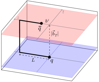
Figure 2: Illustration of the Wilson line structure of the quasi beam function $\tilde{B}_{q}$ as defined in eq. (15) (left) and eq. (2.2) (right).

2.3 Relating quasi-TMDPDFs and TMDPDFs

Following the notation of Ref. Ebert:2019okf , we write the relation between TMDs and quasi-TMDs as

$$\tilde{F}_{{\rm ns}/h_{S}}(x,b_{T},\mu,P^{z}) =C^{\tilde{F}}_{{\rm ns}}\bigl{(}\mu,xP^{z}\bigr{)}g^{S}_{q}(b_{T},\mu)\exp\biggl{[}\frac{1}{2}\gamma_{\zeta}^{q}(\mu,b_{T})\ln\frac{(2xP^{z})^{2}}{\zeta}\biggr{]}F_{{\rm ns}/h_{S}}(x,b_{T},\mu,\zeta)$$

$$\quad+\mathcal{O}\biggl{(}\frac{b_{T}}{L},\frac{1}{b_{T}P^{z}},\frac{1}{P^{z}L}\biggr{)}\,.$$ (23)

Here, $F$ can be any of the spin-dependent TMDs in eq. (2.1), $\tilde{F}$ is the corresponding quasi-TMD, and the nonsinglet combination $ns=u{-}d$ is chosen to avoid mixing with gluons. Notably, the relation between TMDs and quasi-TMDs is multiplicative in $x$ space, with $C_{{\rm ns}}^{\tilde{F}}$ being a perturbative kernel. It also involves the nonperturbative Collins-Soper evolution to render the right-hand side independent of $\zeta$ for situations where $\zeta\neq(2xP^{z})^{2}$, such as when the quasi-TMD and TMD have different values for $P^{z}$. In addition, following Ref. Ebert:2019okf we have included in eq. (2.3) a nonperturbative factor $g_{q}^{S}(b_{T},\mu)$ which ensures that this relation is independent of the precise choice for the quasi soft function $\tilde{\Delta}_{S}^{q}(b_{T},a,L)$ in eq. (2.2). (See Refs. Ji:2019ewn ; Ji:2020ect ; Vladimirov:2020ofp for discussions of this structure.) The precise choice for $\tilde{\Delta}_{S}^{q}$, and thus $g_{q}^{S}$, is irrelevant for ratios of TMDs and quasi-TMDs, and thus does not impact our results. Eq. (2.3) is correct up to corrections suppressed by large momenta $P^{z}$ and staple lengths $L$, as indicated.

We consider ratios of eq. (2.3) with different TMDs, such that the spin-independent Collins-Soper evolution and $g_{q}^{S}$ cancel. For example, division by the unpolarized TMD gives

$$\frac{\tilde{F}_{{\rm ns}/h_{S}}(x,b_{T},\mu,P^{z})}{\tilde{f}_{{\rm ns}}(x,b_{T},\mu,P^{z})} =\frac{C^{\tilde{F}}_{{\rm ns}}\bigl{(}\mu,xP^{z}\bigr{)}}{C_{{\rm ns}}\bigl{(}\mu,xP^{z}\bigr{)}}\frac{F_{{\rm ns}/h_{S}}(x,b_{T},\mu,\zeta)}{f(x,b_{T},\mu,\zeta)}\,,$$ (24)

up to power-suppressed terms. Ref. Ebert:2019okf gives the kernel appearing in the denominator:

$$C_{{\rm ns}}\bigl{(}\mu,xP^{z}\bigr{)} =1+\frac{\alpha_{s}C_{F}}{4\pi}\biggl{[}-\ln^{2}\frac{(2xP^{z})^{2}}{\mu^{2}}+2\ln\frac{(2xP^{z})^{2}}{\mu^{2}}-4+\frac{\pi^{2}}{6}\biggr{]}+\mathcal{O}(\alpha_{s}^{2})\,.$$ (25)

A main goal of our work here will be to determine results for the kernels $C^{\tilde{F}}_{{\rm ns}}\bigl{(}\mu,xP^{z}\bigr{)}$ appearing in the numerator.

Another advantage of eq. (24) is that the soft factor $\tilde{\Delta}_{S}^{q}$ contained in the quasi-TMDs, see eq. (2.2), also cancels in the ratio. We may thus equally well write

$$\frac{\tilde{B}_{{\rm ns}/h_{S}}(x,b_{T},\mu,P^{z})}{\tilde{B}_{{\rm ns}}(x,b_{T},\mu,P^{z})} =\frac{C^{\tilde{F}}_{{\rm ns}}\bigl{(}\mu,xP^{z}\bigr{)}}{C_{{\rm ns}}\bigl{(}\mu,xP^{z}\bigr{)}}\frac{F_{{\rm ns}/h_{S}}(x,b_{T},\mu,\zeta)}{f(x,b_{T},\mu,\zeta)}\,,$$ (26)

where $\tilde{B}_{{\rm ns}/h_{S}}$ and $\tilde{B}_{\rm ns}$ are the beam functions that give rise to the spin-dependent and unpolarized quasi-TMDs $\tilde{F}_{\rm ns}$ and $\tilde{f}_{\rm ns}$, respectively.

3 One-loop calculation

With the required formalism in place, we now turn to the calculation of the matching kernel $C_{\rm ns}^{\tilde{F}}$ appearing in eq. (2.3). Since the matching results are independent of the precise choice of states, as long as they have overlap with the operators, we can carry out the calculation of the matrix elements in eqs. (5) and (14) using an on-shell quark state $u_{s}(p)$ with spin vector $s$ and momentum $p^{\mu}=p^{-}n^{\mu}/2$, where $p^{-}=2p^{0}=2p^{z}$. The following on-shell relations greatly simplify the calculation:

$$\not{p}\,u_{s}(p)=\bar{u}_{s}(p)\,\not{p}=0\,,\qquad P_{n}u_{s}(p)=u_{s}(p)\,,\qquad\bar{u}_{s}(p)P_{\bar{n}}=\bar{u}_{s}(p)\,,$$ (27)

where $P_{n}=\not{n}\not{{\bar{n}}}/4$ and $P_{\bar{n}}=\not{{\bar{n}}}\not{n}/4$ are projectors. We employ Feynman gauge and regulate both infrared (IR) and UV divergences by working in $d=4-2\epsilon$ dimensions. We note that in this setup, both the unpolarized TMDPDF and unpolarized quasi-TMDPDF already exist in the literature, which provides a useful reference for our analysis.

Notation.

We work exclusively in Fourier space, with $b_{\perp}^{\mu}=(0,\vec{b}_{T},0)$ Fourier conjugate to $q_{T}^{\mu}=(0,\vec{q}_{T},0)$, and $b_{\perp}^{2}=-\vec{b}_{T}^{2}$. We define a shorthand for the canonical logarithm that appears as

$$L_{b}=\ln\frac{\vec{b}_{T}^{2}\mu^{2}}{b_{0}^{2}}\,,\qquad b_{0}=2e^{-\gamma_{E}}\,,$$ (28)

where $\gamma_{E}$ is the Euler-Mascheroni constant. We express all our results in the ${\overline{\mathrm{MS}}}$ scheme. The associated renormalization scale $\mu$ is related to the MS scale $\mu_{0}$ by $\mu^{2}=4\pi e^{-\gamma_{E}}\mu_{0}^{2}$.

3.1 Tree-level results

The tree-level results for the TMDPDF and quasi-TMDPDF are

$$f_{q/h_{S}}^{[\Gamma]\,(0)}(x,\vec{b}_{T},\mu,\zeta) =\frac{1}{p^{-}}\mathrm{Tr}\biggl{[}u_{s}(p)\bar{u}_{s}(p)\frac{\Gamma}{2}\biggr{]}\delta(1-x)\,,$$

$$\tilde{f}_{q/h_{S}}^{[\tilde{\Gamma}]\,(0)}(x,\vec{b}_{T},\mu,p^{z}) =\frac{N_{\Gamma}}{p^{z}}\mathrm{Tr}\biggl{[}u_{s}(p)\bar{u}_{s}(p)\frac{\tilde{\Gamma}}{2}\biggr{]}\delta(1-x)\,.$$ (29)

For the case of a massless spinor $N_{\tilde{\Gamma}}=1$ (i.e. independent of $\tilde{\Gamma}$), the completeness relation reads:

$$u_{s}(p)\bar{u}_{s}(p)=\frac{1}{2}\,\not{p}\,(1-\Lambda\gamma_{5}+\gamma_{5}\not{s}_{\perp})\,,$$ (30)

where $\Lambda$ is the helicity and $s_{\perp}$ is the transverse polarization vector. (See Ref. Barone:2001sp for a review of polarization with spinors.) Thus, the traces in eq. (3.1) give

$$\Gamma=\gamma^{\lambda}:\qquad \mathrm{Tr}\Bigl{[}u_{s}(p)\bar{u}_{s}(p)\frac{\gamma^{\lambda}}{2}\Bigr{]} =p^{\lambda}\,,$$

$$\Gamma=\gamma^{\lambda}\gamma_{5}:\qquad \mathrm{Tr}\Bigl{[}u_{s}(p)\bar{u}_{s}(p)\frac{\gamma^{\lambda}\gamma_{5}}{2}\Bigr{]} =\Lambda p^{\lambda}\,,$$

$$\Gamma=\mathrm{i}\sigma^{\alpha\lambda}\gamma_{5}:\qquad \mathrm{Tr}\Bigl{[}u_{s}(p)\bar{u}_{s}(p)\frac{\mathrm{i}\sigma^{\alpha\lambda}\gamma_{5}}{2}\Bigr{]} =p^{\lambda}s_{\perp}^{\alpha}\,.$$ (31)

Comparing to the decompositions in eqs. (2.1) and (2.2), we see that only the unpolarized ($f_{1}$ and $\tilde{f}_{1}$), helicity ($g_{1L}$ and $\tilde{g}_{1L}$) and transversity ($h_{1}$ and $\tilde{h}_{1}$) TMD and quasi-TMDs are nonzero at tree level. Moreover, by definition these functions are normalized to $\delta(1-x)$ at tree level. This implies that

$$C_{\rm ns}^{\tilde{f}_{1}}=C_{\rm ns}^{\tilde{g}_{1L}}=C_{\rm ns}^{\tilde{h}_{1}}=1+{\cal O}(\alpha_{s})\,.$$ (32)

It is instructive to carry out the same analysis using massive quarks. In this case, the completeness relation is

$$u_{s}(p)\bar{u}_{s}(p)=(\not{p}+m)\frac{1}{2}(1+\gamma_{5}\not{s})\,,$$ (33)

and the Dirac traces in eq. (3.1) evaluate to (in $d=4$ dimensions)

$$\Gamma=\gamma^{\lambda}:\qquad \mathrm{Tr}\Bigl{[}u_{s}(p)\bar{u}_{s}(p)\frac{\gamma^{\lambda}}{2}\Bigr{]} =p^{\lambda}\,,$$

$$\Gamma=\gamma^{\lambda}\gamma_{5}:\qquad \mathrm{Tr}\Bigl{[}u_{s}(p)\bar{u}_{s}(p)\frac{\gamma^{\lambda}\gamma_{5}}{2}\Bigr{]} =ms^{\lambda}\,,$$

$$\Gamma=\mathrm{i}\sigma^{\alpha\lambda}\gamma_{5}:\qquad \mathrm{Tr}\Bigl{[}u_{s}(p)\bar{u}_{s}(p)\frac{\mathrm{i}\sigma^{\alpha\lambda}\gamma_{5}}{2}\Bigr{]} =p^{\lambda}s^{\alpha}-p^{\alpha}s^{\lambda}=p^{\lambda}s_{\perp}^{\alpha}\,.$$ (34)

In the last equation, we used that $p^{\alpha}=0$ since $\alpha$ is a transverse index. From eq. (10) $ms^{0}=p^{z}$ and $ms^{3}=p^{0}$, and using our definition of $N_{\tilde{\Gamma}}$ in eq. (18), we find that both the TMD and the quasi-TMD are again normalized to $\delta(1-x)$ at tree level. This result confirms the choices made in eq. (18).

3.2 TMDPDFs

To carry out the matching calculation to ${\cal O}(\alpha_{s})$ requires comparing one-loop results for the spin-dependent TMDPDF and quasi-TMDPDF. Here we present the one-loop results for the spin-dependent TMDPDF, which requires us to combine the spin-dependent beam function at one-loop with the standard TMD soft function at the same order. Both the beam and the soft function are individually rapidity divergent, and we choose to employ the $\eta$ regulator of Refs. Chiu:2011qc ; Chiu:2012ir to regulate these divergences.

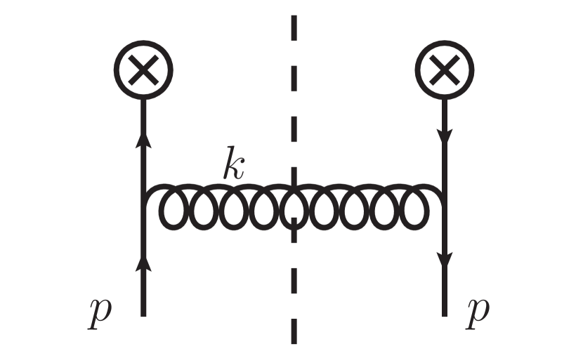
(a)

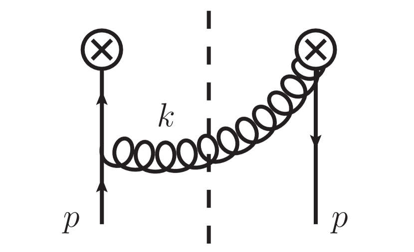
(b)

Figure 3: One-loop diagrams contributing to the spin-dependent beam function in eq. (5). Mirror diagrams and the scaleless wave function and tadpole diagrams are not shown. The dashed line indicates the on-shell constraint on the emitted gluon. The $\otimes$ denotes the two Wilson line operators.

Spin-dependent beam function.

There are only two diagrams that do not vanish in dimensional regularization, as shown in Fig. 3. Note that in the lightlike case, the transverse Wilson line does not contribute in nonsingular gauges, such as the Feynman gauge we employ here. Rapidity divergences for the phase space integral over $k$ are regulated by the factors of $|k^{-}/\nu|^{-\eta}$ appearing from the regulated Wilson lines, after which the calculation is straightforward. We obtain

$$q_{A}^{\Gamma\,(1)}(x,\vec{b}_{T}) =\frac{1}{p^{-}}\bigl{[}\bar{u}_{s}^{a}(p)u_{s}^{b}(p)\bigr{]}\,\frac{\alpha_{s}C_{F}}{4\pi}\frac{\Gamma(-\epsilon)}{e^{\epsilon\gamma_{E}}}e^{\epsilon L_{b}}\Bigl{(}\gamma^{\mu}\gamma_{\alpha}\frac{\Gamma}{2}\gamma_{\beta}\gamma_{\mu}\Bigr{)}^{ab}$$

$$~{}\quad\times\left[-\mathrm{i}\epsilon\frac{{\bar{n}}^{\alpha}b_{\perp}^{\beta}+{\bar{n}}^{\beta}b_{\perp}^{\alpha}}{p^{-}b_{\perp}^{2}}+(1-x)\left(\frac{g_{\perp}^{\alpha\beta}}{2}+\epsilon\frac{b_{\perp}^{\alpha}b_{\perp}^{\beta}}{b_{\perp}^{2}}\right)\right]\,,$$ (35)

$$q_{B}^{\Gamma\,(1)}(x,\vec{b}_{T}) =\frac{1}{p^{-}}\bigl{[}\bar{u}_{s}^{a}(p)u_{s}^{b}(p)\bigr{]}\frac{\alpha_{s}C_{F}}{4\pi}\frac{\Gamma(-\epsilon)}{e^{\epsilon\gamma_{E}}}e^{\epsilon L_{b}}\biggl{\{}-\bigl{(}P_{\bar{n}}\Gamma+\Gamma P_{n}\bigr{)}^{ab}+\Bigl{[}\mathcal{L}_{0}(1-x)$$

$$~{}\quad+\delta(1-x)\Bigl{(}-\frac{1}{\eta}+\ln\frac{p^{-}}{\nu}\Bigr{)}\Bigr{]}\biggl{[}\bigl{(}P_{\bar{n}}\Gamma+\Gamma P_{n}\bigr{)}-\mathrm{i}\epsilon\frac{\not{{\bar{n}}}\not{b}_{\perp}\Gamma}{p^{-}b_{\perp}^{2}}-\mathrm{i}\epsilon\frac{\Gamma\not{b}_{\perp}\not{{\bar{n}}}}{p^{-}b_{\perp}^{2}}\biggr{]}^{ab}\biggr{\}}\,,$$ (36)

where $\mathcal{L}_{0}(1-x)=[1/(1-x)]_{+}$ is the standard plus distribution. Since the graph leading to eq. (3.2) is rapidity finite it does not depend on the rapidity regulator. In eq. (3.2) the rapidity divergence is explicit through the $1/\eta$ pole in the rapidity regulator $\eta$, with $\ln(p^{-}/\nu)$ the associated rapidity logarithm. Here, we have already expanded in $\eta\to 0$, while keeping the exact $\epsilon$ dependence.

Both eqs. (3.2) and (3.2) contain Dirac structures that scale as $1/(p^{-}b_{\perp}^{2})$. We can neglect these terms in the limit of large $p^{-}\to\infty$, which is also why they do not appear in the decomposition in eq. (2.1). Using eq. (27), we obtain

$$B_{q/h_{S}}^{[\Gamma]}(x,\vec{b}_{T},\epsilon,p^{-}/\nu) =\frac{1}{p^{-}}\bigl{[}\bar{u}_{s}^{a}(p)u_{s}^{b}(p)\bigr{]}\frac{\Gamma^{ab}}{2}\delta(1-x)+\frac{1}{p^{-}}\bigl{[}\bar{u}_{s}^{a}(p)u_{s}^{b}(p)\bigr{]}\,\frac{\alpha_{s}C_{F}}{4\pi}\frac{\Gamma(-\epsilon)}{e^{\epsilon\gamma_{E}}}e^{\epsilon L_{b}}$$

$$\quad\times\biggl{\{}\frac{\Gamma^{ab}}{2}\Bigl{[}4\mathcal{L}_{0}(1-x)+4\delta(1-x)\Bigl{(}-\frac{1}{\eta}+\ln\frac{p^{-}}{\nu}\Bigr{)}-4\Bigr{]}$$

$$\qquad+\Bigl{(}\gamma^{\mu}\gamma_{\alpha}\frac{\Gamma}{2}\gamma_{\beta}\gamma_{\mu}\Bigr{)}^{ab}(1-x)\biggl{(}\frac{g_{\perp}^{\alpha\beta}}{2}+\epsilon\frac{b_{\perp}^{\alpha}b_{\perp}^{\beta}}{b_{\perp}^{2}}\biggr{)}\biggr{\}}+\mathcal{O}(\alpha_{s}^{2})\,.$$ (37)

Soft function.

From Refs. Chiu:2012ir ; Luebbert:2016itl the bare soft function with the $\eta$ regulator is

$$S_{q}(b_{T},\epsilon,\nu)=1+\frac{\alpha_{s}C_{F}}{4\pi}\frac{\Gamma(-\epsilon)}{e^{\epsilon\gamma_{E}}}e^{\epsilon L_{b}}\biggl{[}\frac{8}{\eta}+4L_{b}+8\ln\frac{\nu}{\mu}-4\gamma_{E}-4\psi(-\epsilon)\biggr{]}+\mathcal{O}(\alpha_{s}^{2})\,,$$ (38)

where $\psi(x)=\Gamma^{\prime}(x)/\Gamma(x)$ is the digamma function.

Spin-dependent TMDPDF.

When using the $\eta$ regulator, the zero bin is scaleless and vanishes. Thus, the bare spin-dependent TMDPDF is

$$f_{q/h_{S}}^{[\Gamma]}(x,\vec{b}_{T},\epsilon,\zeta) =B_{q/h_{S}}^{[\Gamma]}\bigl{(}x,\vec{b}_{T},\epsilon,\sqrt{\zeta}/\nu\bigr{)}\sqrt{S_{q}(b_{T},\epsilon,\nu)}$$

$$=\frac{1}{p^{-}}\bigl{[}\bar{u}^{a}_{s}(p)u_{s}^{b}(p)\bigr{]}\frac{\Gamma^{ab}}{2}\delta(1-x)+\frac{1}{p^{-}}\bigl{[}\bar{u}_{s}^{a}(p)u_{s}^{b}(p)\bigr{]}\,\frac{\alpha_{s}C_{F}}{4\pi}\frac{\Gamma(-\epsilon)}{e^{\epsilon\gamma_{E}}}e^{\epsilon L_{b}}$$

$$\quad\times\biggl{\{}\frac{\Gamma^{ab}}{2}\Bigl{[}4\mathcal{L}_{0}(1-x)+2\delta(1-x)\Bigl{(}L_{b}+\ln\frac{\zeta}{\mu^{2}}-\gamma_{E}-\psi_{-\epsilon}\Bigr{)}-4\Bigr{]}$$

$$\qquad+\Bigl{(}\gamma^{\mu}\gamma_{\alpha}\frac{\Gamma}{2}\gamma_{\beta}\gamma_{\mu}\Bigr{)}^{ab}(1-x)\biggl{(}\frac{g_{\perp}^{\alpha\beta}}{2}+\epsilon\frac{b_{\perp}^{\alpha}b_{\perp}^{\beta}}{b_{\perp}^{2}}\biggr{)}\biggr{\}}+\mathcal{O}(\alpha_{s}^{2})\,.$$ (39)

This result agrees with Ref. Gutierrez-Reyes:2017glx after accounting for different conventions.

It is convenient to note that eq. (3.2) has a universal structure because large parts of the NLO correction have the same Dirac structure as the tree level result. To make this explicit, we write eq. (3.2) as

$$f_{q/h_{S}}^{[\Gamma]}(x,\vec{b}_{T},\epsilon,\zeta) =\frac{1}{p^{-}}\Bigl{[}\bar{u}_{s}(p)\frac{\Gamma}{2}u_{s}(p)\Bigr{]}\Bigl{[}\delta(1-x)+\frac{\alpha_{s}C_{F}}{4\pi}f_{b}^{(1)}\Bigr{]}$$

$$\quad+\frac{\alpha_{s}C_{F}}{4\pi}\frac{1}{p^{-}}\Bigl{[}\bar{u}_{s}(p)\gamma^{\mu}\gamma_{\alpha}\frac{\Gamma}{2}\gamma_{\beta}\gamma_{\mu}u_{s}(p)\Bigr{]}\biggl{[}f^{(1)}_{a1}\frac{g_{\perp}^{\alpha\beta}}{2}+f^{(1)}_{a2}\Bigl{(}\frac{g_{\perp}^{\alpha\beta}}{2}-\frac{b_{\perp}^{\alpha}b_{\perp}^{\beta}}{b_{\perp}^{2}}\Bigr{)}\biggr{]}$$

$$\quad+\mathcal{O}(\alpha_{s}^{2})\,,$$ (40)

where the coefficient functions $f_{i}^{(1)}$, whose arguments we keep implicit, are given by

$$f^{(1)}_{b} =\Bigl{(}\frac{1}{\epsilon_{\rm IR}}+L_{b}\Bigr{)}\bigl{[}-2P_{qq}(x)+2(1-x)\bigr{]}$$

$$\quad+\delta(1-x)\biggl{[}\frac{2}{\epsilon^{2}}+\Bigl{(}\frac{1}{\epsilon}+L_{b}\Bigr{)}\Bigl{(}-2\ln\frac{\zeta}{\mu^{2}}+3\Bigr{)}-L_{b}^{2}-\frac{\pi^{2}}{6}\biggr{]}+\mathcal{O}(\epsilon)\,,$$

$$f^{(1)}_{a1} =-(1-x)\Bigl{[}\frac{1}{\epsilon_{\rm IR}}+L_{b}+1+\mathcal{O}(\epsilon)\Bigr{]}\,,$$

$$f^{(1)}_{a2} =(1-x)+\mathcal{O}(\epsilon)\,.$$ (41)

Here, $\epsilon_{\rm IR}$ denotes poles of IR origin, while $\epsilon$ denotes poles of UV origin. The unpolarized splitting function is given by

$$P_{qq}(x)=\biggl{(}\frac{1+x^{2}}{1-x}\biggr{)}_{+}=2\mathcal{L}_{0}(1-x)+\frac{3}{2}\delta(1-x)-(1+x)\,.$$ (42)

In eq. (3.2), $f_{b}^{(1)}$ arises entirely from diagram (b) and the soft subtraction, whereas the two distinct Lorentz structures of $f_{a1}^{(1)}$ and $f_{a2}^{(1)}$ result from diagram (a). Eqs. (3.2) and (3.2) reveal that at NLO, the full distributional structure in $x$ of the spin-dependent TMDPDF is proportional to the tree-level normalization and is thus universal. The true dependence on $\Gamma$ is always proportional to $(1-x)$. This also explains the similar kernels that appear when perturbatively matching the spin-dependent TMD onto spin-dependent PDFs, see Refs. Bacchetta:2013pqa ; Echevarria:2015uaa ; Gutierrez-Reyes:2017glx .

For any desired Dirac structure $\Gamma$, it is straightforward to insert this $\Gamma$ into eq. (3.2) and expand in $\epsilon$ to obtain the various desired spin-dependent TMDPDFs. For the three Dirac structures we consider, we obtain the following renormalized results:

$$f_{q/h_{S}}^{[\gamma^{\lambda}]}(x,\vec{b}_{T},\mu,\zeta) =\delta(1-x)\biggl{\{}1+\frac{\alpha_{s}C_{F}}{4\pi}\biggl{[}-L_{b}^{2}+L_{b}\Bigl{(}2\ln\frac{\mu^{2}}{\zeta}+3\Bigr{)}-\frac{\pi^{2}}{6}\biggr{]}\biggr{\}}$$

$$\quad+\frac{\alpha_{s}C_{F}}{4\pi}\biggl{[}-2\Bigl{(}\frac{1}{\epsilon_{\rm IR}}+L_{b}\Bigr{)}P_{qq}(x)+2(1-x)\biggr{]}+\mathcal{O}(\alpha_{s}^{2})\,,$$

$$f_{q/h_{S}}^{[\gamma^{\lambda}\gamma_{5}]}(x,\vec{b}_{T},\mu,\zeta) =\Lambda f_{q/h_{S}}^{[\gamma^{\lambda}]}(x,\vec{b}_{T},\mu,\zeta)\,,$$

$$f_{q/h_{S}}^{[\mathrm{i}\sigma^{\alpha-}\gamma_{5}]}(x,\vec{b}_{T},\mu,\zeta) =s_{\perp}^{\alpha}\delta(1-x)\biggl{\{}1+\frac{\alpha_{s}C_{F}}{4\pi}\biggl{[}-L_{b}^{2}+L_{b}\Bigl{(}2\ln\frac{\mu^{2}}{\zeta}+3\Bigr{)}-\frac{\pi^{2}}{6}\biggr{]}\biggr{\}}$$

$$\quad+s_{\perp}^{\alpha}\frac{\alpha_{s}C_{F}}{4\pi}\biggl{[}-2\Bigl{(}\frac{1}{\epsilon_{\rm IR}}+L_{b}\Bigr{)}P^{T}_{qq}(x)\biggr{]}+\mathcal{O}(\alpha_{s}^{2})\,,$$ (43)

where in the second equation we use that at one loop the unpolarized and helicity splitting functions agree, whereas the transverse splitting function is given by Artru:1989zv

$$P^{T}_{qq}(x) =P_{qq}(x)-(1-x)=2\mathcal{L}_{0}(1-x)-2+\frac{3}{2}\delta(1-x)\,.$$ (44)

In eq. (3.2), the $\delta(1-x)$ terms agree between all three results because they arise solely from the sail diagram, which is proportional to the tree-level Dirac structure and has the same value for different choices of $\Gamma$. The nontrivial $x$ dependence differs, as it obtains contributions from the vertex diagram, which agrees between the unpolarized and helicity structures, but vanishes for the transverse structure.

Finally, we briefly comment in more detail on the calculation of the leading spin-dependent TMDs in Ref. Gutierrez-Reyes:2017glx , where a similar result of the combination of eqs. (3.2) and (3.2) was presented, but with bare results employing the $\delta$-rapidity regulator. See Eq. (14) of Ref. Gutierrez-Reyes:2017glx for the unsubtracted bare beam function. (We remark that their result contains an additional imaginary term proportional to $\mathrm{i}\pi/2$, which does not contribute to their final result.) We also note that a different argument to eliminate the $1/(p^{-}b_{T}^{2})$ suppressed terms in eq. (3.2) is given in Ref. Gutierrez-Reyes:2017glx (the corresponding term in eq. (3.2) is not present in their result): by choosing a scheme that imposes the condition $\not{{\bar{n}}}\Gamma=\Gamma\not{{\bar{n}}}$, these terms immediately vanish, as required to cancel the rapidity divergences. It is then observed that the Dirac structures $\Gamma$ allowed by this criterion are precisely those of leading power. This is consistent with our observation that due to the $1/p^{-}$, these terms only contribute at higher orders in the power expansion. A key advantage of our observation compared to Ref. Gutierrez-Reyes:2017glx is that by immediately discarding power suppressed terms, we do not need to restrict the allowed schemes for treating $\gamma^{5}$ in $d$ dimensions (as was done in Gutierrez-Reyes:2017glx with the Larin⁺ scheme). This provides evidence for a more intricate structure of rapidity divergences at higher order in the power expansion that are not canceled by the leading power soft function alone.

3.3 Quasi-TMDPDFs

In this section, we calculate the quasi-TMDPDFs for various choices of spin polarizations. The calculation for the unpolarized quasi beam function can be found in Ref. Ebert:2019okf , which provides a baseline for our analysis. Ref. Ebert:2019okf keeps intermediate results exact as long as possible, with terms suppressed by $1/L$ or $1/(b_{T}P^{z})$ only dropped at the end to extract the leading-power matching. Here, we instead carry out these expansions earlier on. As we see below, this allows us to relate the spin-dependent beam function to the unpolarized case, thus rendering many explicit calculations unnecessary.

Three types of diagrams contribute in Feynman gauge: the vertex, tadpole, and sail topologies shown in Fig. 4. We start our analysis of each diagram in coordinate space. We discuss each of these cases separately.

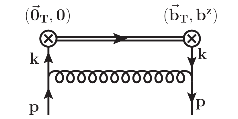
(a) Vertex diagram

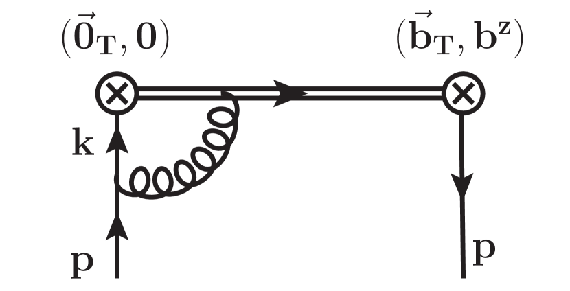
(b) Sail topology

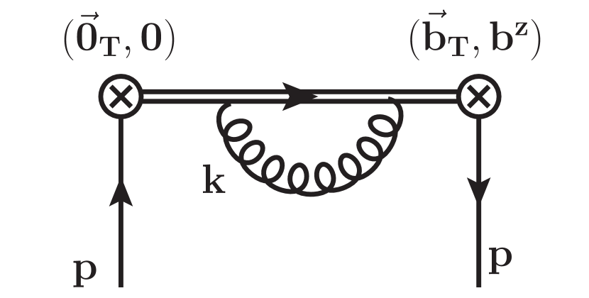
(c) Tadpole

Figure 4: One-loop diagrams contributing to the quasi-TMD beam function of eq. (15) in Feynman gauge. Mirror diagrams are not shown. The double line represents the Wilson line $W_{\sqsubset}$.

Vertex diagram

The vertex diagram in Fig. 4(a) gives Ebert:2019okf

$$\tilde{q}_{A}^{\tilde{\Gamma}\,(1)}(b,p) =\bigl{[}\bar{u}^{a}_{s}(p)u_{s}^{b}(p)\bigr{]}\frac{\alpha_{s}C_{F}}{4\pi}\Bigl{(}\gamma^{\mu}\gamma_{\alpha}\frac{\tilde{\Gamma}}{2}\gamma_{\beta}\gamma_{\mu}\Bigr{)}^{ab}\times\mathcal{I}_{v}^{\alpha\beta}(b,p)\,,$$ (45)

where the integral $\mathcal{I}_{v}^{\alpha\beta}$ is given by

$$\mathcal{I}_{v}^{\alpha\beta}(b,p) =-4\mathrm{i}\mu_{0}^{2\epsilon}\int\frac{\mathrm{d}^{d}k}{(2\pi)^{d-2}}\frac{k^{\alpha}k^{\beta}}{k^{4}(p-k)^{2}}\,e^{\mathrm{i}k\cdot b}\,.$$ (46)

To evaluate eq. (45), we first evaluate

$$\mathcal{I}_{v}(b^{2},p\cdot b) =-4\mathrm{i}\mu_{0}^{2\epsilon}\int\frac{\mathrm{d}^{d}k}{(2\pi)^{d-2}}\frac{e^{\mathrm{i}k\cdot b}}{k^{4}(p-k)^{2}}$$

$$=-\frac{1}{4}(\pi\mu_{0}^{2})^{\epsilon}\Gamma(-1-\epsilon)\frac{1+\mathrm{i}{p{\cdot}b}-e^{\mathrm{i}{p{\cdot}b}}}{({p{\cdot}b})^{2}}(-b^{2})^{1+\epsilon}\,,$$ (47)

which can be derived using standard techniques. Note that here we have made explicit that the integral can only depend on the two Lorentz invariants $b^{2}$ and ${p{\cdot}b}$, as $p^{2}=0$. From here, we note that

$$\mathcal{I}_{v}^{\alpha\beta}(b,p) =\left(\mathrm{i}\frac{\partial}{\partial b_{\alpha}}\right)\left(\mathrm{i}\frac{\partial}{\partial b_{\beta}}\right)\mathcal{I}_{v}(b^{2},{p{\cdot}b})$$

$$=-2g^{\alpha\beta}\frac{\partial\mathcal{I}_{v}}{\partial(b^{2})}-2(p^{\alpha}b^{\beta}+b^{\alpha}p^{\beta})\frac{\partial^{2}\mathcal{I}_{v}}{\partial(b^{2})\partial({p{\cdot}b})}-4b^{\alpha}b^{\beta}\frac{\partial^{2}\mathcal{I}_{v}}{\partial^{2}(b^{2})}-p^{\alpha}p^{\beta}\frac{\partial^{2}\mathcal{I}_{v}}{\partial^{2}({p{\cdot}b})}$$

$$=-2g_{\perp}^{\alpha\beta}\frac{\partial\mathcal{I}_{v}}{\partial(b^{2})}-4b^{\alpha}b^{\beta}\frac{\partial^{2}\mathcal{I}_{v}}{\partial^{2}(b^{2})}+\mathcal{O}(n^{\alpha},n^{\beta})\,.$$ (48)

When plugging eq. (3.3) into eq. (45), all terms with $n^{\alpha}$ or $n^{\beta}$ (or equivalently $p^{\alpha}$ or $p^{\beta}$) vanish due to $\not{n}u_{s}(p)=0$. This allows us to replace the full metric $g$ with the transverse metric $g_{\perp}$. It is now straightforward to evaluate eq. (45),

$$\tilde{q}_{A}^{\tilde{\Gamma}\,(1)}(b,p) =\bigl{[}\bar{u}^{a}_{s}(p)u_{s}^{b}(p)\bigr{]}\frac{\alpha_{s}C_{F}}{4\pi}\frac{\Gamma(-\epsilon)}{e^{\epsilon\gamma_{E}}}e^{\epsilon L_{b}}\Bigl{(}\gamma^{\mu}\gamma_{\alpha}\frac{\tilde{\Gamma}}{2}\gamma_{\beta}\gamma_{\mu}\Bigr{)}^{ab}$$

$$\quad\times\biggl{(}\frac{g_{\perp}^{\alpha\beta}}{2}+\epsilon\frac{b^{\alpha}b^{\beta}}{b^{2}}\biggr{)}\biggl{(}\frac{-b^{2}}{b_{T}^{2}}\biggr{)}^{\epsilon}\frac{1+\mathrm{i}{p{\cdot}b}-e^{\mathrm{i}{p{\cdot}b}}}{({p{\cdot}b})^{2}}\,.$$ (49)

We write Eq. (3.3) in terms of the Lorentz invariants $b^{2}$ and $p\cdot b$ so that it can be used to obtain both the TMDPDF and quasi-TMDPDF vertex diagrams. For the TMD, ${p{\cdot}b}=\frac{1}{2}p^{-}b^{+}$ and $b^{2}=b_{\perp}^{2}=-b_{T}^{2}$, whereas for the quasi-TMD we have ${p{\cdot}b}=-p^{z}b^{z}$ and $b^{2}=-b_{T}^{2}-(b^{z})^{2}$. In both cases, the required Fourier transform can be obtained from

$$\int\frac{\mathrm{d}({p{\cdot}b})}{2\pi}e^{-\mathrm{i}x{p{\cdot}b}}\,({p{\cdot}b})^{n}\,\frac{1+\mathrm{i}{p{\cdot}b}-e^{\mathrm{i}{p{\cdot}b}}}{({p{\cdot}b})^{2}}=\mathrm{i}^{n}\frac{\mathrm{d}^{n}}{\mathrm{d}^{n}x}(1-x)\theta(x)\theta(1-x)\,.$$ (50)

Note that the physical support $0\leq x\leq 1$ naturally arises in the integral in eq. (50). In the following we explicitly suppress the $\theta$ functions. When expanding eq. (3.3) in small $(b^{z}/b_{T})^{2}$, only the $n=0$ term contributes, yielding

$$\tilde{q}_{A}^{\tilde{\Gamma}\,(1)}(b,p) =\frac{1}{p^{z}}\bigl{[}\bar{u}^{a}_{s}(p)u_{s}^{b}(p)\bigr{]}\frac{\alpha_{s}C_{F}}{4\pi}\frac{\Gamma(-\epsilon)}{e^{\epsilon\gamma_{E}}}e^{\epsilon L_{b}}\Bigl{(}\gamma^{\mu}\gamma_{\alpha}\frac{\tilde{\Gamma}}{2}\gamma_{\beta}\gamma_{\mu}\Bigr{)}^{ab}(1-x)\left(\frac{g_{\perp}^{\alpha\beta}}{2}+\epsilon\frac{b_{\perp}^{\alpha}b_{\perp}^{\beta}}{b_{\perp}^{2}}\right)$$

$$=\frac{1}{p^{z}}\bigl{[}\bar{u}^{a}_{s}(p)u_{s}^{b}(p)\bigr{]}\frac{\alpha_{s}C_{F}}{4\pi}\Bigl{(}\gamma^{\mu}\gamma_{\alpha}\frac{\tilde{\Gamma}}{2}\gamma_{\beta}\gamma_{\mu}\Bigr{)}^{ab}$$

$$\quad\times(x-1)\left[\frac{g_{\perp}^{\alpha\beta}}{2}\left(\frac{1}{\epsilon}+L_{b}+1\right)-\left(\frac{g_{\perp}^{\alpha\beta}}{2}-\frac{b_{\perp}^{\alpha}b_{\perp}^{\beta}}{b_{\perp}^{2}}\right)\right]\,.$$ (51)

In the same fashion, we can obtain the vertex diagram of the TMDPDF, given above in eq. (3.2), where the $b_{T}/p^{-}$-suppressed term has $n=1$ and can be neglected at leading power. The close relationship between the two results is not surprising, as the two calculations only differ by the definition of $\tilde{\Gamma}$ and the choice of $b^{\mu}$.

Sail diagram

Next we consider the sail diagram in Fig. 4(b) and its mirror diagram. Extracting the overall Dirac structure, we write the sail diagram as

$$\tilde{q}_{B}^{\tilde{\Gamma}\,(1)}(b) =\frac{\alpha_{s}C_{F}}{2\pi}\Bigl{\{}\bigl{[}\bar{u}_{s}(p)\tilde{\Gamma}\gamma^{\rho}\gamma^{\mu}u_{s}(p)\bigr{]}\tilde{q}^{\tilde{\Gamma}\,(B1)}_{\mu\rho}(b^{\mu})+\bigl{[}\bar{u}_{s}(p)\gamma^{\mu}\gamma^{\rho}\tilde{\Gamma}u_{s}(p)\bigr{]}\tilde{q}^{\tilde{\Gamma}\,(B2)}_{\mu\rho}(b^{\mu})\Bigr{\}}\,,$$

$$\tilde{q}^{\tilde{\Gamma}\,(B1)}_{\mu\rho}(b) =-\frac{\mu_{0}^{2\epsilon}}{(2\pi)^{d-2}}\int\!\mathrm{d}^{d}k\int_{0}^{1}\mathrm{d}s\,\frac{\gamma^{\prime}(s)_{\mu}k_{\rho}}{k^{2}(p-k)^{2}}\,e^{\mathrm{i}p\cdot b-\mathrm{i}(p-k)\cdot\gamma(s)}\,,$$

$$\tilde{q}^{\tilde{\Gamma}\,(B2)}_{\mu\rho}(b) =-\frac{\mu_{0}^{2\epsilon}}{(2\pi)^{d-2}}\int\!\mathrm{d}^{d}k\int_{0}^{1}\mathrm{d}s\,\frac{\gamma^{\prime}(s)_{\mu}k_{\rho}}{k^{2}(p-k)^{2}}\,e^{\mathrm{i}k\cdot b+\mathrm{i}(p-k)\cdot\gamma(s)}\,,$$ (52)

where $\gamma(s)$ is the path of the Wilson lines. To make a connection to the calculation presented in Ref. Ebert:2019okf , we work with the path given in eq. (15) and illustrated in the left panel of Fig. 2, but we stress that in the limit $L\gg b_{T}$ this path is equivalent to the one in eq. (2.2).

We insert $\tilde{q}^{\tilde{\Gamma}\,(B1)}_{\mu\rho}$ into $\tilde{q}_{B}^{\tilde{\Gamma}\,(1)}$ and simplify the result using the on-shell condition $\not{n}u_{s}(p)=0$, giving

$$\not{k}\not{\gamma}^{\prime}u_{s}(p) =\Bigl{[}k^{-}\frac{\not{n}}{2}+k^{+}\frac{\not{{\bar{n}}}}{2}+\not{k}_{\perp}\Bigr{]}\Bigl{[}\gamma^{\prime-}\frac{\not{n}}{2}+\gamma^{\prime+}\frac{\not{{\bar{n}}}}{2}+\not{\gamma}^{\prime}_{\perp}\Bigr{]}u_{s}(p)$$

$$=\Bigl{[}k^{-}\gamma^{\prime+}+\frac{\not{{\bar{n}}}}{2}\bigl{(}k^{+}\not{\gamma}^{\prime}_{\perp}-\not{k}_{\perp}\gamma^{\prime+}\bigr{)}+\not{k}_{\perp}\not{\gamma}^{\prime}_{\perp}\Bigr{]}u_{s}(p)\,.$$ (53)

Here, we suppress the argument of $\gamma^{\prime}\equiv\gamma^{\prime}(s)$ and employ lightcone coordinates to make the on-shell condition manifest, noting that in practice $\gamma^{\prime+}=-\gamma^{\prime z}$. The calculation for $\tilde{q}^{\tilde{\Gamma}\,(B2)}_{\mu\rho}(b^{\mu})$ works similarly.

In eq. (3.3), the contributions with $\not{\gamma}_{\perp}^{\prime}$ arise from the transverse gauge links. In particular, evaluation of the line integrals in eq. (3.3) gives

$$\int_{0}^{1}\!\!\mathrm{d}s\,\gamma^{\prime}(s)_{\mu}e^{\mathrm{i}q\cdot\gamma(s)} =\mathrm{i}\hat{z}_{\mu}\frac{e^{-\mathrm{i}q^{z}L}-1}{q^{z}}+\mathrm{i}b_{\perp\mu}e^{-\mathrm{i}q^{z}L}\frac{e^{-\mathrm{i}\vec{b}_{T}\cdot\vec{q}_{T}}-1}{\vec{b}_{T}\cdot\vec{q}_{T}}+\mathrm{i}\hat{z}_{\mu}\frac{e^{-\mathrm{i}b^{z}q^{z}}-e^{-\mathrm{i}q^{z}L}}{q^{z}}e^{-\mathrm{i}\vec{b}_{T}\cdot\vec{q}_{T}}\,.$$ (54)

The perpendicular contribution contains a pure phase $e^{-\mathrm{i}q^{z}L}$, which oscillates quickly in the limit $L,p^{z}\to\infty$ and makes this term neglectable. This is analogous to how transverse gauge links do not contribute in nonsingular gauges. Thus, we can approximate eq. (3.3):

$$\not{k}\not{\gamma}^{\prime}u_{s}(p) =\bigl{(}k^{-}-\not{k}_{\perp}\bigr{)}\gamma^{\prime+}u_{s}(p)+\mathcal{O}\Bigl{(}\frac{1}{p^{z}L}\Bigr{)}\,.$$ (55)

After Fourier-transforming eq. (3.3) with respect to $b^{z}$, $\tilde{q}_{B}^{\tilde{\Gamma}\,(1)}$ only depends on $p^{-}$ and $b_{\perp}$. Thus, the contributions from the Dirac structures $k^{-}$ and $\not{k}_{\perp}$ in eq. (55) parametrically behave as $p^{-}$ and $\not{b}_{\perp}/b_{T}^{2}$, respectively. The latter is suppressed in the limit $b_{T}p^{z}\gg 1$, similar to the subleading-twist terms in the physical TMDPDF, cf. eq. (3.2). We can thus further expand

$$\not{k}\not{\gamma}^{\prime}u_{s}(p) =k^{-}\gamma^{\prime+}u_{s}(p)+\mathcal{O}\Bigl{(}\frac{1}{p^{z}L},\frac{1}{b_{T}p^{z}}\Bigr{)}\,.$$ (56)

Overall, in the physical limit eq. (3.3) reduces to the tree-level Dirac structure, leaving us free to write

$$\tilde{q}_{B}^{\tilde{\Gamma}\,(1)}(x,\vec{b}_{T}) =\frac{1}{p^{z}}\Bigl{[}\bar{u}_{s}(p)\frac{\tilde{\Gamma}}{2}u_{s}(p)\Bigr{]}\frac{\alpha_{s}C_{F}}{4\pi}\,\tilde{q}_{B}(x,\vec{b}_{T})\,,$$ (57)

where $\tilde{q}_{B}(x,\vec{b}_{T})$ is the one-loop coefficient of the unpolarized quasi beam function, i.e.,

$$\frac{1}{2}\sum_{s}\tilde{q}_{B}^{\gamma^{z}\,(1)}(x,\vec{b}_{T})=\frac{\alpha_{s}C_{F}}{4\pi}\,\tilde{q}_{B}(x,\vec{b}_{T})\,.$$ (58)

We can also read off from the result in Ref. Ebert:2019okf that

$$\tilde{q}_{B}(x,\vec{b}_{T}) =\Bigl{(}\frac{1}{\epsilon}+L_{b}\Bigr{)}\Bigl{[}-4\mathcal{L}_{0}(1-x)-2\delta(1-x)L_{p^{z}}+4\Bigr{]}$$

$$\quad+\delta(1-x)\Bigl{(}-\frac{2}{\epsilon}+\frac{2}{\epsilon}L_{p^{z}}-L_{b}^{2}-L_{p^{z}}^{2}+2L_{p^{z}}-4\Bigr{)}\,,$$ (59)

where $L_{p^{z}}=\ln[(2p^{z}/\mu)^{2}]$. The plus distribution ${\cal L}_{0}(1-x)$ implicitly only has support for $x\in[0,1]$. Note that the pole in the first line in eq. (3.3) has an IR origin, and thus must agree with the corresponding IR pole in the TMDPDF so that the IR divergences cancel each other out in the matching. By comparing to eq. (3.2), it is easy to see that this holds upon identifying $\zeta=(2p^{z})^{2}$.

Tadpole diagram

The Wilson line self-energy in Fig. 4(c) is given by

$$\tilde{q}_{C}^{\tilde{\Gamma}\,(1)}(x,\vec{b}_{T}) =\frac{\mathrm{i}}{p^{z}}\Bigl{[}\bar{u}_{s}(p)\frac{\tilde{\Gamma}}{2}u_{s}(p)\Bigr{]}\frac{\alpha_{s}C_{F}}{2\pi}\frac{\mu_{0}^{2\epsilon}}{(2\pi)^{d-2}}\int_{0}^{1}\mathrm{d}s\,\mathrm{d}t\,[\gamma^{\prime}(s)\cdot\gamma^{\prime}(t)]\int\!\mathrm{d}^{d}k\frac{e^{\mathrm{i}k\cdot[\gamma(s)-\gamma(t)]}}{k^{2}+\mathrm{i}0}$$

$$\equiv\frac{1}{p^{z}}\Bigl{[}\bar{u}_{s}(p)\frac{\tilde{\Gamma}}{2}u_{s}(p)\Bigr{]}\frac{\alpha_{s}C_{F}}{4\pi}\,\tilde{q}_{C}(x,\vec{b}_{T})\,.$$ (60)

Since the Wilson line vertices do not have a Dirac structure, the tadpole contribution is trivially proportional to the tree level Dirac structure. In eq. (3.3), $\tilde{q}_{C}(x,\vec{b}_{T})$ is the coefficient of the tadpole diagram of the unpolarized quasi beam function because

$$\frac{1}{2}\sum_{s}\tilde{q}_{C}^{\gamma^{z}\,(1)}(x,\vec{b}_{T})=\frac{\alpha_{s}C_{F}}{4\pi}\,\tilde{q}_{C}(x,\vec{b}_{T})\,.$$ (61)

From Ref. Ebert:2019okf we can read off

$$\tilde{q}_{C}(x,\vec{b}_{T}) =\delta(1-x)\biggl{[}\frac{6}{\epsilon}+6L_{b}+4+\frac{4\pi L}{b_{T}}+\mathcal{O}(\epsilon)\biggr{]}\,,$$ (62)

up to corrections suppressed in the $P^{z}b_{T}\gg 1$ and $L/b_{T}\gg 1$ limits. We remark upon the explicit $L/b_{T}$ divergence in eq. (62), which must be canceled by the soft factor in a manner analogous to the cancellation of rapidity divergences that appears in the TMD case (see Ref. Ebert:2019okf ).

Combined result

The sum of the results for the vertex, sail and tadpole diagrams gives the bare quasi beam function at one loop,

$$\tilde{B}_{q/h_{S}}^{[\tilde{\Gamma}]}(x,\vec{b}_{T},\epsilon,p^{z}) =\frac{1}{p^{z}}\biggl{[}\bar{u}_{s}(p)\frac{\tilde{\Gamma}}{2}u_{s}(p)\biggr{]}\Bigl{\{}\delta(1-x)+\frac{\alpha_{s}C_{F}}{4\pi}\bigl{[}\tilde{B}_{b}^{(1)}+\tilde{R}_{B}^{(1)}\delta(1-x)\bigr{]}\Bigr{\}}$$

$$\quad+\frac{\alpha_{s}C_{F}}{4\pi}\frac{1}{p^{z}}\Bigl{[}\bar{u}_{s}(p)\gamma^{\mu}\gamma_{\alpha}\frac{\tilde{\Gamma}}{2}\gamma_{\beta}\gamma_{\mu}u_{s}(p)\Bigr{]}\biggl{[}\tilde{B}_{a1}^{(1)}\frac{g_{\perp}^{\alpha\beta}}{2}+\tilde{B}_{a2}^{(1)}\Bigl{(}\frac{g_{\perp}^{\alpha\beta}}{2}-\frac{b_{\perp}^{\alpha}b_{\perp}^{\beta}}{b_{\perp}^{2}}\Bigr{)}\biggr{]}$$

$$\quad+\mathcal{O}(\alpha_{s}^{2})\,.$$ (63)

The coefficient functions, whose arguments we keep implicit, are given by

$$\tilde{B}_{b}^{(1)} =\Bigl{(}\frac{1}{\epsilon_{\rm IR}}+L_{b}\Bigr{)}[-2P_{qq}(x)+2(1-x)]$$

$$\quad+\delta(1-x)\Bigl{[}\frac{7}{\epsilon}-(L_{b}+L_{P^{z}})^{2}+2L_{P^{z}}+9L_{b}\Bigr{]}+\mathcal{O}(\epsilon)\,,$$

$$\tilde{B}_{a1}^{(1)} =-(1-x)\Bigl{(}\frac{1}{\epsilon_{\rm IR}}+L_{b}+1\Bigr{)}+\mathcal{O}(\epsilon)\,,$$

$$\tilde{B}_{a2}^{(1)} =(1-x)+\mathcal{O}(\epsilon)\,.$$ (64)

Note that we separated out the divergent term into $\tilde{R}_{B}^{(1)}=4\pi L/b_{T}$ and made the origin of all poles as either IR or UV explicit. Evaluating eq. (3.3) for the three Dirac structures in eq. (17), we obtain the UV-renormalized quasi beam functions:

$$\tilde{B}_{q/h_{S}}^{[\gamma^{\lambda}]}(x,\vec{b}_{T},\mu,p^{z}) =\delta(1-x)\Bigl{\{}1+\frac{\alpha_{s}C_{F}}{4\pi}\Bigl{[}-(L_{b}+L_{P^{z}})^{2}+2L_{P^{z}}+9L_{b}+\tilde{R}_{B}^{(1)}\Bigr{]}\Bigr{\}}$$

$$\quad+\frac{\alpha_{s}C_{F}}{4\pi}\Bigl{[}-2\Bigl{(}\frac{1}{\epsilon_{\rm IR}}+L_{b}\Bigr{)}P_{qq}(x)+2(1-x)\Bigr{]}+\mathcal{O}(\alpha_{s}^{2})\,,$$

$$\tilde{B}_{q/h_{S}}^{[\gamma^{\lambda}\gamma]}(x,\vec{b}_{T},\mu,p^{z}) =\Lambda\tilde{B}_{q/h_{S}}^{[\gamma^{\lambda}]}(x,\vec{b}_{T},\mu,p^{z})+\mathcal{O}(\alpha_{s}^{2})\,,$$

$$\tilde{B}_{q/h_{S}}^{[\mathrm{i}\sigma^{\alpha\lambda}\gamma_{5}]}(x,\vec{b}_{T},\mu,p^{z}) =s_{\perp}^{\alpha}\delta(1-x)\Bigl{\{}1+\frac{\alpha_{s}C_{F}}{4\pi}\Bigl{[}-(L_{b}+L_{P^{z}})^{2}+2L_{P^{z}}+9L_{b}+\tilde{R}_{B}^{(1)}\Bigr{]}\Bigr{\}}$$

$$\quad+s_{\perp}^{\alpha}\frac{\alpha_{s}C_{F}}{4\pi}\Bigl{[}-2\Bigl{(}\frac{1}{\epsilon_{\rm IR}}+L_{b}\Bigr{)}P^{T}_{qq}(x)\Bigr{]}+\mathcal{O}(\alpha_{s}^{2})\,.$$ (65)

Similar to eq. (3.2), the $\delta(1-x)$ terms in eq. (3.3) agree for all choices of $\tilde{\Gamma}$ as they arise entirely from the sail diagrams, which are proportional to the tree-level Dirac structure. We have explicitly validated this in appendix B.2. The differences result entirely from the vertex diagram, which is absent for the transverse structure, see also appendix B.1. We also note that all results are independent of the choice $\lambda=t$ or $\lambda=z$.

3.4 One-loop matching

By comparing the results in eqs. (3.2) and (3.3) and noting that the unspecified quasi soft factor is spin independent, we see that the ratios of quasi-TMDPDFs and TMDPDFs agree for the unpolarized, helicity and transversity structures,

$$\frac{\tilde{f}_{1}(x,b_{T},\mu,P^{z})}{f_{1}(x,b_{T},\mu,\zeta)} =\frac{\tilde{g}_{1L}(x,b_{T},\mu,P^{z})}{g_{1L}(x,b_{T},\mu,\zeta)}=\frac{\tilde{h}_{1}(x,b_{T},\mu,P^{z})}{h_{1}(x,b_{T},\mu,\zeta)}\,.$$ (66)

From eq. (24), it follows that the short-distance matching kernel is identical for these functions. Using the result from Ref. Ebert:2019okf , we thus obtain

$$C_{\rm ns}^{f_{1}}(\mu,xP^{z}) =C_{\rm ns}^{g_{1L}}(\mu,xP^{z})=C_{\rm ns}^{h_{1}}(\mu,xP^{z})$$

$$=1+\frac{\alpha_{s}C_{F}}{4\pi}\biggl{[}-\ln^{2}\frac{(2xP^{z})^{2}}{\mu^{2}}+2\ln\frac{(2xP^{z})^{2}}{\mu^{2}}-4+\frac{\pi^{2}}{6}\biggr{]}+\mathcal{O}(\alpha_{s}^{2})\,.$$ (67)

This is the main result of our analysis. We discuss a reason for this observed universality in Sec. 3.5, where we also discuss the extension of this observation to higher orders.

It is interesting to note that the one-loop results of the both the TMDPDF and the quasi beam functions, see eqs. (3.2) and (3.3), consist of universal kinematic structures, whereas the dependence on $\Gamma$ and $\tilde{\Gamma}$ only arises through the Dirac traces. The Dirac traces are identical for each choice for $\Gamma$/$\tilde{\Gamma}$, and thus the spin independence of the ratios of quasi-TMDs to TMDs can be traced back to the universal kinematic structure of the one-loop diagrams. Based on this observation, we present more general arguments for the spin independence of the matching kernel in Sec. 3.5. In addition, since the tree-level Dirac structures are all normalized, only the Dirac trace arising from the vertex diagram can lead to differences between different spin-dependent quasi-TMDs, or between different spin-dependent TMDs, respectively. Since the vertex diagram only encodes collinear interactions between the external quarks, which are not affected by the different Wilson line geometries, it obeys the simple boost picture underlying LaMET and does not affect the matching. In contrast, the sail and tadpole diagrams, as well as the soft subtraction, resolve the Wilson line structure; thus, they induce a nontrivial matching.

The $f_{1T}^{\perp}$, $g_{1T}$, $h_{1L}^{\perp}$, and $h_{1}^{\perp}$ distributions, which are proportional to $b_{\perp}^{\alpha}/b_{T}$, cannot be constrained by the setup used for our calculation. The chosen on-shell quark state for the one-loop calculation has no overlap with the corresponding (quasi-)TMDPDF operators. The analysis for these functions is beyond the scope of the present work.

A special case is the pretzelosity distribution $h_{1T}^{\perp}$, which is proportional to $g_{\perp}^{\alpha\beta}/2-b_{\perp}^{\alpha}b_{\perp}^{\beta}/b_{\perp}^{2}$, cf. eq. (2.1). From eqs. (3.2) and (3.3), it is clear that this contribution arises first at one loop from the vertex diagram for both the quasi and non-quasi TMDs. It does not contain any divergences or logarithms and in both cases is simply proportional to

$$\Bigl{[}\bar{u}_{s}(p)\gamma^{\mu}\gamma_{\alpha}\frac{\mathrm{i}\sigma^{\rho\lambda}\gamma_{5}}{2}\gamma_{\beta}\gamma_{\mu}u_{s}(p)\Bigr{]} =p^{\lambda}(d-4)\bigl{(}s^{\rho}g_{\alpha\beta}-s_{\beta}g^{\rho}_{\alpha}-s_{\alpha}g^{\rho}_{\beta}\Bigr{)}\,.$$ (68)

Here, we use naive dimensional regularization with anticommuting $\gamma^{5}$ and $p\cdot s=0$, and furthermore that $\alpha$, $\beta$ and $\rho$ are transverse indices, while $\lambda$ is not. Eq. (68) implies that pretzelosity formally contributes at NLO but vanishes in dimensional regularization for $d=4$, so that the $\overline{\rm MS}$-renormalized pretzelosity quasi-TMD (and TMD) is zero at this order. In fact, for matching using massless quark states, Refs. Gutierrez-Reyes:2017glx ; Gutierrez-Reyes:2018iod observe that the pretzelosity matrix elements vanish through two loops, and Ref. Chai:2018mwx argues that this holds to all orders in perturbation theory. Recall that the requirement to carry out a valid matching calculation is that the chosen states have overlap with the operators being considered, which is not achieved with the above choices for pretzelosity. Interestingly, we can consider matching using massless quark states with $d\neq 4$. In this case the $(d-4)$ prefactor occurs for both the quasi-TMD and TMD and cancels in their ratio, so we find

$$\tilde{h}_{1T}^{\perp}(x,b_{T},\mu,P^{z})=h_{1T}^{\perp}\bigl{(}x,b_{T},\mu,\zeta=(2xP^{z})^{2}\bigr{)}\times\bigl{[}1+\mathcal{O}(\alpha_{s})]\,.$$ (69)

In this matching relation the Wilson coefficient is only obtained at tree level, since the overlap matrix elements themselves start at one-loop. To obtain the one-loop matching kernel for the quasi-pretzelosity in this fashion would require a two-loop calculation, which is beyond our goals here. However, the line of reasoning in Sec. 3.5 suggests that $C_{\rm ns}^{h_{1T}^{\perp}}(\mu,xP^{z})$ will also be universal with the same value as in eq. (3.4). A calculation of the ratio $\tilde{h}_{1T}^{\perp}/\tilde{f}_{1}$ would determine the size of the pretzelosity distribution relative to the unpolarized TMDPDF, which is an interesting target for lattice QCD.

3.5 Generalization of matching to all orders

It is interesting to ask whether the observed spin independence of the one-loop matching kernels obtained in eq. (3.4) will continue to higher loop orders. In this section we outline an argument that this universality will continue to hold to all orders, without providing sufficient detail to call it a complete proof.

In the one-loop matching calculation we observed that it was the graphs associated to attachments to the Wilson lines that led to the mismatch between quasi-TMD and TMD contributions, and hence to a nonzero result for the matching coefficient. At leading order in power counting, these Wilson line graphs could not modify the spin structure of the initial operator. This is reminiscent of the spin universality of Soft Collinear Effective Theory (SCET) diagrams for heavy-to-light and back-to-back light-to-light currents Bauer:2000yr ; Bauer:2002nz ; SCETlecture , which arise from the spin universality of Wilson line and self-energy diagrams.

Consider the generic beam function and quasi beam function correlators using quark fields with open Dirac spin indices $i$ and $j$,

$$B_{ij,q/h_{S}}(b^{+},\vec{b}_{T},a,\tau,P^{-}) =\Bigl{<}h(P)\Bigr{|}\Bigl{[}\bar{q}_{i}(b^{\mu})W_{\sqsubset}(b^{\mu},0)q_{j}(0)\Bigr{]}_{\tau,a}\Bigl{|}h(P)\Bigr{>}\,,$$

$$\tilde{B}_{ij,q/h_{S}}(b^{z},\vec{b}_{T},a,L,P^{z}) =\Bigl{<}h(P)\Bigr{|}\Bigl{[}\bar{q}_{i}(b^{\mu})\widetilde{W}_{\sqsubset}(b^{\mu},0;L)q_{j}(0)\Bigr{]}_{a}\Bigl{|}h(P)\Bigr{>}\,.$$ (70)

The paths for the Wilson lines are shown in Figs. 1 and 2, respectively. We notice that the vertices on the four corners of the Wilson lines are separated by long distances, either $\sim b_{T}$ or $\sim L$ for $\tilde{B}_{ij,q/h_{S}}$, or $\sim b_{T}$ or $\infty$ for $B_{ij,q/h_{S}}$. These straight Wilson lines can be rewritten in terms of local operators by the now standard method of introducing scalar auxiliary fields $X_{v}$ for a line along the four-vector $v^{\mu}$ Korchemsky:1987wg . For simplicity one can introduce three different auxiliary fields whose direction is along each straight Wilson line segment in Fig. 2, and another three auxiliary fields for the segments in Fig. 1. In this case both the quasi beam function and beam function calculations become matrix elements of a product of four local current operators whose spacetime arguments situate them at each of the corresponding four corners. We can refer to them as the current operators, such as $X_{T}^{\dagger}X_{n}$ and $X_{n}^{\dagger}q_{i}$, and quasi-current operators, such as $X_{T}^{\dagger}X_{\hat{z}}$ and $X_{\hat{z}}^{\dagger}q_{i}$. With this setup, two out of the four current operators (or quasi-current operators) have open spin indices ($i$ or $j$).

When we carry out the matching in this setup we are matching one nonlocal product of operators onto another nonlocal product of operators; therefore one expects that the short-distance contribution is isolated to a matching coefficient $C$ at each of the currents when taking the boosted limit $X_{\hat{z}}^{\dagger}q_{i}\to CX_{n}^{\dagger}q_{i}$. This type of matching is like what occurs in SCET when matching a full theory current in boosted kinematics onto boosted $n$-collinear fields. Due to the spin universality of the scalar auxiliary fields, no spin dependence will be introduced for the resulting short-distance matching coefficients $C$ at any order in $\alpha_{s}$. These arguments clearly must be extended to account for rapidity divergences that appear in the light-like limit, as well as non-trivial quasi soft and soft functions, but these are spin-independent and hence will not modify the spin universality of the matching coefficient. These rapidity factors and soft functions cancel out in ratios.

In the situation with infinite staple lengths, an analysis of this type that uses auxiliary fields was carried out recently in Ref. Vladimirov:2020ofp , from which we have drawn inspiration. The goal in that work was to derive the quasi-TMDPDF to TMDPDF matching relation. Ref. Vladimirov:2020ofp uses SCET in a somewhat different fashion than what we envisioned above because they consider the analogy of the quasi-TMDPDF with a TMD hadronic tensor, and perform a match up which simultaneously yields $n$-collinear, ${\bar{n}}$-collinear, and soft fields. It is known that a quasi soft function is needed as part of the definition of the quasi-TMDPDF in order to properly carry out the quasi-TMDPDF to TMDPDF matching Ji:2014hxa ; Ji:2018hvs ; Ebert:2019okf , and it is so far not clear how the quasi soft function is treated by the analysis in Ref. Vladimirov:2020ofp , which is also the case for our outline above.

4 Applications

We now discuss applications of our main finding in eq. (3.4). We find that the ratios of spin-dependent TMDs and the unpolarized TMD can be directly obtained from those of the quasi-TMDs, i.e.

$$\frac{g_{1L}(x,b_{T},\mu,\zeta)}{f_{1}(x,b_{T},\mu,\zeta)} =\frac{\tilde{g}_{1L}(x,b_{T},\mu,P^{z})}{\tilde{f}_{1}(x,b_{T},\mu,P^{z})}\,,$$

$$\frac{h_{1}(x,b_{T},\mu,\zeta)}{f_{1}(x,b_{T},\mu,\zeta)} =\frac{\tilde{h}_{1}(x,b_{T},\mu,P^{z})}{\tilde{f}_{1}(x,b_{T},\mu,P^{z})}\,,$$

$$\frac{h_{1T}^{\perp}(x,b_{T},\mu,\zeta)}{f_{1}(x,b_{T},\mu,\zeta)} =\frac{\tilde{h}_{1T}^{\perp}(x,b_{T},\mu,P^{z})}{\tilde{f}_{1}(x,b_{T},\mu,P^{z})}\,.$$ (71)

In these ratios the matching coefficients drop out along with the nonperturbative soft contributions in the function $g_{q}^{S}$ and the Collins-Soper evolution factor. The anomalous dimensions for the $\mu$- and Collins-Soper evolutions are the same for the TMDs here, so the ratios on both the left- and the right-hand sides are only dependent on $x$ and $b_{T}$. These relations have power corrections that are suppressed by $1/(P^{z}b_{T})$, so one can calculate the ratios on the r.h.s. in lattice QCD with different hadron momenta and interpolate to $P^{z}\to\infty$ to obtain the final result.

In addition, we can consider the ratios of the $x$-integrated TMDs which were studied in a different formalism based on exploiting Lorentz invariance in Refs. Musch:2010ka ; Musch:2011er ; Engelhardt:2015xja ; Yoon:2016dyh ; Yoon:2017qzo . According to eq. (2.2),

$$\int_{-1}^{1}\!\mathrm{d}x\,\tilde{f}_{q/h_{S}}^{[\tilde{\Gamma}]}(x,\vec{b}_{T},\mu,P^{z}) =\tilde{Z}^{\prime}_{q}(0,\mu,\tilde{\mu})\tilde{Z}_{\rm uv}^{q}(0,\tilde{\mu},a)\tilde{\Delta}_{S}^{q}(b_{T},a,L)\tilde{B}_{q/h_{S}}^{[\tilde{\Gamma}]}(b^{z}=0,\vec{b}_{T},a,L,P^{z})\,,$$ (72)

where $\tilde{B}_{q/h_{S}}^{[\tilde{\Gamma}]}(b^{z}=0,\vec{b}_{T},a,L,P^{z})$ is the bare quasi beam function. The r.h.s. of eq. (72) is finite, so the $x$-integration of the quasi-TMD is convergent. According to eq. (2.3), we have

$$\frac{\int\!\mathrm{d}x\,\tilde{F}_{{\rm ns}/h_{S}}(x,b_{T},\mu,P^{z})}{\int\!\mathrm{d}x\,\tilde{f}_{1}(x,b_{T},\mu,P^{z})} =\frac{\tilde{B}_{{\rm ns}/h_{S}}(0,b_{T},a,L,P^{z})}{\tilde{B}_{\rm ns}(0,b_{T},a,L,P^{z})}$$

$$=\frac{\int\!\mathrm{d}x\,C_{{\rm ns}}\bigl{(}\mu,xP^{z}\bigr{)}\>F_{{\rm ns}/h_{S}}\big{(}x,b_{T},\mu,\zeta=(2xP^{z})^{2}\big{)}}{\int\!\mathrm{d}x\,C_{{\rm ns}}\bigl{(}\mu,xP^{z}\bigr{)}\>f_{1}\big{(}x,b_{T},\mu,\zeta=(2xP^{z})^{2}\big{)}}\,.$$ (73)

Thus we see that this ratio of $x$-integrated quasi-TMDPDF is not directly related to the ratio of $x$-integrated TMDs $F_{{\rm ns}/h_{S}}$ and $f_{1}$ in the formalism used here.

5 Conclusion

This paper constructs spin-dependent quasi-TMDPDFs that have a straightforward implementation in lattice calculations. We study the relationship between these spin-dependent quasi-TMDPDFs and their corresponding TMDPDFs at next-to-leading order. The nonperturbative soft factor and Collins-Soper evolution cancel in the ratio of polarized and unpolarized quasi-TMDs, and in the ratio of the corresponding TMDs. This leads to a simple relationship between the quasi-TMD and TMD ratios involving only a perturbative matching kernel, see eq. (24). We calculate these kernels explicitly at one-loop in Sec. 3.

At one-loop order in massless perturbation theory, we have access to the unpolarized ($f_{1}$), helicity ($g_{1L}$), and transversity ($h_{1}$) structures, which remarkably have the same perturbative kernel as the unpolarized case $C_{{\rm ns}}^{f_{1}}=C_{\rm ns}^{g_{1L}}=C_{\rm ns}^{h_{1}}$. A key reason for this simple result is that all diagrams with nontrivial $x$ dependence must cancel (up to power corrections) between the perturbative results of quasi-TMDs and TMDs to give rise to an $x$-independent matching, as required by consistency Ebert:2019okf . The remaining diagrams only contain the tree-level Dirac structure (which cancels out in suitable ratios) because the kinematic structures of all diagrams involving Wilson lines are independent of spin, up to power corrections.

An interesting feature of the pretzelosity is that its matrix element first appears at one-loop order, but vanishes in dimensional regularization when $d-4=-2\epsilon=0$. For $\epsilon\neq 0$ we can carry out matching between the pretzelosity and quasi-pretzelosity, and they again satisfy the same relation as the aforementioned spin structures, yielding a simple matching relation at tree-level. The remaining spin structures, namely the Sivers function ($f_{1T}^{\perp}$), Boer-Mulders function ($h_{1}^{\perp}$) and worm-gear functions ($g_{1T}$, $h_{1L}^{\perp}$), vanish in massless perturbation theory and are thus beyond the scope of this paper.

We also consider a definition of the quasi beam function with a staple-shaped Wilson line whose length remains constant under a Fourier transform. This avoids the necessity of a $b^{z}$-dependent counterterm to cancel Wilson line self energies, and thus simplifies one aspect of lattice calculations of quasi-TMDPDF ratios. We discuss implications of this definition for the determination of the Collins-Soper kernel in appendix A.

Finally, in Sec. 3.5 we outline a procedure for generalizing the universality of the spin-dependent matching coefficients to all orders in perturbation theory. We intend to carry out a more detailed analysis of this procedure in future work, as well as to obtain matching relations for the Sivers, Boer-Mulders, and worm-gear functions.

Appendix A Alternative construction of the quasi beam function

In Sec. 2.2, we mentioned that the definition of the quasi beam function in eq. (2.2) has the nice feature that its renormalization factor is independent of $b^{z}$, which drops out in the ratios of quasi-TMDPDFs, simplifying the lattice calculations. In this appendix we contrast the definitions in eq. (15) and eq. (2.2) at a more technical level.

Take the Collins-Soper evolution kernel as an example. According to Refs. Ebert:2018gzl ; Ebert:2019tvc ; Shanahan:2020zxr , we can extract the nonperturbative Collins-Soper evolution kernel for TMDPDFs from the ratio of quasi-TMDPDFs at different hadron momenta for the definition in eq. (15),

$$\gamma^{q}_{\zeta}(\mu,b_{T})=\frac{1}{\ln(P^{z}_{1}/P^{z}_{2})}$$ (74)

$$\times\ln\frac{C_{\rm ns}(\mu,xP_{2}^{z})\,\int\!\mathrm{d}b^{z}\,e^{ib^{z}xP_{1}^{z}}\,\tilde{Z}_{q}^{\prime}(b^{z},\mu,\tilde{\mu})\,\tilde{Z}_{\rm uv}^{q}(b^{z},\tilde{\mu},a)\,{\tilde{R}}_{B}(b_{T},\tilde{\mu},a,L)\,\tilde{B}_{\rm ns}(b^{z},\vec{b}_{T},a,P_{1}^{z},L)}{C_{\rm ns}(\mu,xP_{1}^{z})\,\int\!\mathrm{d}b^{z}\,e^{ib^{z}xP_{2}^{z}}\,\tilde{Z}_{q}^{\prime}(b^{z},\mu,\tilde{\mu})\,\tilde{Z}_{\rm uv}^{q}(b^{z},\tilde{\mu},a)\,{\tilde{R}}_{B}(b_{T},\tilde{\mu},a,L)\,\tilde{B}_{\rm ns}(b^{z},\vec{b}_{T},a,P_{2}^{z},L)}\,,$$

where the quasi soft factor $\tilde{\Delta}_{S}^{q}$ cancels out, and the $b^{z}$-independent factor $\tilde{R}_{B}$ is constructed such that it exactly removes all divergences that would normally be canceled by $\tilde{\Delta}_{S}^{q}(b_{T},a,L)$ Ebert:2019tvc , i.e. all power-law divergences not yet absorbed by $\tilde{Z}_{\rm uv}^{q}(b^{z},\tilde{\mu},a)$. In this way, we can take the $L\to\infty$ and $a\to 0$ limits before forming the ratio.

If we instead use the alternative definition in eq. (2.2), both $\tilde{Z}_{\rm uv}^{q}(\tilde{\mu},a)$ and $\tilde{Z}_{q}^{\prime}(\mu,\tilde{\mu})$ also drop out in the ratios of the quasi-TMDPDFs. Therefore, if one loosens the requirement that the $L\to\infty$ and $a\to 0$ limits be taken first, the Collins-Soper kernel can be obtained from the ratio of bare quasi beam functions on the lattice,

$$\gamma^{q}_{\zeta}(\mu,b_{T}) =\frac{1}{\ln(P^{z}_{1}/P^{z}_{2})}\ln\left[\lim_{\begin{subarray}{c}L\to\infty\\ a\to 0\end{subarray}}\frac{C_{\rm ns}(\mu,xP_{2}^{z})\,\int\!\mathrm{d}b^{z}\,e^{ib^{z}xP_{1}^{z}}\,\tilde{B}_{{\rm ns}}(b^{z},\vec{b}_{T},a,P_{1}^{z},L)}{C_{\rm ns}(\mu,xP_{1}^{z})\,\int\!\mathrm{d}b^{z}\,e^{ib^{z}xP_{2}^{z}}\,\tilde{B}_{{\rm ns}}(b^{z},\vec{b}_{T},a,P_{2}^{z},L)}\right]\,.$$ (75)

If one wants to take the $L\to\infty$ and $a\to 0$ limits before forming the ratio, then $\tilde{Z}_{\rm uv}^{q}(\tilde{\mu},a)$ and $\tilde{Z}_{q}^{\prime}(\mu,\tilde{\mu})$ can be included and chosen as $\tilde{Z}_{\rm uv}^{q}(b^{z}=0,\tilde{\mu},a)$ and $\tilde{Z}_{q}^{\prime}(b^{z}=0,\mu,\tilde{\mu})$ which have already been studied in the RI/MOM scheme for the quasi beam function in eq. (14) Constantinou:2019vyb ; Ebert:2019tvc ; Shanahan:2019zcq . Moreover, to exploit the $b^{z}$-independence, we might as well divide the bare quasi beam functions by $\tilde{B}_{{\rm ns}}(b^{z}=0,\vec{b}_{T},a,P^{z},L)$, i.e.,

$$\gamma^{q}_{\zeta}(\mu,b_{T})=\frac{1}{\ln(P^{z}_{1}/P^{z}_{2})}$$ (76)

$$\qquad\times\ln\frac{C_{\rm ns}(\mu,xP_{2}^{z})\,\lim_{\begin{subarray}{c}L\to\infty\\ a\to 0\end{subarray}}\int\!\mathrm{d}b^{z}\,e^{ib^{z}xP_{1}^{z}}\,\tilde{B}_{{\rm ns}}(b^{z},\vec{b}_{T},a,P_{1}^{z},L)\big{/}\tilde{B}_{{\rm ns}}(0,\vec{b}_{T},a,P^{z},L)}{C_{\rm ns}(\mu,xP_{1}^{z})\,\lim_{\begin{subarray}{c}L\to\infty\\ a\to 0\end{subarray}}\int\!\mathrm{d}b^{z}\,e^{ib^{z}xP_{2}^{z}}\,\tilde{B}_{{\rm ns}}(b^{z},\vec{b}_{T},a,P_{2}^{z},L)\big{/}\tilde{B}_{{\rm ns}}(0,\vec{b}_{T},a,P^{z},L)}\,.$$

This has the advantage that the errors at $b^{z}=0$ and $b^{z}\neq 0$ are correlated and can be reduced by the division. Here $P^{z}$ can take on any value, and to reduce the errors one can simply choose $P^{z}=0$.

As a word of caution, we note that the discussion above did not take into account the mixing of $\tilde{B}_{{\rm ns}/h_{S}}^{\tilde{\Gamma}}$ with other Dirac structures on the lattice Constantinou:2019vyb ; Shanahan:2019zcq ; Green:2020xco . According to the RI/MOM analysis in Ref. Shanahan:2019zcq , mixing effects can become considerable for certain lattice ensembles which are $b^{z}$ dependent. Therefore, it may still be inevitable that one must carry out the procedure of diagonalizing the renormalization matrix and converting to the ${\overline{\mathrm{MS}}}$ scheme as in Refs. Shanahan:2019zcq ; Shanahan:2020zxr to extract the Collins-Soper kernel or other types of ratios. Nevertheless, if the lattice parameters could be fine tuned to make the operator mixing effect less important than other systematic errors, then we can exploit the above simplification.

Appendix B Independent calculation of the spin-dependent quasi-TMDPDFs

In this section we perform an independent calculation of the one-loop quasi-TMDPDFs by postponing the approximations used in eqs. (55) and (56) after the loop integration. Our strategy is to express the spin-dependent quasi-TMDPDFs as a linear combination of the unpolarized one and novel structures, the latter of which turn out to be two terms.

B.1 Vertex diagram

In this subsection, we explicitly evaluate the vertex diagram for all relevant spin structures. Eq. (3.3) gives the exact result for the vertex diagram as

$$\tilde{q}_{A}^{\tilde{\Gamma}\,(1)}(b,p) =\mathrm{Tr}\Bigl{[}\bar{u}_{s}(p)\gamma^{\mu}\gamma_{\alpha}\frac{\tilde{\Gamma}}{2}\gamma_{\beta}\gamma_{\mu}u_{s}(p)\Bigr{]}\frac{\alpha_{s}C_{F}}{4\pi}\frac{\Gamma(-\epsilon)}{e^{\epsilon\gamma_{E}}}e^{\epsilon L_{b}}$$

$$\quad\times\biggl{(}\frac{g_{\perp}^{\alpha\beta}}{2}+\epsilon\frac{b^{\alpha}b^{\beta}}{b^{2}}\biggr{)}\biggl{(}\frac{-b^{2}}{b_{T}^{2}}\biggr{)}^{\epsilon}\frac{1+\mathrm{i}{p{\cdot}b}-e^{\mathrm{i}{p{\cdot}b}}}{({p{\cdot}b})^{2}}\,.$$ (77)

Using the completeness relation for polarized spinors given in eq. (30), the Dirac traces for the different choices in eq. (17) yield

$$\tilde{\Gamma}=\gamma^{\lambda}:\quad \mathrm{Tr}\biggl{[}\bar{u}_{s}(p)\gamma^{\mu}\gamma_{\alpha}\frac{\tilde{\Gamma}}{2}\gamma_{\beta}\gamma_{\mu}u_{s}(p)\biggr{]} =(d-2)\bigl{(}p^{\lambda}g_{\alpha\beta}-p_{\beta}g_{\alpha}^{\lambda}-p_{\alpha}g_{\beta}^{\lambda}\bigr{)}\,,$$

$$\tilde{\Gamma}=\gamma^{\lambda}\gamma_{5}:\quad \mathrm{Tr}\biggl{[}\bar{u}_{s}(p)\gamma^{\mu}\gamma_{\alpha}\frac{\tilde{\Gamma}}{2}\gamma_{\beta}\gamma_{\mu}u_{s}(p)\biggr{]} =\Lambda(d-2)\bigl{(}p^{\lambda}g_{\alpha\beta}-p_{\beta}g_{\alpha}^{\lambda}-p_{\alpha}g_{\beta}^{\lambda}\bigr{)}\,,$$

$$\tilde{\Gamma}=\mathrm{i}\sigma^{\sigma\lambda}\gamma_{5}:\quad \mathrm{Tr}\biggl{[}\bar{u}_{s}(p)\gamma^{\mu}\gamma_{\alpha}\frac{\tilde{\Gamma}}{2}\gamma_{\beta}\gamma_{\mu}u_{s}(p)\biggr{]} =(d-4)\Big{[}s^{\sigma}_{\perp}\bigl{(}p^{\lambda}g_{\alpha\beta}-p_{\beta}g_{\alpha}^{\lambda}-p_{\alpha}g_{\beta}^{\lambda}\bigr{)}$$

$$\hskip 51.21504pt-p^{\lambda}\bigl{(}s_{\perp\alpha}g^{\sigma}_{\beta}+s_{\perp\beta}g^{\sigma}_{\alpha}\bigr{)}\Bigr{]}\,.$$ (78)

The first two traces are equivalent; thus, the unpolarized and helicity quasi-TMDs are identical and are given by

$$\tilde{q}_{A}^{\gamma^{\lambda}\,(1)}(b,p) =\tilde{q}_{A}^{\gamma^{\lambda}\gamma_{5}\,(1)}(b,p)$$

$$=\frac{\alpha_{s}C_{F}}{4\pi}\frac{\Gamma(-\epsilon)}{e^{\epsilon\gamma_{E}}}e^{\epsilon L_{b}}(d-2)\left(p^{\lambda}-2\epsilon\frac{{p{\cdot}b}b^{\lambda}}{b^{2}}\right)\biggl{(}\frac{-b^{2}}{b_{T}^{2}}\biggr{)}^{\epsilon}\frac{1+\mathrm{i}{p{\cdot}b}-e^{\mathrm{i}{p{\cdot}b}}}{({p{\cdot}b})^{2}}\,.$$ (79)

For $\lambda=t$, this reduces to the case already calculated in Ref. Ebert:2019okf . The difference between $\lambda=t$ and $\lambda=z$ is given by the second term in eq. (B.1), which is finite and can be evaluated after setting $\epsilon=0$. Applying the Fourier transform, it evaluates to

$$\tilde{q}_{A}^{\gamma^{t}\,(1)}(x,\vec{b}_{T})-\tilde{q}_{A}^{\gamma^{z}\,(1)}(x,\vec{b}_{T})$$

$$=\frac{\alpha_{s}C_{F}}{\pi}\frac{1}{p^{z}}\int\frac{\mathrm{d}b^{z}}{2\pi}e^{\mathrm{i}xb^{z}p^{z}}\frac{1-\mathrm{i}p^{z}b^{z}-e^{-\mathrm{i}p^{z}b^{z}}}{b_{T}^{2}+b_{z}^{2}}$$

$$=\frac{\alpha_{s}C_{F}}{2\pi}\frac{1}{b_{T}p^{z}}\Bigl{\{}[1+b_{T}p^{z}{\rm sgn}(x)]e^{-|x|b_{T}p^{z}}-e^{-|1-x|b_{T}p^{z}}\Bigr{\}}\,.$$ (80)

This term is exponentially suppressed for large $b_{T}p^{z}\gg 1$ and thus can be neglected.

The last Dirac structure in eq. (B.1) consists of a piece proportional to the Dirac structure of the unpolarized TMD and a genuinely new structure, which we can evaluate for $\epsilon\to 0$ using eq. (50),

$$\tilde{q}_{A}^{\mathrm{i}\sigma^{\sigma\lambda}\gamma_{5},(1)}(x,\vec{b}_{T}) =\frac{d-4}{d-2}s^{\sigma}_{\perp}\tilde{q}_{A}^{\gamma^{\lambda}\,(1)}(x,\vec{b}_{T})-2s_{\perp}^{\sigma}\frac{\alpha_{s}C_{F}}{4\pi}(1-x)\theta(x)\theta(1-x)=0\,.$$ (81)

B.2 Sail diagram

The sail diagram is given in eq. (3.3) as

$$\tilde{q}_{B}^{\tilde{\Gamma}\,(1)}(b) =-\frac{\alpha_{s}C_{F}}{2\pi}\mathrm{Tr}\bigl{[}\bar{u}_{s}(p)\tilde{\Gamma}\gamma^{\rho}\gamma^{\mu}u_{s}(p)\bigr{]}\frac{\mu_{0}^{2\epsilon}}{(2\pi)^{d-2}}\int\!\mathrm{d}^{d}k\int_{0}^{1}\mathrm{d}s\,\frac{\gamma^{\prime}(s)_{\mu}k_{\rho}}{k^{2}(p-k)^{2}}\,e^{\mathrm{i}p\cdot b-\mathrm{i}(p-k)\cdot\gamma(s)}$$

$$\quad-\frac{\alpha_{s}C_{F}}{2\pi}\mathrm{Tr}\bigl{[}\bar{u}_{s}(p)\gamma^{\mu}\gamma^{\rho}\tilde{\Gamma}u_{s}(p)\bigr{]}\frac{\mu_{0}^{2\epsilon}}{(2\pi)^{d-2}}\int\!\mathrm{d}^{d}k\int_{0}^{1}\mathrm{d}s\,\frac{\gamma^{\prime}(s)_{\mu}k_{\rho}}{k^{2}(p-k)^{2}}\,e^{\mathrm{i}k\cdot b+\mathrm{i}(p-k)\cdot\gamma(s)}\,.$$ (82)

Evaluating the Dirac trace for the different Dirac structures given in eq. (17), we have

$$\tilde{\Gamma}=\gamma^{\lambda}:\quad \mathrm{Tr}\bigl{[}\bar{u}_{s}(p)\tilde{\Gamma}\gamma^{\rho}\gamma^{\mu}u_{s}(p)\bigr{]} =p^{\mu}g^{\rho\lambda}-p^{\rho}g^{\lambda\mu}+p^{\lambda}g^{\rho\mu}\,,$$ (83)

$$\tilde{\Gamma}=\gamma^{\lambda}\gamma_{5}:\quad \mathrm{Tr}\bigl{[}\bar{u}_{s}(p)\tilde{\Gamma}\gamma^{\rho}\gamma^{\mu}u_{s}(p)\bigr{]} =\Lambda\bigl{(}p^{\mu}g^{\rho\lambda}-p^{\rho}g^{\lambda\mu}+p^{\lambda}g^{\rho\mu}\bigr{)}\,,$$

$$\tilde{\Gamma}=\mathrm{i}\sigma^{\sigma\lambda}\gamma_{5}:\quad \mathrm{Tr}\bigl{[}\bar{u}_{s}(p)\tilde{\Gamma}\gamma^{\rho}\gamma^{\mu}u_{s}(p)\bigr{]} =s_{\perp}^{\sigma}\bigl{(}p^{\mu}g^{\rho\lambda}-p^{\rho}g^{\lambda\mu}+p^{\lambda}g^{\rho\mu}\bigr{)}-p^{\lambda}\bigl{(}s^{\rho}_{\perp}g^{\mu\sigma}+s^{\mu}_{\perp}g^{\rho\sigma}\bigr{)}\,.$$

We obtain the same results for the trace in the second line of eq. (B.2). The first two Dirac structures in eq. (83) yield the same traces, and thus the vertex diagram results for the unpolarized and helicity structures are identical. It is also easy to see from the structure of the integrand that $\lambda=t$ and $\lambda=z$ yield identical results, as also discussed in Ref. Ebert:2019okf .

Using eq. (83), we can relate the transversity to the unpolarized TMD by

$$\left[s_{\perp}^{\sigma}\tilde{h}_{1}^{\lambda(1)}(x,\vec{b}_{T})+\biggl{(}\frac{g_{\perp}^{\sigma\rho}}{2}-\frac{b_{\perp}^{\sigma}b_{\perp}^{\rho}}{b_{\perp}^{2}}\biggr{)}s_{\perp\,\rho}\tilde{h}_{1T}^{\lambda\perp(1)}(x,\vec{b}_{T})\right]_{\rm s}=s_{\perp}^{\sigma}\tilde{f}_{1,\rm s}^{\lambda(1)}(x,\vec{b}_{T})+\Delta\tilde{h}_{\rm s}^{\lambda\sigma}(x,\vec{b}_{T})\,,$$ (84)

where prior to the Fourier transform

$$\Delta\tilde{h}_{\rm s}^{\lambda\sigma}(p,b) =\frac{\alpha_{s}C_{F}}{2\pi}p^{\lambda}\bigl{(}s^{\rho}_{\perp}g^{\mu\sigma}+s^{\mu}_{\perp}g^{\rho\sigma}\bigr{)}\int_{0}^{1}\mathrm{d}s\,\gamma^{\prime}(s)_{\mu}$$

$$\quad\times\frac{\mu_{0}^{2\epsilon}}{(2\pi)^{d-2}}\int\!\mathrm{d}^{d}k\frac{k_{\rho}}{k^{2}(p-k)^{2}}\,\Bigl{[}e^{\mathrm{i}p\cdot[b-\gamma(s)]}e^{\mathrm{i}k\cdot\gamma(s)}+e^{\mathrm{i}k\cdot[b-\gamma(s)]}e^{\mathrm{i}p\cdot\gamma(s)}\Bigr{]}\,.$$ (85)

The two integrals over $\mathrm{d}^{d}k$ can be evaluated using

$$\frac{\mu_{0}^{2\epsilon}}{(2\pi)^{d-2}}\int\!\mathrm{d}^{d}k\frac{k_{\rho}e^{\mathrm{i}k\cdot x}}{k^{2}(p-k)^{2}} =\frac{\mathrm{i}}{4}\frac{\Gamma(-\epsilon)}{e^{\epsilon\gamma_{E}}}\left(\frac{-\mu^{2}x^{2}}{b_{0}^{2}}\right)^{\epsilon}\left[\frac{2\epsilon x_{\rho}}{x^{2}}\frac{1-e^{\mathrm{i}p\cdot x}}{p\cdot x}+p_{\rho}\frac{e^{\mathrm{i}p\cdot x}(1-\mathrm{i}p\cdot x)-1}{(p\cdot x)^{2}}\right]\,.$$ (86)

Since the spin structure in eq. (B.2) is purely transverse, we have $p_{\rho}=0$, and thus only the first structure in eq. (86) contributes. We then take $\epsilon\to 0$, which yields

$$\Delta\tilde{h}_{\rm s}^{\lambda\sigma}(p,b) =-\frac{\mathrm{i}}{2}\frac{\alpha_{s}C_{F}}{2\pi}p^{\lambda}\bigl{(}s^{\rho}_{\perp}g^{\mu\sigma}+s^{\mu}_{\perp}g^{\rho\sigma}\bigr{)}e^{\mathrm{i}p\cdot b}\int_{0}^{1}\mathrm{d}s\,\gamma^{\prime}(s)_{\mu}$$

$$\quad\times\biggl{\{}\frac{\gamma_{\rho}(s)}{\gamma^{2}(s)}\frac{e^{-\mathrm{i}p\cdot\gamma(s)}-1}{p\cdot\gamma(s)}+\frac{[b-\gamma(s)]_{\rho}}{[b-\gamma(s)]^{2}}\frac{e^{\mathrm{i}p\cdot[\gamma(s)-b]}-1}{p\cdot[b-\gamma(s)]}\biggr{\}}\,.$$ (87)

Since $\gamma^{\prime}_{\mu}$ contracts with a transverse vector, only the perpendicular Wilson line segment contributes; its parametrization takes the form

$$\gamma(s)^{\mu}=(0,s\vec{b}_{T},L)\,.$$ (88)

Again using that both $\rho$ and $\sigma$ are transverse indices, we obtain

$$\Delta\tilde{h}_{\rm s}^{\lambda\sigma}(p,b) =-\mathrm{i}\frac{\alpha_{s}C_{F}}{2\pi}p^{\lambda}(s_{\perp}{\cdot}b_{\perp})b_{\perp}^{\sigma}e^{\mathrm{i}p\cdot b}\int_{0}^{1}\mathrm{d}s\,\biggl{[}\frac{s}{s^{2}b_{\perp}^{2}-L^{2}}\frac{1-e^{\mathrm{i}p^{z}L}}{p^{z}L}+(L\to b^{z}-L)\biggr{]}$$

$$=-\frac{\mathrm{i}}{2}\frac{\alpha_{s}C_{F}}{2\pi}p^{\lambda}\frac{(s_{\perp}{\cdot}b_{\perp})b_{\perp}^{\sigma}}{b_{\perp}^{2}}e^{\mathrm{i}p\cdot b}\biggl{[}\ln\Bigl{(}1-\frac{b_{\perp}^{2}}{L^{2}}\Bigr{)}\frac{1-e^{\mathrm{i}p^{z}L}}{p^{z}L}+(L\to b^{z}-L)\biggr{]}\,.$$ (89)

Even prior to evaluating the Fourier transform, it is clear that this expression vanishes in the limit of large $p^{z}L,L/b_{T}\gg 1$. Thus, in conclusion, we have that the sail diagram yields

$$\tilde{f}_{1,\rm s}^{\lambda(1)}(x,b_{T})=\tilde{g}_{1L,\rm s}^{\lambda(1)}(x,b_{T})=\tilde{h}_{1,\rm s}^{\lambda(1)}(x,b_{T})\,,$$ (90)

while all other structures vanish.

References

- (1) COMPASS collaboration, F. Gautheron et al., COMPASS-II Proposal, .
- (2) J. Dudek et al., Physics Opportunities with the 12 GeV Upgrade at Jefferson Lab, Eur. Phys. J. A 48 (2012) 187 [1208.1244].
- (3) E.-C. Aschenauer et al., The RHIC SPIN Program: Achievements and Future Opportunities, 1501.01220.
- (4) A. Accardi et al., Electron Ion Collider: The Next QCD Frontier, Eur. Phys. J. A52 (2016) 268 [1212.1701].
- (5) A. Bacchetta, F. Delcarro, C. Pisano, M. Radici and A. Signori, Extraction of partonic transverse momentum distributions from semi-inclusive deep-inelastic scattering, Drell-Yan and Z-boson production, JHEP 06 (2017) 081 [1703.10157].
- (6) I. Scimemi and A. Vladimirov, Analysis of vector boson production within TMD factorization, Eur. Phys. J. C78 (2018) 89 [1706.01473].
- (7) V. Bertone, I. Scimemi and A. Vladimirov, Extraction of unpolarized quark transverse momentum dependent parton distributions from Drell-Yan/Z-boson production, JHEP 06 (2019) 028 [1902.08474].
- (8) I. Scimemi and A. Vladimirov, Non-perturbative structure of semi-inclusive deep-inelastic and Drell-Yan scattering at small transverse momentum, 1912.06532.
- (9) A. Bacchetta, V. Bertone, C. Bissolotti, G. Bozzi, F. Delcarro, F. Piacenza et al., Transverse-momentum-dependent parton distributions up to N3LL from Drell-Yan data, 1912.07550.
- (10) A. Bacchetta, F. Delcarro, C. Pisano and M. Radici, The three-dimensional distribution of quarks in momentum space, 2004.14278.
- (11) X. Ji, Parton Physics on a Euclidean Lattice, Phys. Rev. Lett. 110 (2013) 262002 [1305.1539].
- (12) X. Ji, Parton Physics from Large-Momentum Effective Field Theory, Sci. China Phys. Mech. Astron. 57 (2014) 1407 [1404.6680].
- (13) X. Ji, Y.-S. Liu, Y. Liu, J.-H. Zhang and Y. Zhao, Large-Momentum Effective Theory, 2004.03543.
- (14) X. Ji, P. Sun, X. Xiong and F. Yuan, Soft factor subtraction and transverse momentum dependent parton distributions on the lattice, Phys. Rev. D91 (2015) 074009 [1405.7640].
- (15) X. Ji, L.-C. Jin, F. Yuan, J.-H. Zhang and Y. Zhao, Transverse Momentum Dependent Quasi-Parton-Distributions, Phys. Rev. D99 (2019) 114006 [1801.05930].
- (16) M. A. Ebert, I. W. Stewart and Y. Zhao, Determining the Nonperturbative Collins-Soper Kernel From Lattice QCD, Phys. Rev. D99 (2019) 034505 [1811.00026].
- (17) M. A. Ebert, I. W. Stewart and Y. Zhao, Towards Quasi-Transverse Momentum Dependent PDFs Computable on the Lattice, JHEP 09 (2019) 037 [1901.03685].
- (18) M. A. Ebert, I. W. Stewart and Y. Zhao, Renormalization and Matching for the Collins-Soper Kernel from Lattice QCD, JHEP 03 (2020) 099 [1910.08569].
- (19) X. Ji, Y. Liu and Y.-S. Liu, QCD Soft Function from Large-Momentum Effective Theory on Lattice, 1910.11415.
- (20) X. Ji, Y. Liu and Y.-S. Liu, Transverse-Momentum-Dependent PDFs from Large-Momentum Effective Theory, 1911.03840.
- (21) A. A. Vladimirov and A. Schäfer, Transverse momentum dependent factorization for lattice observables, 2002.07527.
- (22) B. U. Musch, P. Hägler, J. W. Negele and A. Schäfer, Exploring quark transverse momentum distributions with lattice QCD, Phys. Rev. D83 (2011) 094507 [1011.1213].
- (23) B. U. Musch, P. Hägler, M. Engelhardt, J. W. Negele and A. Schäfer, Sivers and Boer-Mulders observables from lattice QCD, Phys. Rev. D85 (2012) 094510 [1111.4249].
- (24) M. Engelhardt, P. Hägler, B. Musch, J. Negele and A. Schäfer, Lattice QCD study of the Boer-Mulders effect in a pion, Phys. Rev. D93 (2016) 054501 [1506.07826].
- (25) B. Yoon, T. Bhattacharya, M. Engelhardt, J. Green, R. Gupta, P. Hägler et al., Lattice QCD calculations of nucleon transverse momentum-dependent parton distributions using clover and domain wall fermions, in Proceedings, 33rd International Symposium on Lattice Field Theory (Lattice 2015): Kobe, Japan, July 14-18, 2015, SISSA, SISSA, 2015, 1601.05717.
- (26) B. Yoon, M. Engelhardt, R. Gupta, T. Bhattacharya, J. R. Green, B. U. Musch et al., Nucleon Transverse Momentum-dependent Parton Distributions in Lattice QCD: Renormalization Patterns and Discretization Effects, Phys. Rev. D96 (2017) 094508 [1706.03406].
- (27) P. Shanahan, M. L. Wagman and Y. Zhao, Nonperturbative renormalization of staple-shaped Wilson line operators in lattice QCD, Phys. Rev. D101 (2020) 074505 [1911.00800].
- (28) P. Shanahan, M. Wagman and Y. Zhao, Collins-Soper Kernel for TMD Evolution from Lattice QCD, 2003.06063.
- (29) J. C. Collins and D. E. Soper, Back-To-Back Jets: Fourier Transform from B to K-Transverse, Nucl. Phys. B197 (1982) 446.
- (30) J. C. Collins and D. E. Soper, Back-To-Back Jets in QCD, Nucl. Phys. B193 (1981) 381.
- (31) A. V. Manohar and I. W. Stewart, The Zero-Bin and Mode Factorization in Quantum Field Theory, Phys. Rev. D76 (2007) 074002 [hep-ph/0605001].
- (32) J. Collins, Foundations of perturbative QCD, Cambridge monographs on particle physics, nuclear physics, and cosmology. Cambridge Univ. Press, New York, NY, 2011.
- (33) M. Beneke and T. Feldmann, Factorization of heavy to light form-factors in soft collinear effective theory, Nucl. Phys. B685 (2004) 249 [hep-ph/0311335].
- (34) J.-y. Chiu, F. Golf, R. Kelley and A. V. Manohar, Electroweak Sudakov corrections using effective field theory, Phys. Rev. Lett. 100 (2008) 021802 [0709.2377].
- (35) T. Becher and G. Bell, Analytic Regularization in Soft-Collinear Effective Theory, Phys. Lett. B713 (2012) 41 [1112.3907].
- (36) J.-y. Chiu, A. Jain, D. Neill and I. Z. Rothstein, The Rapidity Renormalization Group, Phys. Rev. Lett. 108 (2012) 151601 [1104.0881].
- (37) J.-Y. Chiu, A. Jain, D. Neill and I. Z. Rothstein, A Formalism for the Systematic Treatment of Rapidity Logarithms in Quantum Field Theory, JHEP 05 (2012) 084 [1202.0814].
- (38) J.-y. Chiu, A. Fuhrer, A. H. Hoang, R. Kelley and A. V. Manohar, Soft-Collinear Factorization and Zero-Bin Subtractions, Phys. Rev. D79 (2009) 053007 [0901.1332].
- (39) M. G. Echevarria, A. Idilbi and I. Scimemi, Factorization Theorem For Drell-Yan At Low And Transverse Momentum Distributions On-The-Light-Cone, JHEP 07 (2012) 002 [1111.4996].
- (40) Y. Li, D. Neill and H. X. Zhu, An Exponential Regulator for Rapidity Divergences, 1604.00392.
- (41) X.-d. Ji, J.-p. Ma and F. Yuan, QCD factorization for semi-inclusive deep-inelastic scattering at low transverse momentum, Phys. Rev. D71 (2005) 034005 [hep-ph/0404183].
- (42) X.-d. Ji and F. Yuan, Parton distributions in light cone gauge: Where are the final state interactions?, Phys. Lett. B543 (2002) 66 [hep-ph/0206057].
- (43) A. V. Belitsky, X. Ji and F. Yuan, Final state interactions and gauge invariant parton distributions, Nucl. Phys. B656 (2003) 165 [hep-ph/0208038].
- (44) A. Idilbi and I. Scimemi, Singular and Regular Gauges in Soft Collinear Effective Theory: The Introduction of the New Wilson Line T, Phys. Lett. B695 (2011) 463 [1009.2776].
- (45) M. Garcia-Echevarria, A. Idilbi and I. Scimemi, SCET, Light-Cone Gauge and the T-Wilson Lines, Phys. Rev. D84 (2011) 011502 [1104.0686].
- (46) J. P. Ralston and D. E. Soper, Production of Dimuons from High-Energy Polarized Proton Proton Collisions, Nucl. Phys. B152 (1979) 109.
- (47) R. D. Tangerman and P. J. Mulders, Intrinsic transverse momentum and the polarized Drell-Yan process, Phys. Rev. D51 (1995) 3357 [hep-ph/9403227].
- (48) D. Boer and P. J. Mulders, Time reversal odd distribution functions in leptoproduction, Phys. Rev. D57 (1998) 5780 [hep-ph/9711485].
- (49) P. J. Mulders and R. D. Tangerman, The Complete tree level result up to order 1/Q for polarized deep inelastic leptoproduction, Nucl. Phys. B461 (1996) 197 [hep-ph/9510301].
- (50) A. Bacchetta, P. J. Mulders and F. Pijlman, New observables in longitudinal single-spin asymmetries in semi-inclusive DIS, Phys. Lett. B595 (2004) 309 [hep-ph/0405154].
- (51) K. Goeke, A. Metz and M. Schlegel, Parameterization of the quark-quark correlator of a spin-1/2 hadron, Phys. Lett. B618 (2005) 90 [hep-ph/0504130].
- (52) A. Bacchetta, M. Diehl, K. Goeke, A. Metz, P. J. Mulders and M. Schlegel, Semi-inclusive deep inelastic scattering at small transverse momentum, JHEP 02 (2007) 093 [hep-ph/0611265].
- (53) D. W. Sivers, Single Spin Production Asymmetries from the Hard Scattering of Point-Like Constituents, Phys. Rev. D41 (1990) 83.
- (54) D. Gutiérrez-Reyes, I. Scimemi and A. A. Vladimirov, Twist-2 matching of transverse momentum dependent distributions, Phys. Lett. B769 (2017) 84 [1702.06558].
- (55) M. G. Echevarria, T. Kasemets, P. J. Mulders and C. Pisano, QCD evolution of (un)polarized gluon TMDPDFs and the Higgs -distribution, JHEP 07 (2015) 158 [1502.05354].
- (56) M. Constantinou, H. Panagopoulos and G. Spanoudes, One-loop renormalization of staple-shaped operators in continuum and lattice regularizations, Phys. Rev. D99 (2019) 074508 [1901.03862].
- (57) J. R. Green, K. Jansen and F. Steffens, Improvement, generalization, and scheme conversion of Wilson-line operators on the lattice in the auxiliary field approach, Phys. Rev. D101 (2020) 074509 [2002.09408].
- (58) V. S. Dotsenko and S. N. Vergeles, Renormalizability of Phase Factors in the Nonabelian Gauge Theory, Nucl. Phys. B169 (1980) 527.
- (59) N. S. Craigie and H. Dorn, On the Renormalization and Short Distance Properties of Hadronic Operators in QCD, Nucl. Phys. B185 (1981) 204.
- (60) H. Dorn, Renormalization of Path Ordered Phase Factors and Related Hadron Operators in Gauge Field Theories, Fortsch. Phys. 34 (1986) 11.
- (61) V. Barone, A. Drago and P. G. Ratcliffe, Transverse polarisation of quarks in hadrons, Phys. Rept. 359 (2002) 1 [hep-ph/0104283].
- (62) T. Lübbert, J. Oredsson and M. Stahlhofen, Rapidity renormalized TMD soft and beam functions at two loops, JHEP 03 (2016) 168 [1602.01829].
- (63) A. Bacchetta and A. Prokudin, Evolution of the helicity and transversity Transverse-Momentum-Dependent parton distributions, Nucl. Phys. B 875 (2013) 536 [1303.2129].
- (64) X. Artru and M. Mekhfi, Transversely Polarized Parton Densities, their Evolution and their Measurement, Z. Phys. C 45 (1990) 669.
- (65) D. Gutierrez-Reyes, I. Scimemi and A. Vladimirov, Transverse momentum dependent transversely polarized distributions at next-to-next-to-leading-order, JHEP 07 (2018) 172 [1805.07243].
- (66) X. P. Chai, K. B. Chen and J. P. Ma, A Note on Pretzelosity TMD Parton Distribution, Phys. Lett. B789 (2019) 360 [1808.10560].
- (67) C. W. Bauer, S. Fleming, D. Pirjol and I. W. Stewart, An Effective field theory for collinear and soft gluons: Heavy to light decays, Phys. Rev. D63 (2001) 114020 [hep-ph/0011336].
- (68) C. W. Bauer, S. Fleming, D. Pirjol, I. Z. Rothstein and I. W. Stewart, Hard scattering factorization from effective field theory, Phys. Rev. D 66 (2002) 014017 [hep-ph/0202088].
- (69) C. W. Bauer and I. W. Stewart, “The soft-collinear effective theory.” https://courses.edx.org/c4x/MITx/8.EFTx/asset/notes_scetnotes.pdf, 2014.
- (70) X. Xiong, X. Ji, J.-H. Zhang and Y. Zhao, One-loop matching for parton distributions: Nonsinglet case, Phys. Rev. D90 (2014) 014051 [1310.7471].
- (71) T. Izubuchi, X. Ji, L. Jin, I. W. Stewart and Y. Zhao, Factorization Theorem Relating Euclidean and Light-Cone Parton Distributions, Phys. Rev. D98 (2018) 056004 [1801.03917].
- (72) C. Alexandrou, K. Cichy, M. Constantinou, K. Jansen, A. Scapellato and F. Steffens, Transversity parton distribution functions from lattice QCD, Phys. Rev. D98 (2018) 091503 [1807.00232].
- (73) Lattice Parton collaboration, Y.-S. Liu et al., Unpolarized isovector quark distribution function from lattice QCD: A systematic analysis of renormalization and matching, Phys. Rev. D101 (2020) 034020 [1807.06566].
- (74) Y.-S. Liu, J.-W. Chen, L. Jin, R. Li, H.-W. Lin, Y.-B. Yang et al., Nucleon Transversity Distribution at the Physical Pion Mass from Lattice QCD, 1810.05043.
- (75) G. P. Korchemsky and A. V. Radyushkin, Renormalization of the Wilson Loops Beyond the Leading Order, Nucl. Phys. B283 (1987) 342.