Are 3-4-1 models able to explain the upcoming results of the muon anomalous magnetic moment?

Abstract

In light of the upcoming measurement of the muon anomalous magnetic moment (g-2), we revisit the corrections to g-2 in the context of the $SU(4)_{L}\times U(1)_{X}$ gauge symmetry. We investigate three models based on this gauge symmetry and express our results in terms of the energy scale at which the $SU(4)_{L}\times U(1)_{X}$ symmetry is broken. To draw solid conclusions we put our findings into perspective with existing collider bounds. Lastly, we highlight the difference between our results and those rising from $SU(3)_{L}\times U(1)_{X}$ constructions.

I Introduction

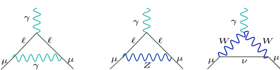
Figure 1: Feyman diagrams of the corrections to $a_{\mu}$on SM electroweak interactions.

Currently, the Standard Model (SM) of particle physics needs to be extended to explain signals or explore evidences of new physics like dark matter, neutrino masses, flavor universality violation, etc. There are different ways to extend the SM, and these ways open several alternatives to do physics beyond the SM. For example, to extend the SM gauge symmetry implies the existence of new gauge bosons. At least, by extending the symmetry just by a $U(1)_{x}$ group, we are predicting the existence of a new $Z$ boson. By extending the $SU(2)_{L}$ symmetry to a larger $SU(N)_{L}$ group, we have $N^{2}-4$ new gauge bosons at our disposal. Models based on the $SU(3)_{C}\times SU(4)_{L}\times U(1)_{X}$ 3-4-1 symmetry Pisano and Pleitez (1995), are that kind of beyond SM models. In this work we will focus in a very fundamental problem of particle physics, the anomalous magnetic moment of the muon, that we will describe in some detail below. The idea here is to study the different contributions to that anomaly arising in different versions of the 3-4-1 model. Our work is based on a rigorous correction to a numerical analysis previously carried out Cogollo (2015a, 2014, b), taking into account the most updated, model independent, analytical expressions that contributes to the anomaly Lindner et al. (2018), when compared to previous works Queiroz and Shepherd (2014) . It is important to mention that for elementary particles of mass m, electric charge q, and spin $\textbf{S}=\frac{1}{2}$, the Dirac equation predicts its magnetic dipole moment $\vec{\mu}$ , that it is an intrinsic property of the particle, given for the following relation:

$$\overrightarrow{\mu}=g\frac{q}{2m}\overrightarrow{s},$$ (1)

being $g$ the Landé g-factor or gyromagnetic ratio. For the muon, the prediction of the Dirac equation is $g_{\mu}=2$. Loop-level corrections generate little deviations from 2 – the anomalous magnetic moment, parametrized by $a_{\mu}=(g_{\mu}-2)/2$. $a_{\mu}$ allows us to test the SM since each sector yields a sizeable correction Tanabashi et al. (2018), that represents interactions of the type $\mu\rightarrow\gamma\mu$, which can be seen in the Feynman diagrams of the Fig.1. Nevertheless, there is a discrepancy between the Standard Model prediction and the experimental measurements, quantified by $\Delta a_{\mu}=a_{\mu}^{exp}-a_{\mu}^{SM}$, suggesting the presence of new physics that accounts for it. According to the Particle Data Group (PDG), the current discrepancy reads $a_{\mu}=a_{\mu}^{exp}-a_{\mu}^{SM}=(261\pm 78)\times 10^{-11}\,\,(3.3\sigma)$. The PDG review already acknowledges recent studies where the significance approaches $4\sigma$. However the large theoretical uncertainties can overshadow the significance of this discrepancy. It is important to mention that there are two experiments, the g-2 at FERMILAB Grange et al. (2015) and the Muon g-2 at J-PARC Abe et al. (2019), that will be able to decrease the error bar and increase the discrepancy if the central value remains the same. Having in mind the g-2 collaboration is about to announce new results, we find important to review previous studies in this matter in the context of the 3-4-1 gauge symmetry. Along with the actual discrepancy reported by PDG of $(3.3\sigma)$, we will use the projected discrepancy of the $g-2$ collaboration, $\Delta a_{\mu}=a_{\mu}^{exp}-a_{\mu}^{SM}=(261\pm 34)\times 10^{-11}\,\,(5\sigma)$, to impose the most stringent constraints on the scale of symmetry breaking and masses for three different versions of the 3-4-1 model, as aforementioned. The 3-4-1 symmetry is a natural extension of the $SU(3)_{C}\times SU(3)_{L}\times U(1)_{X}$ (3-3-1) symmetry that has been widely explored in the literature Pisano and Pleitez (1992); Foot et al. (1993). These 3-3-1 models can accommodate dark matter Fregolente and Tonasse (2003); Long and Lan (2003); de S. Pires and Rodrigues da Silva (2007); Mizukoshi et al. (2011a); Profumo and Queiroz (2014); Dong et al. (2013a, b); Queiroz (2015); Kelso et al. (2014a); Cogollo et al. (2014); Dong et al. (2014a, b); Mambrini et al. (2016); Alves et al. (2017); Carvajal et al. (2017); Dong et al. (2018); Montero et al. (2018); Arcadi et al. (2018); Huong et al. (2019), neutrino masses Montero et al. (2001); Tully and Joshi (2001); Montero et al. (2002); Cortez and Tonasse (2005); Cogollo et al. (2009); Queiroz et al. (2010); Cogollo et al. (2010, 2008); Okada et al. (2016); Vien et al. (2019); Cárcamo Hernández et al. (2018); Nguyen et al. (2018); de Sousa Pires et al. (2019); Cárcamo Hernández et al. (2019a, b, 2020), and also are entitled to a rich phenomenology concerning lepton flavor violation and collider physics Queiroz et al. (2010); Alves et al. (2011); Cogollo et al. (2012); Ruiz-Alvarez et al. (2012); Alves et al. (2013); Caetano et al. (2013); Dong et al. (2014a); Queiroz et al. (2016); Ferreira et al. (2019). 3-4-1 models embed these 3-3-1 models and therefore, we naturally inherit these features. As far as the muon anomalous magnetic moment is concerned several studies have been carried out in the past Kelso et al. (2014b, c); Binh et al. (2015a, b); De Conto and Pleitez (2017); Cogollo (2017); de Conto Santos (2018); de Jesus et al. (2020a), but 3-4-1 models experience different contributions to g-2, and that motive us to explore them in perspective with existing bounds.

In summary, we will investigate the corrections to $g_{\mu}-2$ in the context of 3-4-1 models. Our work is structured as follows: in Section II we present the models; in Section III we present our results; and later we conclude.

II $SU(4)_{L}\otimes U(1)_{X}$ Models

The 3-4-1 model is an electroweak extension of the SM, which is based on $SU(3)_{C}\otimes SU(4)_{L}\otimes U(1)_{X}$ gauge symmetry. In general, 3-4-1 models were proposed to provide an elegant solution to the neutrinos masses, by placing the leptons $\nu,e,\nu^{c}$ and $e^{c}$ in the same multiplet of a $SU(4)_{L}$ Pisano and Pleitez (1995). Today, we have different versions of the 3-4-1 model Dias et al. (2014); Palcu (2009a, b, c); Riazuddin and Fayyazuddin (2008) each of them inherits the features of their respective 3-3-1 model Pisano and Pleitez (1992). The most general expression for the electric charge operator in the case of the $SU(4)_{L}\otimes U(1)_{X}$ symmetry is given by:

$$Q=aT_{3L}+\frac{b}{\sqrt{3}}T_{8L}+\frac{c}{\sqrt{6}}T_{15L}+XI_{4},$$ (2)

where $a,b$ and $c$ are free parameters that allow us to set the fermion and scalar multiplets as well as the the gauge boson content. The $T_{iL}$ matrices are the generators of the $SU(4)_{L}$ group, defined as $T_{iL}=\lambda_{iL}/2$, being $\lambda_{iL}$ the Gell-Mann matrices for $SU(4)_{L}$. These gerenerators are normalized as Tr$(T_{i}T_{j})=\delta_{ij}/2$. Also, in the Eq.(2), $I_{4}$ is the $4\times 4$ identity matrix and $X$ is a quantum number, equivalent to the hypercharge in the SM. In the next section, we will briefly review the key theoretical aspects, which are relevant for the muon magnetic moment, for each one of the three different versions of the 3-4-1 model that we study here. Our goal is to reassess whether these models are capable of addressing the actual and projected discrepancy. In this way, we take interest in the interactions that can be represented as the Feynman diagram (Fig.1), but instead of SM leptons $\ell$ and gauge bosons Z and W, new fermions and new gauge bosons called $Z^{\prime}$, $W^{\prime}$ and U, will mediate these interactions, as will be explained below.

II.1 $SU(4)_{L}\otimes U(1)_{X}$ model with doubly charged gauge boson

In this model, the electric charge operator is defined as:

$$Q=\frac{1}{2}(\lambda_{3}-\frac{1}{\sqrt{3}}\lambda_{8}-\frac{2}{3}{\sqrt{6}}\lambda_{15})+X,$$ (3)

It is important to mention that in order to avoid anomalies, we must have the same number of $4$ and $4^{*}$ multiplets. For leptons, we have left and right-handed charged leptons and neutrinos in the same $SU(4)_{L}$ multiplet, that transform as $(1,4,0)$. The quark sector consists of one generation transforming as $(3,4,+2/3)$, and the two others as $(3,4^{*},-1/3)$ Pisano and Pleitez (1995). Concerning the right-handed quarks, they are all singlets under the symmetry in question. So, the fermionic content, excluding the right-handed quarks is:

$$\begin{array}[]{ccccc}f_{aL}=\left(\begin{array}[]{c}\nu_{a}\\ \ell_{a}\\ \nu_{a}^{c}\\ \ell_{a}^{c}\end{array}\right)_{L}\sim(1,4,0),\\ \\ Q_{1L}=\left(\begin{array}[]{c}u_{1}\\ d_{1}\\ u^{\prime}\\ J\end{array}\right)_{L}\sim(3,4,2/3),\\ \\ Q_{\alpha L}=\left(\begin{array}[]{c}j_{\alpha}\\ d_{\alpha}^{\prime}\\ u_{\alpha}\\ d_{\alpha}\end{array}\right)_{L}\sim(3,4^{*},-1/3).\end{array}$$ (21)

where $a=1,2,3$ is a flavor index, counting the number of fermion families, and $\alpha=2,3$.

An interesting characteristic of this model is the presence of new fermions beyond the SM ones, they are two new quarks $u^{\prime}$ and $J$ with charges $+2/3$ and $+5/3$ respectively, and another four $j_{2,3}$ and $d_{2,3}^{\prime}$ with charges $-4/3$ and $-1/3$, respectively.

In order to generate masses for all the quarks it is necessary to introduce three scalar multiplets $\eta$, $\rho$ and $\chi$, with just three of their neutral fields developing a vacuum expectation value, as we shown below:

$$\begin{array}[]{ccccc}\eta=\left(\begin{array}[]{c}\eta_{1}^{0}\\ \eta_{1}^{-}\\ \eta_{2}^{0}\\ \eta_{2}^{+}\end{array}\right)\sim(1,4,0),&\left<\eta\right>=(v_{1}/\sqrt{2},0,0,0),\\ \\ \rho=\left(\begin{array}[]{c}\rho_{1}^{+}\\ \rho^{0}\\ \rho_{2}^{+}\\ \rho^{++}\end{array}\right)\sim(1,4,+1),&\left<\rho\right>=(0,u/\sqrt{2},0,0),\\ \\ \chi=\left(\begin{array}[]{c}\chi_{1}^{-}\\ \chi^{--}\\ \chi_{2}^{-}\\ \chi^{0}\end{array}\right)\sim(1,4,-1),&\left<\chi\right>=(0,0,0,V_{\chi}/\sqrt{2}).\end{array}$$ (39)

As for the charged leptons and neutrinos masses it is necessary to introduce a Higgs multiplet transforming as $(1,10^{\ast},0)$ .

$$\begin{array}[]{ccccc}H=\left(\begin{array}[]{ccccc}H_{1}^{0}&H_{1}^{+}&H_{2}^{0}&H_{2}^{-}\\ H_{1}^{+}&H_{1}^{++}&H_{3}^{+}&H_{3}^{0}\\ H_{2}^{0}&H_{3}^{+}&H_{4}^{0}&H_{4}^{-}\\ H_{2}^{-}&H_{3}^{0}&H_{4}^{-}&H_{2}^{--}\end{array}\right)\sim(1,10^{*},0),\end{array}$$ (40)

with just three of their neutral fields developing a vaccum expectation value $\left<H_{2,3,4}^{0}\right>=v^{\prime\prime}$. It is important to mention that to preclude mixing among SM and the exotic quarks an extra multiplet $\eta^{\prime}$ must be introduced, transforming as $\eta$, but with different vacuum expectation value (VEV), $\langle\eta^{\prime}\rangle=(0,0,v^{\prime}/\sqrt{2},0)$. In this way we have that the symmetry breaking pattern occurs according to:

$$SU(4)_{L}\otimes U(1)_{X}\xrightarrow{\quad<\chi>\quad}SU(3)_{L}\otimes U(1)_{Z}$$

$$\xrightarrow{\quad<\eta^{\prime}>,<\eta>,<\rho>,<H>\quad}U(1)_{Q}.$$

As for the gauge sector it is important to remember that the gauge group we are working is the $SU(4)_{L}\times U(1)_{X}$, it implies that there are $15$ $W^{i}_{\mu}$ ($i=1,...,15$) gauge bosons belonging to the $SU(4)_{L}$ group, and there is a singlet boson $B_{\mu}$ owned by the $U(1)_{X}$ group. The electric charge and interactions of the gauge bosons beyond the SM ones is determined by the chose we did for the electric charge operator (3). In the diagonalization procedure we defined the physical charged gauge bosons as: $-\sqrt{2}W^{+}=W^{1}-iW^{2}$, $-\sqrt{2}V^{-}_{1}=W^{6}-iW^{7}$, $-\sqrt{2}V_{2}^{-}=W^{9}-iW^{10}$, $-\sqrt{2}V_{3}^{-}=W^{13}-iW^{14}$, $-\sqrt{2}U^{--}=W^{11}-iW^{12}$ and $\sqrt{2}X^{0}=W^{4}+iW^{5}$. Notice the presence of three new single charged vector bosons $V^{\pm}_{1,2,3}$ and the existence of a doubly charged vector boson $U^{--}$. As we will show, these new vector bosons generates contributions to the anomalous magnetic moment. In the approximation that we worked, $V^{\pm}_{1,2}$ are degenerates and its contribution to the anomaly is the same, say $\Delta a_{\mu V1,V2}$. The $V^{\pm}_{3}$ will be heavier than the other two $V^{\pm}_{1,2}$ bosons, $M^{2}_{V3}\approx 2\times M^{2}_{V1,V2}$, generating a $\Delta a_{\mu V3}\approx\frac{1}{2}\Delta a_{\mu V1,V2}$. The charged current interactions among the charged gauge bosons and the muon, relevant for the study of the anomaly, can be written as:

$${\cal L}^{CC}\supset-\frac{g}{2\sqrt{2}}[\overline{\nu}\gamma^{\mu}(1-\gamma_{5})\mu W^{+}_{\mu}+\overline{\nu^{c}}\gamma^{\mu}(1-\gamma_{5})\mu V^{+}_{1_{\mu}}+\overline{\mu^{c}}\gamma^{\mu}(1-\gamma_{5})\nu V^{+}_{2_{\mu}}+\overline{\mu^{c}}\gamma^{\mu}(1-\gamma_{5})\nu^{c}V^{+}_{3_{\mu}}+\overline{\mu^{c}}\gamma^{\mu}(1-\gamma_{5})\mu U^{++}_{\mu}]+H.C.,$$ (41)

being $g$ the coupling constant of the electroweak group. As for the neutral sector, there are four neutral gauge bosons, the massless photon and three massive ones $Z_{n}$, with $Z_{n}=Z_{N},Z,Z^{\prime}$ for $n=0,1,2$ respectively. To obtain the masses and the physical states in the neutral sector it is necessary to diagonalize the mass matrix in the basis $W^{3},W^{8},W^{15},B$, given by

$$\frac{g^{2}}{4}\left(\begin{array}[]{llll}v_{1}^{2}\!+\!u^{2}\!+2\!v^{\prime\prime 2}&\,\frac{1}{\sqrt{3}}(v_{1}^{2}\!-\!u^{2}\!-2\!v^{\prime\prime 2})&\,\frac{1}{\sqrt{6}}(v_{1}^{2}\!-\!u^{2}\!+\!4v^{\prime\prime 2})&\,-2tu^{2}\\ \frac{1}{\sqrt{3}}(v_{1}^{2}\!-\!u^{2}\!-2\!v^{\prime\prime 2})&\,\frac{1}{3}(v_{1}^{2}\!+\!4v^{\prime 2}\!+\!u^{2}\!+2\!v^{\prime\prime 2})&\frac{1}{3\sqrt{2}}(v_{1}^{2}\!-\!2v^{\prime 2}\!+\!u^{2}\!-4\!v^{\prime\prime 2})&\,\frac{2}{\sqrt{3}}tu^{2}\\ \frac{1}{\sqrt{6}}(v_{1}^{2}\!-\!u^{2}\!+\!4v^{\prime\prime 2})&\,\frac{1}{3\sqrt{2}}(v_{1}^{2}\!-\!2v^{\prime 2}\!+\!u^{2}\!-\!4v^{\prime\prime 2})&\,\frac{1}{6}(v_{1}^{2}+v^{\prime 2}+u^{2}+9V_{\chi}^{2}+8v^{\prime\prime 2})&\,\frac{2}{\sqrt{6}}t(u^{2}+3V_{\chi}^{2})\\ -2tu^{2}&\,\frac{2}{\sqrt{3}}tu^{2}&\,\frac{2}{\sqrt{6}}t(u^{2}\!+\!3V_{\chi}^{2})&4t^{2}(u^{2}\!+\!V_{\chi}^{2})\end{array}\right)$$ (42)

where $t=\frac{\sin\theta_{W}}{\sqrt{1-4\sin^{2}\theta_{W}}}$, being $\theta_{W}$ the electroweak angle. In principle, the diagonalization of (42) has to be done numerically. However, an analytic solution can be found by setting $v_{1}=u=v^{\prime\prime}$ and $v^{\prime}=V_{\chi}$, with $V_{\chi}\gg v_{1}$, yielding Pisano and Pleitez (1995)

$$M_{n}^{2}=\frac{g^{2}}{4}\lambda_{n}V_{\chi}^{2}$$ (43)

where $\lambda_{n}$ are constants given in the Appendix VI.1. As for the charged gauge bosons, its masses are given by,

$$M_{W}^{2}=\frac{g^{2}}{4}(4v_{1}^{2}),\quad M_{V_{1},2}^{2}=\frac{g^{2}}{4}(3v_{1}^{2}+V_{\chi}^{2}),$$ (44)

$$M_{V_{3}}^{2}=\frac{g^{2}}{4}(2v_{1}^{2}+2V_{\chi}^{2}),$$

$$M_{U^{++}}^{2}=\frac{g^{2}}{4}(9v_{1}^{2}+V_{\chi}^{2}).$$

To calculate the contributions to the anomaly coming from the neutral vector sector, we must have in hand the neutral currents, which are given by:

$${\cal L}^{NC}=-\frac{g}{2cos\theta_{W}}\left(\overline{\ell}_{L}\gamma^{\mu}\ell_{L}\alpha+\overline{\ell}_{R}\gamma^{\mu}\ell_{R}\beta\right)Z_{n\mu},$$ (45)

where $\alpha$ and $\beta$ are couplings that are given explicitly in the appendix VI.2.

The corrections coming from charged and neutral scalars would be derived from the Yukawa Lagrangian:

$$-{\cal L}_{Yuk}=\supset\frac{1}{2}G_{ab}\overline{f^{c}_{aL}}f_{bL}H,$$ (46)

where a,b= e, $\mu,\tau$. These scalars interact with leptons through the Yukawa Lagrangian in Eq (46), meaning that they couple to leptons proportionally to their masses. Hence, their contribution to $a_{\mu}$ will be suppressed. Finally, Fig.2 shows the Feynman diagrams of the interactions present in this model that contribute to the corrections $g_{\mu}-2$ .

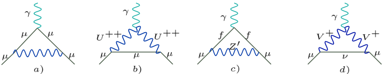
Figure 2: Feyman diagrams in order to contribute to the corrections to $a_{\mu}$in the $SU(4)_{L}\otimes U(1)_{X}$ model, coming from the interactions with new gauge bosons: a) and b) doubly-charged gauge boson ($U^{++}$), c) neutral gauge boson ($Z^{\prime}$) and d) singly charged bosons ($V^{+}$).

II.2 $SU(4)_{L}\otimes U(1)_{X}$ model without Exotic Electric Charges

In the $SU(4)_{L}\otimes U(1)_{X}$ model without Exotic Electric Charges Palcu (2012); Ponce et al. (2004), neutral heavy leptons are placed into the same multiplet that the left-handed charged leptons and neutrinos. All the right-handed fermions are singlets of $SU(4)_{L}$. In order to cancel all the quirial anomalies two left handed quark families must transform as 4-plets, and the other one as an anti-4-plet. So

$$\begin{array}[]{ccccc}f_{\alpha L}=\left(\begin{array}[]{c}\ell_{\alpha}\\ \nu_{\alpha}\\ N_{\alpha}\\ N_{\alpha}^{\prime}\end{array}\right)_{L}\sim(1,4^{*},-1/2),\\ \\ Q_{iL}=\left(\begin{array}[]{c}u_{i}\\ d_{i}\\ D_{i}\\ D_{i}^{\prime}\end{array}\right)_{L}\sim(3,4,-1/6),\\ \\ Q_{3L}=\left(\begin{array}[]{c}d_{3}\\ u_{3}\\ U\\ U^{\prime}\end{array}\right)_{L}\sim(3,4^{*},5/6),\end{array}$$ (64)

where $\alpha$ is the flavor index $\alpha=1,2,3$, and $i=1,2$.

As for the right handed fields, they transform as:

$$\left(e_{\alpha R}\right)\sim(\mathbf{1,1},-2),$$ (65)

$$\begin{array}[]{c}(d_{3R},(d_{iR}),(D_{iR}),(D_{iR}^{\prime})\sim(\mathbf{3},\mathbf{1},-2/3)\end{array}$$ (66)

$$(u_{3R}),(u_{iR}),(U_{R}),(U_{R}^{\prime})\sim(\mathbf{3},\mathbf{1},4/3)$$ (67)

The neutral heavy lepton masses are of the order $M_{N,N_{\alpha}^{\prime}}\approx V_{\chi}/2$.

In the scalar sector, this model contains four scalar multiplets that develop a vaccum expectection value as follows Palcu (2012)

$$\phi^{T}_{1} = (\zeta^{0},\zeta^{-}_{1},\zeta^{-}_{2},\zeta^{-}_{3})\sim[1,4,-3/2],\quad\left<\phi^{T}_{1}\right>=(v^{\prime},0,0,0)$$

$$\phi^{T}_{2} = (\rho^{+},\rho^{0}_{1},\rho^{0}_{2},\rho^{0}_{3})\sim[1,4,1/2],\quad\quad\left<\phi^{T}_{2}\right>=(0,v,0,0)$$

$$\phi^{T}_{3} = (\eta^{+},\eta^{0}_{1},\eta^{0}_{2},\eta^{0}_{3})\sim[1,4,1/2],\quad\quad\left<\phi^{T}_{3}\right>=(0,0,V,0)$$

$$\phi^{T}_{4} = (\chi^{+},\chi^{0}_{1},\chi^{0}_{2},\chi^{0}_{3})\sim[1,4,1/2].\quad\quad\left<\phi^{T}_{4}\right>=(0,0,0,V^{\prime})$$

This symmetry breaking pattern give masses to the fermions and gauge bosons of the model. The symmetry breaking occurs according to,

$$SU(4)_{L}\otimes U(1)_{X}\xrightarrow{<\phi^{T}_{4}>}SU(3)_{L}\otimes U(1)_{Z}$$

$$\xrightarrow{<\phi^{T}_{3}>}SU(2)_{L}\otimes U(1)_{Y}\xrightarrow{<\phi^{T}_{1}>,<\phi^{T}_{2}>}U(1)_{Q}.$$

the $SU(4)_{L}\otimes U(1)_{X}$ gauge group breaks down to $SU(3)_{L}\otimes U(1)_{Z}$ (3-3-1 model), by means of $<\phi^{T}_{4}>$ scalar boson. This latter group breaks down to $SU(2)_{L}\otimes U(1)_{Y}$ (gauge group of the SM) induced by $<\phi^{T}_{3}>$ scalar, and finally the last group breaks down to $U(1)_{Q}$, through two scalar bosons $<\phi^{T}_{1}>$ and $<\phi^{T}_{2}>$. In this work, we will work with the following simplifications for the VEVs $V\sim V^{\prime}>>v\sim v^{\prime}$. Since $M^{2}_{W^{\pm}}=\dfrac{g^{2}}{2}(v^{2}+v^{\prime 2})$ we have that $\sqrt{v^{2}+v^{\prime 2}}\approx 174Gev$ and then $v^{\prime}\sim 123Gev$

For simplicity we will explicitly show only the interactions that contribute to the anomaly in this version of the 3-4-1 model, for a detailed explanation of the gauge sector in this model check please Ponce et al. (2004)

$${\cal L}^{CC}_{l}\supset-\frac{g}{\sqrt{2}}\left[\overline{N}^{0}_{L}\gamma^{\mu}\mu_{L}K_{\mu}^{+}+\overline{N}_{L}^{0\prime}\gamma^{\mu}\mu_{L}X_{\mu}^{+}\right]+h.c.,$$

$${\cal L}^{NC}\supset\overline{\mu}\gamma^{\mu}[g_{V}-g_{A}\gamma^{5}]\mu Z^{\prime}_{\mu},$$ (68)

being:

$$g_{V}=-\frac{g}{2\cos\theta_{W}}\frac{1-3\sin^{2}\theta_{W}}{\sqrt{3\cos^{2}\theta_{W}-1}},$$

$$g_{A}=-\frac{g}{2\cos\theta_{W}}\frac{\cos^{2}\theta_{W}}{\sqrt{3\cos^{2}\theta_{W}-1}}$$ (69)

The mass eigenvalues of the gauge bosons we are interested here are:

$$M_{K^{\pm}}^{2}=\dfrac{g^{2}}{2}(V^{2}+v^{\prime 2}),M_{X^{\pm}}^{2}=\dfrac{g^{2}}{2}(V^{\prime 2}+v^{\prime 2}),$$ (70)

$$\quad M_{Z^{\prime}}^{2}=\dfrac{g^{2}}{4}V^{2}.$$

II.3 $SU(4)_{L}\otimes U(1)_{X}$ model with Exotic leptons

In the $SU(4)_{L}\otimes U(1)_{X}$ model with Exotic leptons Sánchez et al. (2008), instead of having neutral heavy leptons N, there are new exotic leptons denominated E. This lepton content is obtained by setting $a=b=c=1$ in the electric charge operator (2). The left-handed fermion multiplets of the model are

$$\begin{array}[]{ccccc}f_{\alpha L}=\left(\begin{array}[]{c}\nu_{\alpha}\\ \ell_{\alpha}\\ E_{\alpha}^{-}\\ E_{\alpha}^{\prime-}\end{array}\right)_{L}\sim(1,4,-3/4),\\ \\ Q_{iL}=\left(\begin{array}[]{c}d_{i}^{\prime}\\ u_{i}\\ U_{i}\\ U_{i}^{\prime}\end{array}\right)_{L}\sim(3,4^{*},5/12),\\ \\ Q_{3L}=\left(\begin{array}[]{c}u_{3}\\ d_{3}\\ D_{3}\\ D_{3}^{\prime}\end{array}\right)_{L}\sim(3,4,-1/12),\end{array}$$ (88)

and the right-handed particles are singlets of the $SU(4)_{L}$ symmetry.

$$e_{\alpha L}^{c}\sim(1,1,1),E_{\alpha L}^{c}\sim(1,1,1),E_{\alpha L}^{{}^{\prime}c}\sim(1,1,1)$$ (89)

$$\begin{array}[]{c}(d^{c}_{3L}),(d^{c}_{iL}),(D^{c}_{iL}),(D^{\prime c}_{iL})\sim(3^{*},1,+1/3),\\ (u^{c}_{3L}),(u^{c}_{iL}),(U^{c}_{L}),(U^{\prime c}_{L})\sim(3^{*},1,-2/3)\end{array}$$ (90)

where $i=1,2$ and $\alpha=1,2,3$. To generates masses for the fermions and the gauge bosons, it is necessary the following scalar content:

$$\phi^{T}_{1}=(\phi^{0}_{1},\phi^{+}_{1},\phi^{\prime+}_{1},\phi^{\prime\prime+}_{1})\sim[1,4^{*},3/4],\left<\phi^{T}_{1}\right>=(v_{3},0,0,0),$$

$$\phi^{T}_{2}=(\phi^{-}_{2},\phi^{0}_{2},\phi^{\prime 0}_{2},\phi^{\prime\prime 0}_{2})\sim[1,4^{*},-1/4],\left<\phi^{T}_{2}\right>=(0,v^{\prime},0,0),$$

$$\phi^{T}_{3}=(\phi^{-}_{3},\phi^{0}_{3},\phi^{\prime 0}_{3},\phi^{\prime\prime 0}_{3})\sim[1,4^{*},-1/4],\left<\phi^{T}_{3}\right>=(0,0,V,0),$$

$$\phi^{T}_{4}=(\phi^{-}_{4},\phi^{0}_{4},\phi^{\prime 0}_{4},\phi^{\prime\prime 0}_{4})\sim[1,4^{*},-1/4],\left<\phi^{T}_{4}\right>=(0,0,0,V_{\chi}),$$ (91)

The symmetry breaking occurs in the same way as in the previous model. We assume $V\approx V_{\chi}>>v_{3}\approx v^{\prime}$. The charged and neutral currents relevant for the anomaly are:

$${\cal L}^{CC}\supset-\frac{g}{2\sqrt{2}}\left(\overline{\mu}\gamma^{\mu}(1-\gamma^{5})EK^{0}_{\mu}+\overline{\mu}\gamma^{\mu}(1-\gamma^{5})E^{\prime}X^{0}_{\mu}\right),$$

$${\cal L}^{NC}\supset\overline{\ell}\gamma^{\mu}\left(g_{V}^{\prime}-g_{A}^{\prime}\gamma^{5}\right)\ell Z^{\prime},$$ (92)

where $K^{0}_{\mu}$, $X^{0}_{\mu}$ and $Z^{\prime}$ are the only ones beyond SM gauge bosons contributing to $g_{\mu}-2$ , and

$$g_{V}^{\prime}=\frac{g}{2\cos\theta_{W}}\frac{1/2+\sin^{2}\theta_{W}}{\sqrt{2-3\sin^{2}\theta_{W}}};$$

$$g_{A}^{\prime}=\frac{g}{2\cos\theta_{W}}\frac{\cos 2\theta_{W}}{2\sqrt{2-3\sin^{2}\theta_{W}}}$$ (93)

After the neutral fields acquire its vaccum expectation value, as decribed in (91), are generated the following mass terms for the bosons:

$$M^{2}_{W^{\pm}} = \frac{g^{2}}{2}(v_{3}^{2}+v^{\prime 2}),$$

$$M^{2}_{K^{0}}=\frac{g^{2}}{2}(v_{3}^{2}+V^{2}),$$ (94)

$$M^{2}_{X^{0}} = \frac{g^{2}}{2}(v_{3}^{2}+V_{\chi}^{2}),$$

being $g$ the coupling constant of the $SU(2)_{L}$ gauge group. As for the neutral gauge bosons, the $4\times 4$ mass matrix has a zero eigenvalue corresponding to the photon. For the remainder $3\times 3$ matrix we obtain the mass eigenvectors $Z_{\mu}$, $Z_{\mu}^{\prime}$ and $Z_{\mu}^{\prime\prime}$. In the approximation $V\sim V_{\chi}$, $Z_{\mu}^{\prime\prime}$ decouple from the other two, and it does not contributes to the anomaly, so it will be hereafter ignored. $Z_{\mu}$, $Z_{\mu}^{\prime}$ are still mixed,

$$\frac{g_{4}^{2}}{C^{2}_{W}}\left(\begin{array}[]{cc}v_{3}^{2}&\sqrt{2}\delta v^{2}_{3}S_{W}\\ \sqrt{2}\delta v_{3}^{2}S_{W}&\frac{2\delta^{2}}{S^{2}_{W}}[v_{3}^{2}(S^{4}_{W}+C^{4}_{W})+V^{2}C^{4}_{W}]\end{array}\right),$$ (95)

Here $g_{4}=g$, $\delta=g_{X}/(2g)$, and $g_{X}$ is the gauge coupling constants of the $U(1)_{X}$ group.

By diagonalizing this mass matrix we get the two physical neutral gauge bosons

$$Z_{1}^{\mu} = Z^{\mu}\cos\theta+Z^{\prime\mu}\sin\theta\;,$$

$$Z_{2}^{\mu} = -Z^{\mu}\sin\theta+Z^{\prime\mu}\cos\theta,$$ (96)

where the mixing angle is given by

$$\tan(2\theta)=\frac{2\sqrt{2}\delta v_{3}^{2}S^{3}_{W}}{2\delta^{2}[v_{3}^{2}(S^{4}_{W}+C^{4}_{W})+V^{2}C^{4}_{W}]-v_{3}^{2}S^{2}_{W}}.$$ (97)

III RESULTS

After presenting the key theoretical aspects of these three versions of the 3-4-1 model, now we will show our results. For each model, we calculated the individual contributions to the muon anomalous magnetic moment as function of the scale of symmetry breaking of the $SU(4)_{L}$ symmetry, $V_{\chi}$, and also, we computed the total contribution as function of $V_{\chi}$ to assess whether the model accommodates the anomaly or not. The analytical expressions used in this work are shown in the appendix VI.3, and were taken from Lindner et al. (2018). Besides, we provide the numerical codes we used to derive our results Villamizar and Cogollo (2020). As previously mentioned the corrections to $\Delta a_{\mu}$coming from scalar fields are suppressed by their couplings, which are proportional the muon mass, for this reason, we will ignore them in our calculations. In section III.4, we discuss how one can make the scalar corrections sizeable and meaningful to the g-2 anomaly. We will draw our conclusions having in mind lower mass bounds stemming from collider searches for new gauge bosons.

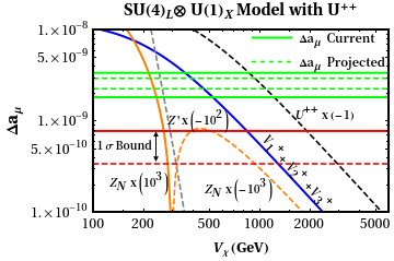
Figure 3: Individual contributions (left-panel) and total contribution (right-panel) to $\Delta a_{\mu}$as a function of the scale of symmetry breaking $V_{\chi}$, coming from the $SU(4)_{L}\otimes U(1)_{X}$ model with doubly charged gauge boson. The current and projected experimental bounds are exhibited with thick and dashed green lines respectively. The 1 $\sigma$ current and projected error are displayed as thick and dashed red lines respectively

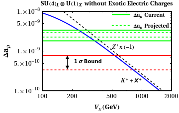
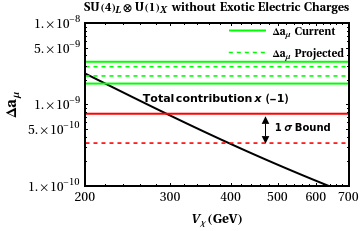
Figure 4: Individual contributions (left-panel) and total contribution (right-panel) to $\Delta a_{\mu}$as a function of the scale of symmetry breaking $V_{\chi}$, coming from the $SU(4)_{L}\otimes U(1)_{X}$ model without exotic electric charges for $M_{N}$=$M_{N^{\prime}}=10$GeV. The current and projected experimental bounds are exhibited with thick and dashed green lines respectively. The 1 $\sigma$ current and projected error are displayed as thick and dashed red lines respectively.

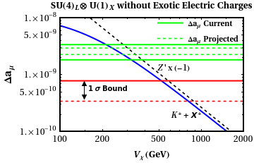
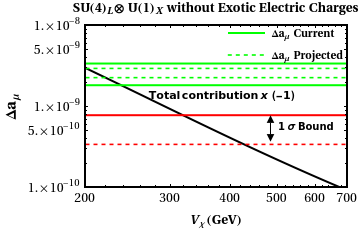
Figure 5: Individual contributions (left-panel) and total contribution (right-panel) to $\Delta a_{\mu}$as a function of the scale of symmetry breaking $V_{\chi}$, coming from the $SU(4)_{L}\otimes U(1)_{X}$ model without exotic electric charges for $M_{N}$=$M_{N^{\prime}}=100$GeV. The current and projected experimental bounds are exhibited with thick and dashed green lines respectively. The 1 $\sigma$ current and projected error are displayed as thick and dashed red lines respectively.

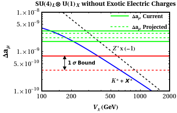
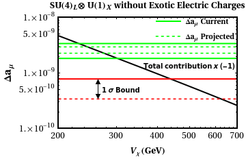
Figure 6: Individual contributions (left-panel) and total contribution (right-panel) to $\Delta a_{\mu}$as a function of the scale of symmetry breaking $V_{\chi}$, coming from the $SU(4)_{L}\otimes U(1)_{X}$ model without exotic electric charges for $M_{N}$=$M_{N^{\prime}}=1TeV$. The current and projected experimental bounds are exhibited with thick and dashed green lines respectively. The 1 $\sigma$ current and projected error are displayed as thick and dashed red lines respectively.

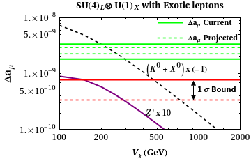
Figure 7: Individual contributions (left-panel) and total contribution (right-panel) to $\Delta a_{\mu}$as a function of the scale of symmetry breaking $V_{\chi}$, coming from the $SU(4)_{L}\otimes U(1)_{X}$ model with exotic leptons for $M_{E_{1}}$=$M_{E_{2}}=10$GeV. The current and projected experimental bounds are exhibited with thick and dashed green lines respectively. The 1 $\sigma$ current and projected error are displayed as thick and dashed red lines respectively.

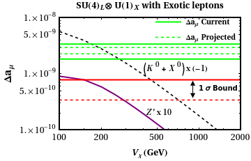
Figure 8: Individual contributions (left-panel) and total contribution (right-panel) to $\Delta a_{\mu}$as a function of the scale of symmetry breaking $V_{\chi}$, coming from the $SU(4)_{L}\otimes U(1)_{X}$ model with exotic leptons for $M_{E_{1}}$=$M_{E_{2}}=100$GeV. The current and projected experimental bounds are exhibited with thick and dashed green lines respectively. The 1 $\sigma$ current and projected error are displayed as thick and dashed red lines respectively.

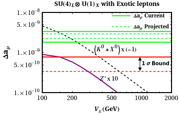
Figure 9: Individual contributions (left-panel) and total contribution (right-panel) to $\Delta a_{\mu}$as a function of the scale of symmetry breaking $V_{\chi}$, coming from the $SU(4)_{L}\otimes U(1)_{X}$ model with exotic leptons for $M_{E_{1}}$=$M_{E_{2}}=1TeV$. The current and projected experimental bounds are exhibited with thick and dashed green lines respectively. The 1 $\sigma$ current and projected error are displayed as thick and dashed red lines respectively.

Bounds	$V_{\chi}$(GeV)	$M_{V_{1}^{+},V_{2}^{+}}$(GeV)	$M_{V_{3}^{+}}$(GeV)	$M_{U^{++}}$(GeV)	$M_{Z^{\prime}}$(GeV)	$M_{Z_{N}}$(GeV)
$\sigma$ current	$\geq 1700$	$\geq 557$	$\geq 783$	$\geq 565$	$\geq 675$	$\geq 2048$
$\sigma$ projected	$\geq 2615$	$\geq 853$	$\geq 1203$	$\geq 858$	$\geq 1038$	$\geq 3150$

Table 1: Lower bounds on the scale of symmetry breaking $V_{\chi}$ and masses of the gauge bosons for the $SU(4)_{L}\otimes U(1)_{X}$ model with doubly charged gauge boson, for details see the text.

Models	Bounds	$M_{i}=10GeV$	$M_{i}=100GeV$	$M_{i}=1000GeV$
$SU(4)_{L}\otimes U(1)_{X}$ without exotic electric charges	$\sigma$ current	$V_{X}>293GeV$	$V_{X}>318GeV$	$V_{X}>438GeV$
		$M_{K^{+},X^{+}}>146GeV$	$M_{K^{+},X^{+}}>157GeV$	$M_{K^{+},X^{+}}>209GeV$
		$M_{Z^{\prime}}>95GeV$	$M_{Z^{\prime}}>103GeV$	$M_{Z^{\prime}}>142GeV$
	$\sigma$ projected	$V_{X}>394GeV$	$V_{X}>426GeV$	$V_{X}>624GeV$
		$M_{K^{+},X^{+}}>190GeV$	$M_{K^{+},X^{+}}>204GeV$	$M_{K^{+},X^{+}}>292GeV$
		$M_{Z^{\prime}}>128GeV$	$M_{Z^{\prime}}>138GeV$	$M_{Z^{\prime}}>203GeV$
$SU(4)_{L}\otimes U(1)_{X}$ with Exotic Leptons	$\sigma$ current	$V_{X}>466GeV$	$V_{X}>445GeV$	$V_{X}>365GeV$
		$M_{K^{0},X^{0}}>222GeV$	$M_{K^{0},X^{0}}>212GeV$	$M_{K^{0},X^{0}}>177GeV$
		$M_{Z^{\prime}}>340GeV$	$M_{Z^{\prime}}>327GeV$	$M_{Z^{\prime}}>273GeV$
	$\sigma$ projected	$V_{X}>719GeV$	$V_{X}>702GeV$	$V_{X}>578GeV$
		$M_{K^{0},X^{0}}>335GeV$	$M_{K^{0},X^{0}}>328GeV$	$M_{K^{0},X^{0}}>272GeV$
		$M_{Z^{\prime}}>515GeV$	$M_{Z^{\prime}}>503GeV$	$M_{Z^{\prime}}>418GeV$

Table 2: Lower bounds on the scale of symmetry breaking $V_{\chi}$ and masses of the gauge bosons for the $SU(4)_{L}\otimes U(1)_{X}$ model without exotic electric charges, for three different mass values of the neutral heavy leptons $N,N^{\prime}$, (Up panel). Lower bounds on the scale of symmetry breaking $V_{\chi}$ and masses of the gauge bosons for the $SU(4)_{L}\otimes U(1)_{X}$ model with exotic electric charges, for three different mass values of the exotic leptons $E_{1},E_{2}$, (down panel).

III.1 $SU(4)_{L}\otimes U(1)_{X}$ model with doubly charged gauge boson

First of all, let us remind the readers that in this version of the 3-4-1 model, we are working with the simplifications $v_{1}=u=v^{\prime\prime}$ and $v^{\prime}=V_{\chi}$, with $V_{\chi}\gg v_{1}$, and that $v_{1}\sim 123Gev$. In Fig.3 we show the individual contributions to $\Delta a_{\mu}$ as a function of the scale of symmetry breaking of the $SU(4)_{L}$ group, $V_{\chi}$. To assess whether this model accommodates the muon anomalous magnetic moment, we also show the total contribution of the model as function of $V_{\chi}$. We verify that the new neutral gauge bosons $Z^{\prime}$ and $Z_{N}$ have small and negative contributions to $\Delta a_{\mu}$. This occurs because in the limit $M_{Z^{\prime},Z_{N}}\gg m_{\mu}$, $m_{\mu}$ being the muon mass, their contributions to $\Delta a_{\mu}$are proportional to $g^{2}_{V}-5g^{2}_{A}$. The singly charged gauge bosons ($V^{+}_{1}+V^{+}_{2}+V^{+}_{3}$) corrections are positive, but not enough to compensate for the larger and negative contribution of the doubly charged gauge boson $U^{++}$. The sign of the contribution of the doubly charged gauge boson is due to the nature of its coupling with the muons. As was proved in Lindner et al. (2018), the $U^{++}$ couples to muons axially, its vector coupling is null. As the total contribution to the anomaly is negative, this model can not explain it, therefore, we can simply demand that the total contribution be smaller than the error bar. From the $1\sigma$ current bound, we obtain the lower limit $V_{\chi}>1700$ GeV; and $V_{\chi}>2615$ GeV from $1\sigma$ projected bound (see Fig.3). In accordance with the equation (43), these bounds translate into $M_{Z^{\prime}}\geq 675$ GeV and $M_{Z^{\prime}}\geq 1038$ GeV. These bounds are weaker than the LHC one for the $Z^{\prime}$ mass, which lies around $3.7$ TeV Nepomuceno and Meirose (2020) if the $Z^{\prime}$ boson decays exclusively into charged leptons. When exotic decays are present this limit weakens, but is yet stronger than the g-2 ones. It is important to emphasize that although this LHC limit has been derived for the minimal 3-3-1 model, it apply to our model also. This is because the 3-3-1 models are the low energy realization of 3-4-1 models. Each 3-3-1 version inherits the physical properties of some of the 3-4-1 models. Hence, the 3-4-1 we are working on it has the minimal 3-3-1 model as its low energy realization. As for the doubly charged gauge boson, our g-2 study translates into the following bounds, $M_{U^{++}}>565$ GeV and $M_{U^{++}}>858$ GeV using the $1\sigma$ current and projected bound, respectively. The most updated bound on the mass of this doubly charged gauge boson is $M_{U}\geq 1.2$ TeV Nepomuceno and Meirose (2020). For the singly charged bosons $V_{1}$ and $V_{2}$, using the $1\sigma$ current bound we obtain $M_{V1,V2}>556$ GeV and using the $1\sigma$ projected bound we obtain $M_{V1,V2}>852$ GeV. As for the singly charged boson $V_{3}$, using the $1\sigma$ current bound we obtain $M_{V3}>783$ GeV and using the $1\sigma$ projected bound we obtain $M_{V3}>1203$ GeV. The most updated bound on the mass of these singly charged gauge bosons reads $M_{V}\geq 850$ GeV Nepomuceno and Meirose (2020). Thus, despite not being able to address g-2, our study led to the strongest lower mass bound on the singly charged gauge boson.

III.2 $SU(4)_{L}\otimes U(1)_{X}$ without Exotic Electric Charges

In this model without Exotic Electric Charges we calculated the contributions to the anomaly by working with the following simplifications for the VEVs $V\sim V^{\prime}>>v\sim v^{\prime}$ and $v^{\prime}\sim 123$ GeV. In Figs.4, 5 and 6 we show the individual contributions to $\Delta a_{\mu}$ as a function of the scale of symmetry breaking, $V_{\chi}$, and as before, to assess whether this model accommodates the anomaly, we also show the total contribution of the model as function of $V_{\chi}$, for three different mass values of the neutral heavy leptons, $M_{N},M_{N^{\prime}}=10GeV$, $M_{N},M_{N^{\prime}}=100GeV$ and $M_{N},M_{N^{\prime}}=1TeV$ respectively. As we can see, for the three mass values of the neutral heavy leptons, the contribution of the neutral $Z^{\prime}$ is negative and greater than the positive $K^{+}+X^{+}$ contribution, producing a negative total contribution in all cases. Due to these negative contributions, we conclude that this model cannot explain $\Delta a_{\mu}$. As before, we just enforce that the total contribution be smaller than the error. By using the $1\sigma$ current and projected bounds, we derived the lower limits $V_{\chi}>293$ GeV, and $V_{\chi}>394$ GeV respectively, in the case $M_{N},M_{N^{\prime}}=10$ GeV. For the case $M_{N},M_{N^{\prime}}=100$ GeV, we derived the lower limit $V_{\chi}>318$ GeV by using the $1\sigma$ current bound, and $V_{\chi}>426$ GeV from $1\sigma$ projected bound. Finally, for the case $M_{N},M_{N^{\prime}}=1$ TeV, we get $V_{\chi}>438$ GeV by using the $1\sigma$ current bound, and $V_{\chi}>624$ GeV from $1\sigma$ projected bound. The lower limits on the masses of the $K^{+},X^{+}$ and $Z^{\prime}$ bosons for the different $M_{N},M_{N^{\prime}}$ values are shown in table II. As in the previous case, where the minimal 3-3-1 model inherits the physical properties of our 3-4-1 model with doubly charged gauge boson, in this case, the 3-3-1 model that inherits the properties of our 3-4-1 model without exotic electric charges, is the 3-3-1 LHN Mizukoshi et al. (2011b); Cataño M. et al. (2012). The collider bounds derived for this 3-3-1 version are similar to the bounds derived for the 3-3-1 RHN model Long (1996a, b). For the 3-3-1 RHN model the collider bound has been derived as $M_{Z^{\prime}}\geq 4$ TeV Lindner et al. (2018), that would translate into a lower bound $V_{\chi}\geq 12$ TeV. In the 3-3-1 LHN model this bound can be weakened if we consider additional decay modes, as exotic quarks and the neutral heavy leptons itself. Including these decay modes, the bound is read now as $M_{Z^{\prime}}\geq 2$ TeV or $V_{\chi}\geq 6$ TeV de Jesus et al. (2020a), still strongest than the bounds derived from the g-2.

III.3 $SU(4)_{L}\otimes U(1)_{X}$ with Exotic leptons

For the 3-4-1 model with exotic leptons the symmetry breaking pattern is such that $V\approx V_{\chi}>>v_{3}\approx v^{\prime}=123$ GeV. In Figs.7, 8 and 9 we show the total and individual contributions to $\Delta a_{\mu}$ as a function of the scale of symmetry breaking, $V_{\chi}$, for three different mass values of the exotic heavy leptons, $M_{E_{1}},M_{E_{2}}=10GeV$, $M_{E_{1}},M_{E_{2}}=100$ GeV and $M_{E_{1}},M_{E_{2}}=1$ TeV respectively. As we can see, for all mass values of the exotic leptons, the contribution of the bosons $K^{0}+X^{0}$ is negative and greater than the low and positive contribution of the $Z^{\prime}$ boson. Therefore, the total contributions are always negative, and for this reason this version of the 3-4-1 model can not explain $\Delta a_{\mu}$. What we have left is to derive some constraints demanding that the total contribution be less than the error, as we did for the other models. By using the $1\sigma$ current bound, we derived the lower limit $V_{\chi}>466$ GeV, and $V_{\chi}>719$ GeV from $1\sigma$ projected bound, for the case $M_{E_{1}},M_{E_{2}}=10$ GeV. For the case $M_{E_{1}},M_{E_{2}}=100$ GeV, we derived the lower limit $V_{\chi}>445$ GeV by using the $1\sigma$ current bound, and $V_{\chi}>702$ GeV from $1\sigma$ projected bound. Finally, for the case $M_{E_{1}},M_{E_{2}}=1$ TeV, we derived the lower limit $V_{\chi}>365$ GeV by using the $1\sigma$ current bound, and $V_{\chi}>578$ GeV from $1\sigma$ projected bound. The lower limits on the masses of the $K^{0}$, $X^{0}$ and $Z^{\prime}$ bosons for the different $M_{N},M_{N^{\prime}}$ values are shown in table II. One can clearly see that even for the case where $V_{\chi}>719$ GeV (the greater value of $V_{\chi}$), the lower mass limit $M_{Z^{\prime}}\geq 515$ GeV is weak and far from the existing collider bound.

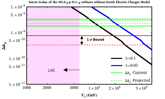
Figure 10: Inert scalar contribution to $\Delta a_{\mu}$as a function of the scale of symmetry breaking $V_{\chi}$, for the $SU(4)_{L}\otimes U(1)_{X}$ model without exotic electric charges. The current and projected experimental bounds are exhibited with thick and dashed green lines respectively. The 1 $\sigma$ current and projected error are displayed as thick and dashed red lines respectively. For when $\Lambda=0.1$ the model accommodate the anomaly for $8Tev\leq V_{\chi}\leq 11Tev$, and for when $\Lambda=0.05$ the model accommodate the anomaly for $16Tev\leq V_{\chi}\leq 22Tev$.

III.4 Alternative paths

We have demonstrated that all three models based on 3-4-1 symmetry we investigated in this work cannot accommodate the muon anomalous magnetic moment. Therefore, a natural question arises. Can we make these models simultaneously consistent with the g-2 anomaly and the existing collider bounds? The answer is yes. We remind the reader that the scalar contributions to g-2 are dwindled because they couple to muons proportional to the muon mass (see for example Eq 11 from de Jesus et al. (2020a)). As was pointed out in de Jesus et al. (2020a) and most recently in de Jesus et al. (2020b), a way to salvage these extended gauge sectors is by introducing inert scalars, or heavy vector-like charged leptons plus singlet scalars (in the case the vector-like heavy lepton be a singlet of the gauge symmetry). Here we will address how the first of these ideas can be implemented in the 3-4-1 model without exotic electric charges. As was shown in the section II.2, in this model we dispose of four scalars multiplets transforming as $\sim 4$ by the $SU(4)_{L}$ symmetry. All of them develop vacuum expectation value, and for this reason they are not inert scalars and their interactions with fermions are proportional to the fermion mass. We now introduce a new inert scalar $\phi_{1}^{\prime}$, which is a replica of $\phi_{1}$ . The Yukawa lagrangian that generates contributions to the muon anomaly is now:

$${\cal L}^{Y}=f_{\alpha,\beta}\overline{f}_{\alpha L}\phi_{1}^{\star}\ell_{\beta R}+\lambda_{\alpha,\beta}\overline{f}_{\alpha L}\phi_{1}^{\prime\star}\ell_{\beta R}+H.C.$$ (98)

For the case of the $\phi_{1}$ scalar, the interactions are:

$$f_{\alpha,\beta}\left(\overline{\ell}_{\alpha L}\zeta^{0\star}\ell_{\beta R}+\overline{\nu}_{\alpha L}\zeta_{1}^{+}\ell_{\beta R}+\overline{N}_{\alpha L}\zeta_{2}^{+}\ell_{\beta R}+\overline{N^{\prime}}_{\alpha L}\zeta_{3}^{+}\ell_{\beta R}\right).$$

As the $\phi_{1}$ multiplet develops vacuum expectation value, its interactions with fermions are proportional to the fermion mass. For simplicity let us check the diagonal interaction $f_{2,2}\overline{\mu}_{L}R_{\zeta}\mu_{R}$. In this case $f_{2,2}\sim\frac{m_{\mu}}{v^{\prime}}\sim 10^{-4}$, and $R_{\zeta}$ is the mass eigenvector obtained after the diagonalization procedure in the neutral scalar sector. The other three diagonal interactions among the muon, singly charged scalars, and neutral leptons, share the same $f_{2,2}$ coupling. As $f_{2,2}\sim 10^{-4}$ and $\Delta a_{\mu}$ is proportional to the square of this coupling constant, all the conributions coming from $\phi_{1}$ are irrelevants . As for the interactions $\lambda_{\alpha,\beta}\left(\overline{\ell}_{\alpha L}\zeta^{\prime 0\star}\ell_{\beta R}+\overline{\nu}_{\alpha L}\zeta_{1}^{\prime+}\ell_{\beta R}+\overline{N}_{\alpha L}\zeta_{2}^{\prime+}\ell_{\beta R}+\overline{N^{\prime}}_{\alpha L}\zeta_{3}^{\prime+}\ell_{\beta R}\right)$ coming from the $\phi_{1}^{\prime}$ inert scalar, the situation is very different. As $\phi_{1}^{\prime}$ is inert, the diagonal coupling $\lambda_{2,2}$ (as well as any other $\lambda_{\alpha,\beta}$) is not proportional to the fermion mass. Again let us check the first of the interactions, $\lambda_{2,2}\overline{\mu}_{L}\zeta^{\prime 0\star}\mu_{R}$, this coupling (and the others proportional to $\lambda_{2,2}$, among the muon, charged scalars and neutral leptons, like $\sim\lambda_{2,2}\overline{N}_{2L}\zeta_{2}^{\prime+}\mu_{R}$) contributes to the anomaly. The mass of the $\phi^{\prime}_{1}$ scalar comes from the potential terms $\sim\Lambda\phi_{3}^{\dagger}\phi_{3}\phi_{1}^{\prime\dagger}\phi_{1}^{\prime}+\Lambda\phi_{4}^{\dagger}\phi_{4}\phi_{1}^{\prime\dagger}\phi_{1}^{\prime}$. After $\phi_{3},\phi_{4}$ develop vacuum expectation value, the scalar $\phi_{1}^{\prime}$ gains mass proportional to $M_{\phi_{1}^{\prime}}\sim\Lambda V_{\chi}$. By setting the parameter $\lambda_{2,2}=1$ and using the equation (121) of appendix VI.3.4, we calculated the main contribution of $\phi_{1}^{\prime}$ to the anomaly for two different values of $\Lambda$ (see figure 10) . For when $\Lambda=0.1$ the model accommodate the anomaly for $8Tev\leq V_{\chi}\leq 11$  TeV, and for when $\Lambda=0.05$ the model accommodate the anomaly for $16{\rm TeV}\leq V_{\chi}\leq 22$ TeV.

IV conclusions

We have revisited the muon anomalous magnetic moment in the context of the $SU(3)_{C}\times SU(4)_{L}\times U(1)_{X}$ symmetry. We have used updated and correct analytical expressions to obtain the corrections to g-2. Our numerical results differ from previous works, but the overall conclusions are basically the same, that is, the models can not accommodate the g-2 anomaly and the bounds on the scale of symmetry breaking rising from g-2 are weaker than the ones coming from collider searches. A key point overlooked in the past is the contribution from the doubly charged gauge boson ,$U^{++}$, which is negative and not positive as previously assumed. Moreover, we also derived new bounds on the scale of symmetry breaking of these models in the light of the upcoming results of the g-2 experiment at FERMILAB. We concluded that none of these models can accommodate the discrepancy among the theory and the current and projected experimental results. As a final contribution of this work, we presented a way via inert scalars to salvage these models. Basically, we look for inert scalars multiplets that couple to leptons multiplets in an invariant way. These inert multiplets are replicas of the scalar multiplets that couple with leptons and generates its masses. That allowed us to address g-2 while being consistent with current collider bounds.

V ACKNOWLEDGEMENTS

DC is partly supported by the Brazilian National Council for Scientific and Technological Development (CNPq), under grants 436692/2018-0. YSV acknowledges the financial support from CAPES under grants 88882.375870/2019-01. YMOT acknowledges the financial support from CAPES under grants 88887.485509/2020-00.

VI Appendix

VI.1 Masses of the gauge bosons: $SU(4)_{L}\otimes U(1)_{X}$ model with doubly charged gauge boson

Coupling constants that appear in the neutral boson mass equation Eq.43.

$$\lambda_{n}=\frac{1}{3}\left[A+2\left(A^{2}+3B\right)^{\frac{1}{2}}\cos\left(\frac{2n\pi+\Theta}{3}\right)\right],$$ (99)

where,

$$A=3+4t^{2}+(7+4t^{2})a^{2},B=-2\left[1+3t^{2}+2(4+9t^{2})a^{2}\right],$$ (100)

$$C=8(1+4t^{2})a^{2},\quad\Theta=\arccos\left[\frac{2A^{3}+9AB+27C}{2(A^{2}+3B)^{\frac{3}{2}}}\right],$$ (101)

with $a\equiv v_{1}/V_{\chi}$, and $t=g^{\prime}/g$.

VI.2 Vector and axial couplings: $SU(4)_{L}\otimes U(1)_{X}$ model with doubly charged gauge boson

The derivation of the vector and axial couplings is a bit tedious, our results agree with Ref.Pisano and Pleitez (1995). Defining,

$$Z_{n\mu}\approx x_{n}W^{3}_{\mu}+y_{n}W^{8}_{\mu}+z_{n}W^{15}_{\mu}+w_{n}B_{\mu},$$ (102)

with

$$x_{n}=-\frac{2a^{2}}{t}\frac{1-3t^{2}+(1-t^{2})a^{2}-(1-2t^{2})\lambda_{n}}{D_{n}(t,a)}w_{n},$$ (103)

$$y_{n} = \frac{1}{\sqrt{3}t}\frac{2(2+t^{2})a^{2}-10a^{4}t^{2}-\left[1+(1-4t^{2})a^{2}\right]\lambda_{n}}{D_{n}(t,a)}w_{n},$$ (104)

$$z_{n}=\frac{1}{\sqrt{6}t}\frac{8(2+t^{2})a^{2}+4(3+2t^{2})a^{4}-4\left[1+2(2+t^{2})a^{2}\right]\lambda_{n}+3\lambda_{n}^{2}}{D_{n}(t,a)}w_{n},$$ (105)

$$w^{2}_{n}=\frac{1}{1+x_{n}^{2}/w_{n}^{2}+y_{n}^{2}/w_{n}^{2}+z_{n}^{2}/w_{n}^{2}},$$ (106)

and finally

$$D_{n}(t,a)=2(7+5a^{2})-(3+13a^{2})\lambda_{n}+2\lambda_{n}^{2}.$$ (107)

The vector and axial couplings can be derived from the Lagrangian

$${\cal L}=-\frac{g}{2C_{W}}\left(\overline{l_{L}}\gamma^{\mu}l_{L}\alpha+\overline{l_{R}}\gamma^{\mu}l_{R}\beta\right)Z_{n\mu},$$ (108)

with

$$\alpha=-c_{W}\left(-x_{n}+\frac{1}{\sqrt{3}}y_{n}+\frac{1}{\sqrt{6}}z_{n}+\frac{4}{3}w_{n}t\right)+\frac{4}{3}c_{W}w_{n}t,\quad\beta=-\frac{3}{\sqrt{6}}z_{n}.$$ (109)

with $Z_{0}=Z_{N},Z_{1}=Z,Z_{2}=Z^{\prime}$.

VI.3 Analytical Expressions for the Muon Magnetic Moment

The analytical expressions for all the contributions to $g_{\mu}-2$ that have been used in the present manuscript were taken from Lindner et al. (2018).

VI.3.1 Charged Fermion – Doubly Charged Vector Boson

The contribution to the muon anomalous magnetic moment coming from a doubly charged vector boson is derived from the following general lagrangian

$$\mathcal{L}_{\textrm{int}}=g^{ij}_{V}U^{++}_{\mu}\,\overline{\ell_{i}^{C}}\gamma^{\mu}\,\ell_{j}+g^{ij}_{A}U^{++}_{\mu}\,\overline{\ell_{i}^{C}}\gamma^{\mu}\gamma^{5}\ell_{j}+\mathrm{h.c.}$$ (110)

In this case, $g_{\mu}-2$ is given by:

$$\Delta a_{\mu}\left(U^{++}\right) =\frac{8}{8\pi^{2}}\frac{m_{\mu}^{2}}{m_{U}^{2}}\int_{0}^{1}{d}x\frac{g_{V}^{2}P_{1}^{+}(x)+g_{A}^{2}P_{1}^{-}(x)}{\epsilon_{f}^{2}\lambda^{2}(1-x)\left(1-\epsilon_{f}^{-2}x\right)+x}$$

$$+\frac{4}{8\pi^{2}}\frac{m_{\mu}^{2}}{m_{U}^{2}}\int_{0}^{1}{d}x\frac{g_{V}^{2}P_{2}^{+}(x)+g_{A}^{2}P_{2}^{-}(x)}{(1-x)\left(1-\lambda^{2}x\right)+\epsilon_{f}^{2}\lambda^{2}x},$$ (111)

with $\epsilon_{f}\equiv\frac{m_{f}}{m_{\mu}}$ and $\lambda\equiv\frac{m_{\mu}}{m_{U}}$. This contribution arises in the first model, the model with doubly charged gauge boson, where ${m}_{f}={m}_{\mu}$. The polynomials inside the integrals are defined as:

$$P_{1}^{\pm}=-2x^{2}(1+x\mp 2\epsilon_{f})+\lambda^{2}x(1-x)(1\mp\epsilon_{f})^{2}(x\pm\epsilon_{f}),$$ (112)

and

$${P}_{2}^{\pm}=2x\left(1-x\right)\left(x-2\pm 2{\epsilon}_{f}\right)+{\lambda}^{2}{x}^{2}{\left(1\mp{\epsilon}_{f}\right)}^{2}\left(1-x\pm{\epsilon}_{f}\right)$$ (113)

As was pointed out in the text, the $U^{++}$ couples to muons axially, its vector coupling is null. Taking this into account, and the fact that $\epsilon_{f}=1$, the polynomials that enter in the contribution are reduced to:

$${P}_{1}^{-}\left(x\right)=-2{x}^{2}(x+3)+4{\lambda}^{2}x(1-x){(x-1)},$$ (114)

$${P}_{2}^{-}\left(x\right)=2{x}(1-x)(x-4)-4{\lambda}^{2}{x}^{3}$$ (115)

From the integral (111) and using the polynomials (114) and (115) above, we have obtained the contribution of the $U^{++}$ boson. We remember the readers that these expressions (111), (114) and (115) have been derived in a revisited work Lindner et al. (2018), that differs from the expressions derived in a previous work Queiroz and Shepherd (2014) used in the reference Cogollo (2015a). The differences between the two results are the signal of the second integral in (111) and the signal of the first term of the polynomial (114). This is the reason why the contribution of the $U^{++}$ boson has changed of sign when compared with the previous work Cogollo (2015a).

VI.3.2 Neutral Fermion - Charged Gauge Boson

In the case where a neutral lepton couples to a charged gauge boson and a muon through the following general lagrangian

$$\mathcal{L}_{\mathrm{int}}=g_{V}^{ij}W^{\prime+}_{\mu}\overline{N_{i}}\gamma^{\mu}\ell_{j}+g_{A}^{ij}W^{\prime+}_{\mu}\overline{N_{i}}\gamma^{\mu}\gamma^{5}\ell_{j}+\textrm{h.c.}$$ (116)

a contribution to $g_{\mu}-2$ is generated

$$\Delta a_{\mu}(N,W^{\prime})=-\frac{m_{\mu}^{2}}{8\pi^{2}M_{W^{\prime}}^{2}}\int_{0}^{1}dx\frac{g^{2}_{V}{P}_{1}^{+}(x)+g^{2}_{A}{P}_{1}^{-}(x)}{{\epsilon}_{f}^{2}\lambda^{2}(1-x)(1-{\epsilon}_{f}^{-2}x)+x},$$ (117)

where $\lambda=m_{\mu}/M_{W^{\prime}}$, ${\epsilon}_{f}=m_{{N}_{f}}/m_{\mu}$ and $P_{1}^{\pm}$ is defined in the Eq. (112). For the first model, model with doubly charged gauge boson, $m_{{N}_{f}}={m}_{\nu}$ and the mediators are the $V$ bosons. As for the second model, model without exotic electric charges, $m_{{N}_{f}}={m}_{N}={m}_{N^{{}^{\prime}}}$, and the mediators are the $K^{+},X^{+}$ bosons.

VI.3.3 Charged lepton - Neutral Gauge Boson.

In the case where a charged lepton couples to a neutral gauge boson and a muon through the following general lagrangian

$$\mathcal{L}_{\mathrm{int}}=g_{V}^{ij}Z^{\prime}_{\mu}\overline{E_{i}}\gamma^{\mu}\ell_{j}+g_{A}^{ij}Z^{\prime}_{\mu}\overline{E_{i}}\gamma^{\mu}\gamma^{5}\ell_{j}+\textrm{h.c.}$$ (118)

a contribution to $g_{\mu}-2$ is generated

$$\Delta a_{\mu}(Z^{\prime})=\frac{m_{\mu}^{2}}{8\pi^{2}M_{Z^{\prime}}^{2}}\int_{0}^{1}dx\frac{g^{2}_{V}{P}_{2}^{+}(x)+g^{2}_{A}{P}_{2}^{-}(x)}{(1-x)(1-\lambda^{2}x)+{\epsilon}_{f}^{2}\lambda^{2}x},$$ (119)

where $\lambda=m_{\mu}/M_{Z^{\prime}}$, ${\epsilon}_{f}=m_{E_{f}}/m_{\mu}$, and $P_{2}^{\pm}$ is defined in the Eq. (113). For the first model, model with doubly charged gauge boson, ${m}_{E_{f}}={m}_{\mu}$ and the mediators are the ${Z}^{{}^{\prime}}$ and the ${Z}_{N}$ bosons. For the second model, model without exotic electric charge, ${m}_{E_{f}}={m}_{\mu}$ and the mediator is the ${Z}^{{}^{\prime}}$ boson. As for the third model, model with exotic electric charges, ${m}_{E_{f}}={m}_{E}={m}_{E^{\prime}}$ for when the mediators are the bosons $K^{0},X^{0}$, and ${m}_{E_{f}}={m}_{\mu}$ for when the mediator is the ${Z}^{{}^{\prime}}$ boson.

VI.3.4 Neutral Scalar

If there are additional electrically neutral scalar fields in a model, interacting with muons through the following Lagrangian

$$\mathcal{L}_{\textrm{int}}=g_{s}^{ij}\phi\,\overline{\ell_{i}}\,\ell_{j}+ig_{p}^{ij}\phi\,\overline{\ell_{i}}\gamma^{5}\ell_{j},$$ (120)

they will induce a correction to $g_{\mu}-2$ given by:

$$\Delta a_{\mu}(\phi)=\frac{m_{\mu}^{2}}{8\pi^{2}M_{\phi}^{2}}\int_{0}^{1}dx\frac{g^{2}_{s}{P}_{3}^{+}(x)+g^{2}_{p}{P}_{3}^{-}(x)}{(1-x)(1-\lambda^{2}x)+{\epsilon}_{f}^{2}\lambda^{2}x},$$ (121)

where

$${P}_{3}^{\pm}={x}^{2}\left(1-x\pm{\epsilon}_{f}\right),$$ (122)

and with $\epsilon_{f}={m}_{f}/{m}_{\mu}$ and $\lambda=m_{\mu}/m_{\phi}$. From (121) we have derived the contributions to the anomaly of the neutral scalars $\zeta^{0\star}$ and $\zeta^{\prime 0\star}$. In both cases ${m}_{f}={m}_{\mu}$. As for the coupling constants we have $g_{p}=0$ for $\zeta^{0\star}$ and $\zeta^{\prime 0\star}$, $g_{s}\sim\frac{m_{\mu}}{v^{\prime}}$ for the $\zeta^{0\star}$ scalar and $g_{s}=\lambda_{2,2}\sim 1$ for the $\zeta^{\prime 0\star}$ scalar. It is important to emphasize that the contributions to $\Delta a_{\mu}$ are proportional to the square of the coupling constant, then the contribution generated by $\zeta^{\prime 0\star}$ is $\sim 10^{8}$ times greater than the contribution coming from $\zeta^{0\star}$.

VI.3.5 Singly Charged Scalar

The relevant interaction terms for the contribution to $g_{\mu}-2$ of a scalar with unit charge, are given by

$$\mathcal{L}_{\textrm{int}}=g_{s}^{ij}\phi^{+}\,\overline{\nu_{i}}\,\ell_{j}+g_{p}^{ij}\phi^{+}\,\overline{\nu_{i}}\gamma^{5}\ell_{j}+\ \mathrm{h.c.}$$ (123)

In this case, $g_{\mu}-2$ is given by:

$$\Delta a_{\mu}\left(\phi^{+}\right)=-\frac{1}{8\pi^{2}}\frac{m_{\mu}^{2}}{m_{\phi^{+}}^{2}}\int_{0}^{1}\mathrm{d}x\,\sum_{f}\frac{g_{s}^{2}P_{4}^{+}(x)+g_{p}^{2}P_{4}^{-}(x)}{\epsilon_{f}^{2}\lambda^{2}(1-x)\left(1-\epsilon_{f}^{-2}x\right)+x},$$ (124)

where

$$P_{4}^{\pm}(x)=x(1-x)\left(x\pm\epsilon_{f}\right),\quad\epsilon_{f}\equiv\frac{m_{f}}{m_{\mu}},\quad\lambda\equiv\frac{m_{\mu}}{m_{\phi^{+}}}.$$ (125)

For the singly charged scalars of the $\phi_{1}$ multiplet ($\zeta_{1}^{+},\zeta_{2}^{+},\zeta_{3}^{+}$), $g_{s}=g_{p}\sim\frac{m_{\mu}}{v^{\prime}}$, and their contributions to the anomaly, besides being negatives, are irrelevants. As for the singly charged scalars of the $\phi_{1}^{\prime}$ multiplet ($\zeta_{1}^{\prime+},\zeta_{2}^{\prime+},\zeta_{3}^{\prime+}$), $g_{s}=g_{p}=\lambda_{2,2}\sim 1$, and their contributions are $\sim 10^{8}$ times greater than the contributions coming from $\phi_{1}$. Besides the contributions of the singly charged scalars belonging to the inert scalar $\phi_{1}^{\prime}$ be large and negatives, (see Fig.11), it is the contribution of the $\zeta^{\prime 0\star}$ the dominant one, by far. Even when we add up the individual contributions of all the particles of the model, this total contribution basically coincides with the individual contribution of the $\zeta^{\prime 0\star}$ particle, as we can see in Fig.12.

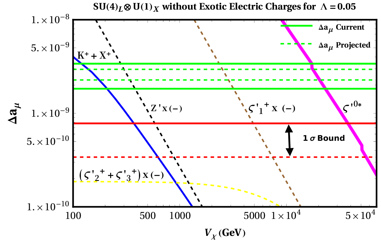
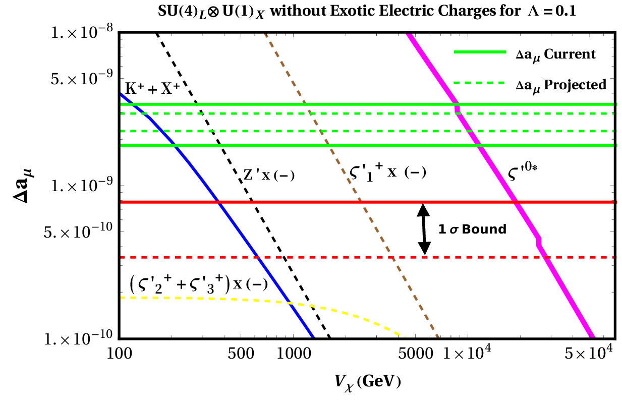
Figure 11: Individual contributions to $\Delta a_{\mu}$ including the inert scalar, as a function of the scale of symmetry breaking $V_{\chi}$, coming from the model without exotic electric charges, for $M_{N}$=$M_{N^{\prime}}=1TeV$. $\Lambda=0.05$ (up-panel) $\Lambda=0.1$ (down-panel).The current and projected experimental bounds are exhibited with thick and dashed green lines respectively. The 1 $\sigma$ current and projected error are displayed as thick and dashed red lines respectively.

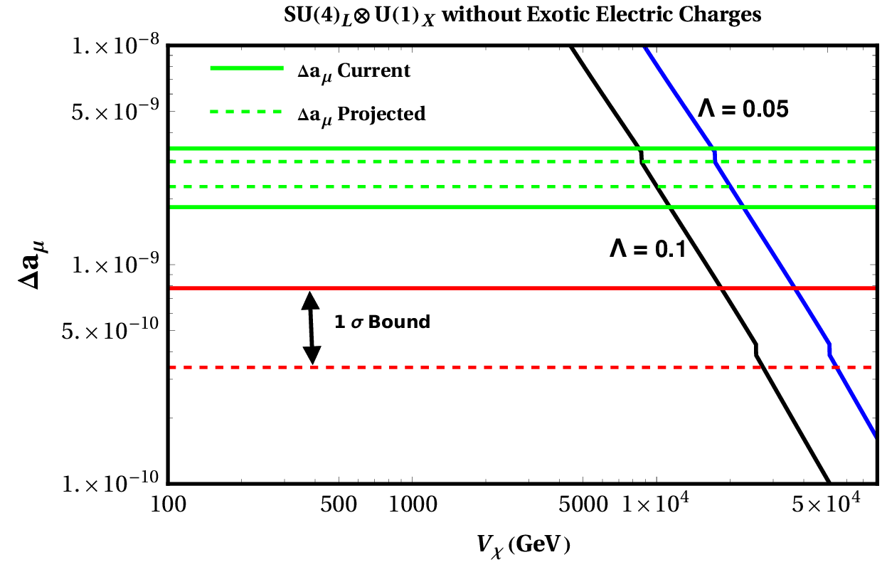
Figure 12: Total contribution to $\Delta a_{\mu}$ including the inert scalar, as a function of the scale of symmetry breaking $V_{\chi}$, coming from the model without exotic electric charges, for $M_{N}$=$M_{N^{\prime}}=1TeV$. $\Lambda=0.05$ (Blue line) $\Lambda=0.1$ (black line).The current and projected experimental bounds are exhibited with thick and dashed green lines respectively. The 1 $\sigma$ current and projected error are displayed as thick and dashed red lines respectively.

In the integral (124) we have used $m_{f}=m_{\nu}$ for the $\zeta_{1}^{+}$ and $\zeta_{1}^{\prime+}$ particles, and $m_{f}=m_{N}=m_{N^{\prime}}$ for $\zeta_{2}^{+},\zeta_{2}^{\prime+},\zeta_{3}^{+},\zeta_{3}^{\prime+}$.

References

- Pisano and Pleitez (1995) F. Pisano and V. Pleitez, Phys. Rev. D51, 3865 (1995), arXiv:hep-ph/9401272 [hep-ph] .
- Cogollo (2015a) D. Cogollo, Int. J. Mod. Phys. A30, 1550038 (2015a), arXiv:1409.8115 [hep-ph] .
- Cogollo (2014) D. Cogollo, (2014), 10.3844/pisp.2015.42.50, arXiv:1411.2810 [hep-ph] .
- Cogollo (2015b) D. Cogollo, Int. J. Mod. Phys. A30, 1550187 (2015b), arXiv:1508.01492 [hep-ph] .
- Lindner et al. (2018) M. Lindner, M. Platscher, and F. S. Queiroz, Phys. Rept. 731, 1 (2018), arXiv:1610.06587 [hep-ph] .
- Queiroz and Shepherd (2014) F. S. Queiroz and W. Shepherd, Phys. Rev. D 89, 095024 (2014), arXiv:1403.2309 [hep-ph] .
- Tanabashi et al. (2018) M. Tanabashi et al. (Particle Data Group), Phys. Rev. D98, 030001 (2018).
- Grange et al. (2015) J. Grange et al. (Muon g-2), (2015), arXiv:1501.06858 [physics.ins-det] .
- Abe et al. (2019) M. Abe et al., PTEP 2019, 053C02 (2019), arXiv:1901.03047 [physics.ins-det] .
- Pisano and Pleitez (1992) F. Pisano and V. Pleitez, Phys. Rev. D46, 410 (1992), arXiv:hep-ph/9206242 [hep-ph] .
- Foot et al. (1993) R. Foot, O. F. Hernandez, F. Pisano, and V. Pleitez, Phys. Rev. D47, 4158 (1993), arXiv:hep-ph/9207264 [hep-ph] .
- Fregolente and Tonasse (2003) D. Fregolente and M. D. Tonasse, Phys. Lett. B555, 7 (2003), arXiv:hep-ph/0209119 [hep-ph] .
- Long and Lan (2003) H. N. Long and N. Q. Lan, Europhys. Lett. 64, 571 (2003), arXiv:hep-ph/0309038 [hep-ph] .
- de S. Pires and Rodrigues da Silva (2007) C. A. de S. Pires and P. S. Rodrigues da Silva, JCAP 0712, 012 (2007), arXiv:0710.2104 [hep-ph] .
- Mizukoshi et al. (2011a) J. K. Mizukoshi, C. A. de S. Pires, F. S. Queiroz, and P. S. Rodrigues da Silva, Phys. Rev. D83, 065024 (2011a), arXiv:1010.4097 [hep-ph] .
- Profumo and Queiroz (2014) S. Profumo and F. S. Queiroz, Eur. Phys. J. C74, 2960 (2014), arXiv:1307.7802 [hep-ph] .
- Dong et al. (2013a) P. V. Dong, T. P. Nguyen, and D. V. Soa, Phys. Rev. D88, 095014 (2013a), arXiv:1308.4097 [hep-ph] .
- Dong et al. (2013b) P. V. Dong, H. T. Hung, and T. D. Tham, Phys. Rev. D87, 115003 (2013b), arXiv:1305.0369 [hep-ph] .
- Queiroz (2015) F. S. Queiroz, AIP Conf. Proc. 1604, 83 (2015), arXiv:1310.3026 [astro-ph.CO] .
- Kelso et al. (2014a) C. Kelso, C. A. de S. Pires, S. Profumo, F. S. Queiroz, and P. S. Rodrigues da Silva, Eur. Phys. J. C 74, 2797 (2014a), arXiv:1308.6630 [hep-ph] .
- Cogollo et al. (2014) D. Cogollo, A. X. Gonzalez-Morales, F. S. Queiroz, and P. R. Teles, JCAP 1411, 002 (2014), arXiv:1402.3271 [hep-ph] .
- Dong et al. (2014a) P. V. Dong, D. T. Huong, F. S. Queiroz, and N. T. Thuy, Phys. Rev. D90, 075021 (2014a), arXiv:1405.2591 [hep-ph] .
- Dong et al. (2014b) P. V. Dong, N. T. K. Ngan, and D. V. Soa, Phys. Rev. D90, 075019 (2014b), arXiv:1407.3839 [hep-ph] .
- Mambrini et al. (2016) Y. Mambrini, S. Profumo, and F. S. Queiroz, Phys. Lett. B 760, 807 (2016), arXiv:1508.06635 [hep-ph] .
- Alves et al. (2017) A. Alves, G. Arcadi, P. Dong, L. Duarte, F. S. Queiroz, and J. W. F. Valle, Phys. Lett. B 772, 825 (2017), arXiv:1612.04383 [hep-ph] .
- Carvajal et al. (2017) C. D. R. Carvajal, B. L. Sánchez-Vega, and O. Zapata, Phys. Rev. D96, 115035 (2017), arXiv:1704.08340 [hep-ph] .
- Dong et al. (2018) P. Dong, D. Huong, F. S. Queiroz, J. W. F. Valle, and C. Vaquera-Araujo, JHEP 04, 143 (2018), arXiv:1710.06951 [hep-ph] .
- Montero et al. (2018) J. C. Montero, A. Romero, and B. L. Sánchez-Vega, Phys. Rev. D97, 063015 (2018), arXiv:1709.04535 [hep-ph] .
- Arcadi et al. (2018) G. Arcadi, C. Ferreira, F. Goertz, M. Guzzo, F. S. Queiroz, and A. Santos, Phys. Rev. D 97, 075022 (2018), arXiv:1712.02373 [hep-ph] .
- Huong et al. (2019) D. T. Huong, D. N. Dinh, L. D. Thien, and P. Van Dong, JHEP 08, 051 (2019), arXiv:1906.05240 [hep-ph] .
- Montero et al. (2001) J. C. Montero, C. A. de S. Pires, and V. Pleitez, Phys. Lett. B502, 167 (2001), arXiv:hep-ph/0011296 [hep-ph] .
- Tully and Joshi (2001) M. B. Tully and G. C. Joshi, Phys. Rev. D64, 011301 (2001), arXiv:hep-ph/0011172 [hep-ph] .
- Montero et al. (2002) J. C. Montero, C. A. De S. Pires, and V. Pleitez, Phys. Rev. D65, 095001 (2002), arXiv:hep-ph/0112246 [hep-ph] .
- Cortez and Tonasse (2005) N. V. Cortez and M. D. Tonasse, Phys. Rev. D72, 073005 (2005), arXiv:hep-ph/0510143 [hep-ph] .
- Cogollo et al. (2009) D. Cogollo, H. Diniz, and C. A. de S. Pires, Phys. Lett. B677, 338 (2009), arXiv:0903.0370 [hep-ph] .
- Queiroz et al. (2010) F. Queiroz, C. de S.Pires, and P. da Silva, Phys. Rev. D 82, 065018 (2010), arXiv:1003.1270 [hep-ph] .
- Cogollo et al. (2010) D. Cogollo, H. Diniz, and C. A. de S. Pires, Phys. Lett. B687, 400 (2010), arXiv:1002.1944 [hep-ph] .
- Cogollo et al. (2008) D. Cogollo, H. Diniz, C. A. de S. Pires, and P. S. Rodrigues da Silva, Eur. Phys. J. C58, 455 (2008), arXiv:0806.3087 [hep-ph] .
- Okada et al. (2016) H. Okada, N. Okada, and Y. Orikasa, Phys. Rev. D93, 073006 (2016), arXiv:1504.01204 [hep-ph] .
- Vien et al. (2019) V. V. Vien, H. N. Long, and A. E. Cárcamo Hernández, Mod. Phys. Lett. A34, 1950005 (2019), arXiv:1812.07263 [hep-ph] .
- Cárcamo Hernández et al. (2018) A. E. Cárcamo Hernández, H. N. Long, and V. V. Vien, Eur. Phys. J. C78, 804 (2018), arXiv:1803.01636 [hep-ph] .
- Nguyen et al. (2018) T. P. Nguyen, T. T. Le, T. T. Hong, and L. T. Hue, Phys. Rev. D97, 073003 (2018), arXiv:1802.00429 [hep-ph] .
- de Sousa Pires et al. (2019) C. A. de Sousa Pires, F. Ferreira De Freitas, J. Shu, L. Huang, and P. Wagner Vasconcelos Olegário, Phys. Lett. B797, 134827 (2019), arXiv:1812.10570 [hep-ph] .
- Cárcamo Hernández et al. (2019a) A. E. Cárcamo Hernández, N. A. Pérez-Julve, and Y. Hidalgo Velásquez, Phys. Rev. D100, 095025 (2019a), arXiv:1907.13083 [hep-ph] .
- Cárcamo Hernández et al. (2019b) A. E. Cárcamo Hernández, Y. Hidalgo Velásquez, and N. A. Pérez-Julve, Eur. Phys. J. C79, 828 (2019b), arXiv:1905.02323 [hep-ph] .
- Cárcamo Hernández et al. (2020) A. E. Cárcamo Hernández, L. T. Hue, S. Kovalenko, and H. N. Long, (2020), arXiv:2001.01748 [hep-ph] .
- Alves et al. (2011) A. Alves, E. Ramirez Barreto, A. Dias, C. de S.Pires, F. Queiroz, and P. Rodrigues da Silva, Phys. Rev. D 84, 115004 (2011), arXiv:1109.0238 [hep-ph] .
- Cogollo et al. (2012) D. Cogollo, A. de Andrade, F. Queiroz, and P. Rebello Teles, Eur. Phys. J. C 72, 2029 (2012), arXiv:1201.1268 [hep-ph] .
- Ruiz-Alvarez et al. (2012) J. Ruiz-Alvarez, C. de S.Pires, F. S. Queiroz, D. Restrepo, and P. Rodrigues da Silva, Phys. Rev. D 86, 075011 (2012), arXiv:1206.5779 [hep-ph] .
- Alves et al. (2013) A. Alves, E. Ramirez Barreto, A. Dias, C. de S.Pires, F. S. Queiroz, and P. Rodrigues da Silva, Eur. Phys. J. C 73, 2288 (2013), arXiv:1207.3699 [hep-ph] .
- Caetano et al. (2013) W. Caetano, C. A. de S. Pires, P. S. Rodrigues da Silva, D. Cogollo, and F. S. Queiroz, Eur. Phys. J. C 73, 2607 (2013), arXiv:1305.7246 [hep-ph] .
- Queiroz et al. (2016) F. S. Queiroz, C. Siqueira, and J. W. F. Valle, Phys. Lett. B 763, 269 (2016), arXiv:1608.07295 [hep-ph] .
- Ferreira et al. (2019) M. M. Ferreira, T. B. de Melo, S. Kovalenko, P. R. Pinheiro, and F. S. Queiroz, Eur. Phys. J. C 79, 955 (2019), arXiv:1903.07634 [hep-ph] .
- Kelso et al. (2014b) C. Kelso, P. Pinheiro, F. S. Queiroz, and W. Shepherd, Eur. Phys. J. C 74, 2808 (2014b), arXiv:1312.0051 [hep-ph] .
- Kelso et al. (2014c) C. Kelso, H. Long, R. Martinez, and F. S. Queiroz, Phys. Rev. D 90, 113011 (2014c), arXiv:1408.6203 [hep-ph] .
- Binh et al. (2015a) D. Binh, D. Huong, and H. Long, Zh. Eksp. Teor. Fiz. 148, 1115 (2015a), arXiv:1504.03510 [hep-ph] .
- Binh et al. (2015b) D. T. Binh, D. T. Huong, L. T. Hue, and H. N. Long, Commun. Phys. 25, 29 (2015b).
- De Conto and Pleitez (2017) G. De Conto and V. Pleitez, JHEP 05, 104 (2017), arXiv:1603.09691 [hep-ph] .
- Cogollo (2017) D. Cogollo, (2017), arXiv:1706.00397 [hep-ph] .
- de Conto Santos (2018) G. de Conto Santos, Electron and muon anomalous magnetic dipole moment in the 3-3-1 model with heavy leptons, Ph.D. thesis, Sao Paulo, IFT (2018).
- de Jesus et al. (2020a) A. S. de Jesus, S. Kovalenko, F. S. Queiroz, C. A. S. Pires, and Y. S. S. Villamizar, (2020a), arXiv:2003.06440 [hep-ph] .
- Dias et al. (2014) A. G. Dias, P. R. D. Pinheiro, C. A. de S. Pires, and P. S. Rodrigues da Silva, Annals Phys. 349, 232 (2014), arXiv:1309.6644 [hep-ph] .
- Palcu (2009a) A. Palcu, Mod. Phys. Lett. A24, 1247 (2009a), arXiv:0902.1301 [hep-ph] .
- Palcu (2009b) A. Palcu, Mod. Phys. Lett. A24, 1731 (2009b), arXiv:0902.1828 [hep-ph] .
- Palcu (2009c) A. Palcu, Int. J. Mod. Phys. A24, 4923 (2009c), arXiv:0902.3756 [hep-ph] .
- Riazuddin and Fayyazuddin (2008) Riazuddin and Fayyazuddin, Eur. Phys. J. C56, 389 (2008), arXiv:0803.4267 [hep-ph] .
- Long et al. (2016) H. N. Long, L. T. Hue, and D. V. Loi, Phys. Rev. D 94, 015007 (2016).
- Palcu (2012) A. Palcu, Phys. Rev. D 85, 113010 (2012), arXiv:1111.6262 [hep-ph] .
- Ponce et al. (2004) W. A. Ponce, D. A. Gutiérrez, and L. A. Sánchez, Physical Review D 69 (2004), 10.1103/physrevd.69.055007.
- Sánchez et al. (2008) L. A. Sánchez, L. A. Wills-Toro, and J. I. Zuluaga, Phys. Rev. D 77, 035008 (2008).
- Villamizar and Cogollo (2020) O. T. Y. M. Villamizar, Yoxara S and D. Cogollo, Mathematica numerical codes of the Muon Anomalous Magnetic Moment to 341 Models (Accessed in 2020), https://1drv.ms/u/s!AmXaqAgFnBmhhMtAedFJ4G9PW2ub7w?e=othbcq.
- Nepomuceno and Meirose (2020) A. Nepomuceno and B. Meirose, Phys. Rev. D101, 035017 (2020), arXiv:1911.12783 [hep-ph] .
- Mizukoshi et al. (2011b) J. K. Mizukoshi, C. A. de S. Pires, F. S. Queiroz, and P. S. Rodrigues da Silva, Phys. Rev. D 83, 065024 (2011b).
- Cataño M. et al. (2012) E. Cataño M., R. Martínez, and F. Ochoa, Phys. Rev. D 86, 073015 (2012).
- Long (1996a) H. N. Long, Phys. Rev. D 54, 4691 (1996a).
- Long (1996b) H. N. Long, Phys. Rev. D 53, 437 (1996b).
- de Jesus et al. (2020b) A. S. de Jesus, S. Kovalenko, F. S. Queiroz, K. Sinha, and C. Siqueira, “Vector-like leptons and inert scalar triplet: Lepton flavor violation, and collider searches,” (2020b), arXiv:2004.01200 [hep-ph] .