Generalized Bloch band theory for non-Hermitian bulk-boundary correspondence

Abstract

Bulk-boundary correspondence is the cornerstone of topological physics. In some non-Hermitian topological systems this fundamental relation is broken in the sense that the topological number calculated for the Bloch energy band under the periodic boundary condition fails to reproduce the boundary properties under the open boundary. To restore the bulk-boundary correspondence in such non-Hermitian systems a framework beyond the Bloch band theory is needed. We develop a non-Hermitian Bloch band theory based on a modified periodic boundary condition that allows a proper description of the bulk of a non-Hermitian topological insulator in a manner consistent with its boundary properties. Taking a non-Hermitian version of the Su-Schrieffer-Heeger model as an example, we demonstrate our scenario, in which the concept of bulk-boundary correspondence is naturally generalized to non-Hermitian topological systems.

I Introduction

In topological insulators Kane and Mele (2005a, b); Bernevig et al. (2006); König et al. (2007); Hasan and Kane (2010); Hatsugai (1993); Ryu and Hatsugai (2002) non-trivial topology of the bulk wave function is unambiguously related to the appearance of mid-gap boundary states. This relation often referred to as bulk-boundary correspondenceHatsugai (1993); Ryu and Hatsugai (2002) highlights the physics of topological insulator. However, it has been pointed out that this concept cannot be trivially applied to some non-Hermitian topological insulators.Yao and Wang (2018) In these systems Bloch band theory fails to encode nontrivial boundary properties in the bulk energy band,Yokomizo and Murakami (2019) thus breaking superficially the bulk-boundary correspondence. To restore the bulk-boundary correspondence a framework beyond the standard Bloch band theory is needed.

Making quantum mechanics non-Hermitian might have been regarded as an act of heresy. Hatano and Nelson (1996, 1997) The parity-time symmetric non-Hermitian systems with real eigenvalues Bender and Boettcher (1998) might have been less guilty; indeed such systems have been much studied. Makris et al. (2008); Hodaei et al. (2014); Feng et al. (2014); Regensburger et al. (2012); Guo et al. (2009); Rüter et al. (2010); Mochizuki et al. (2016); Xiao et al. (2017) But after a decade or so, non-Hermitian quantum mechanics is now regarded as real. Poli et al. (2015); Zhao et al. (2018); Diehl et al. (2011); Feng et al. (2017); Zhen et al. (2015); Zhou et al. (2018) The non-Hermitian generalization of a topological insulator has also started to be considered in this context Esaki et al. (2011); Hu and Hughes (2011). Since then, an increasing number of papers have appeared in this field, Lee (2016); Yao and Wang (2018); Yokomizo and Murakami (2019); Longhi (2019); Borgnia et al. (2020); Martinez Alvarez et al. (2018); Kunst et al. (2018); Xiong (2018); Herviou et al. (2019); Kunst and Dwivedi (2019); Zirnstein et al. (2019); Lee and Thomale (2019); Torres (2019); Zhang et al. (2019); Okuma et al. (2020); Li et al. (2020); Lee and Longhi (2020) including a remarkable proposal of a practical application, the topological insulator laser. Parto et al. (2018); Weimann et al. (2016); Bandres et al. (2018); Harari et al. (2018)

A nontrivial feature of a topological insulator is in its energy spectrum under an open boundary condition (obc). Let us consider, for simplicity, a one-dimensional model of topological insulator of length $L$. If $L$ is sufficiently large, the energy eigenvalues arrange themselves into quasi continuous energy bands, which we will simply call bulk energy bands.Yokomizo and Murakami (2019) Such bulk energy bands also allows us to introduce an energy gap and the concept of an insulator. For the system to be topologically non-trivial, there must appear boundary states in the enegy gap, and such boundary states must be protected by a bulk topological number. In an infinite Hermitian crystal such a topological number is expressed as an integral with respect to $k$ over the entire Brillouin zone ($k\in[0,2\pi]$),Thouless et al. (1982); Kohmoto (1985) where $k$ specifies a Bloch function:

$$\psi(x)=e^{ikx}u(x).$$ (1)

$u(x)$ is its periodic part satisfying $u(x+1)=u(x)$, and the lattice constant $a$ is chosen to be unity ($a=1$).

Figure 1(a) [top annex panel] shows typical energy spectra of a non-Hermitian topological system [Su-Schrieffer-Heeger (SSH) model with non-reciprocal hopping]. The blue spectrum represents the one in the boundary geometry; i.e., under the obc, where contributions from the bulk and from the boundary combine to give the full spectrum. Between the two gap closing points $P_{1}$ and $P_{2}$ there appears a pair of mid-gap boundary states. The gray spectrum represents the one in the bulk geometry under the periodic boundary condition (pbc). Note that in the Hermitian limit the bulk geometry is equivalent to the Bloch band theory under the pbc. Here, in a non-Hermitian example, the number and positions of the gap closing points $Q_{1-4}$ in the bulk geometry (gray/pbc spectrum) are different from the ones in the boundary geometry (blue/obc spectrum), clearly indicating that the bulk energy band in the Bloch band theory based on the pbc fails to achieve the bulk-boundary correspondence.

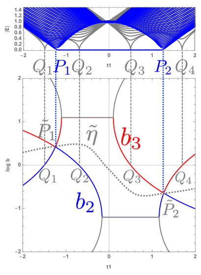
(a) (b)

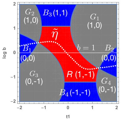
Figure 1: Schematic illustration of the non-Hermitian bulk-boundary correspondence. The two main panels show how to decode the topological information encoded in the spectra of a non-Hermitian SSH model [extra panel on top of panel (a), the blue (gray) curves represent the spectrum under the open (periodic) boundary condition]. The model is explicitly given in Eqs. (15), (16) and (17). Parameters: $t_{2}=1$, $t_{3}=0.1$, $\gamma_{1}=0.5$, $\gamma_{2}=0.1$.

In the above example of a non-Hermitian topological insulator,Yao and Wang (2018); Yokomizo and Murakami (2019) the bulk energy bands under the obc are very different from the ones in the Bloch band theory under the pbc. Under the obc the corresponding eigen wave function is not a superposition of the plane-wave Bloch form (1), but rather of the following generalized Bloch form:

$$\psi(x)=\beta^{x}u(x).$$ (2)

Unless $|\beta|=1$, such a wave function damps (or amplifies) exponentially, and tends to be localized in the vicinity of an end of the system. This phenomenon is often referred to as non-Hermitian skin effect, and typical to systems with non-reciprocal hopping.Lee (2016); Yao and Wang (2018); Yokomizo and Murakami (2019); Longhi (2019); Martinez Alvarez et al. (2018); Kunst et al. (2018); Xiong (2018); Herviou et al. (2019); Kunst and Dwivedi (2019); Zirnstein et al. (2019); Lee and Thomale (2019) Note that Eq. (2) is clearly incompatible with the pbc: $\psi(x+L)=\psi(x)$ unless $|\beta|=1$.

We have previously established Imura and Takane (2019) that by considering a modified periodic boundary condition (mpbc): $\psi(x+L)=b^{L}\psi(x)$ with $b$ being a real positive constant, less restrictive than the standard pbc, one can restore the desired correspondence between the boundary and the bulk properties. In this paper, we perform a detailed description of the bulk of this system in this scenario, which was lacking in Ref. Imura and Takane, 2019, leading to a non-Hermitian generalization of the Bloch band theory compatible with the bulk-boundary correspondence scenario.

The argument of Ref. Imura and Takane, 2019 on the bulk-boundary correspondence was based on a smooth deformation to the Hermitian limit. Here, we give a more general argument supporting that the bulk-boundary correspondence proposed in Ref. Imura and Takane, 2019 is valid also in the non-perturbative non-Hermitian regime. To demonstrate our scenario we consider a one-dimensional ($d=1$) model; e.g., Hatano-Nelson model and a non-Hermitian generalization of the SSH model. Yet, the underlying idea can be equally applied to systems with higher spatial dimensions ($d=2,3$). Our approach can be also applied to other class of models, e.g., for a system with symplectic symmetry. Kawabata et al. (2020); Okuma et al. (2020) The authors of Refs. Yao and Wang, 2018; Yokomizo and Murakami, 2019 proposed an alternative scenario that extracts the information on the boundary properties from the bulk energy band under the obc (i.e., the continuum part of the obc spectrum). This scenario takes only the boundary geometry into consideration. We, on the contrary, employ the genuine bulk geometry under the mpbc to extract the information on the boundary properties. Unlike the non-Bloch approach of Refs. Yao and Wang, 2018; Yokomizo and Murakami, 2019, our scenario may be regarded as a natural generalization of the Bloch band theory to non-Hermitian system. Note that our generalized Bloch band theory includes the conventional Hermitian Bloch band theory as a special case of $b=1$.

II Hermitian and Non-Hermitian Bloch band theories

II.1 Generalized Bloch function under the mpbc

Let us consider the eigenstates of an electron in a crystal. Let the Hamiltonian $H$ possess a lattice translational symmetry; $H$ commutes with the lattice translation operator $\Xi$ such that $[\Xi,H]=0$, where $\Xi$ acts on the eigenstate (eigen bra) $\langle x|$ of the coordinate $x$ such that $\langle x|\Xi=\langle x+1|$. Here, we have chosen the lattice constant $a$ to be unity ($a=1$). Let $|\beta\rangle$ be a simultaneous eigenstate of $H$ and $\Xi$,

$$H|\beta\rangle = E(\beta)|\beta\rangle,$$

$$\Xi|\beta\rangle = \beta|\beta\rangle.$$ (3)

The wave function defined by $\psi(x)=\langle x|\beta\rangle$ satisfies the relation:

$$\psi(x+1)=\langle x|\Xi|\beta\rangle=\beta\langle x|\beta\rangle=\beta\psi(x),$$ (4)

implying that $\psi(x)$ takes the generalized Bloch form (2). In an infinite crystal the wave function $\psi(x)$ must be bounded wherever in the system governed by Hermitian quantum mechanics. This imposes $|\beta|=1$, or $\beta=e^{ik}$ with $k\in[0,2\pi]$, and hence $\psi(x)$ reduces to the standard Bloch form (1). When $\beta$ takes continuous values on a unit circle in the complex $\beta$-pane, the trajectory of $E(\beta)$ defines a Bloch energy band. Thus, the range of $k\in[0,2\pi]$, or equivalently, the unit circle in the $\beta$-plane defines the Brillouin zone (BZ) for a Hermitian crystal.

Applying a pbc is standard in the conventional Bloch band theory and allows one to reconstitute the above continuous energy band, starting with a system of finite length $L$ and taking the limit $L\rightarrow\infty$ at the end of the calculation. The pbc: $\psi(x+L)=\psi(x)$ imposes $\beta^{L}=1$, i.e., $\beta=e^{ik}$ with $k=2\pi n/L$, $n=0,1,2,\cdots,L-1$. Namely, the pbc, without making reference to the boundedness of the wave function, automatically selects from the generalized Bloch form (2), those wave functions that have the standard plane-wave like form (1) with $|\beta|=1$.

The pbc is technically important for an unambiguous formulation of the Bloch band theory, avoiding difficulties arising from the continuous values of $k$ in an infinite system. In Hermitian topological band insulators the pbc plays the role of bulk geometry, in which purely bulk states appear in the spectrum. The existence and identification of such a geometry is indispensable for achieving the bulk-boundary correspondence. However, in non-Hermitian systems the pbc fails to play a proper role of such a bulk geometry.

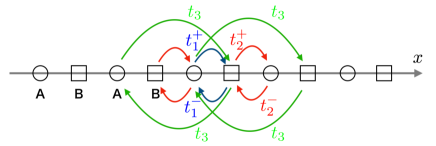
Figure 2: A non-Hermitian extension of the SSH (Su-Schriffer-Heeger) model employed in Refs. Yao and Wang, 2018; Yokomizo and Murakami, 2019. Here, we have updated the convention of $t_{1}^{\pm}$ and $t_{2}^{\pm}$.

II.2 Implementation of the mpbc to a tight-binding model

Let us consider the Hatano-Nelson model Hatano and Nelson (1996, 1997) in the clean limit:

$$H_{HN}=\sum_{x}(t_{R}|x+1\rangle\langle x|+t_{L}|x\rangle\langle x+1|).$$ (5)

The hopping amplitudes $t_{R}$ and $t_{L}$ are chosen to be non-reciprocal: $t_{R}\neq t_{L}$. The recipe for imposing the standard pbc: $\psi(x+L)=\psi(x)$ is well known; one truncates the summation over $x$ in Eq. (5) as

$$H_{HN}^{(L)}=\sum_{x=1}^{L-1}(t_{R}|x+1\rangle\langle x|+t_{L}|x\rangle\langle x+1|).$$ (6)

and adds the boundary term:

$$H_{bd}(1)=t_{R}|1\rangle\langle L|+t_{L}|L\rangle\langle 1|,$$ (7)

which couples the last site ($x=L$) back to the first one ($x=1$) via non-reciprocal hopping terms. The total Hamiltonian $H_{pbc}^{HN}=H_{HN}^{(L)}+H_{bd}(1)$ represents the system under the standard pbc. The eigenstates of $H_{pbc}^{HN}$ take the following standard Bloch form:

$$|\beta\rangle=\sum_{x=1}^{L}\beta^{x}|x\rangle,$$ (8)

with $\beta^{L}=1$, i.e., $|\beta|=1$.

However, Eq. (7) is not a unique choice to make the system periodic by closing it via a boundary hopping term. Instead of Eq. (7), one can equally consider

$$H_{bd}(b)=b^{-L}t_{R}|1\rangle\langle L|+b^{L}t_{L}|L\rangle\langle 1|,$$ (9)

where $b$ is a real positive constant. Imura and Takane (2019) The form of the boundary term (9) implies that the eigenstates of $H_{mpbc}^{HN}(b)=H_{HN}^{(L)}+H_{bd}(b)$ are in the form of Eq. (8) with $\beta$ satisfying $\beta^{L}=b^{L}$, i.e., $|\beta|=b$ or $\beta=be^{ik}$. The eigen wave function $\psi(x)$ satisfies the mpbc:Imura and Takane (2019)

$$\psi(x+L)=b^{L}\psi(x)$$ (10)

At this stage we do not attempt to determine the parameter $b$, but keep it as a free parameter in the theory. For a given $b$, our mpbc specifies that the allowed values of $\beta$ are on a circle of radius $b$ in the complex $\beta$-plane, which represents the generalized Brillouin zone of the system. $b$ can be chosen, for example, as $b=\sqrt{t_{R}/t_{L}}$ representing the degree of skin effect under the obc (see below), but if one’s purpose is simply to restore the bulk-boundary correspondence, it has been shown that such a fine tuning of $b$ is unnecessary except at the bulk gap closing.Imura and Takane (2019)

In an infinite system specified by Eq. (5),

$$|\beta\rangle=\sum_{x}\beta^{x}|x\rangle$$ (11)

with an arbitrary $\beta$ becomes formally an eigenstate of the system, although such a wave function is generally unbounded and not compatible with quantum mechanics. The corresponding eigenenergy $E(\beta)$ is determined as

$$t_{R}\beta^{-1}+t_{L}\beta=E=E(\beta).$$ (12)

From these infinite number of eigenstates, the boundary Hamiltonian (9) selects those solutions satisfying $\beta^{L}=b^{L}$. As for the standard pbc, it selects only those solutions with $\beta^{L}=1$. This turns out to be too restrictive and inadequate for a description of the bulk in the bulk-boundary correspondence.

Let us comment on the obc case, in which the Schrödinger equation is $H_{HN}^{(L)}|\psi_{obc}\rangle=E|\psi_{obc}\rangle$ with $|\psi_{obc}\rangle=\sum_{x}\psi_{obc}(x)|x\rangle$. The wave function $\psi_{obc}(x)$ subjected to the boundary condition of $\psi_{obc}(0)=0$ is expressed as a superposition of the generalized Bloch form (8):

$$\psi_{obc}(x)\propto\beta_{1}^{x}-\beta_{2}^{x},$$ (13)

where $\beta_{1}$ and $\beta_{2}$ are the two solutions of Eq. (12) at an equal energy $E$, which implies $\beta_{1}\beta_{2}=t_{R}/t_{L}\neq 1$. We also need to impose the boundary condition: $\psi_{obc}(L+1)=0$. This enforces

$$(\beta_{1}/\beta_{2})^{L+1}=1,$$ (14)

implying together with the previous condition, $|\beta_{1}|=|\beta_{2}|=\sqrt{t_{R}/t_{L}}\neq 1$. As a result $\psi_{obc}(x)$ tends to damp or amplify exponentially towards the end of the system (non-Hermitian skin effect).Yao and Wang (2018)

III A non-Hermitian SSH model

We present a non-Hermitian extension of the Su-Schriffer-Heeger (SSH) model Su et al. (1979) (see Fig. 2), which is used to illustrate our scenario in subsequent sections. Among different extensions Lieu (2018) we consider here a variation with non-reciprocal hopping, since this type of non-Hermiticity is more problematic for the bulk-boundary correspondence than the complex potentials (gain/loss type non-Hermiticity). Lee (2016); Song et al. (2019); Zirnstein et al. (2019); Lee and Thomale (2019); Yao and Wang (2018); Yokomizo and Murakami (2019)

III.1 The model

A non-Hermitian version of the SSH model:

$$H_{\rm NN}^{(L)} = \sum_{x=1}^{L}\left[t_{1}^{+}|x,B\rangle\langle x,A|+t_{1}^{-}|x,A\rangle\langle x,B|\right]$$ (15)

$$+ \sum_{x=1}^{L-1}\left[t_{2}^{+}|x+1,A\rangle\langle x,B|+t_{2}^{-}|x,B\rangle\langle x+1,A|\right],$$

gives a prototypical example, in which one encounters the difficulty of applying the standard pbc to a non-Hermitian system. Lee (2016) The nearest-neighbor (NN) hopping amplitudes:

$$t_{1}^{\pm}=t_{1}\pm\gamma_{1},\ \ t_{2}^{\pm}=t_{2}\pm\gamma_{2},$$ (16)

are chosen to be non-reciprocal. $t_{1}^{\pm}$ represents an intra-cell hopping amplitudes in the $\pm x$ direction. $t_{2}^{\pm}$ represents an inter-cell hopping amplitudes in the $\pm x$ direction. Here, following Refs. Yao and Wang, 2018; Yokomizo and Murakami, 2019 we also consider third-nearest-neighbor (3NN) hopping terms $t_{3}$ such that

$$H_{\rm 3NN}^{(L)}=\sum_{x=1}^{L-1}\left[t_{3}|x+1,B\rangle\langle x,A|+t_{3}|x,A\rangle\langle x+1,B|\right].$$ (17)

Our total Hamiltonian reads

$$H_{\rm SSH}^{(L)} = H_{\rm NN}^{(L)}+H_{\rm 3NN}^{(L)}.$$ (18)

We assume that the model parameters $t_{\mu}(\mu=1,2,3)$, $\gamma_{\mu}(\mu=1,2)$ are all real constants. The Hamiltonian (18) with Eqs. (15) and (17) describes our system under the obc.

III.2 The mpbc: the boundary Hamiltonian and the generalized Bloch Hamiltonian

To discuss bulk-boundary correspondence in the non-Hermitian SSH model (18) we need to consider it in a bulk geometry. This is realized by introducing boundary hopping terms that close the system. We introduce boundary terms that concretize the mpbc, which have NN and 3NN parts:

$$H_{bd}^{\rm SSH}(b)=H_{bd}^{\rm NN}(b)+H_{bd}^{\rm 3NN}(b),$$ (19)

where

$$H_{bd}^{\rm NN}(b) = b^{-L}t_{2}^{+}|1,A\rangle\langle L,B|+b^{L}t_{2}^{-}|L,B\rangle\langle 1,A|,$$

$$H_{bd}^{\rm 3NN}(b) = b^{-L}t_{3}|1,B\rangle\langle L,A|+b^{L}t_{3}|L,A\rangle\langle 1,B|.$$ (20)

These hopping matrix elements couple the final unit cell $x=L$ back to the first one $x=1$ (and vice versa), with an amplitude amplification ($b^{L}$) or attenuation ($b^{-L}$) factor to select eigenstates of an appropriate amplitude $b$ (see Sec. II). Note also that the boundary Hamiltonian (20) is non-Hermitian unless $b=1$. The total Hamiltonian under the mpbc reads

$$H_{mpbc}^{\rm SSH}(b)=H_{\rm SSH}^{(L)}+H_{bd}^{\rm SSH}(b).$$ (21)

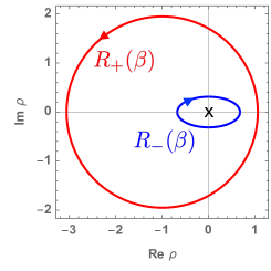
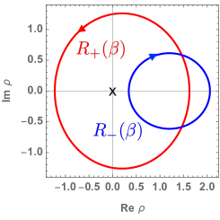
(a) (b) (c)

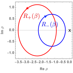
Figure 3: The trajectory of $\rho_{\pm}=R_{\pm}(\beta)$ [cf. Eq. (40)] at different points in Fig. 1 with $t_{2}=1$, $t_{3}=0.1$, $\gamma_{1}=0.5$, $\gamma_{2}=0.1$, where $\times$ indicates the position of origin. Panel (a): $(t_{1},b)=(-0.5,0.7)$ in the $R$ region (TI phase) with $(w_{+},w_{-})=(1,-1)$ and $w=1$. Panel (b): $(t_{1},b)=(0.6,0.2)$ in the $G_{1}$ region with $(w_{+},w_{-})=(1,0)$ and $w=1/2$. Panel (c): $(t_{1},b)=(-1.7,0.1)$ in the $B_{1}$ region (OI phase) with $(w_{+},w_{-})=(0,0)$ and $w=0$.

As in the single-band case, the eigenstate of $H_{mpbc}^{\rm SSH}(b)$ takes a generalized Bloch form:

$$|\beta\rangle=\sum_{x=1}^{L}\beta^{x}(u_{A}|x,A\rangle+u_{B}|x,B\rangle),$$ (22)

where $\beta^{L}=b^{L}$, i.e., $\beta=be^{ik}$ with $k=2\pi n/L$, $n=0,1,2,\cdots,L-1$. Such values of $\beta$ are on a circle of radius $b$ in the complex $\beta$-plane, which represents our generalized Brillouin zone in the limit of $L\rightarrow\infty$. Equation (22) is a two-band generalization of Eq. (8). Then, the eigenvalue problem:

$$H_{mpbc}^{\rm SSH}|\beta\rangle=E(\beta)|\beta\rangle,$$ (23)

reduces to the following $2\times 2$ problem specified by the generalized Bloch Hamiltonian $H_{mpbc}(\beta)$:

$$H_{mpbc}(\beta)\left[\begin{array}[]{c}u_{A}\\ u_{B}\end{array}\right]=E(\beta)\left[\begin{array}[]{c}u_{A}\\ u_{B}\end{array}\right],$$ (28)

where

$$H_{mpbc}(\beta)=\left[\begin{array}[]{cc}0&R_{-}(\beta)\\ R_{+}(\beta)&0\end{array}\right],$$ (29)

and

$$R_{+}(\beta) = t_{1}^{+}+t_{2}^{-}\beta+t_{3}\beta^{-1},$$

$$R_{-}(\beta) = t_{1}^{-}+t_{2}^{+}\beta^{-1}+t_{3}\beta.$$ (30)

Note that $H_{mpbc}(\beta)$ is chiral (sublattice Kawabata et al. (2019)) symmetric so that our system belongs to class AIII. Kawabata et al. (2019); Kitaev et al. (2009); Schnyder et al. (2008); Ryu et al. (2010)

For a given $\beta=be^{ik}$ the corresponding energy eigenvalue $E(\beta)$ is determined by the secular equation:

$$R_{+}(\beta)R_{-}(\beta)=E^{2},$$ (31)

which is a quartic equation for $\beta$ in the present case. Note that generally $E$ is complex.

III.3 Case of the obc

To achieve the bulk-boundary correspondence in the present model one needs to consider also its boundary geometry.Ryu and Hatsugai (2002); Imura and Takane (2019) The boundary geometry is realized by imposing the obc. As noted before, this is equivalent to consider $H_{\rm SSH}^{(L)}$ as the total Hamiltonian of the system. Thus by diagonalizing $H_{\rm SSH}^{(L)}$ one finds the obc spectrum. When the model parameters are those corresponding to the topologically nontrivial phase [topological insulator (TI) phase], one finds a pair of boundary states at $E=0$ in the spectrum. The rest of the spectrum forms asymptotically a bulk energy band in the limit of $L\rightarrow\infty$. If $E$ falls on the bulk energy band, the corresponding eigenstate $|E_{obc}\rangle$ under the obc must have the following characteristics.Yokomizo and Murakami (2019); Yao and Wang (2018)

In the present model the secular equation (31) is quartic so that for a given $E$ there are four solutions $\beta_{j}$s ($j=1,2,3,4$) for $\beta$. Unlike under the mpbc, the amplitudes $|\beta|$ are not a priori specified quantities. We label $\beta_{j}$s in the increasing order of their magnitude such that

$$|\beta_{1}|\leq|\beta_{2}|\leq|\beta_{3}|\leq|\beta_{4}|.$$ (32)

The eigenstate $|E_{obc}\rangle$ under the obc can be expressed as a superposition of four fundamental solutions such that

$$|E_{obc}\rangle=c_{1}|\beta_{1}\rangle+c_{2}|\beta_{2}\rangle+c_{3}|\beta_{3}\rangle+c_{4}|\beta_{4}\rangle,$$ (33)

where $|\beta_{j}\rangle$s are given as

$$|\beta_{j}\rangle=\sum_{x}\beta_{j}^{x}(u_{A}|x,A\rangle+u_{B}|x,B\rangle)$$ (34)

for $j=1,2,3,4$. Each $|\beta_{j}\rangle$ is a fundamental solution of the infinite system and not an eigenstate compatible with the obc. The two central components of Eq. (33) are analogues of the plane-wave components $e^{ikx}$ and $e^{-ikx}$ in the Hermitian case, while the other components associated with $\beta_{1}$ and $\beta_{4}$ are sorts of evanescent modes to make the function to be compatible with the obc. For the wave function (33) to be an eigenstate in the bulk energy band under the obc, $|\beta_{2}\rangle$ and $|\beta_{3}\rangle$ must satisfyYao and Wang (2018); Yokomizo and Murakami (2019)

$$|\beta_{2}|=|\beta_{3}|$$ (35)

in the limit of $L\rightarrow\infty$. This condition, in turn, determines the allowed values of $E$ forming the bulk energy band. The trajectory of $\beta_{2}$ or $\beta_{3}$ satisfying Eq. (35) defines the generalized Brillouin zone of this obc approach.Yao and Wang (2018); Yokomizo and Murakami (2019) Note that under the mpbc we employ a different generalized Brillouin zone.

IV Non-Hermitian winding numbers

As noted earlier our one-dimensional model is chiral symmetric. In the Hermitian limit, it is well established that such a system is classified by a $\mathbb{Z}$-type topological number, or a winding number. Kitaev et al. (2009); Schnyder et al. (2008); Ryu et al. (2010)

IV.1 A pair of non-Hermitian chiral winding numbers

Extrapolating our knowledge in the Hermitian limit, let us consider the following pair of chiral winding numbers defined in the bulk geometry under the mpbc:

$$w_{\pm}(b) = {1\over 2\pi}[\arg R_{\pm}(\beta)]_{k=0}^{2\pi}$$ (36)

$$= {1\over 2\pi}[\phi_{\pm}(2\pi)-\phi_{\pm}(0)],$$

where $\beta=be^{ik}$, $R_{\pm}$ are given in Eqs. (30), and

$$\phi_{\pm}(k)={\rm Im}\log R_{\pm}(\beta).$$ (37)

Here, for $k$ to be continuous, the limit $L\rightarrow\infty$ is implicit. The winding numbers $w_{\pm}(b)$ are functions of model parameters $t_{\mu}$, $\gamma_{\mu}$ and also of $b$ specifying the mpbc. In this sense $w_{\pm}$ are defined in the generalized parameter space

$$\tilde{\tau}=\{b,\tau\},$$ (38)

where

$$\tau=\{t_{\mu},\gamma_{\mu}\}$$ (39)

is the original set of parameters. $w_{\pm}$ measures how many times the trajectory,

$$\rho=R_{\pm}(\beta)\equiv\rho_{\pm}$$ (40)

winds around the origin in the complex $\rho$-plane while $\beta=be^{ik}$ goes around the generalized Brillouin zone once in the anti-clockwise direction (while $k$ sweeps the standard BZ: $k\in[0,2\pi]$ once from 0 to $2\pi$). The three panels of Fig. 3 represent the trajectory $\rho_{\pm}(t_{1},b)$ at different points in Fig. 1 (the winding number map).

In the Hermitian limit: $\gamma_{1}=\gamma_{2}=0$, $b=1$, the Hermiticity requires $R_{-}=R_{+}^{*}$, so that $w_{-}$ is fixed to $-w_{+}$. The winding number $w$ is defined as

$$w\equiv{w_{+}-w_{-}\over 2}=w_{+}=-w_{-}.$$ (41)

It is well established that $w=1$ encodes the existence of a pair of boundary states at $E=0$ (TI phase), while $w=0$ encodes the absence of boundary states [ordinary insulator (OI) phase], giving a prototypical example of the bulk-boundary correspondence.

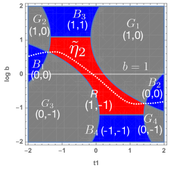
(a) (b) (c)

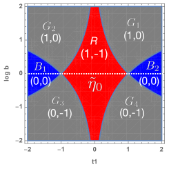
Figure 4: Evolution of the path $\tilde{\eta}$ in the perturbative non-Hermitian regime. Panel (a) describes a situation analogous to the one in Fig. 1 (non-Hermiticity is slightly strong): $t_{2}=1$, $t_{3}=0.05$, $\gamma_{1}=0.75$, $\gamma_{2}=0.1$. Panel (c) describes the Hermitian limit: $t_{2}=1$, $t_{3}=\gamma_{1}=\gamma_{2}=0$. Panel (b) corresponds to an intermediate situation with $t_{2}=1$, $t_{3}=0.05$, $\gamma_{1}=0.2$, $\gamma_{2}=0.05$. The path $\tilde{\eta}$ evolves as $\tilde{\eta}_{2}\rightarrow\tilde{\eta}_{1}\rightarrow\tilde{\eta}_{0}$. In each topologically distinct region the value of $(w_{+},w_{-})$ is given.

IV.2 The phase diagram in the bulk geometry

Away from the Hermitian limit, the pair of winding numbers $(w_{+},w_{-})$ specifies topologically distinct regions in $\tilde{\tau}$, each of which represents a gapped topological phase. In Fig. 1(b), different gapped phases in the bulk geometry under the mpbc are shown in the subspace $\{t_{1},b\}$ of $\tilde{\tau}$, and specified by $w_{\pm}(t_{1},b)$.

The phase boundaries of such a winding number map are given by the gap closings under the mpbc (see Fig.1 as an example). At the gap closings, the quartic equation (31) with $E=0$ must hold and gives four solutions of $\beta=be^{ik}$, which are expressed as $\beta=\beta_{\mu}$ ($\mu=1,2,3,4$). This indicates that a solution with $E=0$ appears under the mpbc if $b=b_{\mu}(t_{1})$ ($\mu=1,2,3,4$), where $b_{\mu}=|\beta_{\mu}|$. That is, each trajectry $b=b_{\mu}(t_{1})$ ($\mu=1,2,3,4$), on which the gap closes, serves as a phase boundary. At $E=0$, Eq. (31) reduces to a set of decoupled equations: $R_{+}(\beta)=0$ and $R_{-}(\beta)=0$. Therefore, two of the four $\beta_{\mu}$s are the solutions of $R_{+}(\beta)=0$, and the other two are those of $R_{-}(\beta)=0$. Thus, on a phase boundary: $b=b_{\mu}$, either of the trajectory $R_{\pm}(\beta=b_{\mu}e^{ik})$ passes the origin at $\beta=\beta_{\mu}$. Therefore, at this point $w_{\pm}$ changes by $\pm 1$.

Note that the gap closings under the mpbc (the phase boundaries: $b=b_{\mu}$), generally, do not correspond to any physical reality in the boundary geometry under the obc as explained in the next section.

V Generalized bulk-boundary correspondence: the prescription

In the previous section, we have seen how a pair of winding numbers $(w_{+},w_{-})$ classifies different gapped phases in the bulk geometry. Here, we discuss how this could be related to the physical reality in the boundary geometry under the obc (bulk-boundary correspondence). Below we give a prescription how to establish a one-to-one relation between the presence/absence of boundary states under the obc and $(w_{+},w_{-})$ under the mpbc.

V.1 $P$ and $\tilde{P}$ are corresponding

To specify a boundary geometry under the obc, one needs to specify a point $P$ in $\tau$. At a given point $P$ one has a concrete obc spectrum such as the one represented in Fig. 1 (a) [top annex panel]. At $P$ one can tell from the obc spectrum whether the system is in the TI phase: a pair of zero-energy boundary states, or in the OI phase: no boundary state.

To define a bulk geometry, one needs to specify also the mpbc parameter $b$; defining a bulk geometry is thus equivalent to specifying a point $\tilde{P}$ in $\tilde{\tau}$ corresponding to $P$. To establish the bulk-boundary correspondence the value of $b$ must be specified at an arbitrary point $P$ in such a way that the boundary property is always in one-to-one correspondence with $(w_{+},w_{-})$ at $\tilde{P}$.

In the obc spectrum shown in Fig. 1 (a) one can follow how the boundary property at $P$ evolves as $t_{1}$ is varied. In the subspace considered in Fig. 1, $P=t_{1}$, and the corresponding point $\tilde{P}$ can be denoted as $\tilde{P}=(t_{1},b)$. The pair of winding numbers $(w_{+},w_{-})$ at an arbitrary point $\tilde{P}$ is given in Fig. 1. To complete our recipe for achieving the bulk-boundary correspondence, the function $b=b(t_{1})$ must be given which specifies a path $\tilde{\eta}$ that the point $\tilde{P}$ follows in (the subspace of) $\tilde{\tau}$.

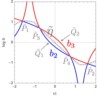
(a) (b)

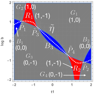
Figure 5: The trajectories of $b_{2}$ and $b_{3}$ [panel (a)] and the corresponding winding number map [panel (b)] in the non-perturbative non-Hermitian regime. Parameters: $t_{2}=1$, $t_{3}=0$, $\gamma_{1}=1.25$, $\gamma_{2}=0$.

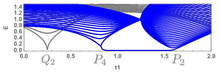
Figure 6: The obc (pbc) spectrum [shown in blue (gray)] corresponding to Fig. 5. Only the $t_{1}>0$ part is shown. A pair of zero-energy end states appears between the points $P_{4}$ and $P_{2}$, corresponding, respectively, to $\tilde{P}_{4}$ and $\tilde{P}_{2}$ in Fig. 5. The path $\tilde{\eta}$ is in the TI region $R2$ in this range of $t_{1}$.

V.2 Perturbative non-Hermitian regime

In the Hermitian limit: $\gamma_{1}=\gamma_{2}=0$, the bulk-boundary correspondence is done by smooth deformation of the model parameters so as not to change the winding number $w$.Ryu and Hatsugai (2002) The model parameters in the TI region with boundary states can be smoothly reduced to $t_{1}=0$, $t_{2}=1$ and $t_{3}=0$ with keeping $w=1$. Those in the OI region with no boundary state can be reduced to $t_{1}=1$, $t_{2}=0$ and $t_{3}=0$ with keeping $w=0$. In the non-Hermitian case we do the same kind of smooth deformation in $\tilde{\tau}$.Imura and Takane (2019)

We consider the perturbative non-Hermitian regime, in which the arrangement of TI and OI phases in the boundary geometry is identical to the one in the Hermitian limit, i.e., only the position of the phase boundaries differs from the Hermitian limit. Let us define $\tilde{\eta}_{0}$ as the trajectory of $\tilde{P}$ in the Hermitian limit. Namely, $\tilde{\eta}_{0}=(t_{1},b=1)$. An example is shown in Fig. 4(c). Note that $\tilde{\eta}_{0}$ goes through all the crossing points of $b_{2}$ and $b_{3}$ and apart from these points it stays in a region sandwiched between $b_{2}$ and $b_{3}$; i.e.,

$$b_{2}(t_{1})<b(t_{1})=1<b_{3}(t_{1}).$$ (42)

If $\tilde{\eta}$ is smoothly connected to $\tilde{\eta}_{0}$, the bulk-boundary correspondence is at work. By $\tilde{\eta}$ being smoothly connected to $\tilde{\eta}_{0}$, we mean that the arrangement of $(w_{+},w_{-})$ on $\tilde{\eta}$ must be the same as the ones on $\tilde{\eta}_{0}$.

In considering $\tilde{\eta}$, it is useful to note the following. As $t_{1}$ varies, $P=t_{1}$ experiences different gapped phases (TI, or OI) in the boundary geometry (see Fig. 1). Bulk energy gap closes at the phase boundary between neighboring gapped phases. We name such phase boundaries as $P_{j}$s ($j=1,2,\cdots$) with $P_{j}=t_{1}^{(j)}$. Then, the two trajectories $b_{2}(t_{1})$ and $b_{3}(t_{1})$ cross at $t_{1}=t_{1}^{(j)}$, and this must be always the case. The reason is the following. As the bulk gap closes in the boundary geometry at $P_{j}=t_{1}^{(j)}$, there must exist a zero-energy solution in the form of Eq. (33). This combined with Eq. (35) requires that Eq. (31) with $E=0$ gives $\beta_{\mu}$s satisfying

$$|\beta_{1}(t_{1}^{(j)})|<|\beta_{2}(t_{1}^{(j)})|=|\beta_{3}(t_{1}^{(j)})|<|\beta_{4}(t_{1}^{(j)})|.$$ (43)

Note that the secular equation is independent of a boundary condition. Combining Eq. (43) with the definition of $b_{\mu}(t_{1})$ in the bulk geometry (i.e., $b_{\mu}(t_{1})=|\beta_{\mu}(t_{1})|$ with $\beta_{\mu}(t_{1})$s being solutions of the secular equation at $E=0$), we readily find $b_{2}(t_{1}^{(j)})=b_{3}(t_{1}^{(j)})$. This indicates that $b_{2}(t_{1})$ and $b_{3}(t_{1})$ must cross at $t_{1}=t_{1}^{(j)}$.

As $\tilde{\eta}_{0}$ goes through all the crossing points of $b_{2}$ and $b_{3}$, $\tilde{\eta}$ must go through all the corresponding points in order to be smoothly connected to $\tilde{\eta}_{0}$. That is, the crossing point of $b_{2}(t_{1})$ and $b_{3}(t_{1})$ at $t_{1}=t_{1}^{(j)}$ should be identified as $\tilde{P}_{j}$ corresponding to $P_{j}$. Apart from $\tilde{P}_{j}$s, $\tilde{\eta}$ is not allowed to cross any of the trajectory of $b_{\mu}$. If it does, the bulk spectrum becomes gapless, while the obc spectrum remains gapped as the bulk condition (35) is unsatisfied at the corresponding point in $\tau$.

In consequence, the condition for $\tilde{\eta}$ is given as follows:

1. $\tilde{\eta}$ must go through all the crossing points of $b_{2}$ and $b_{3}$.

2. Apart from these points it must stay in a region sandwiched between the two trajectories $b_{2}$ and $b_{3}$:

   $$b_{2}(t_{1})<b(t_{1})<b_{3}(t_{1}).$$ (44)

Figure 4 shows how such a smooth deformation is done in $\tilde{\tau}$. $\tilde{\eta}_{2}$ in panel (a) is smoothly deformed to $\tilde{\eta}_{1}$ in panel (b), then to $\tilde{\eta}_{0}$ in the Hermitian limit [panel (c)]. Note also that away from the crossing points $\tilde{P}_{j}$, the choice of $\tilde{\eta}$ is not unique.

In Figs. 1 and 4 the gray regions with $w=1/2$, corresponding to $(w_{+},w_{-})=(1,0),(0,-1)$, are new topologically distinct regions absent in the Hermitian limit. The above argument shows that $\tilde{\eta}$ does not pass either of such a region. Thus, the new topological region with $w=1/2$ will not manifest any physical reality under the obc.

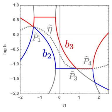
(a) (b)

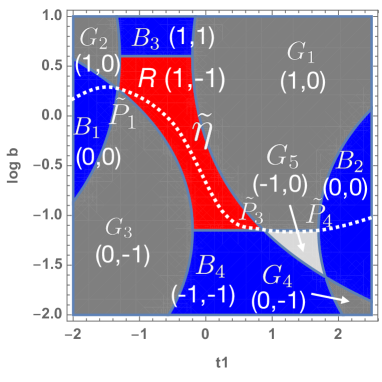
Figure 7: Case of a finite gapless region (non-perturbative non-Hermitian regime). Parameters: $t_{2}=1$, $t_{3}=0.15$, $\gamma_{1}=0.75$, $\gamma_{2}=0.5$.

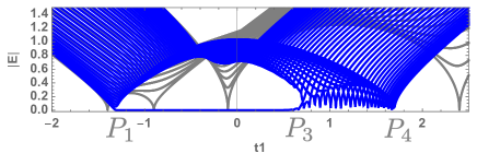
Figure 8: The obc (pbc) spectrum [shown in blue (gray)] corresponding to Fig. 7. The bulk part of the spectrum is expected to be gapless in a finite range of $t_{1}$ between $P_{3}$ and $P_{4}$, corresponding, respectively, to $\tilde{P}_{3}$ and $\tilde{P}_{4}$ in Fig. 7.

In our previous argument Imura and Takane (2019) we proposed that $\tilde{\eta}$ must be chosen to be smoothly connected to $\tilde{\eta}_{0}$. Here, we show that this is equivalent to choosing $\tilde{\eta}$ to satisfy the inequality (44). Below this new recipe is applied to a non-perturbative non-Hermitian regime.

V.3 Non-perturbative non-Hermitian regime

Let us next consider the non-perturbative non-Hermitian regime, in which non-Hermiticity is strong enough to induce a new distinct gapped phase absent in the Hermitian limit. When such a new gapped phase is present in the boundary geometry, $\tilde{\eta}$ in the bulk geometry cannot be smoothly connected to $\tilde{\eta}_{0}$. However, if one requires the same condition as in the perturbative regime to $\tilde{\eta}$ [cf. the inequality (44)], the bulk-boundary correspondence is also at work in the same way. This is almost trivial if one notices the continuity of $\tilde{\eta}$ as a curve before and after the appearance of the new gapped phase. Note that the change of the arrangement of $(w_{+},w_{-})$ on $\tilde{\eta}$ becomes discontinuous in this regime.

The phase diagram shown in Fig. 5 represents an example of such a parameter region. The appearance of the central OI region $B_{3}$ with split TI regions $R_{1}$ and $R_{2}$ [see panel (b)] is the new feature absent in the Hermitian limit. The appearance of $B_{3}$ leads to additional crossing points of $b_{2}$ and $b_{3}$ ($\tilde{P}_{3}$ and $\tilde{P}_{4}$). The inequality (44) suggests that $\tilde{\eta}$ goes through these crossing points. Again, only at these points $\tilde{P}_{3}$ and $\tilde{P}_{4}$, the OI region $B_{3}$ touches either of the two TI regions.

The path $\tilde{\eta}$ incident in the TI region $R_{1}$ goes through $\tilde{P}_{3}$, enters the OI region $B_{3}$, going through $\tilde{P}_{4}$, arrives at the TI region $R_{2}$, then follows the original (perturbative) track. Between $\tilde{P}_{3}$ and $\tilde{P}_{4}$, $\tilde{\eta}$ must go through the OI region $B_{3}$ without touching or crossing $b_{2}$ or $b_{3}$, but must stay in between. At any moment, $\tilde{\eta}$ is not allowed to enter either of the gray region: $G_{1}$ or $G_{3}$.

In this case $\tilde{\eta}$ is not smoothly connected to $\tilde{\eta}_{0}$, but the correspondence to the obc spectrum is still maintained. Figure 6 represents an obc spectrum (shown in blue) corresponding to Fig. 5, where the $t_{1}>0$ part of the spectrum is shown. The gapped region at small $t_{1}$ corresponds to the OI region $B_{3}$. As $t_{1}$ is increased, a pair of zero-energy end states appear between $P_{4}$ and $P_{2}$, corresponding to the TI region $R_{2}$. One can thus verify that the additional crossing point $\tilde{P}_{4}$ corresponds to a new gap closing $P_{4}$.

V.4 Finite gapless region

Finally, let us consider a parameter region employed in Fig. 7. In this region, another feature absent in the Hermitian limit becomes possible: the degeneracy of $b_{2}$ and $b_{3}$ [the condition (43)] maintained in a finite region of $t_{1}$ between $\tilde{P}_{3}$ and $\tilde{P}_{4}$. The path $\tilde{\eta}$ incident in the TI region $R$ with $(w_{+},w_{-})=(1,-1)$ goes through this infinitely narrow path $\tilde{P}_{3}\tilde{P}_{4}$ to enter the OI region $B_{2}$. Under the obc (Fig. 8) the path $\tilde{P}_{3}\tilde{P}_{4}$ corresponds to a quasi-gapless region between $P_{3}$ and $P_{4}$.Yokomizo and Murakami (2019) In the limit $L\rightarrow\infty$, the spectrum is expected to become gapless in this finite segment $P_{3}P_{4}$. The corresponding path $\tilde{P}_{3}\tilde{P}_{4}$ is characterized as the phase boundary between the half-integral $w$ regions in the bulk geometry: $G_{1}$ and $G_{5}$ (the gray and light-gray regions). $G_{5}$ is a newly emerged region with $w=-1/2$, $(w_{+},w_{-})=(-1,0)$, distinct from $G_{1}$ with $w=1/2$, $(w_{+},w_{-})=(1,0)$.

VI Conclusions

Motivated by the newly proposed non-Hermitian topological insulator, we have developed non-Hermitian Bloch band theory. The concept of bulk-boundary correspondence is the central idea of topological insulator, while in some non-Hermitian models with non-reciprocal hopping this correspondence is superficially broken. In such non-Hermitian systems due to the non-Hermitian skin effect, the bulk spectrum is somewhat too sensitive to a boundary condition for the standard procedure to be valid as such.

We have proposed to employ the modified periodic boundary condition (mpbc) for describing the bulk of such a system. The use of this mpbc appropriately captures the features specific to non-Hermitian systems, and underlies the Bloch band theory for non-Hermitian systems. We have shown that the bulk-boundary correspondence is restored in the generalized parameter space $\tilde{\tau}=\{\tau,b\}$, where $\tau$ represents the original model parameter space, and $b$ specifies the mpbc.

In the generalized bulk-boundary correspondence, a pair of chiral winding numbers $(w_{+},w_{-})$ evaluated on the path $\tilde{\eta}$ in $\tilde{\tau}$ plays the role of characterizing each topologically distinct region. We present a simple recipe to give $\tilde{\eta}$ in a proper manner.

To illustrate our scenario we have employed a non-Hermitian version of the SSH model. However, the proposed scenario itself should be applicable to a broader class of non-Hermitian topological insulators. A relation analogous to Eq. (44) can be equally found for a different class of models, e.g., for models with symplectic symmetry. Kawabata et al. (2020); Okuma et al. (2020) In such cases the concrete relation (44) should be replaced with a suitable one, but the rest of the recipe is unchanged. Restoring the bulk-boundary correspondence in its proper sense as a correspondence between the genuine bulk and boundary quantities, our generalized Bloch band theory set the basis on which the concept of topological insulator is firmly established in non-Hermitian systems.