A Higher-order Trace Finite Element Method for Shells

Abstract

A higher-order fictitious domain method (FDM) for Reissner-Mindlin shells is proposed which uses a three-dimensional background mesh for the discretization. The midsurface of the shell is immersed into the higher-order background mesh and the geometry is implied by level-set functions. The mechanical model is based on the Tangential Differential Calculus (TDC) which extends the classical models based on curvilinear coordinates to implicit geometries. The shell model is described by PDEs on manifolds and the resulting FDM may typically be called Trace FEM. The three standard key aspects of FDMs have to be addressed in the Trace FEM as well to allow for a higher-order accurate method: (i) numerical integration in the cut background elements, (ii) stabilization of awkward cut situations and elimination of linear dependencies, and (iii) enforcement of boundary conditions using Nitsche’s method. The numerical results confirm that higher-order accurate results are enabled by the proposed method provided that the solutions are sufficiently smooth.

Keywords: Trace FEM; Fictitious domain methods; Tangential differential calculus; Shells; Manifolds; Level-Set method; Implicit geometries;

1 Introduction

A shell is a curved, thin-walled structure and due to their high bearing capacity, they occur in many engineering applications such as automotive, aerospace, biomedical- and civil-engineering [12, 22, 59]. In the mechanical modelling of a shell, a dimensional reduction from the 3D shell body to its midsurface is a key step. The equilibrium equations result into partial differential equations (PDEs) on manifolds embedded in the physical space $\mathbb{R}^{3}$. In the classical approach of modelling shells, the midsurface is typically defined by a (piecewise) parametrization which may be called an explicit definition. Then, there exists a map from some two-dimensional parameter space $\hat{\Omega}$ to $\mathbb{R}^{3}$. In the context of the classical Surface FEM, the discrete midsurface is rather defined by an atlas of local element-wise mappings from the reference element to the physical elements. An overview of classical shell theory is given, e.g., in [15, 56, 57, 3] or in the text books [12, 4, 1, 58, 59]. Alternatively, the shell geometry may also be defined implicitly following the level-set method [25, 26, 48, 55]. The main advantage of implicit geometry descriptions is that the application of recent finite element techniques such as fictitious domain methods (FDM) for shells is enabled.

Herein, we propose a higher-order accurate fictitious domain method for implicitly defined Reissner–Mindlin shells. The geometry of the shell is defined implicitly by means of level-set functions. The shell boundary value problem (BVP) is discretized with a higher-order accurate Trace FEM approach.

The Trace FEM is a fictitious domain method for solving PDEs on manifolds, see, e.g., [49, 44, 45, 31, 29, 54, 5]. This may also be called Cut FEM which, in the last years, became a popular FDM enabling higher-order accuracy [8, 10, 9]. When using the Cut FEM for the solution of PDEs on manifolds as done herein, the method becomes analogous to the Trace FEM [11, 13]. This recent finite element technique is fundamentally different compared to standard Surface FEM approaches, see, e.g., [19, 21, 23, 26]. In the following, the major differences in, (1) geometry definition, (2) mesh and degrees of freedom (DOFs) and, (3) generation of integration points in these two approaches are outlined and visualized for the Trace FEM in Fig. 1 and for the Surface FEM in Fig. 2, respectively.

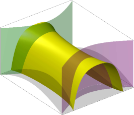
((a)) implicit shell midsurface

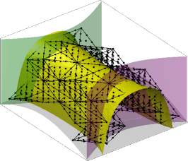
((b)) cut elements

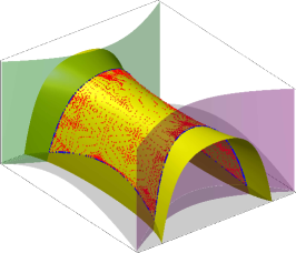
((c)) integration points on the zero-isosurface

Fig. 1: Overview of the Trace FEM: (a) Implicit definition of the shell geometry by means of level-set functions, (b) the set of cut three-dimensional background elements are labelled as active mesh and their nodes imply the DOFs for the numerical simulation, (c) integration points on the zero-isosurface plotted in red for the domain and in blue on the boundary.

((a)) explicit shell midsurface

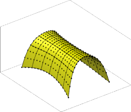
((b)) surface mesh

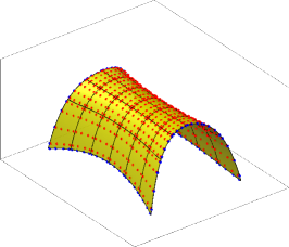
((c)) integration points on the surface mesh

Fig. 2: Overview of the Surface FEM: (a) Explicitly defined shell obtained by an atlas of element-wise local mappings, (b) conforming surface mesh consisting of cubic 2D Lagrange elements, (c) integration points for the Surface FEM obtained by standard Gauß integration rules.

1. Firstly, the differences in the geometry definition are emphasized. In Fig. 1(a), an implicitly defined shell by means of level-set functions is presented. In particular, the yellow surface indicates the midsurface of the shell and is defined by the zero-isosurface of a master level-set function. The boundary of the shell is defined by additional slave level-set functions, i.e., the light green, purple and grey surfaces in Fig. 1(a). In contrast to the implicit definition, an explicit representation of the shell midsurface for this example is shown in Fig. 2(a). Then, the surface is given through an atlas of element-wise local mappings, as usual in the context of Surface FEM, implying local curvilinear coordinates. Note that a parametrization is only available in the explicit case and is, in general, not available in implicitly defined geometries.

2. Secondly, the mesh generation and the location of DOFs are considered. In the Trace FEM the domain of interest, i.e., the shell midsurface, is embedded in a three-dimensional background mesh. The 3D background mesh may consist of higher-order Lagrange elements with the only requirement that the domain of interest is completely immersed. Neither the shell surface nor the shell boundary have to conform to the background mesh. There is one master level-set function whose zero-isosurface implies the shell surface and additional slave level-set functions imply the boundaries. The set of cut elements is labelled active mesh and is visualized in Fig. 1(b) where cubic tetrahedral elements are used as an example. For the numerical simulation, the DOFs are located at the nodes of the active mesh, which are clearly not on the midsurface of the shell. The corresponding shape functions are those of the active mesh and are restricted to the trace. This means that for the integration of the weak form, the 3D shape functions are only evaluated on the zero-isosurface of the master level-set function. In contrast, in the Surface FEM a boundary conforming surface mesh, see Fig. 2(b), is defined through an atlas of element-wise local mappings and the DOFs are located at nodes of the surface mesh which are on the discrete midsurface of the shell. The corresponding shape functions are the 2D shape functions living only on the surface mesh. The location of the DOFs and the different dimensionality of the shape functions are the most important differences between the two finite element techniques.

3. Lastly, integration points need to be placed on the shell midsurface for the integration of the weak form. In the case of the Trace FEM, this is not a trivial task especially when a higher-order accurate integration scheme is desired [24, 25, 26, 27, 42, 40], further details are given below. Regarding the Surface FEM standard Gauß integration rules are applicable and mapped from the reference to the surface elements in the usual manner. In Fig. 1(c) and Fig. 2(c), integration points in the domain (red) and on the boundary (blue) are visualized for the Trace FEM and Surface FEM, respectively.

As mentioned above, the Trace FEM approach is a fictitious domain method and the following three well-known implementational aspects require special attention: (i) integration of the weak form, (ii) stabilization and, (iii) enforcement of essential boundary conditions. Regarding the integration of the weak form, suitable integration points with higher-order accuracy for multiple level-set functions have to be provided. Herein, the approach, which naturally extends to multiple level-set functions as outlined by the authors in [24, 25, 26, 27] is employed. Other higher-order integration schemes for implicitly defined surfaces with one level-set function are presented, e.g., in [42, 40]. A stabilization of the stiffness matrix is necessary due to small supports caused by unfavourable cut scenarios and the restriction of the shape functions to the trace. An overview and analysis of the different stabilization techniques in the Trace FEM is presented in [45]. Herein, the “normal derivative volume stabilization” first introduced for scalar-valued problems in [30, 11] and for vector-valued problems in [31, 43] is used. The advantage of this particular stabilization technique is that it is suitable for higher-order accuracy; a straight forward implementation and a rather flexible choice of the stabilization parameter is possible. The essential boundary conditions need to be enforced in a weak manner due to the fact that a strong enforcement by prescribing nodal values does not apply (because the nodes of the background mesh are not on the shell boundary). Therefore, a similar approach as presented by the authors in [27] is employed. In particular, the non-symmetric version of Nitsche’s method is used, see, e.g., [7, 50, 32, 27].

The Trace FEM approach is applied in a wide range of applications. In particular, transport problems are presented, e.g., in [20, 11, 5, 45], flow problems are considered, e.g., in [40, 31, 6, 43, 35, 37], moving and evolving manifolds are detailed in [45, 47, 41]. The first application of the Trace FEM to membranes has just recently been achieved for the linear membrane in [13] and for large deformation membranes by the authors in [27]. This is considerably more challenging because in structural mechanics, the governing equations of membranes and shells have been, until recently, only formulated based on curvilinear coordinates. This, however, does not directly apply for an implicit shell definition and the use of the Trace FEM. Therefore, the reformulation of classical (curvilinear) models for shells and membranes during the last years was a crucial preliminary step for the use of the Trace FEM. Most importantly, the use of the Tangential Differential Calculus (TDC) was found highly useful and generalizes the mechanical models in the sense that they become valid for explicit and implicit geometry definitions [33, 34, 51, 52, 54, 27]. In contrast, in flow and transport applications on curved surfaces, the general coordinate-free definition of the boundary value problems is a standard for a long time [20, 19, 21, 36, 23], thus enabling the application of the Trace FEM earlier than in structural mechanics as proposed herein. Herein, to the best knowledge of the authors, this is the first time, that a Trace FEM approach is applied to curved Reissner–Mindlin shells. Furthermore, the proposed approach is also higher-order accurate, thus enabling optimal higher-order convergence rates if the involved fields are sufficiently smooth. Other Trace FEM applications with particular emphasis on higher-order accuracy are rather scarce. If the geometry is defined by multiple level-set functions, we refer to [27] and for one level-set function, we refer to [40, 35, 37].

The Reissner–Mindlin shell model is suitable to model thin and moderately thick shells and as mentioned above the employed shell model need to be applicable on implicitly defined surfaces, where a parametrization of the midsurface is not existent. Therefore, a formulation of the shell equations in the frame of the TDC is employed herein. The recast of the linear shell equations in the frame of the TDC is presented by the authors in [52]. The shell formulation is based on a standard difference vector approach. The tangentiality constraint on the difference vector is accomplished by a projection of a full 3D vector onto the tangent space combined with a consistent stabilization in normal direction.

The paper is organized as follows: In Section 2, the implicit definition of shell geometries is described. Furthermore, the employed differential surface operators and other important quantities in the frame of the TDC are briefly introduced. In Section 3, the TDC-based Reissner–Mindlin shell model is outlined following [52, 54]. The resulting BVP is formulated in strong and weak form including boundary conditions. In Section 4, the higher-order Trace FEM is introduced in detail. Furthermore, the implementational aspects of the Trace FEM, i.e., (i) integration of the weak form, (ii) stabilization and, (iii) enforcement of essential boundary conditions are elaborated. The discrete weak form of the equilibrium is introduced and the discretization of the difference vector is considered. In Section 5, numerical results of the proposed approach are presented with a set of benchmark examples. The results confirm that optimal higher-order convergence rates are achieved when the solution is sufficiently smooth. The paper ends in Section 6 with a summary and conclusions.

2 Preliminaries

Shells are a thin-walled, possibly curved structures with thickness $t$. For the modelling, the 3D shell body $\Omega$ may be reduced to its midsurface $\Gamma$ embedded in the physical space $\mathbb{R}^{3}$. In general, the midsurface of a shell can be defined explicitly, see, e.g., [3, 1], or implicitly, see, e.g., [51, 52, 26]. Herein, the shell geometry is implicitly defined by means of (multiple) level-set functions. Let there be a master level-set function $\phi(\mathchoice{\displaystyle\bm{x}}{\textstyle\bm{x}}{\scriptstyle\bm{x}}{\scriptscriptstyle\bm{x}}):\mathbb{R}^{3}\to\mathbb{R}$ whose zero-isosurface defines the (unbounded) midsurface of the shell in $\mathbb{R}^{3}$, see Fig. 3(b). The boundaries of the shell $\partial\Gamma_{i}$ are defined by of additional slave level-set functions $\psi_{i}$ with $i=1,\ldots,n_{\text{Slaves}}$, see Fig. 3(c), where the blue lines indicate the boundary of the shell $\partial\Gamma$. For the sake of simplicity, all slave level-set functions shall feature the same orientation, i.e., positive inside the domain and negative outside. The bounded midsurface $\Gamma$ and the boundaries $\partial\Gamma_{i}$ of the shell are then defined by

$$\Gamma :=\left\{\phi(\mathchoice{\displaystyle\bm{x}}{\textstyle\bm{x}}{\scriptstyle\bm{x}}{\scriptscriptstyle\bm{x}})=0\ \cap\ \psi_{i}(\mathchoice{\displaystyle\bm{x}}{\textstyle\bm{x}}{\scriptstyle\bm{x}}{\scriptscriptstyle\bm{x}})>0\ \forall\ i:\ \forall\ \mathchoice{\displaystyle\bm{x}}{\textstyle\bm{x}}{\scriptstyle\bm{x}}{\scriptscriptstyle\bm{x}}\in\mathbb{R}^{3}\right\}\ ,$$ (2.1)

$$\partial\Gamma_{i} :=\left\{\phi(\mathchoice{\displaystyle\bm{x}}{\textstyle\bm{x}}{\scriptstyle\bm{x}}{\scriptscriptstyle\bm{x}})=0\ \cap\ \psi_{i}(\mathchoice{\displaystyle\bm{x}}{\textstyle\bm{x}}{\scriptstyle\bm{x}}{\scriptscriptstyle\bm{x}})=0\ \forall\ \mathchoice{\displaystyle\bm{x}}{\textstyle\bm{x}}{\scriptstyle\bm{x}}{\scriptscriptstyle\bm{x}}\in\mathbb{R}^{3}\right\}\ ,$$ (2.2)

where the union of all boundaries define $\partial\Gamma:=\underset{i}{\cup}\,\partial\Gamma_{i}$. Slave level-set functions are not necessarily needed when the master-level set function is restricted to some bounded domain of definition $\Omega^{\ast}\subset\mathbb{R}^{3}$ rather than $\mathbb{R}^{3}$. Both variants for the implicit definition of the bounded shell geometry work equally well in the method proposed herein.

The normal vector of the shell is given through the normalized gradient of the master level-set function $\phi$

$$\mathchoice{\displaystyle\bm{n}}{\textstyle\bm{n}}{\scriptstyle\bm{n}}{\scriptscriptstyle\bm{n}}_{\Gamma}(\mathchoice{\displaystyle\bm{x}}{\textstyle\bm{x}}{\scriptstyle\bm{x}}{\scriptscriptstyle\bm{x}})=\dfrac{\nabla\phi(\mathchoice{\displaystyle\bm{x}}{\textstyle\bm{x}}{\scriptstyle\bm{x}}{\scriptscriptstyle\bm{x}})}{\|\nabla\phi(\mathchoice{\displaystyle\bm{x}}{\textstyle\bm{x}}{\scriptstyle\bm{x}}{\scriptscriptstyle\bm{x}})\|}\ .$$ (2.3)

Along the boundaries $\partial\Gamma_{i}$, there is an associated tangent vector $\mathchoice{\displaystyle\bm{t}}{\textstyle\bm{t}}{\scriptstyle\bm{t}}{\scriptscriptstyle\bm{t}}_{\partial\Gamma,i}$ which is defined by the normalized cross product of the corresponding slave level-set function $\psi_{i}$ and the master level-set function $\phi$

$$\mathchoice{\displaystyle\bm{t}}{\textstyle\bm{t}}{\scriptstyle\bm{t}}{\scriptscriptstyle\bm{t}}_{\partial\Gamma,i}(\mathchoice{\displaystyle\bm{x}}{\textstyle\bm{x}}{\scriptstyle\bm{x}}{\scriptscriptstyle\bm{x}})=\dfrac{\psi_{i}(\mathchoice{\displaystyle\bm{x}}{\textstyle\bm{x}}{\scriptstyle\bm{x}}{\scriptscriptstyle\bm{x}})\times\phi(\mathchoice{\displaystyle\bm{x}}{\textstyle\bm{x}}{\scriptstyle\bm{x}}{\scriptscriptstyle\bm{x}})}{\|\psi_{i}(\mathchoice{\displaystyle\bm{x}}{\textstyle\bm{x}}{\scriptstyle\bm{x}}{\scriptscriptstyle\bm{x}})\times\phi(\mathchoice{\displaystyle\bm{x}}{\textstyle\bm{x}}{\scriptstyle\bm{x}}{\scriptscriptstyle\bm{x}})\|}\,,\quad\mathchoice{\displaystyle\bm{x}}{\textstyle\bm{x}}{\scriptstyle\bm{x}}{\scriptscriptstyle\bm{x}}\in\partial\Gamma_{i}\ .$$ (2.4)

The orientation of the tangent vector $\mathchoice{\displaystyle\bm{t}}{\textstyle\bm{t}}{\scriptstyle\bm{t}}{\scriptscriptstyle\bm{t}}_{\partial\Gamma,i}$ is defined with the orientation of the slave level-set function $\psi_{i}$. Furthermore, the co-normal vector $\mathchoice{\displaystyle\bm{n}}{\textstyle\bm{n}}{\scriptstyle\bm{n}}{\scriptscriptstyle\bm{n}}_{\partial\Gamma}$ at $\partial\Gamma$ pointing “outwards” and being perpendicular to the boundary yet in the tangent plane $T_{p}\Gamma$ is

$$\mathchoice{\displaystyle\bm{n}}{\textstyle\bm{n}}{\scriptstyle\bm{n}}{\scriptscriptstyle\bm{n}}_{\partial\Gamma,i}(\mathchoice{\displaystyle\bm{x}}{\textstyle\bm{x}}{\scriptstyle\bm{x}}{\scriptscriptstyle\bm{x}})=\mathchoice{\displaystyle\bm{t}}{\textstyle\bm{t}}{\scriptstyle\bm{t}}{\scriptscriptstyle\bm{t}}_{\partial\Gamma,i}(\mathchoice{\displaystyle\bm{x}}{\textstyle\bm{x}}{\scriptstyle\bm{x}}{\scriptscriptstyle\bm{x}})\times\mathchoice{\displaystyle\bm{n}}{\textstyle\bm{n}}{\scriptstyle\bm{n}}{\scriptscriptstyle\bm{n}}_{\Gamma}(\mathchoice{\displaystyle\bm{x}}{\textstyle\bm{x}}{\scriptstyle\bm{x}}{\scriptscriptstyle\bm{x}})\,,\quad\mathchoice{\displaystyle\bm{x}}{\textstyle\bm{x}}{\scriptstyle\bm{x}}{\scriptscriptstyle\bm{x}}\in\partial\Gamma_{i}\ ,$$ (2.5)

see Fig. 3(d), where the normal vector $\mathchoice{\displaystyle\bm{n}}{\textstyle\bm{n}}{\scriptstyle\bm{n}}{\scriptscriptstyle\bm{n}}_{\Gamma}$ and the local triad $(\mathchoice{\displaystyle\bm{n}}{\textstyle\bm{n}}{\scriptstyle\bm{n}}{\scriptscriptstyle\bm{n}}_{\Gamma},\mathchoice{\displaystyle\bm{n}}{\textstyle\bm{n}}{\scriptstyle\bm{n}}{\scriptscriptstyle\bm{n}}_{\partial\Gamma,i},\mathchoice{\displaystyle\bm{t}}{\textstyle\bm{t}}{\scriptstyle\bm{t}}{\scriptscriptstyle\bm{t}}_{\partial\Gamma,i})$ at the boundaries are visualized.

((a)) isosurfaces of $\phi$

((b)) implicit shell midsurface

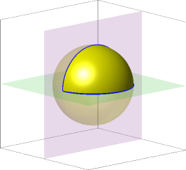
((c)) some bounded shell midsurface

\begin{overpic}[width=138.76157pt]{{Fig_3d_ImpShell4}} \put(69.0,63.0){\contour{white}{$\mathchoice{\displaystyle\bm{n}}{\textstyle\bm{n}}{\scriptstyle\bm{n}}{\scriptscriptstyle\bm{n}}_{\Gamma}$}} \put(30.0,70.0){\contour{white}{$\mathchoice{\displaystyle\bm{n}}{\textstyle\bm{n}}{\scriptstyle\bm{n}}{\scriptscriptstyle\bm{n}}_{\Gamma}$}} \put(16.0,58.0){\contour{white}{\color[rgb]{0.46,0.,0.05}$\mathchoice{\displaystyle\bm{n}}{\textstyle\bm{n}}{\scriptstyle\bm{n}}{\scriptscriptstyle\bm{n}}_{\partial\Gamma,1}$}} \put(17.0,47.0){\contour{white}{\color[rgb]{0,0.51,0}$\mathchoice{\displaystyle\bm{t}}{\textstyle\bm{t}}{\scriptstyle\bm{t}}{\scriptscriptstyle\bm{t}}_{\partial\Gamma,1}$}} \put(30.0,32.0){\contour{white}{$\mathchoice{\displaystyle\bm{n}}{\textstyle\bm{n}}{\scriptstyle\bm{n}}{\scriptscriptstyle\bm{n}}_{\Gamma}$}} \put(43.0,22.0){\contour{white}{\color[rgb]{0.46,0.,0.05}$\mathchoice{\displaystyle\bm{n}}{\textstyle\bm{n}}{\scriptstyle\bm{n}}{\scriptscriptstyle\bm{n}}_{\partial\Gamma,2}$}} \put(50.0,33.0){\contour{white}{\color[rgb]{0,0.51,0}$\mathchoice{\displaystyle\bm{t}}{\textstyle\bm{t}}{\scriptstyle\bm{t}}{\scriptscriptstyle\bm{t}}_{\partial\Gamma,2}$}} \end{overpic}

((d)) normal vector and local triads

Fig. 3: Implicit definition of a (bounded) spherical shell: $\phi(\mathchoice{\displaystyle\bm{x}}{\textstyle\bm{x}}{\scriptstyle\bm{x}}{\scriptscriptstyle\bm{x}})=\|\mathchoice{\displaystyle\bm{x}}{\textstyle\bm{x}}{\scriptstyle\bm{x}}{\scriptscriptstyle\bm{x}}\|-r,\psi_{1}(\mathchoice{\displaystyle\bm{x}}{\textstyle\bm{x}}{\scriptstyle\bm{x}}{\scriptscriptstyle\bm{x}})=x,\psi_{2}(\mathchoice{\displaystyle\bm{x}}{\textstyle\bm{x}}{\scriptstyle\bm{x}}{\scriptscriptstyle\bm{x}})=z$. (a) The colors are different isosurfaces of $\phi$, (b) implicit shell midsurface defined by the zero-isosurface of $\phi$, (c) definition of boundaries with additional slave level-set functions $\psi_{1}$ (purple) and $\psi_{2}$ (green), (d) normal (black), co-normal (red) and tangent (green) vectors.

2.1 Tangential differential calculus (TDC)

The tangential differential calculus (TDC) provides a framework to define surface operators independently of the concrete surface definition. This is an important generalization compared to classical models based on curvilinear coordinates which rely on parametrizations, i.e., explicit geometry definitions. In the following, the employed geometrical and differential operators in the frame of the TDC are briefly introduced. For a more detailed information and derivation we refer to, e.g., [27, 52, 53, 18].

On the manifold $\Gamma$, there are two projection operators $\mathchoice{\displaystyle\mathbf{Q}}{\textstyle\mathbf{Q}}{\scriptstyle\mathbf{Q}}{\scriptscriptstyle\mathbf{Q}}(\mathchoice{\displaystyle\bm{x}}{\textstyle\bm{x}}{\scriptstyle\bm{x}}{\scriptscriptstyle\bm{x}})=\mathchoice{\displaystyle\bm{n}}{\textstyle\bm{n}}{\scriptstyle\bm{n}}{\scriptscriptstyle\bm{n}}_{\Gamma}(\mathchoice{\displaystyle\bm{x}}{\textstyle\bm{x}}{\scriptstyle\bm{x}}{\scriptscriptstyle\bm{x}})\otimes\mathchoice{\displaystyle\bm{n}}{\textstyle\bm{n}}{\scriptstyle\bm{n}}{\scriptscriptstyle\bm{n}}_{\Gamma}(\mathchoice{\displaystyle\bm{x}}{\textstyle\bm{x}}{\scriptstyle\bm{x}}{\scriptscriptstyle\bm{x}})$ and $\mathchoice{\displaystyle\mathbf{P}}{\textstyle\mathbf{P}}{\scriptstyle\mathbf{P}}{\scriptscriptstyle\mathbf{P}}(\mathchoice{\displaystyle\bm{x}}{\textstyle\bm{x}}{\scriptstyle\bm{x}}{\scriptscriptstyle\bm{x}})=\mathbb{I}-\mathchoice{\displaystyle\mathbf{Q}}{\textstyle\mathbf{Q}}{\scriptstyle\mathbf{Q}}{\scriptscriptstyle\mathbf{Q}}$, where $\mathchoice{\displaystyle\mathbf{Q}}{\textstyle\mathbf{Q}}{\scriptstyle\mathbf{Q}}{\scriptscriptstyle\mathbf{Q}}$ projects an arbitrary vector $\mathchoice{\displaystyle\bm{v}}{\textstyle\bm{v}}{\scriptstyle\bm{v}}{\scriptscriptstyle\bm{v}}(\Gamma)\in\mathbb{R}^{3}$ in normal direction of $\Gamma$ and $\mathchoice{\displaystyle\mathbf{P}}{\textstyle\mathbf{P}}{\scriptstyle\mathbf{P}}{\scriptscriptstyle\mathbf{P}}$ projects an arbitrary vector onto the tangent space $T_{P}\Gamma$ of $\Gamma$.

The tangential gradient operator $\nabla_{\Gamma}$ of a differentiable scalar-valued function $u:\Gamma\to\mathbb{R}$ on the surface is given by

$$\nabla_{\Gamma}u(\mathchoice{\displaystyle\bm{x}}{\textstyle\bm{x}}{\scriptstyle\bm{x}}{\scriptscriptstyle\bm{x}}) =\mathchoice{\displaystyle\mathbf{P}}{\textstyle\mathbf{P}}{\scriptstyle\mathbf{P}}{\scriptscriptstyle\mathbf{P}}\left(\mathchoice{\displaystyle\bm{x}}{\textstyle\bm{x}}{\scriptstyle\bm{x}}{\scriptscriptstyle\bm{x}}\right)\cdot\nabla\tilde{u}\left(\mathchoice{\displaystyle\bm{x}}{\textstyle\bm{x}}{\scriptstyle\bm{x}}{\scriptscriptstyle\bm{x}}\right)\ ,\quad\mathchoice{\displaystyle\bm{x}}{\textstyle\bm{x}}{\scriptstyle\bm{x}}{\scriptscriptstyle\bm{x}}\in\Gamma$$ (2.6)

where $\nabla$ is the standard gradient operator, and $\tilde{u}$ is an arbitrarily, but sufficiently smooth extension of $u$ in a neighborhood $\mathcal{U}$ of the manifold $\Gamma$. In the context of the Trace FEM, the function $\tilde{u}$ is naturally available because all quantities are defined in the higher-dimensional space, i.e., $\mathbb{R}^{3}$ or $\Omega^{\ast}$. Therefore, $\tilde{u}$ is scalar-valued function in $\mathbb{R}^{3}$, i.e., $\tilde{u}:\mathbb{R}^{3}\to\mathbb{R}$ and the function $u$ is defined by the restriction of $\tilde{u}$ to $\Gamma$, i.e., $u:=\tilde{u}_{\rvert_{\Gamma}}$ which means that $\tilde{u}$ is only evaluated on $\Gamma$.

Applying the tangential gradient operator $\nabla_{\Gamma}$ to each component of a vector-valued function $\mathchoice{\displaystyle\bm{u}}{\textstyle\bm{u}}{\scriptstyle\bm{u}}{\scriptscriptstyle\bm{u}}\left(\mathchoice{\displaystyle\bm{x}}{\textstyle\bm{x}}{\scriptstyle\bm{x}}{\scriptscriptstyle\bm{x}}\right):\Gamma\to\mathbb{R}^{3}$, gives the directional gradient of $\mathchoice{\displaystyle\bm{u}}{\textstyle\bm{u}}{\scriptstyle\bm{u}}{\scriptscriptstyle\bm{u}}$

$$\nabla_{\Gamma}^{\text{dir}}\mathchoice{\displaystyle\bm{u}}{\textstyle\bm{u}}{\scriptstyle\bm{u}}{\scriptscriptstyle\bm{u}}\left(\mathchoice{\displaystyle\bm{x}}{\textstyle\bm{x}}{\scriptstyle\bm{x}}{\scriptscriptstyle\bm{x}}\right) =\nabla_{\Gamma}^{\text{dir}}\begin{bmatrix}u(\mathchoice{\displaystyle\bm{x}}{\textstyle\bm{x}}{\scriptstyle\bm{x}}{\scriptscriptstyle\bm{x}})\\ v(\mathchoice{\displaystyle\bm{x}}{\textstyle\bm{x}}{\scriptstyle\bm{x}}{\scriptscriptstyle\bm{x}})\\ w(\mathchoice{\displaystyle\bm{x}}{\textstyle\bm{x}}{\scriptstyle\bm{x}}{\scriptscriptstyle\bm{x}})\end{bmatrix}=\begin{bmatrix}(\nabla_{\Gamma}u)^{\mathrm{T}}\\ (\nabla_{\Gamma}v)^{\mathrm{T}}\\ (\nabla_{\Gamma}w)^{\mathrm{T}}\end{bmatrix}=\nabla\tilde{\mathchoice{\displaystyle\bm{u}}{\textstyle\bm{u}}{\scriptstyle\bm{u}}{\scriptscriptstyle\bm{u}}}\cdot\mathchoice{\displaystyle\mathbf{P}}{\textstyle\mathbf{P}}{\scriptstyle\mathbf{P}}{\scriptscriptstyle\mathbf{P}}\ ,$$

whereas the covariant gradient is defined by the projection of the directional gradient onto the tangent space, i.e., $\nabla_{\Gamma}^{\mathrm{cov}}\mathchoice{\displaystyle\bm{u}}{\textstyle\bm{u}}{\scriptstyle\bm{u}}{\scriptscriptstyle\bm{u}}\left(\mathchoice{\displaystyle\bm{x}}{\textstyle\bm{x}}{\scriptstyle\bm{x}}{\scriptscriptstyle\bm{x}}\right)=\mathchoice{\displaystyle\mathbf{P}}{\textstyle\mathbf{P}}{\scriptstyle\mathbf{P}}{\scriptscriptstyle\mathbf{P}}\cdot\nabla_{\Gamma}^{\text{dir}}\mathchoice{\displaystyle\bm{u}}{\textstyle\bm{u}}{\scriptstyle\bm{u}}{\scriptscriptstyle\bm{u}}\left(\mathchoice{\displaystyle\bm{x}}{\textstyle\bm{x}}{\scriptstyle\bm{x}}{\scriptscriptstyle\bm{x}}\right)$. The surface gradients of second-order tensor functions are defined accordingly.

Concerning the surface divergence of vector-valued functions $\mathchoice{\displaystyle\bm{u}}{\textstyle\bm{u}}{\scriptstyle\bm{u}}{\scriptscriptstyle\bm{u}}\left(\mathchoice{\displaystyle\bm{x}}{\textstyle\bm{x}}{\scriptstyle\bm{x}}{\scriptscriptstyle\bm{x}}\right):\Gamma\to\mathbb{R}^{3}$ and tensor-valued functions $\mathchoice{\displaystyle\mathbf{A}}{\textstyle\mathbf{A}}{\scriptstyle\mathbf{A}}{\scriptscriptstyle\mathbf{A}}\left(\mathchoice{\displaystyle\bm{x}}{\textstyle\bm{x}}{\scriptstyle\bm{x}}{\scriptscriptstyle\bm{x}}\right):\Gamma\to\mathbb{R}^{3\times 3}$, there holds

$$\text{div}_{\Gamma}\mathchoice{\displaystyle\bm{u}}{\textstyle\bm{u}}{\scriptstyle\bm{u}}{\scriptscriptstyle\bm{u}}\left(\mathchoice{\displaystyle\bm{x}}{\textstyle\bm{x}}{\scriptstyle\bm{x}}{\scriptscriptstyle\bm{x}}\right) =\text{div}_{\Gamma}(u,v,w)=\mathrm{tr}\left(\nabla_{\Gamma}^{\text{dir}}\mathchoice{\displaystyle\bm{u}}{\textstyle\bm{u}}{\scriptstyle\bm{u}}{\scriptscriptstyle\bm{u}}\right)=\mathrm{tr}\left(\nabla_{\Gamma}^{\text{cov}}\mathchoice{\displaystyle\bm{u}}{\textstyle\bm{u}}{\scriptstyle\bm{u}}{\scriptscriptstyle\bm{u}}\right),$$

$$\text{div}_{\Gamma}\mathchoice{\displaystyle\mathbf{A}}{\textstyle\mathbf{A}}{\scriptstyle\mathbf{A}}{\scriptscriptstyle\mathbf{A}}\left(\mathchoice{\displaystyle\bm{x}}{\textstyle\bm{x}}{\scriptstyle\bm{x}}{\scriptscriptstyle\bm{x}}\right) =\begin{bmatrix}\text{div}_{\Gamma}(A_{11},A_{12},A_{13})\\ \text{div}_{\Gamma}(A_{21},A_{22},A_{23})\\ \text{div}_{\Gamma}(A_{31},A_{32},A_{33})\end{bmatrix}\ .$$

Lastly, the surface gradient of the normal vector $\mathchoice{\displaystyle\bm{n}}{\textstyle\bm{n}}{\scriptstyle\bm{n}}{\scriptscriptstyle\bm{n}}_{\Gamma}$ yields the Weingarten map $\mathchoice{\displaystyle\mathbf{H}}{\textstyle\mathbf{H}}{\scriptstyle\mathbf{H}}{\scriptscriptstyle\mathbf{H}}=\nabla_{\Gamma}^{\text{dir}}\mathchoice{\displaystyle\bm{n}}{\textstyle\bm{n}}{\scriptstyle\bm{n}}{\scriptscriptstyle\bm{n}}_{\Gamma}=\nabla_{\Gamma}^{\text{cov}}\mathchoice{\displaystyle\bm{n}}{\textstyle\bm{n}}{\scriptstyle\bm{n}}{\scriptscriptstyle\bm{n}}_{\Gamma}$ [16, 17, 36, 52]. The Weingarten map is a symmetric in-plane tensor and its two non-zero eigenvalues are the principal curvatures $\kappa_{1,2}=-\text{eig}(\mathchoice{\displaystyle\mathbf{H}}{\textstyle\mathbf{H}}{\scriptstyle\mathbf{H}}{\scriptscriptstyle\mathbf{H}})$.

3 Governing equations

3.1 Reissner–Mindlin shells

The shell is implicitly defined by means of level-set functions. Therefore, it is a crucial requirement that the shell theory extends to this situation and the obtained boundary value problem is well-defined also on implicitly defined geometries, where a parametrization of the midsurface does not exist. Herein, the linear Reissner–Mindlin shell theory formulated in the frame of the TDC, as presented in [52, 54], is employed . The main advantage is that the used surface operators are independent of the concrete surface definition. Therefore, the usage of this shell theory in the frame of the TDC is an appealing choice. In the following, the shell equations from [52] are briefly recalled.

In [52], the displacement field $\mathchoice{\displaystyle\bm{u}}{\textstyle\bm{u}}{\scriptstyle\bm{u}}{\scriptscriptstyle\bm{u}}_{\Omega}(\mathchoice{\displaystyle\bm{x}}{\textstyle\bm{x}}{\scriptstyle\bm{x}}{\scriptscriptstyle\bm{x}})$ is decomposed into the displacement of the midsurface $\mathchoice{\displaystyle\bm{u}}{\textstyle\bm{u}}{\scriptstyle\bm{u}}{\scriptscriptstyle\bm{u}}$ and the rotation of the normal vector is modelled with a difference vector approach $\mathchoice{\displaystyle\bm{w}}{\textstyle\bm{w}}{\scriptstyle\bm{w}}{\scriptscriptstyle\bm{w}}$, see Fig. 4. The total rotation of the normal vector is split into two parts: (1) due to bending of the midsurface, (2) and due to transverse shear deformations $\mathchoice{\displaystyle\bm{\gamma}}{\textstyle\bm{\gamma}}{\scriptstyle\bm{\gamma}}{\scriptscriptstyle\bm{\gamma}}$. The coordinate in thickness direction is labelled $\zeta$ and provided that the master level-set function is a signed-distance function, $\zeta=\phi(\mathchoice{\displaystyle\bm{x}}{\textstyle\bm{x}}{\scriptstyle\bm{x}}{\scriptscriptstyle\bm{x}})$. Note that the difference vector is a tangential vector.

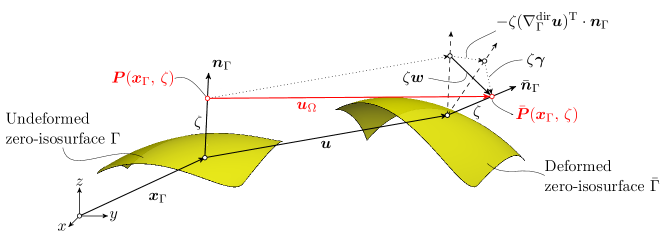
Fig. 4: Displacement field $\mathchoice{\displaystyle\bm{u}}{\textstyle\bm{u}}{\scriptstyle\bm{u}}{\scriptscriptstyle\bm{u}}_{\Omega}$ of the Reissner-Mindlin shell.

Based on the displacement field $\mathchoice{\displaystyle\bm{u}}{\textstyle\bm{u}}{\scriptstyle\bm{u}}{\scriptscriptstyle\bm{u}}_{\Omega}$, one may obtain the strain tensor $\bm{\varepsilon}_{\Gamma}$ by computing the symmetric part of the surface gradient $\nabla_{\Gamma}^{\text{dir}}\mathchoice{\displaystyle\bm{u}}{\textstyle\bm{u}}{\scriptstyle\bm{u}}{\scriptscriptstyle\bm{u}}_{\Omega}$. The strain tensor $\bm{\varepsilon}_{\Gamma}$ is split into in-plane strains $\bm{\varepsilon}_{\Gamma}^{\text{P}}$ and transverse shear strains $\bm{\varepsilon}_{\Gamma}^{\text{S}}$ using the projectors from Section 2.1

$$\bm{\varepsilon}_{\Gamma}(\mathchoice{\displaystyle\bm{x}}{\textstyle\bm{x}}{\scriptstyle\bm{x}}{\scriptscriptstyle\bm{x}}) =\bm{\varepsilon}_{\Gamma}^{\text{P}}(\mathchoice{\displaystyle\bm{x}}{\textstyle\bm{x}}{\scriptstyle\bm{x}}{\scriptscriptstyle\bm{x}})+\bm{\varepsilon}_{\Gamma}^{\text{S}}(\mathchoice{\displaystyle\bm{x}}{\textstyle\bm{x}}{\scriptstyle\bm{x}}{\scriptscriptstyle\bm{x}})\ ,$$ (3.1)

with

$$\bm{\varepsilon}_{\Gamma}^{\text{P}}(\mathchoice{\displaystyle\bm{x}}{\textstyle\bm{x}}{\scriptstyle\bm{x}}{\scriptscriptstyle\bm{x}}) =\mathchoice{\displaystyle\mathbf{P}}{\textstyle\mathbf{P}}{\scriptstyle\mathbf{P}}{\scriptscriptstyle\mathbf{P}}\cdot\bm{\varepsilon}_{\Gamma}\cdot\mathchoice{\displaystyle\mathbf{P}}{\textstyle\mathbf{P}}{\scriptstyle\mathbf{P}}{\scriptscriptstyle\mathbf{P}}=\bm{\varepsilon}_{\Gamma,\,\text{Mem}}^{\text{P}}+\zeta\,\bm{\varepsilon}_{\Gamma,\,\text{Bend}}^{\text{P}}\ ,$$ (3.2)

$$\bm{\varepsilon}_{\Gamma}^{\text{S}}(\mathchoice{\displaystyle\bm{x}}{\textstyle\bm{x}}{\scriptstyle\bm{x}}{\scriptscriptstyle\bm{x}}) =\mathchoice{\displaystyle\mathbf{Q}}{\textstyle\mathbf{Q}}{\scriptstyle\mathbf{Q}}{\scriptscriptstyle\mathbf{Q}}\cdot\bm{\varepsilon}_{\Gamma}+\bm{\varepsilon}_{\Gamma}\cdot\mathchoice{\displaystyle\mathbf{Q}}{\textstyle\mathbf{Q}}{\scriptstyle\mathbf{Q}}{\scriptscriptstyle\mathbf{Q}}\ .$$ (3.3)

The in-plane strains are further decomposed into membrane strains $\bm{\varepsilon}_{\Gamma,\,\text{Mem}}^{\text{P}}$ and bending strains $\bm{\varepsilon}_{\Gamma,\,\text{Bend}}^{\text{P}}$. In detail, the strain components are

$$\bm{\varepsilon}_{\Gamma,\,\text{Mem}}^{\text{P}}(\mathchoice{\displaystyle\bm{u}}{\textstyle\bm{u}}{\scriptstyle\bm{u}}{\scriptscriptstyle\bm{u}}) =\dfrac{1}{2}\left[\nabla_{\Gamma}^{\text{cov}}\mathchoice{\displaystyle\bm{u}}{\textstyle\bm{u}}{\scriptstyle\bm{u}}{\scriptscriptstyle\bm{u}}+(\nabla_{\Gamma}^{\text{cov}}\mathchoice{\displaystyle\bm{u}}{\textstyle\bm{u}}{\scriptstyle\bm{u}}{\scriptscriptstyle\bm{u}})^{\mathrm{T}}\right]\ ,$$ (3.4)

$$\bm{\varepsilon}_{\Gamma,\,\text{Bend}}^{\text{P}}(\mathchoice{\displaystyle\bm{u}}{\textstyle\bm{u}}{\scriptstyle\bm{u}}{\scriptscriptstyle\bm{u}},\mathchoice{\displaystyle\bm{w}}{\textstyle\bm{w}}{\scriptstyle\bm{w}}{\scriptscriptstyle\bm{w}}) =\dfrac{1}{2}\left[\mathchoice{\displaystyle\mathbf{H}}{\textstyle\mathbf{H}}{\scriptstyle\mathbf{H}}{\scriptscriptstyle\mathbf{H}}\cdot\nabla_{\Gamma}^{\text{dir}}\mathchoice{\displaystyle\bm{u}}{\textstyle\bm{u}}{\scriptstyle\bm{u}}{\scriptscriptstyle\bm{u}}+(\nabla_{\Gamma}^{\text{dir}}\mathchoice{\displaystyle\bm{u}}{\textstyle\bm{u}}{\scriptstyle\bm{u}}{\scriptscriptstyle\bm{u}})^{\mathrm{T}}\cdot\mathchoice{\displaystyle\mathbf{H}}{\textstyle\mathbf{H}}{\scriptstyle\mathbf{H}}{\scriptscriptstyle\mathbf{H}}+\nabla_{\Gamma}^{\text{cov}}\mathchoice{\displaystyle\bm{w}}{\textstyle\bm{w}}{\scriptstyle\bm{w}}{\scriptscriptstyle\bm{w}}+(\nabla_{\Gamma}^{\text{cov}}\mathchoice{\displaystyle\bm{w}}{\textstyle\bm{w}}{\scriptstyle\bm{w}}{\scriptscriptstyle\bm{w}})^{\mathrm{T}}\right]\ ,$$ (3.5)

$$\bm{\varepsilon}_{\Gamma}^{\text{S}}(\mathchoice{\displaystyle\bm{u}}{\textstyle\bm{u}}{\scriptstyle\bm{u}}{\scriptscriptstyle\bm{u}},\,\mathchoice{\displaystyle\bm{w}}{\textstyle\bm{w}}{\scriptstyle\bm{w}}{\scriptscriptstyle\bm{w}}) =\dfrac{1}{2}\left[\mathchoice{\displaystyle\mathbf{Q}}{\textstyle\mathbf{Q}}{\scriptstyle\mathbf{Q}}{\scriptscriptstyle\mathbf{Q}}\cdot\nabla_{\Gamma}^{\text{dir}}\mathchoice{\displaystyle\bm{u}}{\textstyle\bm{u}}{\scriptstyle\bm{u}}{\scriptscriptstyle\bm{u}}+(\nabla_{\Gamma}^{\text{dir}}\mathchoice{\displaystyle\bm{u}}{\textstyle\bm{u}}{\scriptstyle\bm{u}}{\scriptscriptstyle\bm{u}})^{\mathrm{T}}\cdot\mathchoice{\displaystyle\mathbf{Q}}{\textstyle\mathbf{Q}}{\scriptstyle\mathbf{Q}}{\scriptscriptstyle\mathbf{Q}}+\mathchoice{\displaystyle\bm{n}}{\textstyle\bm{n}}{\scriptstyle\bm{n}}{\scriptscriptstyle\bm{n}}_{\Gamma}\otimes\mathchoice{\displaystyle\bm{w}}{\textstyle\bm{w}}{\scriptstyle\bm{w}}{\scriptscriptstyle\bm{w}}+\mathchoice{\displaystyle\bm{w}}{\textstyle\bm{w}}{\scriptstyle\bm{w}}{\scriptscriptstyle\bm{w}}\otimes\mathchoice{\displaystyle\bm{n}}{\textstyle\bm{n}}{\scriptstyle\bm{n}}{\scriptscriptstyle\bm{n}}_{\Gamma}\right]\ .$$ (3.6)

For simplicity, we shall use a linear elastic material governed by Hooke’s law with the modified Lamé constants $\mu=\frac{E}{2(1+\nu)}$, $\lambda=\frac{E\nu}{1-\nu^{2}}$ in order to eliminate the normal stress in thickness direction. Based on that, the linear stress tensor yields

$$\bm{\sigma}_{\Gamma}(\mathchoice{\displaystyle\bm{x}}{\textstyle\bm{x}}{\scriptstyle\bm{x}}{\scriptscriptstyle\bm{x}})=2\mu\bm{\varepsilon}_{\Gamma}(\mathchoice{\displaystyle\bm{x}}{\textstyle\bm{x}}{\scriptstyle\bm{x}}{\scriptscriptstyle\bm{x}})+\lambda\text{tr}[\bm{\varepsilon}_{\Gamma}(\mathchoice{\displaystyle\bm{x}}{\textstyle\bm{x}}{\scriptstyle\bm{x}}{\scriptscriptstyle\bm{x}})]\mathbb{I}\ .$$ (3.7)

A decomposition of the stress tensor in a similar manner than the strain tensor gives the membrane, bending and transverse shear stresses. With the assumption of a constant shifter in thickness direction, an analytical pre-integration w.r.t. the thickness is possible and the stress resultants, such as moment tensor $\mathchoice{\displaystyle\mathbf{m}}{\textstyle\mathbf{m}}{\scriptstyle\mathbf{m}}{\scriptscriptstyle\mathbf{m}}_{\Gamma}$, effective normal force tensor $\tilde{\mathchoice{\displaystyle\mathbf{n}}{\textstyle\mathbf{n}}{\scriptstyle\mathbf{n}}{\scriptscriptstyle\mathbf{n}}}_{\Gamma}$ and transverse shear force tensor $\mathchoice{\displaystyle\mathbf{q}}{\textstyle\mathbf{q}}{\scriptstyle\mathbf{q}}{\scriptscriptstyle\mathbf{q}}_{\Gamma}$ are identified as

$$\begin{split}\mathchoice{\displaystyle\mathbf{m}}{\textstyle\mathbf{m}}{\scriptstyle\mathbf{m}}{\scriptscriptstyle\mathbf{m}}_{\Gamma}&=\int_{-\nicefrac{{t}}{{2}}}^{\nicefrac{{t}}{{2}}}\zeta\,\mathchoice{\displaystyle\mathbf{P}}{\textstyle\mathbf{P}}{\scriptstyle\mathbf{P}}{\scriptscriptstyle\mathbf{P}}\cdot\bm{\sigma}_{\Gamma}\cdot\mathchoice{\displaystyle\mathbf{P}}{\textstyle\mathbf{P}}{\scriptstyle\mathbf{P}}{\scriptscriptstyle\mathbf{P}}\ \mathrm{d}\zeta=\dfrac{t^{3}}{12}\bm{\sigma}_{\Gamma}^{\text{P}}(\bm{\varepsilon}^{\text{P}}_{\Gamma,\text{Bend}})\ ,\\ \tilde{\mathchoice{\displaystyle\mathbf{n}}{\textstyle\mathbf{n}}{\scriptstyle\mathbf{n}}{\scriptscriptstyle\mathbf{n}}}_{\Gamma}&=\int_{-\nicefrac{{t}}{{2}}}^{\nicefrac{{t}}{{2}}}\mathchoice{\displaystyle\mathbf{P}}{\textstyle\mathbf{P}}{\scriptstyle\mathbf{P}}{\scriptscriptstyle\mathbf{P}}\cdot\bm{\sigma}_{\Gamma}\cdot\mathchoice{\displaystyle\mathbf{P}}{\textstyle\mathbf{P}}{\scriptstyle\mathbf{P}}{\scriptscriptstyle\mathbf{P}}\ \mathrm{d}\zeta=t\bm{\sigma}_{\Gamma}^{\text{P}}(\bm{\varepsilon}^{\text{P}}_{\Gamma,\text{Mem}})\ ,\\ \mathchoice{\displaystyle\mathbf{q}}{\textstyle\mathbf{q}}{\scriptstyle\mathbf{q}}{\scriptscriptstyle\mathbf{q}}_{\Gamma}&=\int_{-\nicefrac{{t}}{{2}}}^{\nicefrac{{t}}{{2}}}\mathchoice{\displaystyle\mathbf{Q}}{\textstyle\mathbf{Q}}{\scriptstyle\mathbf{Q}}{\scriptscriptstyle\mathbf{Q}}\cdot\bm{\sigma}_{\Gamma}+\bm{\sigma}_{\Gamma}\cdot\mathchoice{\displaystyle\mathbf{Q}}{\textstyle\mathbf{Q}}{\scriptstyle\mathbf{Q}}{\scriptscriptstyle\mathbf{Q}}\ \mathrm{d}\zeta=t\bm{\sigma}_{\Gamma}^{\text{S}}(\bm{\varepsilon}^{\text{S}}_{\Gamma})\ .\end{split}$$ (3.8)

The moment and effective normal force tensors are symmetric, in-plane tensors and their two non-zero eigenvalues are the principal moments or forces, respectively. Note that in the case of curved shells, the physical normal force tensor is $\mathchoice{\displaystyle\mathbf{n}}{\textstyle\mathbf{n}}{\scriptstyle\mathbf{n}}{\scriptscriptstyle\mathbf{n}}^{\text{real}}_{\Gamma}=\tilde{\mathchoice{\displaystyle\mathbf{n}}{\textstyle\mathbf{n}}{\scriptstyle\mathbf{n}}{\scriptscriptstyle\mathbf{n}}}_{\Gamma}+\mathchoice{\displaystyle\mathbf{H}}{\textstyle\mathbf{H}}{\scriptstyle\mathbf{H}}{\scriptscriptstyle\mathbf{H}}\cdot\mathchoice{\displaystyle\mathbf{m}}{\textstyle\mathbf{m}}{\scriptstyle\mathbf{m}}{\scriptscriptstyle\mathbf{m}}_{\Gamma}$ and is, in general, not symmetric, but features one zero eigenvalue just as $\tilde{\mathchoice{\displaystyle\mathbf{n}}{\textstyle\mathbf{n}}{\scriptstyle\mathbf{n}}{\scriptscriptstyle\mathbf{n}}}_{\Gamma}$.

Based on the stress resultants, the force and moment equilibrium for an implicitly defined Reissner–Mindlin shell in strong form becomes

$$\text{div}_{\Gamma}\mathchoice{\displaystyle\mathbf{n}}{\textstyle\mathbf{n}}{\scriptstyle\mathbf{n}}{\scriptscriptstyle\mathbf{n}}^{\text{real}}_{\Gamma}+\mathchoice{\displaystyle\mathbf{Q}}{\textstyle\mathbf{Q}}{\scriptstyle\mathbf{Q}}{\scriptscriptstyle\mathbf{Q}}\cdot\text{div}_{\Gamma}\mathchoice{\displaystyle\mathbf{q}}{\textstyle\mathbf{q}}{\scriptstyle\mathbf{q}}{\scriptscriptstyle\mathbf{q}}_{\Gamma}+\mathchoice{\displaystyle\mathbf{H}}{\textstyle\mathbf{H}}{\scriptstyle\mathbf{H}}{\scriptscriptstyle\mathbf{H}}\cdot(\mathchoice{\displaystyle\mathbf{q}}{\textstyle\mathbf{q}}{\scriptstyle\mathbf{q}}{\scriptscriptstyle\mathbf{q}}_{\Gamma}\cdot\mathchoice{\displaystyle\bm{n}}{\textstyle\bm{n}}{\scriptstyle\bm{n}}{\scriptscriptstyle\bm{n}}_{\Gamma}) =-\mathchoice{\displaystyle\bm{f}}{\textstyle\bm{f}}{\scriptstyle\bm{f}}{\scriptscriptstyle\bm{f}}\ ,$$ (3.9)

$$\mathchoice{\displaystyle\mathbf{P}}{\textstyle\mathbf{P}}{\scriptstyle\mathbf{P}}{\scriptscriptstyle\mathbf{P}}\cdot\text{div}_{\Gamma}\mathchoice{\displaystyle\mathbf{m}}{\textstyle\mathbf{m}}{\scriptstyle\mathbf{m}}{\scriptscriptstyle\mathbf{m}}_{\Gamma}-\mathchoice{\displaystyle\mathbf{q}}{\textstyle\mathbf{q}}{\scriptstyle\mathbf{q}}{\scriptscriptstyle\mathbf{q}}_{\Gamma}\cdot\mathchoice{\displaystyle\bm{n}}{\textstyle\bm{n}}{\scriptstyle\bm{n}}{\scriptscriptstyle\bm{n}}_{\Gamma} =-\mathchoice{\displaystyle\bm{c}}{\textstyle\bm{c}}{\scriptstyle\bm{c}}{\scriptscriptstyle\bm{c}}\ ,$$ (3.10)

where $\mathchoice{\displaystyle\bm{f}}{\textstyle\bm{f}}{\scriptstyle\bm{f}}{\scriptscriptstyle\bm{f}}\in\mathbb{R}^{3}$ is the load vector per area and $\mathchoice{\displaystyle\bm{c}}{\textstyle\bm{c}}{\scriptstyle\bm{c}}{\scriptscriptstyle\bm{c}}\in T_{P}\Gamma$ is a distributed moment vector on the zero-isosurface $\Gamma$. The equilibriums in strong form are a set of second-order surface PDEs and with suitable boundary conditions, the complete boundary value problem (BVP) of an implicitly defined shell is defined.

For each field $\mathchoice{\displaystyle\bm{u}}{\textstyle\bm{u}}{\scriptstyle\bm{u}}{\scriptscriptstyle\bm{u}}$ and $\mathchoice{\displaystyle\bm{w}}{\textstyle\bm{w}}{\scriptstyle\bm{w}}{\scriptscriptstyle\bm{w}}$ there exist two non-overlapping parts at the boundary of the shell $\partial\Gamma$. In particular, the Dirichlet boundary $\partial\Gamma_{\text{D,i}}$ and the Neumann boundary $\partial\Gamma_{\text{N,i}}$, with $i=\{\mathchoice{\displaystyle\bm{u}}{\textstyle\bm{u}}{\scriptstyle\bm{u}}{\scriptscriptstyle\bm{u}},\,\mathchoice{\displaystyle\bm{w}}{\textstyle\bm{w}}{\scriptstyle\bm{w}}{\scriptscriptstyle\bm{w}}\}$. The corresponding boundary conditions are

$$\begin{aligned} \mathchoice{\displaystyle\bm{u}}{\textstyle\bm{u}}{\scriptstyle\bm{u}}{\scriptscriptstyle\bm{u}}&=\hat{\mathchoice{\displaystyle\bm{g}}{\textstyle\bm{g}}{\scriptstyle\bm{g}}{\scriptscriptstyle\bm{g}}}_{\mathchoice{\displaystyle\bm{u}}{\textstyle\bm{u}}{\scriptstyle\bm{u}}{\scriptscriptstyle\bm{u}}}&&\text{ on }\partial\Gamma_{\text{D},\mathchoice{\displaystyle\bm{u}}{\textstyle\bm{u}}{\scriptstyle\bm{u}}{\scriptscriptstyle\bm{u}}}\ ,\\ \mathchoice{\displaystyle\mathbf{n}}{\textstyle\mathbf{n}}{\scriptstyle\mathbf{n}}{\scriptscriptstyle\mathbf{n}}^{\text{real}}_{\Gamma}\cdot\mathchoice{\displaystyle\bm{n}}{\textstyle\bm{n}}{\scriptstyle\bm{n}}{\scriptscriptstyle\bm{n}}_{\partial\Gamma}+(\mathchoice{\displaystyle\bm{n}}{\textstyle\bm{n}}{\scriptstyle\bm{n}}{\scriptscriptstyle\bm{n}}_{\Gamma}\cdot\mathchoice{\displaystyle\mathbf{q}}{\textstyle\mathbf{q}}{\scriptstyle\mathbf{q}}{\scriptscriptstyle\mathbf{q}}_{\Gamma}\cdot\mathchoice{\displaystyle\bm{n}}{\textstyle\bm{n}}{\scriptstyle\bm{n}}{\scriptscriptstyle\bm{n}}_{\partial\Gamma})\cdot\mathchoice{\displaystyle\bm{n}}{\textstyle\bm{n}}{\scriptstyle\bm{n}}{\scriptscriptstyle\bm{n}}_{\Gamma}&=\hat{\mathchoice{\displaystyle\bm{p}}{\textstyle\bm{p}}{\scriptstyle\bm{p}}{\scriptscriptstyle\bm{p}}}&&\text{ on }\partial\Gamma_{\text{N},\mathchoice{\displaystyle\bm{u}}{\textstyle\bm{u}}{\scriptstyle\bm{u}}{\scriptscriptstyle\bm{u}}}\ ,\\ \mathchoice{\displaystyle\bm{w}}{\textstyle\bm{w}}{\scriptstyle\bm{w}}{\scriptscriptstyle\bm{w}}&=\hat{\mathchoice{\displaystyle\bm{g}}{\textstyle\bm{g}}{\scriptstyle\bm{g}}{\scriptscriptstyle\bm{g}}}_{\mathchoice{\displaystyle\bm{w}}{\textstyle\bm{w}}{\scriptstyle\bm{w}}{\scriptscriptstyle\bm{w}}}&&\text{ on }\partial\Gamma_{\text{D},\mathchoice{\displaystyle\bm{w}}{\textstyle\bm{w}}{\scriptstyle\bm{w}}{\scriptscriptstyle\bm{w}}}\ ,\\ \mathchoice{\displaystyle\mathbf{m}}{\textstyle\mathbf{m}}{\scriptstyle\mathbf{m}}{\scriptscriptstyle\mathbf{m}}_{\Gamma}\cdot\mathchoice{\displaystyle\bm{n}}{\textstyle\bm{n}}{\scriptstyle\bm{n}}{\scriptscriptstyle\bm{n}}_{\partial\Gamma}&=\hat{\mathchoice{\displaystyle\bm{m}}{\textstyle\bm{m}}{\scriptstyle\bm{m}}{\scriptscriptstyle\bm{m}}}_{\partial\Gamma}&&\text{ on }\partial\Gamma_{\text{N},\mathchoice{\displaystyle\bm{w}}{\textstyle\bm{w}}{\scriptstyle\bm{w}}{\scriptscriptstyle\bm{w}}}\ ,\end{aligned}$$ (3.11)

where $\hat{\mathchoice{\displaystyle\bm{g}}{\textstyle\bm{g}}{\scriptstyle\bm{g}}{\scriptscriptstyle\bm{g}}}_{\mathchoice{\displaystyle\bm{u}}{\textstyle\bm{u}}{\scriptstyle\bm{u}}{\scriptscriptstyle\bm{u}}}$ are the displacements, $\hat{\mathchoice{\displaystyle\bm{g}}{\textstyle\bm{g}}{\scriptstyle\bm{g}}{\scriptscriptstyle\bm{g}}}_{\mathchoice{\displaystyle\bm{w}}{\textstyle\bm{w}}{\scriptstyle\bm{w}}{\scriptscriptstyle\bm{w}}}$ are the rotations of the normal vector, $\hat{\mathchoice{\displaystyle\bm{p}}{\textstyle\bm{p}}{\scriptstyle\bm{p}}{\scriptscriptstyle\bm{p}}}$ are the forces and $\hat{\mathchoice{\displaystyle\bm{m}}{\textstyle\bm{m}}{\scriptstyle\bm{m}}{\scriptscriptstyle\bm{m}}}_{\partial\Gamma}$ are the bending moments at their corresponding part of the boundary. For a more detailed discussion regarding the natural and essential boundary conditions, we refer to [52].

3.2 Equilibrium in weak form

In order to convert the equilibrium in strong form to the weak form, we introduce the following function spaces

$$\mathcal{S}_{\mathchoice{\displaystyle\bm{u}}{\textstyle\bm{u}}{\scriptstyle\bm{u}}{\scriptscriptstyle\bm{u}}} =\left\{\mathchoice{\displaystyle\bm{v}}{\textstyle\bm{v}}{\scriptstyle\bm{v}}{\scriptscriptstyle\bm{v}}\in\left[\mathcal{H}^{1}(\Gamma)\right]^{3}:\mathchoice{\displaystyle\bm{v}}{\textstyle\bm{v}}{\scriptstyle\bm{v}}{\scriptscriptstyle\bm{v}}=\hat{\mathchoice{\displaystyle\bm{g}}{\textstyle\bm{g}}{\scriptstyle\bm{g}}{\scriptscriptstyle\bm{g}}}_{\mathchoice{\displaystyle\bm{u}}{\textstyle\bm{u}}{\scriptstyle\bm{u}}{\scriptscriptstyle\bm{u}}}\text{ on }\partial\Gamma_{\text{D},\mathchoice{\displaystyle\bm{u}}{\textstyle\bm{u}}{\scriptstyle\bm{u}}{\scriptscriptstyle\bm{u}}}\right\}\ ,$$ (3.12)

$$\mathcal{V}_{\mathchoice{\displaystyle\bm{u}}{\textstyle\bm{u}}{\scriptstyle\bm{u}}{\scriptscriptstyle\bm{u}}} =\left\{\mathchoice{\displaystyle\bm{v}}{\textstyle\bm{v}}{\scriptstyle\bm{v}}{\scriptscriptstyle\bm{v}}\in\left[\mathcal{H}^{1}(\Gamma)\right]^{3}:\mathchoice{\displaystyle\bm{v}}{\textstyle\bm{v}}{\scriptstyle\bm{v}}{\scriptscriptstyle\bm{v}}=\mathchoice{\displaystyle\bm{0}}{\textstyle\bm{0}}{\scriptstyle\bm{0}}{\scriptscriptstyle\bm{0}}\text{ on }\partial\Gamma_{\text{D},\mathchoice{\displaystyle\bm{u}}{\textstyle\bm{u}}{\scriptstyle\bm{u}}{\scriptscriptstyle\bm{u}}}\right\}\ ,$$ (3.13)

$$\mathcal{S}_{\mathchoice{\displaystyle\bm{w}}{\textstyle\bm{w}}{\scriptstyle\bm{w}}{\scriptscriptstyle\bm{w}}} =\left\{\mathchoice{\displaystyle\bm{v}}{\textstyle\bm{v}}{\scriptstyle\bm{v}}{\scriptscriptstyle\bm{v}}\in\left[\mathcal{H}^{1}(\Gamma)\right]^{3}:\mathchoice{\displaystyle\bm{v}}{\textstyle\bm{v}}{\scriptstyle\bm{v}}{\scriptscriptstyle\bm{v}}\cdot\mathchoice{\displaystyle\bm{n}}{\textstyle\bm{n}}{\scriptstyle\bm{n}}{\scriptscriptstyle\bm{n}}_{\Gamma}=0\ ;\ \mathchoice{\displaystyle\bm{v}}{\textstyle\bm{v}}{\scriptstyle\bm{v}}{\scriptscriptstyle\bm{v}}=\hat{\mathchoice{\displaystyle\bm{g}}{\textstyle\bm{g}}{\scriptstyle\bm{g}}{\scriptscriptstyle\bm{g}}}_{\mathchoice{\displaystyle\bm{w}}{\textstyle\bm{w}}{\scriptstyle\bm{w}}{\scriptscriptstyle\bm{w}}}\text{ on }\partial\Gamma_{\text{D},\mathchoice{\displaystyle\bm{w}}{\textstyle\bm{w}}{\scriptstyle\bm{w}}{\scriptscriptstyle\bm{w}}}\right\}\ ,$$ (3.14)

$$\mathcal{V}_{\mathchoice{\displaystyle\bm{w}}{\textstyle\bm{w}}{\scriptstyle\bm{w}}{\scriptscriptstyle\bm{w}}} =\left\{\mathchoice{\displaystyle\bm{v}}{\textstyle\bm{v}}{\scriptstyle\bm{v}}{\scriptscriptstyle\bm{v}}\in\left[\mathcal{H}^{1}(\Gamma)\right]^{3}:\mathchoice{\displaystyle\bm{v}}{\textstyle\bm{v}}{\scriptstyle\bm{v}}{\scriptscriptstyle\bm{v}}\cdot\mathchoice{\displaystyle\bm{n}}{\textstyle\bm{n}}{\scriptstyle\bm{n}}{\scriptscriptstyle\bm{n}}_{\Gamma}=0\ ;\ \mathchoice{\displaystyle\bm{v}}{\textstyle\bm{v}}{\scriptstyle\bm{v}}{\scriptscriptstyle\bm{v}}=0\text{ on }\partial\Gamma_{\text{D},\mathchoice{\displaystyle\bm{w}}{\textstyle\bm{w}}{\scriptstyle\bm{w}}{\scriptscriptstyle\bm{w}}}\right\}\ ,$$ (3.15)

where $\mathcal{H}^{1}$ is the space of functions with square integrable first derivatives. Note that the functions are 3D functions on the midsurface, i.e, $\mathchoice{\displaystyle\bm{v}}{\textstyle\bm{v}}{\scriptstyle\bm{v}}{\scriptscriptstyle\bm{v}}(\mathchoice{\displaystyle\bm{x}}{\textstyle\bm{x}}{\scriptstyle\bm{x}}{\scriptscriptstyle\bm{x}}):\Gamma\to\mathbb{R}^{3},\mathchoice{\displaystyle\bm{x}}{\textstyle\bm{x}}{\scriptstyle\bm{x}}{\scriptscriptstyle\bm{x}}\in\Gamma\subset\mathbb{R}^{3}$. The non-tangential spaces $(\mathcal{S}_{\mathchoice{\displaystyle\bm{u}}{\textstyle\bm{u}}{\scriptstyle\bm{u}}{\scriptscriptstyle\bm{u}}},\mathcal{V}_{\mathchoice{\displaystyle\bm{u}}{\textstyle\bm{u}}{\scriptstyle\bm{u}}{\scriptscriptstyle\bm{u}}})$ are employed for the trial and test functions of the midsurface displacement, whereas the tangential function spaces $(\mathcal{S}_{\mathchoice{\displaystyle\bm{w}}{\textstyle\bm{w}}{\scriptstyle\bm{w}}{\scriptscriptstyle\bm{w}}},\mathcal{V}_{\mathchoice{\displaystyle\bm{w}}{\textstyle\bm{w}}{\scriptstyle\bm{w}}{\scriptscriptstyle\bm{w}}})$ are used for the trial and test functions of the difference vector, which need to be tangential according to the Reissner–Mindlin kinematics. Later on for the discrete problem in the frame of the Trace FEM, these functions are defined in the physical space $\mathbb{R}^{3}$ and then restricted to $\Gamma$, with the additional condition that the functions need to be in $[\mathcal{H}^{1}(\Gamma)]^{3}$. It is emphasized that the definition of the functions in the higher-dimensional space and then restricting them to the trace (midsurface) is one of the major differences compared to classical Surface FEM.

With the above defined function spaces, see Eq. 3.12 - Eq. 3.15, the weak form of the equilibrium reads as follows: Given material parameters $(E,\nu)\in\mathbb{R}^{+}$, body forces $\mathchoice{\displaystyle\bm{f}}{\textstyle\bm{f}}{\scriptstyle\bm{f}}{\scriptscriptstyle\bm{f}}\in\mathbb{R}^{3}$ on $\Gamma$, tractions $\hat{\mathchoice{\displaystyle\bm{p}}{\textstyle\bm{p}}{\scriptstyle\bm{p}}{\scriptscriptstyle\bm{p}}}$ on $\partial\Gamma_{\text{N},\mathchoice{\displaystyle\bm{u}}{\textstyle\bm{u}}{\scriptstyle\bm{u}}{\scriptscriptstyle\bm{u}}}$, find $\mathchoice{\displaystyle\bm{u}}{\textstyle\bm{u}}{\scriptstyle\bm{u}}{\scriptscriptstyle\bm{u}}\in\mathcal{S}_{\mathchoice{\displaystyle\bm{u}}{\textstyle\bm{u}}{\scriptstyle\bm{u}}{\scriptscriptstyle\bm{u}}}$ and $\mathchoice{\displaystyle\bm{w}}{\textstyle\bm{w}}{\scriptstyle\bm{w}}{\scriptscriptstyle\bm{w}}\in\mathcal{S}_{\mathchoice{\displaystyle\bm{w}}{\textstyle\bm{w}}{\scriptstyle\bm{w}}{\scriptscriptstyle\bm{w}}}$ such that for all $\mathchoice{\displaystyle\bm{v}}{\textstyle\bm{v}}{\scriptstyle\bm{v}}{\scriptscriptstyle\bm{v}}_{\mathchoice{\displaystyle\bm{u}}{\textstyle\bm{u}}{\scriptstyle\bm{u}}{\scriptscriptstyle\bm{u}}}\in\mathcal{V}_{\mathchoice{\displaystyle\bm{u}}{\textstyle\bm{u}}{\scriptstyle\bm{u}}{\scriptscriptstyle\bm{u}}}$, there holds

$$\begin{split}\int_{\Gamma}\nabla_{\Gamma}^{\text{dir}}\mathchoice{\displaystyle\bm{v}}{\textstyle\bm{v}}{\scriptstyle\bm{v}}{\scriptscriptstyle\bm{v}}_{u}:\tilde{\mathchoice{\displaystyle\mathbf{n}}{\textstyle\mathbf{n}}{\scriptstyle\mathbf{n}}{\scriptscriptstyle\mathbf{n}}}_{\Gamma}+(\mathchoice{\displaystyle\mathbf{H}}{\textstyle\mathbf{H}}{\scriptstyle\mathbf{H}}{\scriptscriptstyle\mathbf{H}}\cdot\nabla_{\Gamma}^{\text{dir}}\mathchoice{\displaystyle\bm{v}}{\textstyle\bm{v}}{\scriptstyle\bm{v}}{\scriptscriptstyle\bm{v}}_{u}):\mathchoice{\displaystyle\mathbf{m}}{\textstyle\mathbf{m}}{\scriptstyle\mathbf{m}}{\scriptscriptstyle\mathbf{m}}_{\Gamma}+(\mathchoice{\displaystyle\mathbf{Q}}{\textstyle\mathbf{Q}}{\scriptstyle\mathbf{Q}}{\scriptscriptstyle\mathbf{Q}}\cdot\nabla_{\Gamma}^{\text{dir}}\mathchoice{\displaystyle\bm{v}}{\textstyle\bm{v}}{\scriptstyle\bm{v}}{\scriptscriptstyle\bm{v}}_{u}):\mathchoice{\displaystyle\mathbf{q}}{\textstyle\mathbf{q}}{\scriptstyle\mathbf{q}}{\scriptscriptstyle\mathbf{q}}_{\Gamma}\ \mathrm{d}A&=\int_{\Gamma}\mathchoice{\displaystyle\bm{v}}{\textstyle\bm{v}}{\scriptstyle\bm{v}}{\scriptscriptstyle\bm{v}}_{u}\cdot\mathchoice{\displaystyle\bm{f}}{\textstyle\bm{f}}{\scriptstyle\bm{f}}{\scriptscriptstyle\bm{f}}\ \mathrm{d}A+\int_{\partial\Gamma_{\text{N},\mathchoice{\displaystyle\bm{u}}{\textstyle\bm{u}}{\scriptstyle\bm{u}}{\scriptscriptstyle\bm{u}}}}\mathchoice{\displaystyle\bm{v}}{\textstyle\bm{v}}{\scriptstyle\bm{v}}{\scriptscriptstyle\bm{v}}_{u}\cdot\hat{\mathchoice{\displaystyle\bm{p}}{\textstyle\bm{p}}{\scriptstyle\bm{p}}{\scriptscriptstyle\bm{p}}}\ \mathrm{d}s\ .\end{split}$$ (3.16)

The weak form of the moment equilibrium reads as follows: Given material parameters $(E,\nu)\in\mathbb{R}^{+}$, distributed moments $\mathchoice{\displaystyle\bm{c}}{\textstyle\bm{c}}{\scriptstyle\bm{c}}{\scriptscriptstyle\bm{c}}\in T_{P}\Gamma$ on $\Gamma$, bending moments $\hat{\mathchoice{\displaystyle\bm{m}}{\textstyle\bm{m}}{\scriptstyle\bm{m}}{\scriptscriptstyle\bm{m}}}_{\partial\Gamma}$ on $\partial\Gamma_{\text{N},\mathchoice{\displaystyle\bm{w}}{\textstyle\bm{w}}{\scriptstyle\bm{w}}{\scriptscriptstyle\bm{w}}}$, find $\mathchoice{\displaystyle\bm{u}}{\textstyle\bm{u}}{\scriptstyle\bm{u}}{\scriptscriptstyle\bm{u}}\in\mathcal{S}_{\mathchoice{\displaystyle\bm{u}}{\textstyle\bm{u}}{\scriptstyle\bm{u}}{\scriptscriptstyle\bm{u}}}$ and $\mathchoice{\displaystyle\bm{w}}{\textstyle\bm{w}}{\scriptstyle\bm{w}}{\scriptscriptstyle\bm{w}}\in\mathcal{V}_{\mathchoice{\displaystyle\bm{w}}{\textstyle\bm{w}}{\scriptstyle\bm{w}}{\scriptscriptstyle\bm{w}}}$ such that for all $\mathchoice{\displaystyle\bm{v}}{\textstyle\bm{v}}{\scriptstyle\bm{v}}{\scriptscriptstyle\bm{v}}_{\mathchoice{\displaystyle\bm{w}}{\textstyle\bm{w}}{\scriptstyle\bm{w}}{\scriptscriptstyle\bm{w}}}\in\mathcal{V}_{\mathchoice{\displaystyle\bm{w}}{\textstyle\bm{w}}{\scriptstyle\bm{w}}{\scriptscriptstyle\bm{w}}}$, there holds

$$\begin{split}\int_{\Gamma}\nabla_{\Gamma}^{\text{dir}}\mathchoice{\displaystyle\bm{v}}{\textstyle\bm{v}}{\scriptstyle\bm{v}}{\scriptscriptstyle\bm{v}}_{w}:\mathchoice{\displaystyle\mathbf{m}}{\textstyle\mathbf{m}}{\scriptstyle\mathbf{m}}{\scriptscriptstyle\mathbf{m}}_{\Gamma}+\mathchoice{\displaystyle\bm{v}}{\textstyle\bm{v}}{\scriptstyle\bm{v}}{\scriptscriptstyle\bm{v}}_{w}\cdot(\mathchoice{\displaystyle\mathbf{q}}{\textstyle\mathbf{q}}{\scriptstyle\mathbf{q}}{\scriptscriptstyle\mathbf{q}}_{\Gamma}\cdot\mathchoice{\displaystyle\bm{n}}{\textstyle\bm{n}}{\scriptstyle\bm{n}}{\scriptscriptstyle\bm{n}}_{\Gamma})\ \mathrm{d}A&=\int_{\Gamma}\mathchoice{\displaystyle\bm{v}}{\textstyle\bm{v}}{\scriptstyle\bm{v}}{\scriptscriptstyle\bm{v}}_{w}\cdot\mathchoice{\displaystyle\bm{c}}{\textstyle\bm{c}}{\scriptstyle\bm{c}}{\scriptscriptstyle\bm{c}}\ \mathrm{d}A+\int_{\partial\Gamma_{\text{N},\mathchoice{\displaystyle\bm{w}}{\textstyle\bm{w}}{\scriptstyle\bm{w}}{\scriptscriptstyle\bm{w}}}}\mathchoice{\displaystyle\bm{v}}{\textstyle\bm{v}}{\scriptstyle\bm{v}}{\scriptscriptstyle\bm{v}}_{w}\cdot\hat{\mathchoice{\displaystyle\bm{m}}{\textstyle\bm{m}}{\scriptstyle\bm{m}}{\scriptscriptstyle\bm{m}}}_{\partial\Gamma}\ \mathrm{d}s\ .\end{split}$$ (3.17)

For further details regarding the derivation of the shell equations in the frame of the TDC and the used identities in order to obtain the equilibrium in weak form, we refer the interested reader to [52].

4 Trace Finite Element Method

The obtained weak form of the equilibrium is discretized with a trace finite element approach (Trace FEM), see, e.g., [46, 44, 49, 45, 31, 29, 54]. This approach is a fictitious domain method for surface PDEs, where the implicitly defined domain of interest $\Gamma$ is completely immersed in a background domain $\Omega_{\text{B}}\in\mathbb{R}^{3}$ and a parametrization of $\Gamma$ is neither available nor needed. Let us first introduce fundamental terms and quantities, which are required in order to discretize a surface PDE with the Trace FEM. The main ingredients for the Trace FEM are the definition of (1) the background mesh, (2) the discrete domain of interest $(\Gamma^{h},\partial\Gamma^{h})$, and (3) the Trace FEM function space.

Firstly, a background mesh $\Omega_{\text{B}}$, which completely immerses the domain of interest, i.e., the midsurface of the shell $\Gamma\in\Omega_{\text{B}}$, needs to be defined. Without loss of generality, the mesh can be defined by a set $\tau_{\text{B}}$ of 3D elements and is not restricted to a certain element type. Herein, the background mesh consists of tetrahedral elements $T$ of complete order $k\geq 1$. The background mesh is then defined by $\Omega_{\text{B}}:=\underset{T\in\tau_{h}}{\cup}T\in C^{0}$. Associated to the reference element $\bar{T}$, there is a fixed set of basis functions $\{N_{i}^{k}(\mathchoice{\displaystyle\bm{r}}{\textstyle\bm{r}}{\scriptstyle\bm{r}}{\scriptscriptstyle\bm{r}})\}$, with $i=1,\ldots,n_{\text{nodes}}$ being the number of nodes per element. The shape functions are Lagrange basis functions, i.e., $N_{i}^{k}(\mathchoice{\displaystyle\bm{r}_{j}}{\textstyle\bm{r}_{j}}{\scriptstyle\bm{r}_{j}}{\scriptscriptstyle\bm{r}_{j}})=\delta_{ij}$ and $N_{i}^{k}(\mathchoice{\displaystyle\bm{r}}{\textstyle\bm{r}}{\scriptstyle\bm{r}}{\scriptscriptstyle\bm{r}})\in\mathbb{P}^{k}(\bar{T})$, where $\mathbb{P}^{k}(\bar{T})$ is the polynomial basis for 3D tetrahedral Lagrange elements of complete order $k$. With an atlas of local, element-wise mappings from the 3D reference element to the 3D physical elements $\mathchoice{\displaystyle\bm{x}}{\textstyle\bm{x}}{\scriptstyle\bm{x}}{\scriptscriptstyle\bm{x}}(\mathchoice{\displaystyle\bm{r}}{\textstyle\bm{r}}{\scriptstyle\bm{r}}{\scriptscriptstyle\bm{r}}):\bar{T}\to T$, with $\mathchoice{\displaystyle\bm{x}}{\textstyle\bm{x}}{\scriptstyle\bm{x}}{\scriptscriptstyle\bm{x}}(\mathchoice{\displaystyle\bm{r}}{\textstyle\bm{r}}{\scriptstyle\bm{r}}{\scriptscriptstyle\bm{r}})=N^{k}_{i}(\mathchoice{\displaystyle\bm{r}}{\textstyle\bm{r}}{\scriptstyle\bm{r}}{\scriptscriptstyle\bm{r}})\mathchoice{\displaystyle\bm{x}}{\textstyle\bm{x}}{\scriptstyle\bm{x}}{\scriptscriptstyle\bm{x}}_{i}$, $\mathchoice{\displaystyle\bm{r}}{\textstyle\bm{r}}{\scriptstyle\bm{r}}{\scriptscriptstyle\bm{r}}\in\bar{T}$, $\mathchoice{\displaystyle\bm{x}}{\textstyle\bm{x}}{\scriptstyle\bm{x}}{\scriptscriptstyle\bm{x}}_{i}\in T$, where $\mathchoice{\displaystyle\bm{x}}{\textstyle\bm{x}}{\scriptstyle\bm{x}}{\scriptscriptstyle\bm{x}}_{i}$ are the nodal coordinates, one may define shape functions $N_{i}^{k}(\mathchoice{\displaystyle\bm{x}}{\textstyle\bm{x}}{\scriptstyle\bm{x}}{\scriptscriptstyle\bm{x}})$ be means of the isoparametric concept. The union of all elements forms a global set of $C^{0}$-continuous basis functions $\{M_{l}^{k}(\mathchoice{\displaystyle\bm{x}}{\textstyle\bm{x}}{\scriptstyle\bm{x}}{\scriptscriptstyle\bm{x}})\}$ in $\Omega_{\text{B}}$ with $l=1,\ldots,n$ and $n$ being the total number of nodes of the mesh. A general finite element space is then defined as

$$\mathcal{Q}^{k}_{\Omega_{\text{B}},h}:=\left\{v_{h}\in C^{0}(\Omega_{\text{B}})\ |\ v_{h}=\sum_{l=1}^{n}M_{l}^{k}(\mathchoice{\displaystyle\bm{x}}{\textstyle\bm{x}}{\scriptstyle\bm{x}}{\scriptscriptstyle\bm{x}})\hat{v}_{l}\ |\ \hat{v}_{l}\in\mathbb{R}\right\}\subset\mathcal{H}^{1}(\Omega_{\text{B}})\ .$$ (4.1)

Secondly, the implicitly defined geometry of the shell is defined with a set of level-set functions, see Section 2. The continuous level-set functions $(\phi,\psi_{i})$ are interpolated with the shape functions $\{M_{l}^{k}(\mathchoice{\displaystyle\bm{X}}{\textstyle\bm{X}}{\scriptstyle\bm{X}}{\scriptscriptstyle\bm{X}})\}$ of the background mesh based on their nodal values, i.e., $\hat{\phi}_{l}=\phi(\mathchoice{\displaystyle\bm{x}}{\textstyle\bm{x}}{\scriptstyle\bm{x}}{\scriptscriptstyle\bm{x}}_{l}),\hat{\psi}_{j,l}=\psi_{j}(\mathchoice{\displaystyle\bm{x}}{\textstyle\bm{x}}{\scriptstyle\bm{x}}{\scriptscriptstyle\bm{x}}_{l})$. This means that the level-set data is only needed at the nodes of the background mesh $\Omega_{\text{B}}$. The discrete shell midsurface $\Gamma^{h}$ is then implied by $\phi^{h}$ and the discrete boundaries of the shell $\partial\Gamma^{h}$ may be defined either through the discrete slave level-set functions $\psi_{i}^{h}$ or the boundary of the background mesh. In the following, the discrete boundary is only defined with additional slave level-set functions, otherwise the overall approach would be limited to a boundary conforming background mesh. The discrete normal vector $\mathchoice{\displaystyle\bm{n}}{\textstyle\bm{n}}{\scriptstyle\bm{n}}{\scriptscriptstyle\bm{n}}_{\Gamma}^{h}$ and the discrete local triad at the boundaries $(\mathchoice{\displaystyle\bm{n}}{\textstyle\bm{n}}{\scriptstyle\bm{n}}{\scriptscriptstyle\bm{n}}_{\Gamma}^{h},\mathchoice{\displaystyle\bm{n}}{\textstyle\bm{n}}{\scriptstyle\bm{n}}{\scriptscriptstyle\bm{n}}_{\partial\Gamma}^{h},\mathchoice{\displaystyle\bm{t}}{\textstyle\bm{t}}{\scriptstyle\bm{t}}{\scriptscriptstyle\bm{t}}_{\partial\Gamma}^{h})$ are evaluated on the discrete zero-isosurface of $\phi^{h}$. For the computation of the normal vector and local triads, one may employ the exact gradients of the level-set functions $(\phi,\psi_{i})$ or, alternatively, the interpolated level-set functions $(\phi^{h},\psi_{i}^{h})$. Herein, the latter approach based on the interpolated level-set data is used, resulting in

$$\mathchoice{\displaystyle\bm{n}}{\textstyle\bm{n}}{\scriptstyle\bm{n}}{\scriptscriptstyle\bm{n}}_{\Gamma}^{h}(\mathchoice{\displaystyle\bm{x}}{\textstyle\bm{x}}{\scriptstyle\bm{x}}{\scriptscriptstyle\bm{x}})=\dfrac{\nabla\phi^{h}(\mathchoice{\displaystyle\bm{x}}{\textstyle\bm{x}}{\scriptstyle\bm{x}}{\scriptscriptstyle\bm{x}})}{\|\nabla\phi^{h}(\mathchoice{\displaystyle\bm{x}}{\textstyle\bm{x}}{\scriptstyle\bm{x}}{\scriptscriptstyle\bm{x}})\|}\,, \mathchoice{\displaystyle\bm{t}}{\textstyle\bm{t}}{\scriptstyle\bm{t}}{\scriptscriptstyle\bm{t}}_{\partial\Gamma,i}^{h}(\mathchoice{\displaystyle\bm{x}}{\textstyle\bm{x}}{\scriptstyle\bm{x}}{\scriptscriptstyle\bm{x}})=\dfrac{\psi_{i}^{h}(\mathchoice{\displaystyle\bm{x}}{\textstyle\bm{x}}{\scriptstyle\bm{x}}{\scriptscriptstyle\bm{x}})\times\phi^{h}(\mathchoice{\displaystyle\bm{x}}{\textstyle\bm{x}}{\scriptstyle\bm{x}}{\scriptscriptstyle\bm{x}})}{\|\psi_{i}^{h}(\mathchoice{\displaystyle\bm{x}}{\textstyle\bm{x}}{\scriptstyle\bm{x}}{\scriptscriptstyle\bm{x}})\times\phi^{h}(\mathchoice{\displaystyle\bm{x}}{\textstyle\bm{x}}{\scriptstyle\bm{x}}{\scriptscriptstyle\bm{x}})\|}\,, \mathchoice{\displaystyle\bm{n}}{\textstyle\bm{n}}{\scriptstyle\bm{n}}{\scriptscriptstyle\bm{n}}_{\partial\Gamma,i}^{h}=\mathchoice{\displaystyle\bm{t}}{\textstyle\bm{t}}{\scriptstyle\bm{t}}{\scriptscriptstyle\bm{t}}^{h}_{\partial\Gamma,i}(\mathchoice{\displaystyle\bm{x}}{\textstyle\bm{x}}{\scriptstyle\bm{x}}{\scriptscriptstyle\bm{x}})\times\mathchoice{\displaystyle\bm{n}}{\textstyle\bm{n}}{\scriptstyle\bm{n}}{\scriptscriptstyle\bm{n}}_{\Gamma}^{h}(\mathchoice{\displaystyle\bm{x}}{\textstyle\bm{x}}{\scriptstyle\bm{x}}{\scriptscriptstyle\bm{x}})\,,$$

where $\mathchoice{\displaystyle\bm{x}}{\textstyle\bm{x}}{\scriptstyle\bm{x}}{\scriptscriptstyle\bm{x}}\in\Gamma^{h}\cup\partial\Gamma^{h}$. The projectors $\mathchoice{\displaystyle\mathbf{P}}{\textstyle\mathbf{P}}{\scriptstyle\mathbf{P}}{\scriptscriptstyle\mathbf{P}}$ and $\mathchoice{\displaystyle\mathbf{Q}}{\textstyle\mathbf{Q}}{\scriptstyle\mathbf{Q}}{\scriptscriptstyle\mathbf{Q}}$ are then computed by means of the discrete normal vector $\mathchoice{\displaystyle\bm{n}}{\textstyle\bm{n}}{\scriptstyle\bm{n}}{\scriptscriptstyle\bm{n}}_{\Gamma}^{h}$. It is clear that the gradients of $(\phi^{h},\psi_{i}^{h})$ are not exact and an additional source of error is added. However, the level-set functions are interpolated using quasi-uniform, higher-order background elements and it is shown in the numerical results in Section 5 that optimal convergence rates are achieved. Thus, the additional error caused by employing interpolated level-set data is often acceptable.

The set of elements with a non-empty intersection with $\Gamma^{h}$ is denoted by $\tau_{\Omega,h}^{\Gamma}$ and defines the active mesh $\Omega^{\Gamma}_{h}:=\underset{T\in\tau_{\Omega,h}^{\Gamma}}{\cup}T$. The definition of the active mesh is a crucial task, because the nodes of the active mesh imply the degrees of freedom in the numerical simulation.

Lastly, the Trace FEM function space $\mathcal{T}_{h}$ is established by the restriction of a “higher-dimensional finite element space” the active mesh $\Omega^{\Gamma}_{h}$. The finite element space of the active mesh $\mathcal{Q}^{k}_{\Omega^{\Gamma}_{h}}$ is defined in a similar manner as $\mathcal{Q}^{k}_{\Omega_{\text{B}},h}$, but contains only cut background elements. A general Trace FEM function space $\mathcal{T}_{h}$ is then defined by

$$\mathcal{T}_{h}=\left\{v\in\mathcal{Q}^{k}_{\Omega^{\Gamma}_{h}}\ :\ v\rvert_{\Gamma^{h}}\in\mathcal{H}^{1}(\Gamma^{h})\right\}\ \subset\mathcal{H}^{1}(\Omega_{\text{B}})\ .$$ (4.2)

4.1 Implementational aspects of the Trace FEM

As mentioned above, the Trace FEM is a fictitious domain method and, compared to standard Surface finite element approaches, three well-known challenges arise which are further outlined below: (i) integration of the weak form on the discrete zero-isosurface and its boundaries, (ii) stabilization of the stiffness matrix due to the restriction of the shape functions to the trace and small supports due to unfavourable cut scenarios and (iii) the enforcement of essential boundary conditions. In the following, these challenges are addressed in detail enabling a higher-order Trace FEM approach.

4.1.1 Higher-order accurate integration of the discrete zero-isosurface

The numerical integration of the domain of interest, i.e., on the zero-isosurface of $\phi$, is a non-trivial task, in particular with higher-order accuracy. One approach which is suitable for higher-order is presented in [40]. The numerical integration is based on a higher-order accurate lift of a linear reconstruction of the zero-isosurface. However, the extension to multiple level-set functions, where the zero-isosurface of the master level-set function is restricted with additional slave-level-set functions has not been addressed so far.

Herein, we employ the integration strategy outlined by the authors in [24, 25, 26, 27]. The advantages of this particular approach are an optimal higher-order accurate integration and a natural extension to multiple level-set functions. In this approach, the placement of the integration points on the discrete zero-isosurface is based on a higher-order, recursive reconstruction in the cut reference element. That is, the shell midsurface is reconstructed by higher-order surface elements. It is important that the reconstructed surface element is only used for the generation of integration points in the 3D reference element and may be interpreted as an integration cell. In Fig. 5, an overview of the procedure is illustrated. The yellow surface is the implicitly defined zero-isosurface of $\phi^{h}$ and is restricted by additional slave level-set functions $\psi_{i}^{h}$ (green and purple surfaces). In Fig. 5(b), the cut scenario and integration points in the reference space of the red marked element from Fig. 5(a) are visualized. In Fig. 5(c), the integration points in the physical domain (red) and on the boundaries (blue) are shown. For further information and details, we refer to [24, 25].

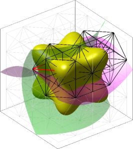
((a)) active background elements

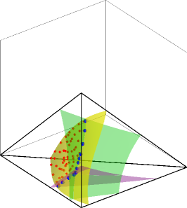
((b)) integration points in reference element

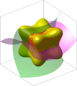
((c)) integration points in physical elements

Fig. 5: (a) Active, (black) elements in a background mesh are intersected by the shell midsurface, (b) integration points in one 3D reference element based on a (recursive) decomposition w.r.t. the master level-set function $\phi^{h}$ and further restriction to the slave level-set functions $\psi_{i}^{h}$, (c) integration points in the physical domain (red points) and integration points on the shell boundary (blue points).

4.1.2 Stabilization

Due to the restriction of the shape functions to the trace, see Eq. 4.2, the shape functions on the manifold only form a frame, which is, in general, not a basis [49, 45]. In Fig. 6, the consequences of the restriction to the trace of the manifold is visualized for a simple example.

Let us consider a 1D manifold (blue line) embedded in three bi-linear, quadrilateral 2D elements, see Fig. 6(a). Furthermore, a constant function on the manifold (black line) shall be interpolated based on the nodal values of the active background mesh. As shown in Fig. 6(b), the choice of the nodal values in order to interpolate the function on the manifold is not unique. In particular, three different configurations, which share the same values on the manifold are visualized.

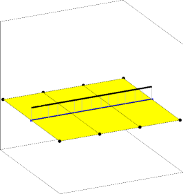
((a)) overview

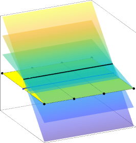
((b)) interpolation

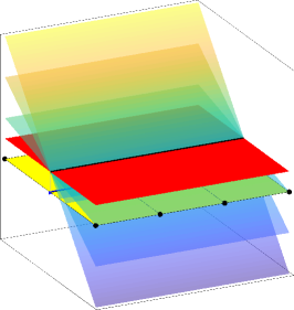
((c)) stabilization

Fig. 6: Background meshes do not uniquely define a (constant) function on the zero-level set: (a) The black line is a constant, scalar-valued function on the manifold (blue line), which is embedded in three, bi-linear quadrilateral background elements, (b) different possibilities for the interpolation of the function on the manifold (trace), (c) the stabilization adds a constraint in normal direction of the manifold resulting in a unique interpolation (red surface).

Therefore, a suitable stabilization term need to be added to the discrete weak form, otherwise the obtained linear system of equations does not have a unique solution w.r.t. the nodal values. In addition to the restriction, depending on unfavourable cut scenarios of cut background elements, unbounded small contributions to the stiffness matrix may occur, which causes an ill-conditioned system of linear equations.

The used stabilization technique addresses both issues and is introduced for scalar-valued problems in [30, 11]. This stabilization technique is called “normal derivative volume stabilization” and in [31, 43], the stabilization is applied to vector-valued problems. The stabilization term added to each unknown field in the discrete weak form is

$$s_{h}(\mathchoice{\displaystyle\bm{u}}{\textstyle\bm{u}}{\scriptstyle\bm{u}}{\scriptscriptstyle\bm{u}}^{h},\mathchoice{\displaystyle\bm{v}}{\textstyle\bm{v}}{\scriptstyle\bm{v}}{\scriptscriptstyle\bm{v}}^{h}):=\rho\int_{\Omega^{\Gamma}_{h}}\left(\nabla\mathchoice{\displaystyle\bm{u}}{\textstyle\bm{u}}{\scriptstyle\bm{u}}{\scriptscriptstyle\bm{u}}^{h}\cdot\mathchoice{\displaystyle\bm{n}}{\textstyle\bm{n}}{\scriptstyle\bm{n}}{\scriptscriptstyle\bm{n}}_{\Gamma}^{e,h}\right)\cdot\left(\nabla\mathchoice{\displaystyle\bm{v}}{\textstyle\bm{v}}{\scriptstyle\bm{v}}{\scriptscriptstyle\bm{v}}^{h}\cdot\mathchoice{\displaystyle\bm{n}}{\textstyle\bm{n}}{\scriptstyle\bm{n}}{\scriptscriptstyle\bm{n}}_{\Gamma}^{e,h}\right)\ \mathrm{d}V\ ,$$ (4.3)

where $\mathchoice{\displaystyle\bm{n}}{\textstyle\bm{n}}{\scriptstyle\bm{n}}{\scriptscriptstyle\bm{n}}_{\Gamma}^{e,h}(\mathchoice{\displaystyle\bm{x}}{\textstyle\bm{x}}{\scriptstyle\bm{x}}{\scriptscriptstyle\bm{x}})=\frac{\nabla\phi^{h}(\mathchoice{\displaystyle\bm{x}}{\textstyle\bm{x}}{\scriptstyle\bm{x}}{\scriptscriptstyle\bm{x}})}{\|\nabla\phi^{h}(\mathchoice{\displaystyle\bm{x}}{\textstyle\bm{x}}{\scriptstyle\bm{x}}{\scriptscriptstyle\bm{x}})\|},\mathchoice{\displaystyle\bm{x}}{\textstyle\bm{x}}{\scriptstyle\bm{x}}{\scriptscriptstyle\bm{x}}\in\Omega^{\Gamma}_{h}$ is a sufficiently smooth extension of the normal vector $\mathchoice{\displaystyle\bm{n}}{\textstyle\bm{n}}{\scriptstyle\bm{n}}{\scriptscriptstyle\bm{n}}_{\Gamma}^{h}$ at the zero-isosurface of $\phi^{h}$. It is noteworthy, that the integral is performed over the whole active background mesh and not restricted to the trace. However, the integrand is sufficiently smooth and, therefore, a standard numerical integration scheme w.r.t. the active elements is applicable, i.e., a standard 3D Gauss rule. By adding this constraint to the linear system of equations, the resulting system of equations features a unique solution, see Fig. 6(c). It is recommended in [30] that the stabilization parameter can be chosen within the following range

$$h\lesssim\rho\lesssim h^{-1}\ ,$$ (4.4)

where $h$ is the element size of the elements from the active mesh. This stabilization technique is suitable for higher-order shape functions, does not change the sparsity pattern of the stiffness matrix, and only first-order derivatives are needed. In addition, the implementation is straightforward and the choice of the stabilization parameter is rather flexible. Other stabilization techniques are presented in [45, 11]. A recent approach where two stabilizations techniques, i.e., face stabilization of the cut elements and the normal derivative stabilization on the zero-isosurface, are combined is presented in [39].

4.1.3 Essential boundary conditions

As outlined in [27], the enforcement of essential of boundary conditions is a challenging task in FDMs due to the fact that it is not possible to directly prescribe nodal values of the active background elements. The situation in the case of shells may be quite delicate due to complex boundary conditions, e.g., membrane support, symmetry support, clamped edges, etc., and, therefore, the treatment of boundary conditions requires special attention.

The essential (Dirichlet) boundary conditions may, in principle, be enforced in a weak manner using penalty methods, Lagrange multiplier methods, or Nitsche’s method. Herein, the non-symmetric version of Nitsche’s method is used to enforce the Dirichlet boundary conditions [7]. The advantage of this method in the context of FDMs is that it does not require additional stabilization terms and the discretization of auxiliary fields such as Lagrange multipliers is not needed. Furthermore, Nitsche’s method is a consistent approach to enforce essential boundary conditions, which may be an advantage if higher-order convergence rates shall be achieved. For further details about the non-symmetric version of Nitsche’s method we refer to, e.g., [7, 50, 32, 27]. The additional terms in the discrete weak form resulting from Nitsche’s method are presented in Section 4.2.2.

4.2 Discretization of the Reissner–Mindlin shell

In this section, the continuous weak form of the equilibrium, see Eq. 3.16 and Eq. 3.17 is discretized with the Trace FEM as described above. The discrete function spaces for the trial and test functions of the midsurface displacement field are

$$\mathcal{S}_{\mathchoice{\displaystyle\bm{u}}{\textstyle\bm{u}}{\scriptstyle\bm{u}}{\scriptscriptstyle\bm{u}}}^{h} =\left\{\mathchoice{\displaystyle\bm{u}}{\textstyle\bm{u}}{\scriptstyle\bm{u}}{\scriptscriptstyle\bm{u}}^{h}\in\left[\mathcal{T}_{h}\right]^{3}\right\}\ ,$$ (4.5)

$$\mathcal{V}_{\mathchoice{\displaystyle\bm{u}}{\textstyle\bm{u}}{\scriptstyle\bm{u}}{\scriptscriptstyle\bm{u}}}^{h} =\left\{\mathchoice{\displaystyle\bm{v}}{\textstyle\bm{v}}{\scriptstyle\bm{v}}{\scriptscriptstyle\bm{v}}_{u}^{h}\in\left[\mathcal{T}_{h}\right]^{3}\right\}\ .$$ (4.6)

For the stabilization of the discrete midsurface displacement, the above introduced normal derivative volume stabilization is employed. Regarding the discrete difference vector $\mathchoice{\displaystyle\bm{w}}{\textstyle\bm{w}}{\scriptstyle\bm{w}}{\scriptscriptstyle\bm{w}}^{h}$, the situation is more complicated due to the kinematic assumptions as the difference vector needs to be tangential. The discretization of tangent vector fields on implicitly defined manifolds is not straightforward and detailed in Section 4.2.1.

4.2.1 Discrete difference vector

Different approaches for the discretization of tangent vector fields are presented in, e.g., in [52, 43, 37]. Herein, the difference vector $\mathchoice{\displaystyle\bm{w}}{\textstyle\bm{w}}{\scriptstyle\bm{w}}{\scriptscriptstyle\bm{w}}^{h}$ and its corresponding test function $\mathchoice{\displaystyle\bm{v}}{\textstyle\bm{v}}{\scriptstyle\bm{v}}{\scriptscriptstyle\bm{v}}_{w}^{h}$ are defined in the general Trace FEM function space without the tangentiality constraint, similar to [43]. The corresponding function spaces are

$$\mathcal{S}_{\mathchoice{\displaystyle\bm{w}}{\textstyle\bm{w}}{\scriptstyle\bm{w}}{\scriptscriptstyle\bm{w}}}^{h} =\left\{\mathchoice{\displaystyle\bm{w}}{\textstyle\bm{w}}{\scriptstyle\bm{w}}{\scriptscriptstyle\bm{w}}^{h}\in\left[\mathcal{T}_{h}\right]^{3}\right\}\ ,$$ (4.7)

$$\mathcal{V}_{\mathchoice{\displaystyle\bm{w}}{\textstyle\bm{w}}{\scriptstyle\bm{w}}{\scriptscriptstyle\bm{w}}}^{h} =\left\{\mathchoice{\displaystyle\bm{v}}{\textstyle\bm{v}}{\scriptstyle\bm{v}}{\scriptscriptstyle\bm{v}}_{w}^{h}\in\left[\mathcal{T}_{h}\right]^{3}\right\}\ ,$$ (4.8)

but in the discrete weak form, see LABEL:eq:dwf and LABEL:eq:dwm, only the projected difference vector and test function are used, i.e., $\widetilde{\mathchoice{\displaystyle\bm{w}}{\textstyle\bm{w}}{\scriptstyle\bm{w}}{\scriptscriptstyle\bm{w}}}^{h}=\mathchoice{\displaystyle\mathbf{P}}{\textstyle\mathbf{P}}{\scriptstyle\mathbf{P}}{\scriptscriptstyle\mathbf{P}}\cdot\mathchoice{\displaystyle\bm{w}}{\textstyle\bm{w}}{\scriptstyle\bm{w}}{\scriptscriptstyle\bm{w}}^{h}\,,\ \widetilde{\mathchoice{\displaystyle\bm{v}}{\textstyle\bm{v}}{\scriptstyle\bm{v}}{\scriptscriptstyle\bm{v}}}_{w}^{h}=\mathchoice{\displaystyle\mathbf{P}}{\textstyle\mathbf{P}}{\scriptstyle\mathbf{P}}{\scriptscriptstyle\mathbf{P}}\cdot{\mathchoice{\displaystyle\bm{v}}{\textstyle\bm{v}}{\scriptstyle\bm{v}}{\scriptscriptstyle\bm{v}}_{w}}^{h}$. The directional and covariant gradient of the discrete, projected difference vector $\nabla_{\Gamma}^{\text{dir}}\widetilde{\mathchoice{\displaystyle\bm{w}}{\textstyle\bm{w}}{\scriptstyle\bm{w}}{\scriptscriptstyle\bm{w}}}^{h}$ and $\nabla_{\Gamma}^{\text{cov}}\widetilde{\mathchoice{\displaystyle\bm{w}}{\textstyle\bm{w}}{\scriptstyle\bm{w}}{\scriptscriptstyle\bm{w}}}^{h}$ can be directly computed with the product rule

$$\nabla_{\Gamma}^{\text{dir}}\widetilde{\mathchoice{\displaystyle\bm{w}}{\textstyle\bm{w}}{\scriptstyle\bm{w}}{\scriptscriptstyle\bm{w}}}^{h} =\nabla_{\Gamma}^{\text{dir}}\left(\mathchoice{\displaystyle\mathbf{P}}{\textstyle\mathbf{P}}{\scriptstyle\mathbf{P}}{\scriptscriptstyle\mathbf{P}}\cdot\mathchoice{\displaystyle\bm{w}}{\textstyle\bm{w}}{\scriptstyle\bm{w}}{\scriptscriptstyle\bm{w}}^{h}\right)=\begin{bmatrix}\nabla_{\Gamma\,x}^{\text{dir}}\mathchoice{\displaystyle\mathbf{P}}{\textstyle\mathbf{P}}{\scriptstyle\mathbf{P}}{\scriptscriptstyle\mathbf{P}}\cdot\mathchoice{\displaystyle\bm{w}}{\textstyle\bm{w}}{\scriptstyle\bm{w}}{\scriptscriptstyle\bm{w}}^{h}&\nabla_{\Gamma\,y}^{\text{dir}}\mathchoice{\displaystyle\mathbf{P}}{\textstyle\mathbf{P}}{\scriptstyle\mathbf{P}}{\scriptscriptstyle\mathbf{P}}\cdot\mathchoice{\displaystyle\bm{w}}{\textstyle\bm{w}}{\scriptstyle\bm{w}}{\scriptscriptstyle\bm{w}}^{h}&\nabla_{\Gamma\,z}^{\text{dir}}\mathchoice{\displaystyle\mathbf{P}}{\textstyle\mathbf{P}}{\scriptstyle\mathbf{P}}{\scriptscriptstyle\mathbf{P}}\cdot\mathchoice{\displaystyle\bm{w}}{\textstyle\bm{w}}{\scriptstyle\bm{w}}{\scriptscriptstyle\bm{w}}^{h}\end{bmatrix}+\nabla_{\Gamma}^{\text{cov}}\mathchoice{\displaystyle\bm{w}}{\textstyle\bm{w}}{\scriptstyle\bm{w}}{\scriptscriptstyle\bm{w}}^{h}\ ,$$ (4.9)

$$\nabla_{\Gamma}^{\text{cov}}\widetilde{\mathchoice{\displaystyle\bm{w}}{\textstyle\bm{w}}{\scriptstyle\bm{w}}{\scriptscriptstyle\bm{w}}}^{h} =\mathchoice{\displaystyle\mathbf{P}}{\textstyle\mathbf{P}}{\scriptstyle\mathbf{P}}{\scriptscriptstyle\mathbf{P}}\cdot\nabla_{\Gamma}^{\text{dir}}\widetilde{\mathchoice{\displaystyle\bm{w}}{\textstyle\bm{w}}{\scriptstyle\bm{w}}{\scriptscriptstyle\bm{w}}}^{h}=\mathchoice{\displaystyle\mathbf{P}}{\textstyle\mathbf{P}}{\scriptstyle\mathbf{P}}{\scriptscriptstyle\mathbf{P}}\cdot\begin{bmatrix}\nabla_{\Gamma\,x}^{\text{dir}}\mathchoice{\displaystyle\mathbf{P}}{\textstyle\mathbf{P}}{\scriptstyle\mathbf{P}}{\scriptscriptstyle\mathbf{P}}\cdot\mathchoice{\displaystyle\bm{w}}{\textstyle\bm{w}}{\scriptstyle\bm{w}}{\scriptscriptstyle\bm{w}}^{h}&\nabla_{\Gamma\,y}^{\text{dir}}\mathchoice{\displaystyle\mathbf{P}}{\textstyle\mathbf{P}}{\scriptstyle\mathbf{P}}{\scriptscriptstyle\mathbf{P}}\cdot\mathchoice{\displaystyle\bm{w}}{\textstyle\bm{w}}{\scriptstyle\bm{w}}{\scriptscriptstyle\bm{w}}^{h}&\nabla_{\Gamma\,z}^{\text{dir}}\mathchoice{\displaystyle\mathbf{P}}{\textstyle\mathbf{P}}{\scriptstyle\mathbf{P}}{\scriptscriptstyle\mathbf{P}}\cdot\mathchoice{\displaystyle\bm{w}}{\textstyle\bm{w}}{\scriptstyle\bm{w}}{\scriptscriptstyle\bm{w}}^{h}\end{bmatrix}+\nabla_{\Gamma}^{\text{cov}}\mathchoice{\displaystyle\bm{w}}{\textstyle\bm{w}}{\scriptstyle\bm{w}}{\scriptscriptstyle\bm{w}}^{h}\ .$$ (4.10)

One may argue that in this approach the derivatives of the projector $\mathchoice{\displaystyle\mathbf{P}}{\textstyle\mathbf{P}}{\scriptstyle\mathbf{P}}{\scriptscriptstyle\mathbf{P}}$ occur, which involves surface derivatives of the normal vector $\mathchoice{\displaystyle\bm{n}}{\textstyle\bm{n}}{\scriptstyle\bm{n}}{\scriptscriptstyle\bm{n}}_{\Gamma}^{h}$. This does not lead to additional computational costs, because in the case of the Reissner–Mindlin shell, the Weingarten map $\mathchoice{\displaystyle\mathbf{H}}{\textstyle\mathbf{H}}{\scriptstyle\mathbf{H}}{\scriptscriptstyle\mathbf{H}}$ directly appears in the weak form and, therefore, the surface derivatives of the normal vector $\mathchoice{\displaystyle\bm{n}}{\textstyle\bm{n}}{\scriptstyle\bm{n}}{\scriptscriptstyle\bm{n}}_{\Gamma}^{h}$ are required independently of this approach.

As a result of this projection, only the tangential part of $\mathchoice{\displaystyle\bm{w}}{\textstyle\bm{w}}{\scriptstyle\bm{w}}{\scriptscriptstyle\bm{w}}^{h}$ and $\mathchoice{\displaystyle\bm{v}}{\textstyle\bm{v}}{\scriptstyle\bm{v}}{\scriptscriptstyle\bm{v}}_{w}^{h}$ is considered in the discrete weak form and, therefore, the tangentiality constraint is built-in automatically. The employed stabilization technique, i.e., normal derivative volume stabilization, see Section 4.1.2, ensures unique nodal values and prevents an ill-conditioned system of equations due to small supports for general vector fields. However, due to the projection, the normal part of $\mathchoice{\displaystyle\bm{w}}{\textstyle\bm{w}}{\scriptstyle\bm{w}}{\scriptscriptstyle\bm{w}}^{h}$, i.e., $w^{h}_{n}=\mathchoice{\displaystyle\bm{w}}{\textstyle\bm{w}}{\scriptstyle\bm{w}}{\scriptscriptstyle\bm{w}}^{h}\cdot\mathchoice{\displaystyle\bm{n}}{\textstyle\bm{n}}{\scriptstyle\bm{n}}{\scriptscriptstyle\bm{n}}_{\Gamma}^{h}$, does not appear in the discrete weak form and, therefore, $\mathchoice{\displaystyle\bm{w}}{\textstyle\bm{w}}{\scriptstyle\bm{w}}{\scriptscriptstyle\bm{w}}^{h}_{n}$ is not unique. It is clear, that without any further measures this would lead to an ill-conditioned system of equations as a consequence. In order to address this issue, a simple and consistent additional stabilization term, similar to the penalty term in [43], is introduced

$$s_{w,h}:=\rho_{w}\int_{\Gamma^{h}}\left(\mathchoice{\displaystyle\bm{w}}{\textstyle\bm{w}}{\scriptstyle\bm{w}}{\scriptscriptstyle\bm{w}}^{h}\cdot\mathchoice{\displaystyle\bm{n}}{\textstyle\bm{n}}{\scriptstyle\bm{n}}{\scriptscriptstyle\bm{n}}_{\Gamma}^{h}\right)\left(\mathchoice{\displaystyle\bm{v}}{\textstyle\bm{v}}{\scriptstyle\bm{v}}{\scriptscriptstyle\bm{v}}_{w}^{h}\cdot\mathchoice{\displaystyle\bm{n}}{\textstyle\bm{n}}{\scriptstyle\bm{n}}{\scriptscriptstyle\bm{n}}_{\Gamma}^{h}\right)\ \mathrm{d}A\ ,$$ (4.11)

where $\rho_{w}$ is a suitable stabilization parameter. In other words, for the stabilization of the projected, discrete difference vector $\widetilde{\mathchoice{\displaystyle\bm{w}}{\textstyle\bm{w}}{\scriptstyle\bm{w}}{\scriptscriptstyle\bm{w}}}^{h}$, a combination of the normal derivative volume stabilization and the above introduced stabilization term for the normal part of $\mathchoice{\displaystyle\bm{w}}{\textstyle\bm{w}}{\scriptstyle\bm{w}}{\scriptscriptstyle\bm{w}}^{h}$ is employed, see LABEL:eq:dwm.

A series of numerical studies regarding the choice of the stabilization parameter $\rho_{w}$ for the Reissner–Mindlin shell has been conducted on flat and curved shell geometries. In detail, the dependency on the (1) material parameter $E$, (2) thickness $t$ and (3) element size on $h$ w.r.t. the condition number of the stiffness matrix and the influence on the results was investigated. Summarizing the outcome of the numerical studies, the stabilization parameter can be chosen independently of $h$ and for a suitable scaling of the stabilization term, the parameter is set to

$$\rho_{w}=E\cdot t\ .$$ (4.12)

A difference of the proposed approach and the method shown in [43] is that only the projected part of the vector field, i.e., $\widetilde{\mathchoice{\displaystyle\bm{w}}{\textstyle\bm{w}}{\scriptstyle\bm{w}}{\scriptscriptstyle\bm{w}}}^{h}=\mathchoice{\displaystyle\mathbf{P}}{\textstyle\mathbf{P}}{\scriptstyle\mathbf{P}}{\scriptscriptstyle\mathbf{P}}\cdot\mathchoice{\displaystyle\bm{w}}{\textstyle\bm{w}}{\scriptstyle\bm{w}}{\scriptscriptstyle\bm{w}}^{h}$, is used in the discrete weak form which directly enforces the tangentiality constraint. Furthermore, the used stabilization parameter, which is in [43, 37] a penalty parameter, does not depend on $h$ and only a suitable scaling of the stabilization term may be required.

4.2.2 Discrete weak form

Based on the previous definitions, the discrete weak form with the Trace FEM of the force equilibrium, see Eq. 3.16, reads as follows: Given material parameters $(E,\nu)\in\mathbb{R}^{+}$, body forces $\mathchoice{\displaystyle\bm{f}}{\textstyle\bm{f}}{\scriptstyle\bm{f}}{\scriptscriptstyle\bm{f}}\in\mathbb{R}^{3}$ on $\Gamma^{h}$, tractions $\hat{\mathchoice{\displaystyle\bm{p}}{\textstyle\bm{p}}{\scriptstyle\bm{p}}{\scriptscriptstyle\bm{p}}}$ on $\partial\Gamma^{h}_{\text{N},\mathchoice{\displaystyle\bm{u}}{\textstyle\bm{u}}{\scriptstyle\bm{u}}{\scriptscriptstyle\bm{u}}}$, stabilization parameter $\rho\in\mathbb{R}^{+}$ find the displacement fields $(\mathchoice{\displaystyle\bm{u}}{\textstyle\bm{u}}{\scriptstyle\bm{u}}{\scriptscriptstyle\bm{u}}^{h},\mathchoice{\displaystyle\bm{w}}{\textstyle\bm{w}}{\scriptstyle\bm{w}}{\scriptscriptstyle\bm{w}}^{h})\in\mathcal{S}_{\mathchoice{\displaystyle\bm{u}}{\textstyle\bm{u}}{\scriptstyle\bm{u}}{\scriptscriptstyle\bm{u}}}^{h}\times\mathcal{S}_{\mathchoice{\displaystyle\bm{w}}{\textstyle\bm{w}}{\scriptstyle\bm{w}}{\scriptscriptstyle\bm{w}}}^{h}$ such that for all test functions $(\mathchoice{\displaystyle\bm{v}}{\textstyle\bm{v}}{\scriptstyle\bm{v}}{\scriptscriptstyle\bm{v}}_{u}^{h},\mathchoice{\displaystyle\bm{v}}{\textstyle\bm{v}}{\scriptstyle\bm{v}}{\scriptscriptstyle\bm{v}}_{w}^{h})\in\mathcal{V}_{\mathchoice{\displaystyle\bm{u}}{\textstyle\bm{u}}{\scriptstyle\bm{u}}{\scriptscriptstyle\bm{u}}}^{h}\times\mathcal{V}_{\mathchoice{\displaystyle\bm{w}}{\textstyle\bm{w}}{\scriptstyle\bm{w}}{\scriptscriptstyle\bm{w}}}^{h}$ there holds in $\Gamma^{h}$

$$\begin{split}&\int_{\Gamma^{h}}\nabla_{\Gamma}^{\text{dir}}\mathchoice{\displaystyle\bm{v}}{\textstyle\bm{v}}{\scriptstyle\bm{v}}{\scriptscriptstyle\bm{v}}_{u}:\tilde{\mathchoice{\displaystyle\mathbf{n}}{\textstyle\mathbf{n}}{\scriptstyle\mathbf{n}}{\scriptscriptstyle\mathbf{n}}}_{\Gamma}(\mathchoice{\displaystyle\bm{u}}{\textstyle\bm{u}}{\scriptstyle\bm{u}}{\scriptscriptstyle\bm{u}}^{h})+(\mathchoice{\displaystyle\mathbf{H}}{\textstyle\mathbf{H}}{\scriptstyle\mathbf{H}}{\scriptscriptstyle\mathbf{H}}\cdot\nabla_{\Gamma}^{\text{dir}}\mathchoice{\displaystyle\bm{v}}{\textstyle\bm{v}}{\scriptstyle\bm{v}}{\scriptscriptstyle\bm{v}}_{u}):\mathchoice{\displaystyle\mathbf{m}}{\textstyle\mathbf{m}}{\scriptstyle\mathbf{m}}{\scriptscriptstyle\mathbf{m}}_{\Gamma}(\mathchoice{\displaystyle\bm{u}}{\textstyle\bm{u}}{\scriptstyle\bm{u}}{\scriptscriptstyle\bm{u}}^{h},\widetilde{\mathchoice{\displaystyle\bm{w}}{\textstyle\bm{w}}{\scriptstyle\bm{w}}{\scriptscriptstyle\bm{w}}}^{h})+(\mathchoice{\displaystyle\mathbf{Q}}{\textstyle\mathbf{Q}}{\scriptstyle\mathbf{Q}}{\scriptscriptstyle\mathbf{Q}}\cdot\nabla_{\Gamma}^{\text{dir}}\mathchoice{\displaystyle\bm{v}}{\textstyle\bm{v}}{\scriptstyle\bm{v}}{\scriptscriptstyle\bm{v}}_{u}):\mathchoice{\displaystyle\mathbf{q}}{\textstyle\mathbf{q}}{\scriptstyle\mathbf{q}}{\scriptscriptstyle\mathbf{q}}_{\Gamma}(\mathchoice{\displaystyle\bm{u}}{\textstyle\bm{u}}{\scriptstyle\bm{u}}{\scriptscriptstyle\bm{u}}^{h},\widetilde{\mathchoice{\displaystyle\bm{w}}{\textstyle\bm{w}}{\scriptstyle\bm{w}}{\scriptscriptstyle\bm{w}}}^{h})\ \mathrm{d}A\\[7.11317pt] &-\underbrace{\int_{\partial\Gamma_{\text{D},\mathchoice{\displaystyle\bm{u}}{\textstyle\bm{u}}{\scriptstyle\bm{u}}{\scriptscriptstyle\bm{u}}}^{h}}\mathchoice{\displaystyle\bm{v}}{\textstyle\bm{v}}{\scriptstyle\bm{v}}{\scriptscriptstyle\bm{v}}_{u}\cdot\mathchoice{\displaystyle\bm{p}}{\textstyle\bm{p}}{\scriptstyle\bm{p}}{\scriptscriptstyle\bm{p}}(\mathchoice{\displaystyle\bm{u}}{\textstyle\bm{u}}{\scriptstyle\bm{u}}{\scriptscriptstyle\bm{u}}^{h},\widetilde{\mathchoice{\displaystyle\bm{w}}{\textstyle\bm{w}}{\scriptstyle\bm{w}}{\scriptscriptstyle\bm{w}}}^{h})\ \mathrm{d}s}_{\text{boundary term due to\ }\mathchoice{\displaystyle\bm{v}}{\textstyle\bm{v}}{\scriptstyle\bm{v}}{\scriptscriptstyle\bm{v}}_{u}^{h}\neq\mathchoice{\displaystyle\bm{0}}{\textstyle\bm{0}}{\scriptstyle\bm{0}}{\scriptscriptstyle\bm{0}}\text{ on }\partial\Gamma_{\text{D},\mathchoice{\displaystyle\bm{u}}{\textstyle\bm{u}}{\scriptstyle\bm{u}}{\scriptscriptstyle\bm{u}}}}+\underbrace{\int_{\partial\Gamma_{\text{D},\mathchoice{\displaystyle\bm{u}}{\textstyle\bm{u}}{\scriptstyle\bm{u}}{\scriptscriptstyle\bm{u}}}^{h}}\mathchoice{\displaystyle\bm{u}}{\textstyle\bm{u}}{\scriptstyle\bm{u}}{\scriptscriptstyle\bm{u}}^{h}\cdot\mathchoice{\displaystyle\bm{p}}{\textstyle\bm{p}}{\scriptstyle\bm{p}}{\scriptscriptstyle\bm{p}}(\mathchoice{\displaystyle\bm{v}}{\textstyle\bm{v}}{\scriptstyle\bm{v}}{\scriptscriptstyle\bm{v}}_{u}^{h},\widetilde{\mathchoice{\displaystyle\bm{v}}{\textstyle\bm{v}}{\scriptstyle\bm{v}}{\scriptscriptstyle\bm{v}}}_{w}^{h})\ \mathrm{d}s}_{\text{Nitsche term for displ.\leavevmode\nobreak\ on LHS}}\\[7.11317pt] &+\underbrace{\rho\int_{\Omega^{\Gamma}_{h}}\left(\nabla\mathchoice{\displaystyle\bm{u}}{\textstyle\bm{u}}{\scriptstyle\bm{u}}{\scriptscriptstyle\bm{u}}^{h}\cdot\mathchoice{\displaystyle\bm{n}}{\textstyle\bm{n}}{\scriptstyle\bm{n}}{\scriptscriptstyle\bm{n}}_{\Gamma}^{e,h}\right)\cdot\left(\nabla\mathchoice{\displaystyle\bm{v}}{\textstyle\bm{v}}{\scriptstyle\bm{v}}{\scriptscriptstyle\bm{v}}_{u}^{h}\cdot\mathchoice{\displaystyle\bm{n}}{\textstyle\bm{n}}{\scriptstyle\bm{n}}{\scriptscriptstyle\bm{n}}_{\Gamma}^{e,h}\right)\ \mathrm{d}V}_{\text{Trace FEM stabilization, see \autoref{sec:stab}}}\\[7.11317pt] &=\int_{\Gamma^{h}}\mathchoice{\displaystyle\bm{v}}{\textstyle\bm{v}}{\scriptstyle\bm{v}}{\scriptscriptstyle\bm{v}}_{u}^{h}\cdot\mathchoice{\displaystyle\bm{f}}{\textstyle\bm{f}}{\scriptstyle\bm{f}}{\scriptscriptstyle\bm{f}}\ \mathrm{d}A+\underbrace{\int_{\partial\Gamma_{\text{D},\mathchoice{\displaystyle\bm{u}}{\textstyle\bm{u}}{\scriptstyle\bm{u}}{\scriptscriptstyle\bm{u}}}^{h}}\hat{\mathchoice{\displaystyle\bm{g}}{\textstyle\bm{g}}{\scriptstyle\bm{g}}{\scriptscriptstyle\bm{g}}}_{\mathchoice{\displaystyle\bm{u}}{\textstyle\bm{u}}{\scriptstyle\bm{u}}{\scriptscriptstyle\bm{u}}}\cdot\mathchoice{\displaystyle\bm{p}}{\textstyle\bm{p}}{\scriptstyle\bm{p}}{\scriptscriptstyle\bm{p}}(\mathchoice{\displaystyle\bm{v}}{\textstyle\bm{v}}{\scriptstyle\bm{v}}{\scriptscriptstyle\bm{v}}_{u}^{h},\widetilde{\mathchoice{\displaystyle\bm{v}}{\textstyle\bm{v}}{\scriptstyle\bm{v}}{\scriptscriptstyle\bm{v}}}_{w}^{h})\ \mathrm{d}s}_{\text{Nitsche term for displ.\leavevmode\nobreak\ on RHS}}+\int_{\partial\Gamma_{\text{N},\mathchoice{\displaystyle\bm{u}}{\textstyle\bm{u}}{\scriptstyle\bm{u}}{\scriptscriptstyle\bm{u}}}^{h}}\mathchoice{\displaystyle\bm{v}}{\textstyle\bm{v}}{\scriptstyle\bm{v}}{\scriptscriptstyle\bm{v}}_{u}^{h}\cdot\hat{\mathchoice{\displaystyle\bm{p}}{\textstyle\bm{p}}{\scriptstyle\bm{p}}{\scriptscriptstyle\bm{p}}}\ \mathrm{d}s\ ,\end{split}$$ (4.13)

where $\mathchoice{\displaystyle\bm{p}}{\textstyle\bm{p}}{\scriptstyle\bm{p}}{\scriptscriptstyle\bm{p}}=\mathchoice{\displaystyle\mathbf{n}}{\textstyle\mathbf{n}}{\scriptstyle\mathbf{n}}{\scriptscriptstyle\mathbf{n}}_{\Gamma}^{\text{real}}\cdot\mathchoice{\displaystyle\bm{n}}{\textstyle\bm{n}}{\scriptstyle\bm{n}}{\scriptscriptstyle\bm{n}}_{\partial\Gamma}^{h}+\left(\mathchoice{\displaystyle\bm{n}}{\textstyle\bm{n}}{\scriptstyle\bm{n}}{\scriptscriptstyle\bm{n}}_{\Gamma}^{h}\cdot\mathchoice{\displaystyle\mathbf{q}}{\textstyle\mathbf{q}}{\scriptstyle\mathbf{q}}{\scriptscriptstyle\mathbf{q}}_{\Gamma}\cdot\mathchoice{\displaystyle\bm{n}}{\textstyle\bm{n}}{\scriptstyle\bm{n}}{\scriptscriptstyle\bm{n}}_{\partial\Gamma}^{h}\right)\mathchoice{\displaystyle\bm{n}}{\textstyle\bm{n}}{\scriptstyle\bm{n}}{\scriptscriptstyle\bm{n}}_{\Gamma}^{h}$, see Eq. 3.11, are the conjugated forces at the Dirichlet boundary $\partial\Gamma_{\text{D},\mathchoice{\displaystyle\bm{u}}{\textstyle\bm{u}}{\scriptstyle\bm{u}}{\scriptscriptstyle\bm{u}}}^{h}$.

The discrete weak form of the moment equilibrium, see Eq. 3.17 reads as follows: Given material parameters $(E,\nu)\in\mathbb{R}^{+}$, distributed moments $\mathchoice{\displaystyle\bm{c}}{\textstyle\bm{c}}{\scriptstyle\bm{c}}{\scriptscriptstyle\bm{c}}\in T_{P}\Gamma^{h}$ on $\Gamma^{h}$, bending moments $\hat{\mathchoice{\displaystyle\bm{m}}{\textstyle\bm{m}}{\scriptstyle\bm{m}}{\scriptscriptstyle\bm{m}}}_{\partial\Gamma}$ on $\partial\Gamma^{h}_{\text{N},\mathchoice{\displaystyle\bm{w}}{\textstyle\bm{w}}{\scriptstyle\bm{w}}{\scriptscriptstyle\bm{w}}}$, stabilization parameters $(\rho,\rho_{w})\in\mathbb{R}^{+}$ find the displacement fields $(\mathchoice{\displaystyle\bm{u}}{\textstyle\bm{u}}{\scriptstyle\bm{u}}{\scriptscriptstyle\bm{u}}^{h},\mathchoice{\displaystyle\bm{w}}{\textstyle\bm{w}}{\scriptstyle\bm{w}}{\scriptscriptstyle\bm{w}}^{h})\in\mathcal{S}_{\mathchoice{\displaystyle\bm{u}}{\textstyle\bm{u}}{\scriptstyle\bm{u}}{\scriptscriptstyle\bm{u}}}^{h}\times\mathcal{S}_{\mathchoice{\displaystyle\bm{w}}{\textstyle\bm{w}}{\scriptstyle\bm{w}}{\scriptscriptstyle\bm{w}}}^{h}$ such that for all test functions $(\mathchoice{\displaystyle\bm{v}}{\textstyle\bm{v}}{\scriptstyle\bm{v}}{\scriptscriptstyle\bm{v}}_{u}^{h},\mathchoice{\displaystyle\bm{v}}{\textstyle\bm{v}}{\scriptstyle\bm{v}}{\scriptscriptstyle\bm{v}}_{w}^{h})\in\mathcal{V}_{\mathchoice{\displaystyle\bm{u}}{\textstyle\bm{u}}{\scriptstyle\bm{u}}{\scriptscriptstyle\bm{u}}}^{h}\times\mathcal{V}_{\mathchoice{\displaystyle\bm{w}}{\textstyle\bm{w}}{\scriptstyle\bm{w}}{\scriptscriptstyle\bm{w}}}^{h}$ there holds in $\Gamma^{h}$

$$\begin{split}&\int_{\Gamma^{h}}\nabla_{\Gamma}^{\text{dir}}\widetilde{\mathchoice{\displaystyle\bm{v}}{\textstyle\bm{v}}{\scriptstyle\bm{v}}{\scriptscriptstyle\bm{v}}}_{w}^{h}:\mathchoice{\displaystyle\mathbf{m}}{\textstyle\mathbf{m}}{\scriptstyle\mathbf{m}}{\scriptscriptstyle\mathbf{m}}_{\Gamma}(\mathchoice{\displaystyle\bm{u}}{\textstyle\bm{u}}{\scriptstyle\bm{u}}{\scriptscriptstyle\bm{u}}^{h},\widetilde{\mathchoice{\displaystyle\bm{w}}{\textstyle\bm{w}}{\scriptstyle\bm{w}}{\scriptscriptstyle\bm{w}}}^{h})+\widetilde{\mathchoice{\displaystyle\bm{v}}{\textstyle\bm{v}}{\scriptstyle\bm{v}}{\scriptscriptstyle\bm{v}}}_{w}^{h}\cdot\left[\mathchoice{\displaystyle\mathbf{q}}{\textstyle\mathbf{q}}{\scriptstyle\mathbf{q}}{\scriptscriptstyle\mathbf{q}}_{\Gamma}(\mathchoice{\displaystyle\bm{u}}{\textstyle\bm{u}}{\scriptstyle\bm{u}}{\scriptscriptstyle\bm{u}}^{h},\widetilde{\mathchoice{\displaystyle\bm{w}}{\textstyle\bm{w}}{\scriptstyle\bm{w}}{\scriptscriptstyle\bm{w}}}^{h})\cdot\mathchoice{\displaystyle\bm{n}}{\textstyle\bm{n}}{\scriptstyle\bm{n}}{\scriptscriptstyle\bm{n}}_{\Gamma}\right]\ \mathrm{d}A\\[7.11317pt] &-\underbrace{\int_{\partial\Gamma_{\text{D},\mathchoice{\displaystyle\bm{w}}{\textstyle\bm{w}}{\scriptstyle\bm{w}}{\scriptscriptstyle\bm{w}}}}\widetilde{\mathchoice{\displaystyle\bm{v}}{\textstyle\bm{v}}{\scriptstyle\bm{v}}{\scriptscriptstyle\bm{v}}}_{w}^{h}\cdot\mathchoice{\displaystyle\bm{m}}{\textstyle\bm{m}}{\scriptstyle\bm{m}}{\scriptscriptstyle\bm{m}}_{\partial\Gamma}(\mathchoice{\displaystyle\bm{u}}{\textstyle\bm{u}}{\scriptstyle\bm{u}}{\scriptscriptstyle\bm{u}}^{h},\widetilde{\mathchoice{\displaystyle\bm{w}}{\textstyle\bm{w}}{\scriptstyle\bm{w}}{\scriptscriptstyle\bm{w}}}^{h})\ \mathrm{d}s}_{\text{boundary term due to\ }\mathchoice{\displaystyle\bm{v}}{\textstyle\bm{v}}{\scriptstyle\bm{v}}{\scriptscriptstyle\bm{v}}_{w}^{h}\neq\mathchoice{\displaystyle\bm{0}}{\textstyle\bm{0}}{\scriptstyle\bm{0}}{\scriptscriptstyle\bm{0}}\text{ on }\partial\Gamma_{\text{D},\mathchoice{\displaystyle\bm{w}}{\textstyle\bm{w}}{\scriptstyle\bm{w}}{\scriptscriptstyle\bm{w}}}}+\underbrace{\int_{\partial\Gamma_{\text{D},\mathchoice{\displaystyle\bm{w}}{\textstyle\bm{w}}{\scriptstyle\bm{w}}{\scriptscriptstyle\bm{w}}}}\widetilde{\mathchoice{\displaystyle\bm{w}}{\textstyle\bm{w}}{\scriptstyle\bm{w}}{\scriptscriptstyle\bm{w}}}^{h}\cdot\mathchoice{\displaystyle\bm{m}}{\textstyle\bm{m}}{\scriptstyle\bm{m}}{\scriptscriptstyle\bm{m}}_{\partial\Gamma}(\mathchoice{\displaystyle\bm{v}}{\textstyle\bm{v}}{\scriptstyle\bm{v}}{\scriptscriptstyle\bm{v}}_{u}^{h},\widetilde{\mathchoice{\displaystyle\bm{v}}{\textstyle\bm{v}}{\scriptstyle\bm{v}}{\scriptscriptstyle\bm{v}}}_{w}^{h})\ \mathrm{d}s}_{\text{Nitsche term for rot.\leavevmode\nobreak\ on LHS}}\\[7.11317pt] &+\underbrace{\rho\int_{\Omega^{\Gamma}_{h}}\left(\nabla\mathchoice{\displaystyle\bm{w}}{\textstyle\bm{w}}{\scriptstyle\bm{w}}{\scriptscriptstyle\bm{w}}^{h}\cdot\mathchoice{\displaystyle\bm{n}}{\textstyle\bm{n}}{\scriptstyle\bm{n}}{\scriptscriptstyle\bm{n}}_{\Gamma}^{e,h}\right)\cdot\left(\nabla\mathchoice{\displaystyle\bm{v}}{\textstyle\bm{v}}{\scriptstyle\bm{v}}{\scriptscriptstyle\bm{v}}_{w}^{h}\cdot\mathchoice{\displaystyle\bm{n}}{\textstyle\bm{n}}{\scriptstyle\bm{n}}{\scriptscriptstyle\bm{n}}_{\Gamma}^{e,h}\right)\ \mathrm{d}V}_{\text{Trace FEM stabilization, see \autoref{sec:stab}}}+\underbrace{\rho_{w}\int_{\Gamma^{h}}\left(\mathchoice{\displaystyle\bm{w}}{\textstyle\bm{w}}{\scriptstyle\bm{w}}{\scriptscriptstyle\bm{w}}^{h}\cdot\mathchoice{\displaystyle\bm{n}}{\textstyle\bm{n}}{\scriptstyle\bm{n}}{\scriptscriptstyle\bm{n}}_{\Gamma}^{h}\right)\left(\mathchoice{\displaystyle\bm{v}}{\textstyle\bm{v}}{\scriptstyle\bm{v}}{\scriptscriptstyle\bm{v}}_{w}^{h}\cdot\mathchoice{\displaystyle\bm{n}}{\textstyle\bm{n}}{\scriptstyle\bm{n}}{\scriptscriptstyle\bm{n}}_{\Gamma}^{h}\right)\ \mathrm{d}A}_{\text{stabilization term for\ }\widetilde{\mathchoice{\displaystyle\bm{w}}{\textstyle\bm{w}}{\scriptstyle\bm{w}}{\scriptscriptstyle\bm{w}}}^{h}\text{\ see \autoref{sec:discdiffvec}}}\\[7.11317pt] &=\int_{\Gamma^{h}}\mathchoice{\displaystyle\bm{v}}{\textstyle\bm{v}}{\scriptstyle\bm{v}}{\scriptscriptstyle\bm{v}}_{w}^{h}\cdot\mathchoice{\displaystyle\bm{c}}{\textstyle\bm{c}}{\scriptstyle\bm{c}}{\scriptscriptstyle\bm{c}}\ \mathrm{d}A+\underbrace{\int_{\partial\Gamma_{\text{D},\mathchoice{\displaystyle\bm{w}}{\textstyle\bm{w}}{\scriptstyle\bm{w}}{\scriptscriptstyle\bm{w}}}^{h}}\hat{\mathchoice{\displaystyle\bm{g}}{\textstyle\bm{g}}{\scriptstyle\bm{g}}{\scriptscriptstyle\bm{g}}}_{\mathchoice{\displaystyle\bm{w}}{\textstyle\bm{w}}{\scriptstyle\bm{w}}{\scriptscriptstyle\bm{w}}}\cdot\mathchoice{\displaystyle\bm{m}}{\textstyle\bm{m}}{\scriptstyle\bm{m}}{\scriptscriptstyle\bm{m}}_{\partial\Gamma}(\mathchoice{\displaystyle\bm{v}}{\textstyle\bm{v}}{\scriptstyle\bm{v}}{\scriptscriptstyle\bm{v}}_{u}^{h},\widetilde{\mathchoice{\displaystyle\bm{v}}{\textstyle\bm{v}}{\scriptstyle\bm{v}}{\scriptscriptstyle\bm{v}}}_{w}^{h})\ \mathrm{d}s}_{\text{Nitsche term for rot.\leavevmode\nobreak\ on RHS}}+\int_{\partial\Gamma_{\text{N},\mathchoice{\displaystyle\bm{w}}{\textstyle\bm{w}}{\scriptstyle\bm{w}}{\scriptscriptstyle\bm{w}}}^{h}}\mathchoice{\displaystyle\bm{v}}{\textstyle\bm{v}}{\scriptstyle\bm{v}}{\scriptscriptstyle\bm{v}}_{w}^{h}\cdot\hat{\mathchoice{\displaystyle\bm{m}}{\textstyle\bm{m}}{\scriptstyle\bm{m}}{\scriptscriptstyle\bm{m}}_{\partial\Gamma}}\ \mathrm{d}s\ ,\end{split}$$ (4.14)

where $\mathchoice{\displaystyle\bm{m}}{\textstyle\bm{m}}{\scriptstyle\bm{m}}{\scriptscriptstyle\bm{m}}_{\partial\Gamma}=\mathchoice{\displaystyle\mathbf{m}}{\textstyle\mathbf{m}}{\scriptstyle\mathbf{m}}{\scriptscriptstyle\mathbf{m}}_{\Gamma}\cdot\mathchoice{\displaystyle\bm{n}}{\textstyle\bm{n}}{\scriptstyle\bm{n}}{\scriptscriptstyle\bm{n}}_{\partial\Gamma}^{h}$, see Eq. 3.11, are the conjugated bending moments at the Dirichlet boundary $\partial\Gamma_{\text{D},\mathchoice{\displaystyle\bm{w}}{\textstyle\bm{w}}{\scriptstyle\bm{w}}{\scriptscriptstyle\bm{w}}}^{h}$. Note that in the implementation one may employ the identity $\mathchoice{\displaystyle\mathbf{A}}{\textstyle\mathbf{A}}{\scriptstyle\mathbf{A}}{\scriptscriptstyle\mathbf{A}}:\mathchoice{\displaystyle\mathbf{B}}{\textstyle\mathbf{B}}{\scriptstyle\mathbf{B}}{\scriptscriptstyle\mathbf{B}}=(\mathchoice{\displaystyle\mathbf{P}}{\textstyle\mathbf{P}}{\scriptstyle\mathbf{P}}{\scriptscriptstyle\mathbf{P}}\cdot\mathchoice{\displaystyle\mathbf{A}}{\textstyle\mathbf{A}}{\scriptstyle\mathbf{A}}{\scriptscriptstyle\mathbf{A}}\cdot\mathchoice{\displaystyle\mathbf{P}}{\textstyle\mathbf{P}}{\scriptstyle\mathbf{P}}{\scriptscriptstyle\mathbf{P}}):\mathchoice{\displaystyle\mathbf{B}}{\textstyle\mathbf{B}}{\scriptstyle\mathbf{B}}{\scriptscriptstyle\mathbf{B}}^{\text{dir}}$ with $(\mathchoice{\displaystyle\mathbf{A}}{\textstyle\mathbf{A}}{\scriptstyle\mathbf{A}}{\scriptscriptstyle\mathbf{A}},\mathchoice{\displaystyle\mathbf{B}}{\textstyle\mathbf{B}}{\scriptstyle\mathbf{B}}{\scriptscriptstyle\mathbf{B}})\in\mathbb{R}^{3\times 3}$ and $\mathchoice{\displaystyle\mathbf{B}}{\textstyle\mathbf{B}}{\scriptstyle\mathbf{B}}{\scriptscriptstyle\mathbf{B}}=\mathchoice{\displaystyle\mathbf{P}}{\textstyle\mathbf{P}}{\scriptstyle\mathbf{P}}{\scriptscriptstyle\mathbf{P}}\cdot\mathchoice{\displaystyle\mathbf{B}}{\textstyle\mathbf{B}}{\scriptstyle\mathbf{B}}{\scriptscriptstyle\mathbf{B}}^{\text{dir}}\cdot\mathchoice{\displaystyle\mathbf{P}}{\textstyle\mathbf{P}}{\scriptstyle\mathbf{P}}{\scriptscriptstyle\mathbf{P}}$ in order to further simplify the obtained terms with the projected difference vector. As a result, only directional derivatives of the discrete, projected difference vector are required which simplifies the implementation significantly.

The usual element assembly w.r.t. the active elements yields a linear system of equations in the following form

$$\underbrace{\left(\mathchoice{\displaystyle\mathbf{K}}{\textstyle\mathbf{K}}{\scriptstyle\mathbf{K}}{\scriptscriptstyle\mathbf{K}}_{\text{Stiff}}+\mathchoice{\displaystyle\mathbf{K}}{\textstyle\mathbf{K}}{\scriptstyle\mathbf{K}}{\scriptscriptstyle\mathbf{K}}_{\text{Nitsche}}+\mathchoice{\displaystyle\mathbf{K}}{\textstyle\mathbf{K}}{\scriptstyle\mathbf{K}}{\scriptscriptstyle\mathbf{K}}_{\text{Stab}}\right)}_{\mathchoice{\displaystyle\mathbf{K}}{\textstyle\mathbf{K}}{\scriptstyle\mathbf{K}}{\scriptscriptstyle\mathbf{K}}}\cdot\begin{bmatrix}\underline{\hat{\mathchoice{\displaystyle\bm{u}}{\textstyle\bm{u}}{\scriptstyle\bm{u}}{\scriptscriptstyle\bm{u}}}}\\ \underline{\hat{\mathchoice{\displaystyle\bm{w}}{\textstyle\bm{w}}{\scriptstyle\bm{w}}{\scriptscriptstyle\bm{w}}}}\end{bmatrix} =\underbrace{\left(\mathchoice{\displaystyle\bm{b}}{\textstyle\bm{b}}{\scriptstyle\bm{b}}{\scriptscriptstyle\bm{b}}_{\text{Load}}+\mathchoice{\displaystyle\bm{b}}{\textstyle\bm{b}}{\scriptstyle\bm{b}}{\scriptscriptstyle\bm{b}}_{\text{Nitsche}}\right)}_{\mathchoice{\displaystyle\bm{b}}{\textstyle\bm{b}}{\scriptstyle\bm{b}}{\scriptscriptstyle\bm{b}}}\ ,$$ (4.15)

with $[\underline{\hat{\mathchoice{\displaystyle\bm{u}}{\textstyle\bm{u}}{\scriptstyle\bm{u}}{\scriptscriptstyle\bm{u}}}},\underline{\hat{\mathchoice{\displaystyle\bm{w}}{\textstyle\bm{w}}{\scriptstyle\bm{w}}{\scriptscriptstyle\bm{w}}}}]$ being the sought displacements and rotations of the normal vector at the nodes of the active elements. The matrix $\mathchoice{\displaystyle\mathbf{K}}{\textstyle\mathbf{K}}{\scriptstyle\mathbf{K}}{\scriptscriptstyle\mathbf{K}}$ and the load vector $\mathchoice{\displaystyle\bm{b}}{\textstyle\bm{b}}{\scriptstyle\bm{b}}{\scriptscriptstyle\bm{b}}$ are split into: (1) standard terms for the stiffness matrix, (2) boundary terms, (3) stabilization terms, respectively.

5 Numerical results

In this section, the proposed numerical method for implicitly defined Reissner–Mindlin shells is tested on a set of benchmark examples, consisting of the partly clamped hyperbolic parabolid from [2, 14], the partly clamped gyroid from [28] and a clamped flower-shaped shell inspired by [51, 52]. In the case of the first two examples the shells are rather thin and locking phenomena can be expected, especially in the case of low ansatz orders. However, when increasing the order $p$, locking phenomena decrease significantly and, therefore, no further measures against locking phenomena are considered herein.

In the convergence studies, quasi-regular background meshes consisting of tetrahedral elements are used. For all unknown fields, i.e., $\mathchoice{\displaystyle\bm{u}}{\textstyle\bm{u}}{\scriptstyle\bm{u}}{\scriptscriptstyle\bm{u}}^{h},\mathchoice{\displaystyle\bm{w}}{\textstyle\bm{w}}{\scriptstyle\bm{w}}{\scriptscriptstyle\bm{w}}^{h}$, and the interpolation of the level-set functions, the same order of shape functions are used. The orders are varied as $2\leq p\leq 6$. The element size $h$ is proportional to the factor $n$ which is related to the number of elements and is varied between $2\leq n\leq 128$.

In the presented examples, the stabilization parameter $\rho$ for the normal derivative volume stabilization is set to $\rho=\nicefrac{{1000}}{{h}}$. In order to achieve a proper scaling of the stiffness matrix, the parameter $\rho_{w}$, is set to $\rho_{w}=Et$, as proposed in Section 4.2.1.

5.1 Hyperbolic paraboloid

The first example is the partly clamped hyperbolic paraboloid and is taken from [2, 14]. The problem is defined in Fig. 7. The yellow surface is the zero-isosurface of the master level-set function $\phi$ and the grey planes are the zero-isosurfaces of the slave level-set functions $\psi_{j},\ j\in[1,4]$, which define the boundaries of the shell. The blue line is the clamped edge of the shell.

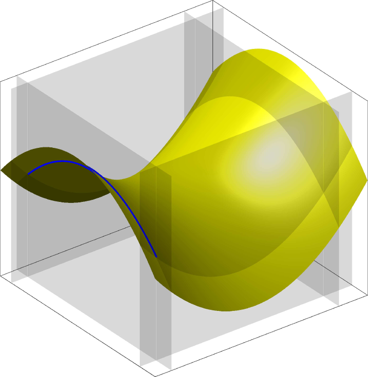
Fig. 7: Definition of the partly clamped hyperbolic paraboloid problem.

In Fig. 8(a), the active background mesh which contains only cut elements with $p=4$ is shown. In Fig. 8(b), the corresponding integration points are illustrated, those in the domain are plotted in red and those on the boundaries are blue. In Fig. 8(c), the numerical solution of the partly clamped hyperbolic paraboloid is presented. The grey surface is the undeformed zero-isosurface and the colors on the deformed midsurface of the shell are the Euclidean norm of the displacement field $\mathchoice{\displaystyle\bm{u}}{\textstyle\bm{u}}{\scriptstyle\bm{u}}{\scriptscriptstyle\bm{u}}^{h}$. The displacements are magnified by a factor of $2\text{\times}{10}^{3}\text{\,}$.

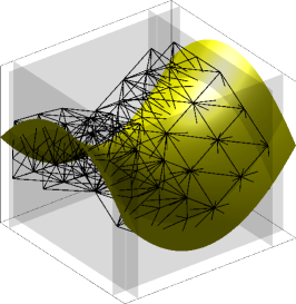
((a)) active background mesh

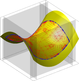
((b)) integration points

((c)) displacements

Fig. 8: (a) Active background mesh, which consists only of cut elements, (b) automatically generated integration points in the domain (red) and on the boundaries (blue), (c) deformed zero-isosurface with scaled displacements $\mathchoice{\displaystyle\bm{u}}{\textstyle\bm{u}}{\scriptstyle\bm{u}}{\scriptscriptstyle\bm{u}}$ by a factor of $2\text{\times}{10}^{3}\text{\,}$.

In the convergence studies, the vertical displacement at $\mathchoice{\displaystyle\bm{x}}{\textstyle\bm{x}}{\scriptstyle\bm{x}}{\scriptscriptstyle\bm{x}}_{i}$ is compared with the given reference displacement. Due to the moderate complexity of the master level-set function, the numerical solution converges rather fast and the element factor $n$ is only varied between $2\leq n\leq 64$. In Fig. 9(a), the results of the convergence study are presented. In particular, the normalized displacement $\nicefrac{{u_{z,i}}}{{u_{z,i,\text{Ref}}}}$ is plotted as a function of the element size $h\sim\nicefrac{{1}}{{n}}$. The behaviour of the convergence is in agreement with the results shown, e.g., in [2, 38, 52]. In particular, the expected locking behaviour is more pronounced for $p=2$ and decreases significantly for higher orders. In Fig. 9(b), the normalized, estimated condition number of the stiffness matrix is plotted as a function of the element size $h\sim\nicefrac{{1}}{{n}}$. The condition numbers are obtained with the MATLAB function condest. It can be seen that the condition numbers increase with quadratic order as expected for second-order PDEs. The jump between the element orders is well-known in the context of higher-order finite element approaches, see e.g., in [26].

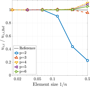
((a)) convergence

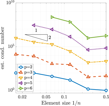
((b)) condition number

Fig. 9: (a) Normalized convergence of reference displacement $u_{z,i,\text{Ref}}=$-9.3355\text{\times}{10}^{-5}\text{\,}$$ at point $\mathchoice{\displaystyle\bm{x}}{\textstyle\bm{x}}{\scriptstyle\bm{x}}{\scriptscriptstyle\bm{x}}_{i}=(0.5,\,0,\,0.25)^{\mathrm{T}}$, (b) normalized condition numbers, the reference value is $1.0797\text{\times}{10}^{10}\text{\,}$, which is the condition number at $n=p=2$.

5.2 Gyroid

The next test case is a partly clamped gyroid and is taken from [28]. The problem is defined in Fig. 10. Similar as above, the yellow surface is the zero-isosurface of the master level-set function $\phi$, the grey planes are the zero-isosurfaces of the slave level-set functions $\psi_{j},\ j\in[1,6]$, which bound the master leve-set function. The blue curve is the clamped edge of the shell.

In contrast to [28], a factor $\pi$ is inserted into the arguments of the trigonometric functions of the master level-set function, which is given in [28, Eq. 43]. Otherwise, the obtained geometry is not in agreement with the presented geometry in [28, Fig. 12]. In addition, the load is decreased by one order of magnitude in order to decrease the deformations, which shall be significantly smaller than the dimensions of the shell. Therefore, the given reference displacement needs to be scaled accordingly to $0.18812$. However, in [28], a different shell model (seven-parameter shell model) is used. Herein, the classical Reissner–Mindlin shell, which is often labelled as five-parameter model, is used and, therefore, we can expect small differences in the displacements. For the Reissner–Mindlin shell model the converged reference displacement is $0.182661$, which is a relative error of $2.9\%$ compared to the seven-parameter model, which can be explained with the differences in the kinematic assumptions between the two shell models. This discrepancy could be decreased with a suitable shear correction factor.

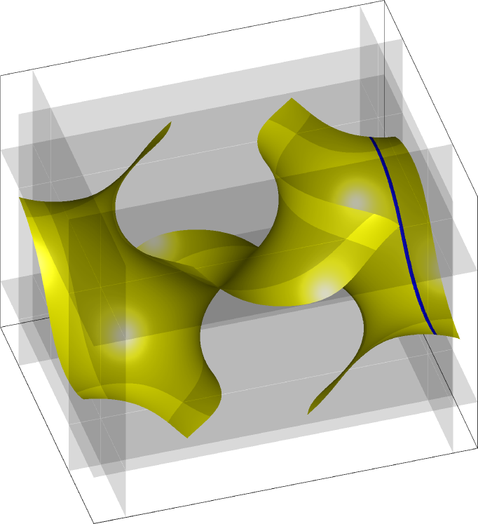
Fig. 10: Definition of the partly clamped gyroid problem.

Analogously to the example above, in Fig. 11, the active background mesh for $p=4$ and the corresponding integration points are shown, where the domain integrations points are plotted in red and the integration points on the boundaries are blue. The deformed zero-isosurface of the shell is plotted in a similar manner as in the first example in Fig. 12(a), where the colors on the surface are the Euclidean norm of the displacement field $\mathchoice{\displaystyle\bm{u}}{\textstyle\bm{u}}{\scriptstyle\bm{u}}{\scriptscriptstyle\bm{u}}^{h}$ and the grey surface indicates the undeformed zero-isosurface.

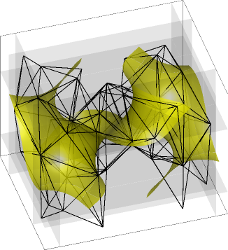
((a)) active background mesh

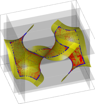
((b)) integration points

Fig. 11: (a) Active background mesh, which consists only of cut elements, (b) automatically generated integration points in the domain (red) and on the boundaries (blue).

In the convergence study, the parameter $n$ is varied between $8\leq n\leq 128$. The coarser levels $n=\{2,4\}$ are skipped due to the more complex shape of the shell. In Fig. 12(b), the results of the convergence analyses are presented. Similar to the first test case, the normalized displacement $\nicefrac{{u_{z,i}}}{{u_{z,i,\text{Ref}}}}$ is plotted as a function of the element size $h\sim\nicefrac{{1}}{{n}}$. For the lower orders $p=\{2,3\}$ the expected locking phenomena is more pronounced compared to the example before. Nevertheless, it is clearly seen that the accuracy for higher orders increases significantly and the behaviour of convergence is in agreement with the results shown, e.g., in [28]. The condition numbers for this example behave in a similar manner as in Fig. 9(b) and, therefore, the plot is omitted for the sake of brevity.

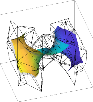
((a)) displacements

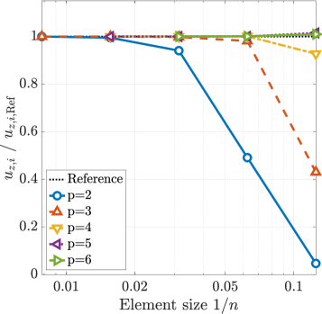
((b)) convergence

Fig. 12: (a) Deformed zero-isosurface, (b) normalized convergence of reference displacement $u_{z,i,\text{Ref}}=0.182661$ at point $\mathchoice{\displaystyle\bm{x}}{\textstyle\bm{x}}{\scriptstyle\bm{x}}{\scriptscriptstyle\bm{x}}_{i}=(2,\,0.5,\,-0.25)^{\mathrm{T}}$.

5.3 Flower-shaped shell

The geometry of the last example is inspired from [52]. The problem is defined in Fig. 13. Analogously as above, the yellow surface is the zero-isosurface of the master level-set function $\phi$ and the intersection with the slave level-set function $\psi$ (grey surface) defines the boundaries of the shell.

A characteristic feature of this test case is that smooth solutions in all involved fields can be expected and, therefore, optimal higher-order convergences rates are enabled. In contrast to the examples before, a reference displacement is not available for the particular example. For the error measurement we employ the concept of residual errors in a similar manner as shown in [23, 51, 52]. The residual errors are the evaluation of the equilibrium in strong form, see Section 3.1, integrated over the domain.

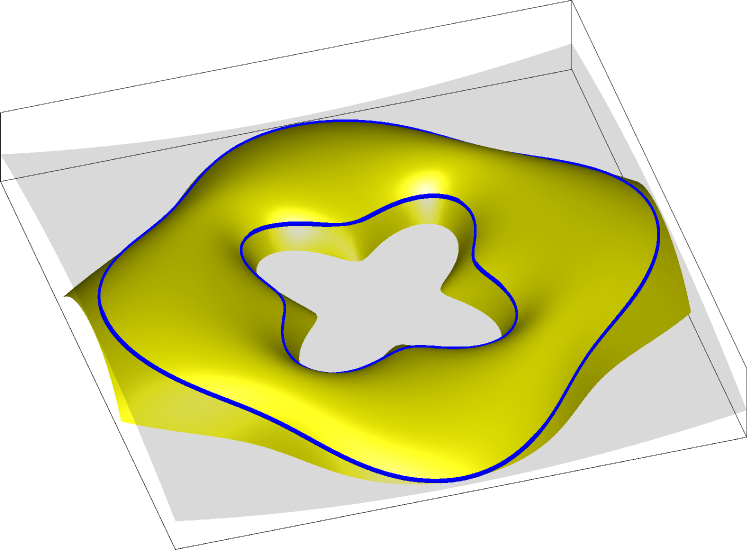
Fig. 13: Definition of shallow flower-shaped shell problem

In particular, the element-wise $L_{2}$-errors of the force and moment equilibrium are computed in the convergence analyses

$$\varepsilon_{\text{rel,residual,F}}^{2} ={{\sum}}_{T=1}^{\tau_{\Omega,h}^{\Gamma}}\ \dfrac{\int_{T}\left[\text{div}_{\Gamma}\mathchoice{\displaystyle\mathbf{n}}{\textstyle\mathbf{n}}{\scriptstyle\mathbf{n}}{\scriptscriptstyle\mathbf{n}}^{\text{real}}_{\Gamma}+\mathchoice{\displaystyle\mathbf{Q}}{\textstyle\mathbf{Q}}{\scriptstyle\mathbf{Q}}{\scriptscriptstyle\mathbf{Q}}\cdot\text{div}_{\Gamma}\mathchoice{\displaystyle\mathbf{q}}{\textstyle\mathbf{q}}{\scriptstyle\mathbf{q}}{\scriptscriptstyle\mathbf{q}}_{\Gamma}+\mathchoice{\displaystyle\mathbf{H}}{\textstyle\mathbf{H}}{\scriptstyle\mathbf{H}}{\scriptscriptstyle\mathbf{H}}\cdot(\mathchoice{\displaystyle\mathbf{q}}{\textstyle\mathbf{q}}{\scriptstyle\mathbf{q}}{\scriptscriptstyle\mathbf{q}}_{\Gamma}\cdot\mathchoice{\displaystyle\bm{n}}{\textstyle\bm{n}}{\scriptstyle\bm{n}}{\scriptscriptstyle\bm{n}}_{\Gamma})+\mathchoice{\displaystyle\bm{f}}{\textstyle\bm{f}}{\scriptstyle\bm{f}}{\scriptscriptstyle\bm{f}}\right]^{2}\ \mathrm{d}A}{\int_{T}\mathchoice{\displaystyle\bm{f}}{\textstyle\bm{f}}{\scriptstyle\bm{f}}{\scriptscriptstyle\bm{f}}^{2}\ \mathrm{d}A}\ ,$$ (5.1)

$$\varepsilon_{\text{residual,M}}^{2} ={{\sum}}_{T=1}^{\tau_{\Omega,h}^{\Gamma}}\ \int_{T}\left[\mathchoice{\displaystyle\mathbf{P}}{\textstyle\mathbf{P}}{\scriptstyle\mathbf{P}}{\scriptscriptstyle\mathbf{P}}\cdot\text{div}_{\Gamma}\mathchoice{\displaystyle\mathbf{m}}{\textstyle\mathbf{m}}{\scriptstyle\mathbf{m}}{\scriptscriptstyle\mathbf{m}}_{\Gamma}-\mathchoice{\displaystyle\mathbf{q}}{\textstyle\mathbf{q}}{\scriptstyle\mathbf{q}}{\scriptscriptstyle\mathbf{q}}_{\Gamma}\cdot\mathchoice{\displaystyle\bm{n}}{\textstyle\bm{n}}{\scriptstyle\bm{n}}{\scriptscriptstyle\bm{n}}_{\Gamma}+\mathchoice{\displaystyle\bm{c}}{\textstyle\bm{c}}{\scriptstyle\bm{c}}{\scriptscriptstyle\bm{c}}\right]^{2}\ \mathrm{d}A\ .$$ (5.2)

For the computation of the residual errors, second-order surfaces derivatives are required which implies a theoretical optimal order of convergence $\mathcal{O}(p-1)$. The numerical solution of the problem is visualized in Fig. 14(b) for $p=4$. The displacements are scaled by a factor of $5\text{\times}{10}^{2}\text{\,}$. The colors on the deformed zero-isosurface are the Euclidean norm of the displacement field $\mathchoice{\displaystyle\bm{u}}{\textstyle\bm{u}}{\scriptstyle\bm{u}}{\scriptscriptstyle\bm{u}}^{h}$. The corresponding integration points are shown in Fig. 14(a) in the same style than before.

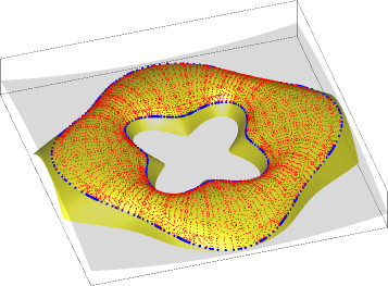
((a)) integration points

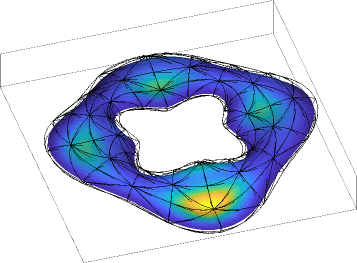
((b)) displacements

Fig. 14: (a) Automatically generated integration points in the domain (red) and on the boundaries (blue), (b) deformed zero-isosurface with scaled displacements $\mathchoice{\displaystyle\bm{u}}{\textstyle\bm{u}}{\scriptstyle\bm{u}}{\scriptscriptstyle\bm{u}}$ by a factor of $5\text{\times}{10}^{2}\text{\,}$.

In the convergence analyses the parameter $n$ is varied between $2\leq n\leq 64$. The results are plotted in Fig. 15. It is noticeable that the pre-asymptotic range is more pronounced for the lower ansatz orders $p=\{2,3\}$. Nevertheless, it is clear that higher-order convergence rates are achieved in both residual errors of Eqs. 5.1 and 5.2. In comparison to the original test case for the Reissner–Mindlin shell presented in [52], the behaviour of convergence in the residual errors obtained here with the Trace FEM are in very good agreement to the results in [52] obtained with isogeometric analysis. Note that the residual error of the moment equilibrium is the absolute, element-wise $L^{2}$-norm, due to $\mathchoice{\displaystyle\bm{c}}{\textstyle\bm{c}}{\scriptstyle\bm{c}}{\scriptscriptstyle\bm{c}}=\mathchoice{\displaystyle\bm{0}}{\textstyle\bm{0}}{\scriptstyle\bm{0}}{\scriptscriptstyle\bm{0}}$. When comparing $\varepsilon_{\text{residual,M}}$ in Fig. 15(b) with results obtained by the authors in [52], the difference in the magnitudes is traced back to the material parameters and a modified geometry.

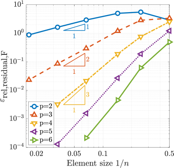
((a)) force equilibrium

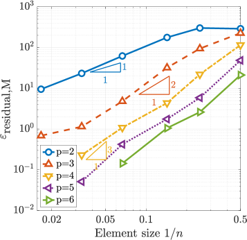
((b)) moment equilibrium

Fig. 15: (a) Residual error of the force equilibrium $\varepsilon_{\text{rel,residual,F}}$, (b) residual error of the moment equilibrium $\varepsilon_{\text{residual,M}}$.

6 Conclusions

A higher-order accurate Trace FEM approach for implicitly defined shells is presented. The shell geometry is implicitly defined by means of multiple level-set functions. Due to the implicit geometry definition, a parametrization of the midsurface is not available and the classical shell formulations of the linear Reissner–Mindlin shell are not applicable. Therefore, a more general shell formulation in the frame of the TDC, which extends also to implicitly defined shells, is employed.

The Trace FEM is a fictitious domain method for PDEs on manifolds enabling higher-order accuracy when the following three aspects (well-known for general FDMs) are addressed properly: (i) numerical integration, (ii) stabilization and (iii) enforcement of essential boundary conditions. Each aspect is carefully detailed herein, thus proposing an optimal higher-order accurate FDM for shells for the first time. The employed integration technique extends to multiple level-set functions and is based on a recursive reconstruction of the cut reference element into higher-order integration cells. The normal derivative volume stabilization also extends to higher-order shape functions without additional measures and the choice of the stabilization parameter is rather flexible. The essential boundary conditions are enforced with the non-symmetric version of Nitsche’s method which is a consistent approach and does neither require additional stabilization terms nor the discretization of auxiliary fields. In addition, the tangentiality constraint on the difference vector is automatically built-in with an additional projection of a full 3D vector combined with a consistent stabilization term. In the numerical results, classical and new benchmark examples are presented and optimal higher-order convergence rates are achieved when the physical fields are sufficiently smooth.

References

- [1] Başar, Y.; Krätzig, W.B.: Mechanik der Flächentragwerke. ViewegTeubner Verlag, Braunschweig, 1985.
- [2] Bathe, K.J.; Iosilevich, A.; Chapelle, D.: An evaluation of the MITC shell elements. Computers & Structures, 75, 1–30, 2000.
- [3] Bischoff, M.; Ramm, E.; Irslinger, J.: Models and Finite Elements for Thin-Walled Structures. In Encyclopedia of Computational Mechanics (Second Edition). (Stein, E.; Borst, R.; Hughes, T. J.; Hughes, T. J., Eds.), John Wiley & Sons, 2017.
- [4] Blaauwendraad, J.; Hoefakker, J.H.: Structural Shell Analysis, Vol. 200, Solid Mechanics and Its Applications. Springer, Berlin, 2014.
- [5] Bonito, A.; Demlow, A.; Nochetto, R.H.: Chapter 1 - Finite Element Methods for the Laplace-Beltrami Operator. In Geometric Partial Differential Equations - Part I. (Bonito, A.; Nochetto, R.H., Eds.), Vol. 21, Handbook of Numerical Analysis, Elsevier, Amsterdam, 1–103, 2020.
- [6] Brandner, P.; Reusken, A.: Finite element error analysis of surface Stokes equations in stream function formulation. arXiv e-prints, 2019. arXiv: 1910.09221.
- [7] Burman, E.: A penalty-free nonsymmetric Nitsche-type method for the weak imposition of boundary conditions. SIAM J. Numer. Anal., 50, 1959–1981, 2012.
- [8] Burman, E.; Claus, S.; Hansbo, P.; Larson, M.G.; Massing, A.: CutFEM: Discretizing geometry and partial differential equations. Internat. J. Numer. Methods Engrg., 104, 472–501, 2015.
- [9] Burman, E.; Elfverson, D.; Hansbo, P.; Larson, M.G.; Larsson, K.: Shape optimization using the cut finite element method. Comp. Methods Appl. Mech. Engrg., 328, 242–261, 2018.
- [10] Burman, E.; Hansbo, P.; Larson, M.G.: A stabilized cut finite element method for partial differential equations on surfaces: The Laplace-Beltrami operator. Comp. Methods Appl. Mech. Engrg., 188–207, 2015.
- [11] Burman, E.; Hansbo, P.; Larson, M.G.; Massing, A.: Cut finite element methods for partial differential equations on embedded manifolds of arbitrary codimensions. ESAIM: Mathematical Modelling and Numerical Analysis, 52, 2247–2282, 2018.
- [12] Calladine, C. R.: Theory of Shell Structures. Cambridge University Press, Cambridge, 1983.
- [13] Cenanovic, M.; Hansbo, P.; Larson, M.G.: Cut finite element modeling of linear membranes. Comp. Methods Appl. Mech. Engrg., 310, 98–111, 2016.
- [14] Chapelle, D.; Bathe, K.J.: Fundamental considerations for the finite element analysis of shell structures. Computers & Structures, 66, 19–36, 1998.
- [15] Chapelle, D.; Bathe, K.J.: The mathematical shell model underlying general shell elements. Internat. J. Numer. Methods Engrg., 48, 289–313, 2000.
- [16] Delfour, M.C.; Zolésio, J.P.: A Boundary Differential Equation for Thin Shells. J. Differential Equations, 119, 426–449, 1995.
- [17] Delfour, M.C.; Zolésio, J.P.: Tangential Differential Equations for Dynamical Thin Shallow Shells. J. Differential Equations, 128, 125–167, 1996.
- [18] Delfour, M.C.; Zolésio, J.P.: Shapes and Geometries: Metrics, Analysis, Differential Calculus, and Optimization. SIAM, Philadelphia, 2011.
- [19] Demlow, A.: Higher-order finite element methods and pointwise error estimates for elliptic problems on surfaces. SIAM J. Numer. Anal., 47, 805–827, 2009.
- [20] Dziuk, G.: Finite Elements for the Beltrami operator on arbitrary surfaces, 142–155. Springer, Berlin, 1988.
- [21] Dziuk, G.; Elliott, C.M.: Finite element methods for surface PDEs. Acta Numerica, 22, 289–396, 2013.
- [22] Farshad, M.: Design and Analysis of Shell Structures. Springer, Berlin, 1992.
- [23] Fries, T.P.: Higher-order surface FEM for incompressible Navier-Stokes flows on manifolds. Int. J. Numer. Methods Fluids, 88, 55–78, 2018.
- [24] Fries, T.P.; Omerović, S.: Higher-order accurate integration of implicit geometries. Internat. J. Numer. Methods Engrg., 106, 323–371, 2016.
- [25] Fries, T.P.; Omerović, S.; Schöllhammer, D.; Steidl, J.: Higher-order meshing of implicit geometries - Part I: Integration and interpolation in cut elements. Comp. Methods Appl. Mech. Engrg., 313, 759–784, 2017.
- [26] Fries, T.P.; Schöllhammer, D.: Higher-order meshing of implicit geometries - Part II: Approximations on manifolds. Comp. Methods Appl. Mech. Engrg., 326, 270–297, 2017.
- [27] Fries, T.P.; Schöllhammer, D.: A unified finite strain theory for membranes and ropes. Comp. Methods Appl. Mech. Engrg., 365, 113031, 2020.
- [28] Gfrerer, M.H.; Schanz, M.: High order exact geometry finite elements for seven-parameter shells with parametric and implicit reference surfaces. Comput. Mech., 64, 133–145, 2019.
- [29] Grande, J.; Lehrenfeld, C.; Reusken, A.: Analysis of a high-order trace finite element method for PDEs on level set surfaces. SIAM J. Numer. Anal., 56, 228–255, 2018.
- [30] Grande, J.; Reusken, A.: A higher order finite element method for partial differential equations on surfaces. SIAM, 54, 388–414, 2016.
- [31] Gross, S.; Jankuhn, T.; Olshanskii, M.A.; Reusken, A.: A trace finite element method for vector-laplacians on surfaces. SIAM J. Numer. Anal., 56, 2406–2429, 2018.
- [32] Guo, Y.; Do, H.; Ruess, M.: Isogeometric stability analysis of thin shells: From simple geometries to engineering models. Internat. J. Numer. Methods Engrg., 118, 433–458, 2019.
- [33] Hansbo, P.; Larson, M.G.: Finite element modeling of a linear membrane shell problem using tangential differential calculus. Comp. Methods Appl. Mech. Engrg., 270, 1–14, 2014.
- [34] Hansbo, P.; Larson, M.G.; Larsson, F.: Tangential differential calculus and the finite element modeling of a large deformation elastic membrane problem. Comput. Mech., 56, 87–95, 2015.
- [35] Jankuhn, T.; ; Reusken, A.: Higher Order Trace Finite Element Methods for the Surface Stokes Equations. arXiv e-prints, 2019. arXiv: 1909.08327.
- [36] Jankuhn, T.; Olshanskii, M.A.; Reusken, A.: Incompressible Fluid Problems on Embedded Surfaces Modeling and Variational and Formulations. Interfaces Free Bound., 20, 353–377, 2018.
- [37] Jankuhn, T.; Olshanskii, M.A.; Reusken, A.; Zhiliako, A.: Error Analysis of Higher Order Trace Finite Element Methods for the Surface Stokes Equations. arXiv e-prints, 2020. arXiv: 2003.06972.
- [38] Kiendl, J.; Marino, E.; De Lorenzis, L.: Isogeometric collocation for the Reissner-Mindlin shell problem. Comp. Methods Appl. Mech. Engrg., 325, 645–665, 2017.
- [39] Larson, M.G.; Zahedi, S.: Stabilization of high order cut finite element methods on surfaces. IMA J. Numer. Anal., 40, 1702–1745, 2020.
- [40] Lehrenfeld, C.: High order unfitted finite element methods on level set domains using isoparametric mappings. Comp. Methods Appl. Mech. Engrg., 300, 716–733, 2016.
- [41] Lehrenfeld, C.; Olshanskii, M.A.; Xu, X.: A stabilized trace finite element method for partial differential equations on evolving surfaces. SIAM, 56, 1643–1672, 2018.
- [42] Müller, B.; Kummer, F.; Oberlack, M.: Highly accurate surface and volume integration on implicit domains by means of moment-fitting. Internat. J. Numer. Methods Engrg., 96, 512–528, 2013.
- [43] Olshanskii, M.A.; Quaini, A.; Reusken, A.; Yushutin, V.: A finite element method for the surface Stokes problem. SIAM J. Sci. Comput., 40, A2492–A2518, 2018.
- [44] Olshanskii, M.A.; Reusken, A.: A finite element method for surface PDEs: Matrix properties. Numer. Math., 114, 491–520, 2009.
- [45] Olshanskii, M.A.; Reusken, A.: Trace finite element methods for PDEs on surfaces. Lecture Notes in Computational Science and Engineering, 121, 211–258, 2017.
- [46] Olshanskii, M.A.; Reusken, A.; Grande, J.: A finite element method for elliptic equations on surfaces. SIAM, 47, 3339–3358, 2009.
- [47] Olshanskii, M.A.; Xu, X.: A trace finite element method for PDEs on evolving surfaces. SIAM, 39, A1301–A1319, 2017.
- [48] Osher, S.; Fedkiw, R.P.: Level Set Methods and Dynamic Implicit Surfaces. Springer, Berlin, 2003.
- [49] Reusken, A.: Analysis of trace finite element methods for surface partial differential equations. IMA J. Numer. Anal., 35, 1568–1590, 2014.
- [50] Schillinger, D.; Harari, I.; Hsu, M.C.; Kamensky, D.; Stoter, S.K.F.; Yu, Y.; Zhao, Y.: The non-symmetric Nitsche method for the parameter-free imposition of weak boundary and coupling conditions in immersed finite elements. Comp. Methods Appl. Mech. Engrg., 309, 625–652, 2016.
- [51] Schöllhammer, D.; Fries, T.P.: Kirchhoff-Love shell theory based on tangential differential calculus. Comput. Mech., 64, 113–131, 2019.
- [52] Schöllhammer, D.; Fries, T.P.: Reissner–Mindlin shell theory based on tangential differential calculus. Comp. Methods Appl. Mech. Engrg., 352, 172–188, 2019.
- [53] Schöllhammer, D.; Fries, T.P.: Reissner–Mindlin shell theory based on Tangential Differential Calculus. John Wiley & Sons, Chichester, 2019, PAMM.
- [54] Schöllhammer, D.; Fries, T.P.: A unified approach for shell analysis on explicitly and implicitly defined surfaces. Form and Force: Proceedings of the IASS Symposium 2019 - Structural Membranes 2019, C. Lázaro, K.U. Bletzinger, E. Oñate (eds.), Barcelona, 750–757, 2019, Form and Force: Proceedings of the IASS Symposium 2019 - Structural Membranes 2019, C. Lázaro, K.U. Bletzinger, E. Oñate (eds.).
- [55] Sethian, J.A.: Level Set Methods and Fast Marching Methods. Cambridge University Press, Cambridge, 2nd edition, 1999.
- [56] Simo, J.C.; Fox, D.D.: On a stress resultant geometrically exact shell model. Part I: Formulation and optimal parametrization. Comp. Methods Appl. Mech. Engrg., 72, 267–304, 1989.
- [57] Simo, J.C.; Fox, D.D.; Rifai, M.S.: On a stress resultant geometrically exact shell model. Part II: The linear theory; Computational aspects. Comp. Methods Appl. Mech. Engrg., 73, 53–92, 1989.
- [58] Wempner, G.; Talaslidis, D.: Mechanics of Solids and Shells: Theories and Approximations. CRC Press LLC, Florida, 2002.
- [59] Zingoni, A.: Shell Structures in Civil and Mechanical Engineering: Theory and analysis. ICE Publishing, London, 2nd edition, 2018.