Type IIP Supernova Progenitors III: Blue to Red Supergiant Ratio in Low Metallicity Models with Convective Overshoot

Abstract

The distribution of stars in the Hertzsprung Russell diagram (HRD) for a stellar conglomeration represents a snapshot of its evolving stellar population. Some of the supergiant stars may transit the HRD from blue to red and then again to blue during their late evolutionary stages, as exemplified by the progenitor of SN 1987A. Others may transit a given part of the HRD more than twice in a “blue loop” and end up as red supergiants before they explode. Since stars in blue loops spend a considerable part of their lives there, these stages may change the relative number of modeled supergiants in the HRD. Their lifetimes in turn depend upon the initial mass of the star, how convection in its interior is modeled, and how much mass loss takes place during its evolution. The observed ratio of the number of blue to red supergiants and yellow to red supergiants sensitively test the stellar evolution theory. We compare modeled number ratios of these supergiants with observed data from the Large Magellanic Cloud as it has a metallicity very similar to that of the environment of SN 2013ej. We successfully model these by taking into account moderate (exponential) convective overshooting. We explore its effect on the final radius and mass of the star prior to core collapse. The radius differs dramatically with overshoot. These factors controlling pre-supernova structure may affect the post-explosion optical/IR light curves and spectral development.

1 Introduction

Massive stars transit red-ward on the Hertzsprung Russell diagram (HRD) from a blue supergiant (BSG) phase after they have fully exhausted hydrogen in their core. The BSG (B0 to A9 spectral types) progenitor enters the red supergiant (RSG - K0 to M3 I type) phase after passing through a yellow supergiant (YSG - F0 to G9 I) phase. Some of the RSGs may evolve back towards blue at an intermediate stage of their lives, passing through the YSG phase for a second time. These stars at the BSG phase after it has already been a RSG may collapse to give rise to a supernova like SN 1987A (Arnett et al., 1989). Other stars, after traversing a part of their blue-ward track, may turn back and end up in the RSG stage before they collapse to give rise to the more canonical type IIP or IIL supernovae. Many of these RSGs retain a lot of hydrogen envelope at the time of collapse. This doubling-back of the track of the supergiants in the HRD is known as the blue loop. Stars having blue loops spend a significant part of their lifetimes during core helium burning in the blue part of the HRD. The existence of blue loops in the evolutionary tracks may change the number distribution of different types of supergiants in the HRD.

The distribution of stars in the HRD of a system like the LMC, where all stars are at approximately the same distance from us gives us a snapshot of the stellar conglomeration in transition over its very long life. The number of stars in a given region while they are in transit from one part of the HRD to another in a steady state is proportional to the lifetime of that given phase in the HRD. Thus, this distribution reveals how massive stars are actually evolving over time. For a comparison between the models and the observed data, we need to know how many stars are in the system for a given mass range (the initial mass function), since stellar lifetimes are known to vary strongly with the initial mass of the stars. Another important aspect of the stellar lifetimes is how convection goes on in the stellar interior, both in the nuclear fuel burning core regions, as well as, in the convective envelope which forms the star’s outer regions. The stellar evolution code MESA models the extra mixing of elements beyond the convective boundary by ”convective overshooting”, which is parameterized in terms of a scale factor $f$ that operates on the local pressure scale height. The luminosity of the star at any given time is not only controlled by its initial mass but also by the extent of the convective overshoot.

The intermediate stage YSGs are relatively rare (see Drout et al., 2009; Neugent et al., 2012b, 2010). A sample of these supergiants that is complete can provide a “magnifying glass” (Kippenhahn & Weigert, 1990) for tests of stellar evolution theory in a particular environment. Moreover, as Neugent et al. (2010) point out, it is vital to have reliable evolutionary tracks of the luminous stars to interpret the spectra of distant galaxies using population synthesis codes as often the individual stars cannot be resolved in these galaxies. Stellar evolutionary models are also necessary to study mixed age populations of stars and their initial mass functions.

Computing the ratio of numbers of blue to red supergiants (B/R) and of yellow to red supergiants (Y/R) to match the data in varying galactic environments is thus one of the most challenging problems in astrophysics. The B/R ratio has been observed to be a steeply rising function of metallicity, Z in an ensemble of massive stars in galaxies or a set of young clusters (see Langer & Maeder, 1995, and references therein). However, most of the model calculations fail to fit the ratio for a given set of parameters as a function of metallicity. The ratio is sensitive to mass loss, convection and other mixing processes. Since convective overshoot is an important ingredient of mixing in both the nuclear burning core or its edge as well as in the stellar envelope surrounding it, the B/R ratio may be an important diagnostic of the extent of convective overshoot as well. In this paper, we explore the effects of convective overshoot on the B/R ratio in the case of low metallicity models (Z = 0.006). In our companion Paper I (Wagle et al., 2019), we have discussed how the convective overshoot affects the evolution of a 13 M_☉ star (with Z = 0.006) in terms of its internal structure as well as the evolution in the HRD, especially the existence of blue loop. Here, we extend the methods to a range of stellar masses (12–15 M_☉) to study the effects of convective overshoot on the predicted B/R ratio. We then compare our predicted values to the observed ratio for the Large Magellanic Cloud (LMC), which has similar metallicity value (Z = 0.007) and sufficient recent observational data to make this comparison viable.

In section 2, we review the literature for the observed B/R ratio as a function of metallicty in the LMC and other galaxies. In section 3 we review the selection of observed LMC supergiants for comparing a subset of the data from Neugent et al. (2012b) with our model evolutionary calculations. In section 4, we discuss the computational methods for stellar evolution models using the code Modules for Experiments in Stellar Astrophysics (MESA, Paxton et al., 2011, 2013, 2015, 2018). In section 5, we describe the calculations of predicted B/R and Y/R ratios using the models discussed in the previous section. In addition, we discuss the observed B/R and Y/R ratios for the LMC to compare with the predicted ratios. We also discuss the variation of the final radius and mass of the pre-supernova star with overshoot factor. In section 6, we mention how these variations may affect the post-explosion supernova light curves and spectra along with our conclusions.

2 B/R Ratio and Its Dependence on Metallicity

The ratio of B/R supergiants is known to be particularly sensitive to the metallicity of the environment where the supergiant stars reside. The ratio and its Z-dependence obtained from a number of clusters in the Milky Way galaxy and the Magellanic Clouds have been re-examined by Eggenberger et al. (2002). They give a normalized relation of the B/R (to the solar neighborhood value) in terms of metallicity as:

$${(B/R)/(B/R)_{\odot}}\sim 0.05\times e^{{3Z/Z_{\odot}}}$$ (1)

Eggenberger et al. (2002) find that the ratio at solar metallicity $(B/R)_{\odot}=$ 3 when including O, B and A supergiants in blue for log age interval of 6.8–7.5. They chose stars in stellar clusters instead of field stars as the stars in the clusters have same distance, age and chemical composition. They identified the supergiants based on spectroscopic measurements instead of photometric colors to accurately differentiate supergiants and main sequence stars. They showed that the B/R ratio remains more or less the same even if different log age intervals are chosen. They however do not give a value for B/R ratio of the LMC due to lack of sufficient spectroscopic data for the young clusters in the LMC. If we consider the relation given above in equation 1, then B/R ratio for the LMC would be around 0.4, assuming a ratio 3.6 for solar neighborhood (counting only the B-type stars). Eggenberger et al. (2002) also tabulate the ratio for the photometric count with limiting visual magnitude ($M_{vlim}$) in their table 3. This value varies from 2.5 at $M_{vlim}=-$3.25 to 5.7 at $M_{vlim}=-$2.0 for the LMC. Langer & Maeder (1995) note that the observed B/R ratio in literature is found to be around 0.6 when strictly B and red supergiants are counted for the young cluster NGC 330 in the SMC. However, this value is based on the observations of a single star cluster. They found the same ratio to be 3.6 for young clusters in the solar neighborhood. Humphreys & McElroy (1984) get the ratio of B/R of 10 for the LMC & 28 for the solar neighborhood, if all O, B and A stars are included in blue. However, these blue counts include main-sequence stars as well. Langer & Maeder (1995) give B/R ratio of 10 for stars and associations in the LMC for limiting bolometric magnitude, $M_{bol}=-$7.5. However, as mentioned earlier these blue counts include main sequence stars.

Humphreys & Davidson (1979) note that the B/R ratio determined as a function of luminosity decreases with decreasing luminosity. They also find that the B/R ratio changes less strongly with galactocentric distance (and hence, metallicity) if the ratio is restricted to less luminous supergiants $M_{bol}\geq-$8.5.

The calculated B/R ratio is extremely sensitive to model parameters like metallicity, mass loss, convection and other mixing processes (see Maeder & Meynet, 2001; Langer & Maeder, 1995). For a given set of input parameters, the computational models have trouble predicting the B/R ratio for both the high and the low end of the metallicities, simultaneously. There are more number of RSG in the SMC (Z = 0.002) than the models have previously predicted. Langer & Maeder (1995) have reviewed previous work that test the B/R ratios in different environments. The models that do not use overshooting or semiconvection could realize acceptable agreement for the solar neighborhood but failed to produce the relative number of observed red supergiants at low Z (e.g. Brunish et al., 1986; Brunish & Truran, 1982b, a). Stothers & Chin (1992) addressed this problem and showed that use of Ledoux criterion reproduce well the observed B/R ratio at low Z environment of the SMC, but not for Z $>$ 0.006 (e.g. for the LMC and the solar neighborhood). Further, models by Arnett (1991) that use Ledoux criterion and semiconvection fit well the distribution of supergiants in the LMC as given in Fitzpatrick & Garmany (1990). Langer & Maeder (1995) summarize that the models with Schwarzschild’s criterion (with or without convective overshoot mixing) are favorable for solar metallicity environments, while models using the Ledoux criterion with presence of overshooting at the core as well as the base of hydrogen envelope, and including semiconvection yield better results at low Z.

3 Selection of the Observed LMC Supergiants for Model Comparison

Table 1: The observed LMC supergiants and selection criteria

Selection	Observed Numbers in the data for
Criteria	BSG	YSG	RSG	Total Supergiants
Neugent et al. (2012b)	———— 1528 ————		865	2393
Associated Vizier Catalog	———— 1447 ————		521	1968
Category 1	————0309 ————		506	0815
Effective Temperature	($log_{10}(T_{eff}/\rm K)$$>$ 3.875)	(3.875 $\geq$ $log_{10}(T_{eff}/\rm K)$$>$ 3.68)	(3.68 $\geq$ $log_{10}(T_{eff}/\rm K)$)
	163	109	543	0815
Effective Temperature	(4.0 $\geq$ $log_{10}(T_{eff}/\rm K)$$>$ 3.875)	(3.875 $\geq$ $log_{10}(T_{eff}/\rm K)$$>$ 3.68)	(3.68 $\geq$ $log_{10}(T_{eff}/\rm K)$)
	112	109	543	0764
4.0 $<$ $log_{10}(L/L_{\odot})$$<$ 5.0	097	087	514	0698
4.2 $<$ $log_{10}(L/L_{\odot})$$<$ 5.0	097	087	430	0614

Note. — The LMC supergiants observed by Neugent et al. (2012b) are listed in this table along with various criteria used to limit the observation sample in order to make comparison with the model calculations of the B/R and Y/R ratios. Neugent et al. initially observed 2393 supergiants (first row), however, they found nothing but sky for 69 YSGs and 343 RSG candidates. Most of these missing RSG candidates are hypothesized to be dust-enshrouded objects. The associated Vizier Catalog (Neugent et al., 2012a) contains candidates excluding those that yielded nothing but the sky in spectroscopic observations. Category 1 label is used to identify the LMC membership. We re-distribute the observed category 1 stars in the BSG, YSG and RSG categories using the effective temperature criteria. A more restrictive $T_{eff}$$\leq$ 10,000 K criteria is used for BSG candidates, as Neugent et al. claim that their data is complete up to $T_{eff}$$\approx$ 10,000 K. The luminosity limits are applied to select candidates for comparison with the models. The numbers in the last row are used for comparison with the model calculations.

There are many surveys of the LMC supergiants available in the literature. However, most of the observational studies focus on the red and blue supergiant populations, separately. For example, Davies et al. (2018) lists 225 previously observed RSGs+YSGs in the LMC, out of which 200 RSGs have determined spectral types. On the other hand, Fitzpatrick & Garmany (1990) only consider the LMC stars with spectral type between O3 and G7. Urbaneja et al. (2017) also observed spectra of 32 LMC blue supergiants to study gravity-luminosity relationship. Different surveys introduce different methodology of gathering and analyzing the data which may introduce different biases in each survey. It may be difficult to account for these differences and determine the correction factors of incompleteness, etc. Therefore, we need a complete dataset that includes observations of both blue and red supergiant stars observed in the same field(s) or cluster(s) and treats data analysis and census in a homogeneous way to be able to determine the relevant observed B/R and Y/R ratios. The dataset published by Neugent et al. (2012b) comes closest to this approximation. They observed supergiant stars in the LMC using the Cerro Tololo 4 m telescope and a 138-fiber multi-fiber, multi-object spectrometer Hydra in 64 fields (each of which has a 40 arcmin field of view). They include both RSGs (K and M type supergiants) and YSGs (F and G-type supergiants) as well as some BSG stars (B and A type supergiants).

3.1 Candidate selection for observations by Neugent et al.

Neugent et al. (2012b) identified the LMC YSG and RSG candidates in a multi-step process. They initially selected the YSG and RSG candidates from the US Naval Observatory CCD Astrograph Catalog Part 3 (UCAC3), within a 3.5 degree radius window centered on the LMC’s visible disk and with data on color and magnitude ranges . They used UCAC3 quality codes to eliminate galaxies, clusters and double stars in the field.

Neugent et al. claimed that the following procedure gave a complete sample of the YSGs down to 12 M_☉ . In selecting the color magnitude ranges they used a $T_{eff}$ range of 4800–7500 K for the YSGs and defined a K magnitude limit as a function of J$-$K for a 12 M_☉ star obtained from ATLAS9 atmosphere models (Kurucz, 1992). They, however, defined a flat K-magnitude cutoff at $K_{2MASS}=10.2$ mag when $(J-K)_{2MASS}>0.9$ for the RSGs (see figure 2 of Neugent et al., 2012b). Using these criteria they obtained 2187 YSG candidates and 1949 RSG candidates from the UCAC3 catalog.

Neugent et al. (2012b) could however observe only 1528 YSG candidates and 865 RSG candidates. These observed numbers are a fraction (70% for YSG and 44% for the RSGs) of the larger number of candidates selected from the UCAC3 catalog mentioned above. They discovered that 69 of the YSG candidates and 343 of RSG candidates yielded nothing but sky background when their spectra at these sky coordinates were examined.

The published Vizier catalog consists of 1447 YSG candidates and 521 RSG candidates. This is 95% of the YSGs and 60% of the RSG candidates initially observed by Neugent et al. (2012b).

3.2 LMC Membership

A reliable method for the removal of the foreground (dwarf) star contamination for the supergiant samples in the LMC and other nearby galaxies has been a significant concern for many studies. It is straightforward to separate the extragalactic RSGs from the foreground red dwarfs and giants by a two color diagram (Massey, 1998; Massey et al., 2009). However, this method does not work well for the YSGs (see Drout et al., 2009), since there is little or no separation of tracks in the two-color diagram for late F-type through early K-type supergiants. This is thus more of a problem for the YSGs in the LMC than for the RSGs. Foreground stars contaminating the field that contains the target stars of the LMC were weeded out by excluding those stars with absolute proper-motion values greater than 15 $mas\;yr^{-1}$ in RA or Dec. In fact, Neugent et al. (2012b) successfully identified the RSGs in the LMC using color and proper motion alone. For the YSGs they required the additional criterion of radial velocities to separate these from the galactic foreground stars which have distinctly separate and lower radial velocity distribution. The large systemic radial velocity of the LMC and its clear separation from the velocity distribution of the stars in the Milky Way is a key factor in determining the LMC membership.

The spectroscopic observations to measure the radial velocities of the stars to discriminate their membership of the LMC Taking account of the large radial velocity separation between the LMC and Milky Way stars, they found that 309 YSG candidates and 506 RSG candidates have radial velocities higher than 200 $\rm km\ s^{-1}$ and are probable LMC supergiants (labeled as category 1 stars ). They found 8 candidates, all of which are YSGs, have 155 $\rm km\ s^{-1}$$<v_{rad}<$ 200 $\rm km\ s^{-1}$. They labeled these stars as category 2 (possible but not probable) LMC supergiants. We use the category 1 stars listed in the Vizier catalog giving a total of 815 YSG+RSG candidates .

3.3 Blue, Yellow, and Red Supergiant candidate selection for comparison with our models

The blue/yellow to red ratio of supergiants in the LMC has been debated in the literature over a long time and is critical for comparing with model comparisons. We recapitulate below briefly the multiple filters by which the number of observed supergiants are identified and selected . As already mentioned, Neugent et al. (2012b) combine together B and A type stars with F and G type stars into their broadly defined “YSG” category. When we distinguish stars with $log_{10}(T_{eff}/\rm K)$$>$ 3.875 as BSGs, 3.875 $\geq$ $log_{10}(T_{eff}/\rm K)$$>$ 3.68 as YSGs, $log_{10}(T_{eff}/\rm K)$$<$ 3.68 as RSGs, we get the candidates redistributed in to 163 BSG, 109 YSG, and 543 RSG candidates in these intervals (a total of 815 supergiants). The number of observed BSG, YSG and RSGs arising from various selection criteria relevant to our model calculations are summarized in our Table 1. Since Neugent et al. (2012b) are confident about completeness of the data only upto 4.0 $\geq$$log_{10}(T_{eff}/\rm K)$, we further report the restricted number of the BSG candidates in row 5 of Table 1. Finally, since we are interested in comparing predictions of our model calculations with those of a specific set of mass ranges and overshoot factors, that display the Blue Loops, we report in last two rows of the table the observed number of BSGs, YSGs and RSGs with above temperature ranges in specific luminosity bands, which are discussed in section 5.1.

3.4 Dust Enshrouded RSGs

these RSGs cannot be spurious sources. About 93% of these RSG candidates have both proper motions measured from the UCAC3 and 2MASS photometry. These candidates fall in the region of large J$-$K values (¿ 1.2 mag), i.e they are very cool stars ($T_{eff}$$<$ 3500 K). The authors conjectured that many of these stars showed evidence of being highly dust-enshrouded. Since the Hydra MOS spectroscopic pass band falls in the $I$-band, a typical M0 RSG with $T_{eff}$= 3800 K and $V_{0}=13.5$ and with the normal amount of LMC reddening $E(B-V)=0.13$, can be expected to have $V\sim 14.0$ mag, $K\sim 9.6$ mag and $I\sim 12.0$ mag . However if the star is shrouded in a thick circumstellar dust shell of a normal reddening law, resulting in $J-K=1.8$ mag, with $E(J-K)=0.8$ (and hence $A_{V}=4.9$ mag instead of the normal $A_{V}=0.5$ mag), the star will be 3 mag fainter in the spectral passband $I$ (or at about $I=15$ mag) than the normal stars for which good data is obtained with their exposures. These stars will therefore be at the faintest end of detectability.

Table 2: Model Lifetimes for RSG/YSG/BSG phases

overshoot	$\rm\tau_{B_{1}}$	$\rm\tau_{Y_{1}}$	$\rm\tau_{R_{1}}$	$\rm\tau_{Y_{2}}$	$\rm\tau_{B_{2}}$	$\rm\tau_{Y_{3}}$	$\rm\tau_{R_{2}}$	Total Model Timescale in $\rm 10^{3}$ years				$\rm\tau_{BSG^{*}}/\tau_{RSG}$	$\rm\tau_{BSG}/\rm\tau_{RSG}$	$\rm\tau_{YSG}/\rm\tau_{RSG}$	$\rm log_{10}(L,T_{eff})$
parameter, f	(BSG 1)	(YSG 1)	(RSG 1)	(YSG 2)	(BSG 2)	(YSG 3)	(RSG 2)	BSG∗	BSG	YSG	RSG				at T.P.
12 M☉
0.019	11.64	02.43	0672.51	5.98	652.96	09.31	069.63	041.92	664.60	017.71	0742.15	0.060	0.900	0.020	(4.60, 4.13)
0.020	11.26	02.34	0703.07	6.23	594.41	12.91	70.65	053.99	605.67	021.47	0773.72	0.070	0.780	0.030	(4.60, 4.12)
0.021	10.82	02.29	0813.34	7.24	453.03	17.68	73.24	102.86	463.85	027.21	0886.58	0.120	0.520	0.030	(4.61, 4.05)
0.022	10.42	02.25	0865.63	8.09	367.99	26.56	77.42	265.87	378.42	036.90	0943.06	0.280	0.400	0.040	(4.61, 4.01)
0.023	10.07	02.22	1324.79	–	–	–	–	007.65	010.07	002.22	1324.79	0.006	0.008	0.002	N/A
0.024	09.87	02.15	1304.95	–	–	–	–	007.53	009.87	002.15	1304.95	0.006	0.008	0.002	N/A
0.025	09.52	02.10	1283.30	–	–	–	–	007.24	009.52	002.10	1283.30	0.006	0.007	0.002	N/A
0.030	08.05	01.90	1186.52	–	–	–	–	006.09	008.05	001.90	1186.52	0.005	0.007	0.002	N/A
0.031	07.87	01.87	1171.15	–	–	–	–	005.95	007.87	001.87	1171.15	0.005	0.007	0.002	N/A
0.050	04.74	01.27	0948.84	–	–	–	–	003.54	004.74	001.27	0948.84	0.004	0.005	0.001	N/A
13 M☉
0.015	11.23	02.44	1367.13	–	–	–	–	008.62	011.23	002.44	1367.13	0.006	0.008	0.002	N/A
0.017	10.37	02.20	1321.51	–	–	–	–	008.01	010.37	002.20	1321.51	0.006	0.008	0.002	N/A
0.018	10.03	02.14	0642.59	4.55	536.94	20.58	85.95	066.87	546.97	027.26	0728.54	0.090	0.750	0.040	(4.67, 4.08)
0.020	09.40	01.98	0351.03	3.96	816.07	05.64	53.22	022.91	825.47	011.58	0404.25	0.060	2.040	0.030	(4.69, 4.14)
0.025	07.84	01.75	0431.04	4.18	648.10	08.18	46.16	031.80	655.94	014.11	0477.21	0.070	1.370	0.030	(4.72, 4.13)
0.030	06.85	01.57	0542.97	6.03	429.05	20.19	58.16	084.69	435.90	027.79	0601.13	0.140	0.730	0.050	(4.75, 4.08)
0.031	06.62	01.56	0587.07	6.94	352.29	27.54	69.52	0164.71	358.91	036.04	0656.59	0.250	0.550	0.050	(4.75, 4.03)
0.032	06.39	01.52	1030.23	–	–	–	–	004.82	006.39	001.52	1030.23	0.005	0.006	0.001	N/A
0.033	06.17	01.49	1017.68	–	–	–	–	004.67	006.17	001.49	1017.68	0.005	0.006	0.001	N/A
0.035	05.83	01.42	0993.70	–	–	–	–	004.38	005.83	001.42	0993.70	0.004	0.006	0.001	N/A
0.050	04.10	01.08	0859.71	–	–	–	–	003.07	004.10	001.08	0859.71	0.004	0.005	0.001	N/A
14 M☉
0.020	09.20	02.54	1115.81	–	–	–	–	006.93	009.20	002.54	1115.81	0.006	0.008	0.002	N/A
0.025	07.62	01.71	1046.03	–	–	–	–	005.85	007.62	001.71	1046.03	0.006	0.007	0.002	N/A
0.027	06.89	01.54	1010.78	–	–	–	–	005.29	006.89	001.54	1010.78	0.005	0.007	0.002	N/A
0.028	06.53	01.47	0296.46	3.32	622.49	13.90	48.31	041.16	629.02	018.70	0344.78	0.120	1.820	0.050	(4.82, 4.12)
0.030	06.17	01.43	0333.93	3.83	539.87	22.31	62.99	066.98	546.04	027.57	0396.92	0.170	1.380	0.070	(4.83, 4.07)
0.031	06.01	01.39	0303.10	3.38	580.39	14.76	46.43	042.84	586.40	019.53	0349.53	0.120	1.680	0.060	(4.83, 4.11)
0.033	05.58	01.31	0368.22	4.20	449.65	28.60	73.75	087.53	455.24	034.12	0441.98	0.200	1.030	0.080	(4.84, 4.06)
0.035	05.49	01.30	0332.30	3.95	500.32	19.50	49.60	056.68	505.81	024.74	0381.90	0.150	1.320	0.060	(4.85, 4.12)
0.037	05.37	01.26	0331.26	4.21	472.42	23.08	56.63	067.84	477.79	028.56	0387.89	0.170	1.230	0.070	(4.86, 4.10)
0.040	04.61	01.16	0862.05	–	–	–	–	003.49	004.61	001.16	0862.05	0.004	0.005	0.001	N/A
0.050	03.66	00.98	0798.09	–	–	–	–	002.76	003.66	000.98	0798.09	0.003	0.005	0.001	N/A
continued …
15 M☉
0.035	05.84	01.41	0844.18	–	–	–	–	004.42	005.84	001.41	0844.18	0.005	0.007	0.002	N/A
0.037	05.50	01.29	0830.71	–	–	–	–	004.16	005.50	001.29	0830.71	0.005	0.007	0.002	N/A
0.040	04.47	01.16	0277.14	3.63	411.62	31.92	78.78	085.80	416.09	036.71	0355.91	0.240	1.170	0.100	(4.94, 4.08)
0.045	04.14	01.16	0260.02	4.14	398.43	30.30	71.21	080.93	402.57	035.60	0331.23	0.240	1.210	0.100	(4.96, 4.10)
0.047	03.80	00.98	0763.04	–	–	–	–	002.89	003.80	000.98	0763.04	0.004	0.005	0.001	N/A
0.050	03.59	00.98	0753.16	–	–	–	–	002.67	003.59	000.98	0753.16	0.004	0.005	0.001	N/A
18 M☉
0.040	06.45	02.38	0677.70	–	–	–	–	004.58	006.45	002.38	0677.70	0.007	0.010	0.004	N/A
0.050	03.28	01.08	0613.28	–	–	–	–	002.38	003.28	001.08	0613.28	0.004	0.005	0.002	N/A
20 M☉
0.035	06.47	03.21	0641.57	–	–	–	–	004.42	006.47	003.21	0641.57	0.007	0.010	0.005	N/A
0.045	04.48	02.06	0593.42	–	–	–	–	003.30	004.48	002.06	0593.42	0.006	0.008	0.003	N/A
0.050	02.89	01.09	0555.95	–	–	–	–	002.07	002.89	001.09	0555.95	0.004	0.005	0.002	N/A
24 M☉
0.035	58.78	156.82 0	0356.83	–	–	–	–	6.43	58.78	156.82	0356.83	0.020	0.160	0.440	N/A

Note. — The time ($\tau$ in years) spent in each of the blue, yellow, and red supergiant (B/Y/RSG) phases are listed here for various M_ZAMS models with Z = 0.006 described in this paper. All models have $f_{0}$ held at 0.005. The phases are divided on the basis of effective temperature ($\rm T_{eff}$) as follows - after the TAMS phase in the evolution of the star if 4.2 $\geq$$log_{10}(T_{eff}/\rm K)$$>$ 3.875 then the star is considered to be in the BSG phase, if 3.875 $\geq$ $log_{10}(T_{eff}/\rm K)$$>$ 3.68 then in the YSG phase, and 3.68 $\geq$ $log_{10}(T_{eff}/\rm K)$ then in the RSG phase. The models that exhibit blue loops (f $<$ 0.032) go through each of these phases several times, during red-ward and blue-ward tracks. Each of these times are listed separately, when applicable. The total time spent in B/Y/RSG phases are also calculated and listed. Column BSG^∗ shows time spent in BSG phase when 4.0 $\geq$$log_{10}(T_{eff}/\rm K)$$>$ 3.875, to compare with the available observational data for BSG candidates. All of these models, with or without the blue loop, terminate in the RSG phase at CC.

Figure 1: The HR diagram for models in the range of 12 to 15 M_☉ with minimum (solid line) and maximum (dotted line) $f$ values for each mass that undergo a blue loop. The panel on the left shows evolutionary tracks marked with circles at every 5000 years period. The same tracks are shown in the right panel with the observational data from Neugent et al. (2012b) overlaid on them. The blue, yellow, and red supergiant (B/Y/RSG) candidates divided based on their effective temperature as described in section 3. The vertical dotted lines show the temperature limits . The horizontal black dotted lines show the selection of luminosity limits for comparison of the observational data with our models.

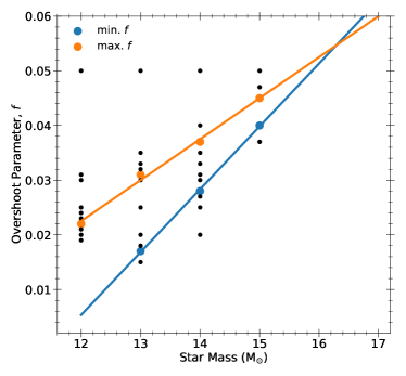
Figure 2: The grid of $f$ values for each mass is shown with circles. The orange and blue circles show the maximum and minimum $f$ values that undergo a blue loop, respectively. The two fitted lines show that these $f$ values increase linearly with mass. The models with masses larger than about 16 M_☉, where the two lines intersect do not undergo a blue loop for any choice of the $f$ value.

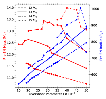
Figure 3: The final pre-supernova masses and radii as a function of overshoot parameter plotted for different zero-age main-sequence masses in the range of 12–15 M_☉.

4 Method of Simulation of Massive Star Evolution

We use MESA version r-10398 to explore models of progenitor stars of type IIP supernovae, such as SN 2013ej. In our Paper I, we explored effect of overshoot parameter $f$ on stellar properties and evolution for a model star with initial mass of 13 M_☉ at ZAMS, with initial metallicity Z = 0.006. In this paper we expand the parameter space . In addition to the 13 M_☉ star (see Paper I for details), we use an expanded grid of stellar masses and overshoot parameter, $f$ (see Fig 2 and Table 2 for the grid points of mass and exponential overshoot factor $f$ explored). We use the same metallicity, mass and temporal resolution controls, mass loss rate ($\eta_{Dutch}$=0.5), nuclear reaction network of 79 isotopes, convection with Ledoux criterion ($\alpha_{MLT}$ = 2), and semiconvection ($\alpha_{SC}$ = 0.1) as in the case of the 13 M_☉ star in Paper I. We vary the overshoot parameter for exponential decay $f$, keeping the value of other parameter $f_{0}$ constant at 0.005. We have listed all of the models between a mass range of 12–24 M_☉ and a range of values of overshoot parameter $f$ for each mass in Table 2. Only the models that have converged from the pre-main-sequence to either the core-collapse stage or within a day to core-collapse stage (which does not affect the overall RSG lifetimes) are listed in this Table. Some of the models that failed to converge soon after core-He-depletion stage due to various reasons were not useful for calculating the red supergiant time-scales to determine the B/R ratio and are thus not reported in this Table.

5 Results

5.1 Model time-scales in the supergiant phases and B/R ratio calculation

In Fig. 1, we have plotted the model evolutionary tracks in the mass range of 12 to 15 M_☉ with maximum and minimum model $f$-values that undergo a blue loop for each mass (see Table 2). The observational data is overlaid on the tracks in the right panel of Fig. 1. The two horizontal (black-dashed) lines show the luminosity range used to restrict the observational data for comparison with the model calculations of B/R and Y/R ratios. We choose this range of 4.2 $<$ $log_{10}(L/L_{\odot})$$<$ 5.0 for limiting the observational data, as this is the range covered by the model evolutionary tracks that is most appropriate for the comparison. With this luminosity limit we have 97 BSG, 87 YSG and 430 RSG candidates as noted in the last row of Table 1. These values are used to compute the observed B/R and Y/R ratios listed in Table 3.

In Table 2, we list the time-scales calculated for our models in the B/Y/RSG phases as defined in section 3. The models that undergo a blue loop go through each of these phases several times, red-ward and blue-ward. $\rm\tau_{B_{1}}$, $\rm\tau_{Y_{1}}$, $\rm\tau_{R_{1}}$ time-scales represent the first time after TAMS phase when the star is in the B/Y/RSG phases, respectively, on the red-ward track in the HRD. For the models that do not undergo a blue loop, these are also the total time-scales spent in each of these phases. For the blue loop models, several such time-scales are listed in the table for each consecutive transition. $\rm\tau_{Y_{2}}$ represents the time-scale in YSG phase when the star is on the blue-ward track on the blue loop. $\rm\tau_{B_{2}}$ represents the time-scale for the BSG phase when the star is in the blue region ($log_{10}(T_{eff}/\rm K)$ $>$ 3.875). This includes both the red-ward and blue-ward tracks including the loop. $\rm\tau_{Y_{3}}$ represents the time-scale when the star is in the YSG phase on the red-ward track in the blue loop. The star then enters the RSG phase and remains in this spectral class until core-collapse stage. This time-scale is represented by $\rm\tau_{R_{2}}$. The total time-scales in each of the B, Y, & RSG phases are then listed as the sum of the above individual time-scales in columns BSG, YSG, and RSG, respectively. The ratios of the total time-scales in the BSG to the RSG and the YSG to the RSG phases are also listed in Table 2 for comparison in the columns $\rm\tau_{BSG}/\tau_{RSG}$ & $\rm\tau_{YSG}/\tau_{RSG}$, respectively. Since the observational data from Neugent et al. (2012b) is complete only up to $T_{eff}$ $\approx$ 10,000 K, we also calculate BSG time-scales in the limit of 4.0 $\geq$$log_{10}(T_{eff}/\rm K)$$>$ 3.875 for each of our models for comparison with the observations. The total BSG time-scales in this restricted temperature range are marked as BSG^∗ in Table 2. The corresponding ratio of individual blue to red time-scales is also listed in the column $\rm\tau_{BSG^{*}}/\tau_{RSG}$.

We note that in the Neugent et al. (2012b) data, the LMC stars are predominantly field stars. Since the field stars do not co-evolve like those in the clusters, we can assume a stellar population in a steady state with a constant star formation rate. We can thus evaluate the B/R ratio in terms of the relative duration of the two supergiant phases. For constant star formation rate, the B/R ratio (Ekström et al., 2013, $N_{B}/N_{R}$,) can be modified for discrete mass values as :

$$\frac{N_{B}}{N_{R}}=\frac{\int\limits_{m}\tau_{B}(m)\ \phi(m)\ dm}{\int\limits_{m}\tau_{R}(m)\ \phi(m)\ dm}$$ (2)

where $\phi(m)=(dN/dm)\propto m^{-\alpha}$ is the initial mass function with slope $\alpha=-$2.35 (Salpeter, 1995). However, we find from our model predictions that the supergiant time-scales, and hence, the B/R ratio are also dependent on the convective overshoot parameter $f$ for a given mass (see Table 2 for time-scales). Thus we introduce the $f$-dependence of the ratio in equation 2 as

$$\frac{N_{B}}{N_{R}}=\frac{\int\limits_{m}\phi(m)\ dm\int\limits_{f}\tau_{B}(m,f)\ P(f)|_{m}\ df}{\int\limits_{m}\phi(m)\ dm\int\limits_{f}\tau_{R}(m,f)\ P(f)|_{m}\ df}$$ (3)

where $P(f)|_{m}$ is a probability function for finding stars with a particular $f$ for a given mass. The nature of convective overshoot and its mass dependence is not known, and hence, $P(f)$ cannot be well determined. As trials, we use two different forms of the probability functions to calculate the B/R & Y/R ratios – (1) $P(f)=constant$ (i.e. all $f$ values are equally probable) and (2) a normalized Gaussian of the form

$$P(f)=\frac{1}{\sqrt{2\pi\Delta^{2}}}e^{-((f-f_{c})/2\Delta)^{2}}$$ (4)

where, $f_{c}$ is the “central” value and $\Delta$ is the “width” of the Gaussian.

We see from Figure 2 that the models that exhibits a blue loop are bound between two extreme values of the overshoot parameter, $f$. Furthermore, these two extreme values appear to vary linearly with mass (orange and blue lines in the figure). We see that these two lines intersect at around 16.3 M_☉, above which the models would not undergo a blue loop for any $f$ value in our selected range. As pointed earlier, the models that undergo a blue loop spend a significant amount of time in the BSG phase, compared to the models that do not undergo a blue loop. Hence, the number of BSG stars seen in the observations would be dominated by the models that undergo a blue loop. We choose the central value $f_{c}(m)$ for the Gaussian probability function $P(f)|_{m}$ at the maximum $f$ value for each mass that exhibits a blue loop (orange circles in Figure 2), which follows the (orange) line such that

$$f_{c}(m)=0.0075m-0.0675$$

We choose the $\Delta$ (“width”) for the Gaussian to be equal to half of the difference between the minimum and maximum $f$ values (orange and blue circles in Figure 2) for each mass. We evaluate the normalized Gaussian probability function $P(f)$ over a range of $f$ values between 0.01 and 0.05. However, we only use the time-scales from the models that undergo a blue loop for the ratio calculation, for the reason mentioned above.

To calculate the B/R ratio, we use the trapezoidal method to evaluate the integral in equation 3 for discrete values of $m$ and $f$. We get B/R = 0.15 for both the constant $P(f)$ and the Gaussian $P(f)$. We also calculate Y/R ratio using same methodology to yield Y/R = 0.044 and 0.058, respectively, for constant and Gaussian $P(f)$. We also compute the ratio of blue+yellow supergiants to red supergiants (B+Y)/R = 0.19 and 0.21, respectively, for constant and Gaussian $P(f)$. These values are listed in Table 3. We infer from these results that the choice for the form of the probability function $P(f)$ has a minimal effect on the predicted B/R and Y/R ratios.

Table 3: The observed and predicted B/R & Y/R ratios

ratio	Observed	Observed∗	Predicted
			constant $P(f)$	Gaussian $P(f)$
B/R	097/430=0.23	0.14	0.150	0.150
Y/R	087/430=0.20	0.13	0.044	0.058
(B+Y)/R	184/430=0.42	0.26	0.190	0.210

Note. — The observed supergiant candidates in the Neugent et al. (2012b) data are selected based on their LMC membership. The blue, yellow, and red supergiants (B/Y/RSG) are then separated based on their effective temperature using the criteria described in section 3. Furthermore, the candidates that have 4.0 $<$ $log_{10}(L/L_{\odot})$$<$ 5.0 are selected to calculate the observed ratios listed in this table (see last row in Table 1). The column marked with asterix (*) shows a modified observed ratio if we include the 60% missing dust-enshrouded RSGs as discussed in section 3.4 . The predicted ratios are calculated using model time-scales for stars with masses in the range of 12–15 M_☉, as explained in section 5.1. $P(f)$ is a probability function of finding a star with a particular $f$ value for a given mass.

5.2 Pre-Supernova Radii and Final Masses

As we have explored the evolution of massive stars starting with different initial masses and (exponential) overshoot factors, we find that the luminosity of a given star is highly dependent on the above variables at any given evolutionary stage (e.g. the Terminal Age Main Sequence (TAMS), the horizontal transition from the BSG to the RSG phase, the He-ignition stage, etc.). This is evident from our Figure 1 (or the Figure 1 of our Paper I). Depending on the mass and the overshoot factors, the stars spend different fractions of their post-TAMS lifetimes in either the RSG phase or the other hotter phases. The mass loss rates from the star is known to be sensitively dependent on both Luminosity and $T_{eff}$ (see for example figure 6 of Wagle & Ray, 2020, and the references listed therein). For a star of a given mass and an overshoot factor, the mass lost from it up to the core-collapse stage depends mainly on the fractional duration that the star spends in the RSG phase. It is in this phase that the mass loss rate is particularly high. As the total post-main-sequence lifetime, as well as, the fractional duration in the RSG phase depend on the initial mass and the overshoot factor, it is evident that the final mass of the star before core collapse would be different.

In Figure 3, we show the final masses and the final radii of the stars as a function of the overshoot factor for different initial masses. For certain combination of masses and overshoot factors, the star spends long time in the hotter phases due to the blue loops. If the star lacks blue loops altogether, it would end up losing more mass. It will then end up with low final mass than it otherwise would, as seen for initial masses 13 M_☉, 14 M_☉, and 15 M_☉ star. The final radius tends to vary monotonically with the overshoot factor by nearly a factor of two for certain initial masses (12 M_☉ and 13 M_☉).

6 Discussion and Conclusion

In this work, we have presented models for progenitors of Type IIP supernovae, using nearby, well-observed SN 2013ej in the host galaxy M74 for an example. The metallicity of the neighboring Hii region 197 of SN 2013ej is determined to be 0.006 (Cedrés et al., 2012), which is similar to that of the LMC. We therefore investigate the evolution of the progenitor star in a low Z environment up to the pre-supernova stage using the Ledoux criterion for convection and near-standard mass loss rate predicted for hot and cool stars. In continuation of our previous papers in this series, we study the effects of convective overshoot on the model predicted B/R ratio in this paper. We try to determine how well the model properties reproduce the observed B/R ratio for the LMC.

The luminosity of supergiant star is affected by both its initial mass, as well as the extent of overshooting. Thus, we explore a grid of masses and overshoot factors. We find that the key feature displayed by these models in the HR diagram is the blue loop (see our Paper I for an analysis.) There is a range of overshoot parameter ($f$) values that for a given intital mass exhibit the blue loop behavior. However, outside of this range, the blue loops disappear. In addition, the maximum and minimum values of $f$ that exhibit a blue loop follow a linear trend in mass (as seen in Fig. 1). The blue loop is not exhibited in the models with initial masses higher than about 16 M_☉. This is also seen in the figure, where the two lines (orange and blue) fitted to the maximum and the minimum $f$ values that undergo a blue loop intersect. The existence of the blue loop is in fact critical for accounting the observed number of BSG stars. The models that undergo a blue loop spend a substantial amount of time in their post-TAMS lifetime at relatively higher effective temperature regions. In contrast, the models with higher or lower $f$ values transit quickly to RSG branch and spend their entire post-core-helium-ignition lives in the RSG stage.

The observations by Neugent et al. (2012b), however, only extend to a maximum $T_{eff}$ of about 10,000 K. Therefore, we subdivided the supergiant region into the blue, yellow, and red regions based on the effective temperature. We use these criterion for determining the B/R and Y/R ratios for both the observations as well as the model predictions. We have determined the B/R and Y/R ratios predicted by our non-rotating stellar models in the mass range of 12–15 M_☉, using the formulation explained in section 5.1. We are able to match very well the observed B/R ratio in the LMC, especially if we include the 60% missing RSGs that might be dust-obstructed (see section 3 and Table 3, for comparison). However, the Y/R ratio is under-predicted by our models within a factor of $\sim$2 in comparison to the observations. If we group together the observed B+YSG stars then the predicted (B+Y)/R ratio comes within a good agreement within a few tens of percent. We would also like to note that we have chosen all of the B/Y/RSG stars present in the data within the chosen luminosity range for calculating the ratios. However, the spectral types are not determined for all of these stars, especially most of the RSG candidates. In fact, if we were to choose the spectroscopically identified candidates only for our calculations, then we would have about 85-95 % of the yellow and blue supergiant candidates available to us from the data. However, we would account for only about 14% of the total number of RSG candidates. Thus, selecting only the spectroscopically identidied candidates would skew the B/R and Y/R ratio to a higher side (a value $>$ 1). However, it would not be a correct comparison as many genuine RSG candidates would be neglected in such case.

In this paper, we have explored predictions for both mass and overshoot factors affecting the stellar luminosity and temperatures at different stages of its evolution through model calculations and used the lifetimes in specific segments of the HRD to compute the B/R or the Y/R ratios implied from these model calculations. Our attempts to match these predictions with observations of supergiants in the LMC are largely successful. Blue loops due to their long lifetimes of these phases are important elements in matching the model predictions to observations. The predictions of blue loops in the HRD for certain ($M,f$) ranges implies that the extent of the overshoot for which blue loops are found are bounded between two extreme $f$ values which may in turn be intensifying with the initial mass $M$ (see Figure 2).

Final masses and radii of the presupernova star affect the post explosion dynamics and development of light curves and spectra significantly. They control the optical, IR display of the type IIP supernovae through both the amount of hydrogen left on the star at explosion stage as well as the radius $R(0)$ at shock breakout phase (which depends on the final presupernova radius $R_{fin}$ itself). For example the luminosity of the supernova at the plateau phase can be written as (see equation (64) of Arnett, 1980):

$$L\propto R(0)v_{sc}^{2}$$

where $v_{sc}$ is a constant that sets the velocity scale (see Arnett, 1980, equation (5)) and may depend upon the kinetic energy and mass of the star and their distributions at the time of shock breakout. Thus, the convective overshoot factor of the pre-supernova star is expected to affect significantly the luminosity and spectral properties in the post-supernova stage. Note that the spectral evolution of the developing supernova including its line properties is controlled by $v_{sc}$. In a future paper, we shall explore in detail how the convective overshoot affects the model light curves and spectra of a supernova, through the mass, radii and velocity scales controlled by the energy of explosion.

References

- Arnett (1991) Arnett, D. 1991, ApJ, 383, 295
- Arnett (1980) Arnett, W. D. 1980, ApJ, 237, 541
- Arnett et al. (1989) Arnett, W. D., Bahcall, J. N., Kirshner, R. P., & Woosley, S. E. 1989, ARA&A, 27, 629
- Brunish et al. (1986) Brunish, W. M., Gallagher, J. S., & Truran, J. W. 1986, AJ, 91, 598
- Brunish & Truran (1982a) Brunish, W. M., & Truran, J. W. 1982a, ApJ, 256, 247
- Brunish & Truran (1982b) Brunish, W. M., & Truran, J. W. 1982b, ApJS, 49, 447
- Castro et al. (2014) Castro, N., Fossati, L., Langer, N., et al. 2014, A&A, 570, L13
- Cedrés et al. (2012) Cedrés, B., Cepa, J., Bongiovanni, Á., et al. 2012, A&A, 545, A43
- Choi et al. (2016) Choi, J., Dotter, A., Conroy, C., et al. 2016, ApJ, 823, 102
- Davies et al. (2018) Davies, B., Crowther, P. A., & Beasor, E. R. 2018, MNRAS, 478, 3138
- Dorda et al. (2016) Dorda, R., Negueruela, I., González-Fernández, C., & Tabernero, H. M. 2016, A&A, 592, A16
- Drout et al. (2009) Drout, M. R., Massey, P., Meynet, G., Tokarz, S., & Caldwell, N. 2009, ApJ, 703, 441
- Eggenberger et al. (2002) Eggenberger, P., Meynet, G., & Maeder, A. 2002, A&A, 386, 576
- Ekström et al. (2013) Ekström, S., Georgy, C., Meynet, G., Groh, J., & Granada, A. 2013, in EAS Publications Series, Vol. 60, EAS Publications Series, ed. P. Kervella, T. Le Bertre, & G. Perrin, 31–41
- Farrell et al. (2020) Farrell, E. J., Groh, J. H., Meynet, G., & Eldridge, J. J. 2020, MNRAS, 494, L53
- Fitzpatrick & Garmany (1990) Fitzpatrick, E. L., & Garmany, C. D. 1990, ApJ, 363, 119