Classification of Equation of State in Relativistic Heavy-Ion Collisions Using Deep Learning

Abstract

Convolutional Neural Nets, which is a powerful method of Deep Learning, is applied to classify equation of state of heavy-ion collision event generated within the UrQMD model. Event-by-event transverse momentum and azimuthal angle distributions of protons are used to train a classifier. An overall accuracy of classification of 98% is reached for Au+Au events at $\sqrt{s_{NN}}=11$ GeV. Performance of classifiers, trained on events at different colliding energies, is investigated. Obtained results indicate extensive possibilities of application of Deep Learning methods to other problems in physics of heavy-ion collisions.

1 Introduction

One of the main goals of physics of heavy-ion collisions is to explore properties of exotic state of matter, namely, hot, dense and hard-interacting baryonic matter. It can be recreated in laboratory by colliding heavy nuclei at relativistic energies. Lattice Quantum Chromodynamics (QCD) calculations indicate that a transition from quark-gluon plasma (QGP) to hadron gas is a smooth crossover at high energies and low baryon densities lattice . It is widely believed that a first-order phase transition that ends up with tricritical point takes place within the energy range between $\sqrt{s}=3$ and 10 GeV, see, e.g., phdiagram and references therein. Various past and ongoing experiments, such as beam energy scan (BES) and BES II at Relativistic Heavy Ion Collider (RHIC) besI ; besII , experiments at Super Proton Synchrotron (SPS) at CERN, are exploring collisions with gold and lead ion beams to find any peculiarities within the aforementioned energy range. However, neither the first-order phase transition, nor the tricritical point has been observed so far. Future experiments, such as Nuclotron-based Ion Collider fAcility (NICA) and Facility for Antiproton and Ion Research (FAIR) are aiming to perform collisions at given energies with higher luminosity, which give us a hope to see something new there. Difficulties in observing the phase transition originate from numerous factors. Some of them are an extremely short, approximately $10^{-24}$ fm/$c$, time of existence of the QGP phase, small number of particles in the system, high anisotropy of matter both in coordinate and in momentum space, etc. All valuable information registered by detectors is roughly several thousands of particles with corresponding energies and momenta. Therefore, it is immensely difficult to make any reasonable assumptions about the media they came from.

Recent success of methods of Artificial Intelligence (AI), such as Machine Learning (ML) and Deep Learning (DL), in approximating highly obscure dependencies gives us a justifiable hope that they can benefit in heavy-ion physics objectives. Now these methods are widely employed in various problems that involve pattern recognition, for instance, image classification, natural language processing, and so on. Major advantage of such algorithms is that they do not need to be explicitly programmed. For example, AlphaGo alphago , a program developed by Google Deep Mind to play a board game Go, managed to beat human world champion with the score 4:1. Played on 19x19 board, Go has roughly $2.08*10^{170}$ legal positions which makes it impossible for explicitly-written algorithm due to computational complexity. Moreover, a more advanced versions of the program, AlphaGo Zero and AlphaZero, were trained even without using the human data or guidance, but only by playing between versions of themselves and reached even better results alphago2 . Recently, algorithms of DL have started to be applied to complex tasks in various fields of physics, namely, high-energy particle physics taudl ; jetdl ; partojetdl , condensed matter physics manybodyann ; vrgdl , astroparticle physics cosmicraydl ; astrophdl ; exopldl , and quantum information alphazq . The work physconcdl demonstrates how optimal representation variables, describing different states of physical systems, could be learned by neural nets. Generative Adversarial Nets, a generative Deep Learning models have started to be successfully applied for the event simulations jetgan ; muongan . Review of possibilities of application of ML and DL methods to high energy physics can be found elsewhere mlreview1 ; mlreview2 ; mlreview3 . Prominent results of application of DL to problems of high energy nuclear physics and heavy-ion collisions are described in eosdl ; qcdtransitdl ; spinoclumpml .

Present work continues efforts of application of deep learning methods to identification of properties of equation of state (EoS). The paper is organized as follows. Section 2 introduces basic features of the microscopic ultrarelativistic quantum molecular dynamics (UrQMD) model and parameters of hard and soft mean-field potentials used in the calculations. It is outlined that the Deep Learning methods are able to differentiate the calculations made with two different equations of state on event-by-event basis compared to standard methods, which need usually significant statistics of generated events. Principles of the Convolutional Neural Network (CNN) algorithm are sketched in Sec. 3. Section 4 presents main results of our study. Here we show also the ability of model, trained on particular collision energy, to make correct distinctions for the collisions at neighbor energies. Effectiveness of different training algorithms is discussed as well. Conclusions are drawn in Sec. 5.

2 Work Setup

2.1 Features of microscopic model

The Ultra-relativistic Quantum Molecular Dynamics model urqmd_1 ; urqmd_2 is a Monte-Carlo event generator designed for the description of $hh$, $hA$, and $A+A$ collisions in a broad energy range from hundred MeV up to several TeV. The model contains 55 baryon and 32 meson states with masses up to 2.25 GeV/$c^{2}$ as independent degrees of freedom, together with their antiparticles and explicit isospin-projected states. At energies below few GeV, the interaction dynamics of $hh$ or $A+A$ collisions can be described via interactions between the hadrons and their excited states, resonances. At higher energies new processes of multiparticle production come into play. The UrQMD treats the production of new particles via formation and fragmentation of specific colored objects, strings. Strings are uniformly stretched between the quarks, diquarks and their antistates with constant string tension $\kappa\approx 1$ GeV/fm. The excited strings are fragmenting into pieces via the Schwinger mechanism of $q\bar{q}$-pair production, and the distribution of newly produced hadrons is uniform in the rapidity space. The model utilizes Hamiltonian dynamics of particle motions and incorporates particle interaction via geometric cross sections, taken from available experimental data or from quark models.

2.2 Hard and soft EoS

There is a possibility to switch-on potential interaction in the form of Yukawa, Coulomb, and Skyrme potentials

$$V=\sum_{i\neq j}\left(V^{Yuk}_{0}\frac{e^{-|\vec{r}_{i}-\vec{r}_{j}|/\gamma_{Y}}}{|\vec{r}_{i}-\vec{r}_{j}|}+\frac{Z_{i}Z_{j}e^{2}}{|\vec{r}_{i}-\vec{r}_{j}|}\right)+t_{1}\rho^{int}_{j}+t_{\gamma}(\gamma+1)^{-3/2}(\rho^{int}_{j})^{\gamma}\ ,$$ (1)

where

$$\rho^{int}_{j}=\left(\frac{\alpha}{\pi}\right)^{3/2}e^{-\alpha r_{j}^{2}}$$ (2)

Here $\vec{r_{i}}$ is a coordinate vector of $i$-th particle, $Z_{i}$ is value of electric charge, $\rho^{int}_{j}$ is interaction density, $V^{Yuk}_{0},\ \gamma_{Y},\ t_{1},\ t_{\gamma},\gamma$ are constants that define stiffness of EoS, see urqmd_1 ; urqmd_2 ; pot for details. In present work we use potential with two different sets of parameters which can be associated with two separate equations of state, hard and soft, of baryonic matter. Parameters of the hard and the soft potentials employed in the calculations are listed in Table 1.

Parameter	Hard potential (EoS1)	Soft potential (EoS2)
$\alpha$	0.25	0.25
$t_{1}$	-163	-353
$t_{\gamma}$	125.93	304
$\gamma$	1.676	1.167
$V^{Yuk}_{0}$	-0.498	1.0038
$\gamma^{Yuk}$	1.4	1.4

Table 1: Parameters of the hard and soft mean-field potentials used in the current version of the UrQMD.

2.3 Example: directed flow

It was shown earlier that EoS in UrQMD influences kinematic observables, such as directed flow, $v_{1}$, quite significantly flow . Recall, that directed flow volflow is an experimental observable that characterizes momentum space anisotropy of particle spectrum. It is defined as first coefficient of transverse flow Fourier decomposition

$$\displaystyle E\frac{d^{3}N}{d^{3}p} = \frac{d^{2}N}{\pi dp_{T}^{2}dy}\Bigg{\{}1+2\sum\limits_{n=1}^{\infty}v_{n}\cos{\left[n(\phi-\Psi_{n})\right]}\Bigg{\}}~{},$$ (3)

$$v_{n} = \langle\cos{\left[n(\phi-\Psi_{n})\right]}\rangle~{}.$$ (4)

Here $p_{T}$ is particle transverse momentum, $y$ is rapidity, $\phi$ is the azimuth between the $\vec{p_{T}}$ and the participant event plane, and $\Psi_{n}$ is the azimuthal angle of the event plane of $n$-th flow component. Averaging in Eq. (4) is done over all particle of a given species from the single event and over all set of events.

Figure 1 shows the midrapidity slopes of directed flow of protons in minimum bias Au+Au collisions at energies $\sqrt{s}=4,\ 7.7,\ 11.5,\ 19.6$ GeV generated with two different EoS. One can see that the value of the slope is sensitive to the choice of EoS. However, to make the differences in $v_{1}$ slopes visible, about one million events for each data point were needed.

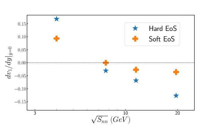
Figure 1: Slope of directed flow of protons coming from UrQMD minimum bias Au+Au collisions generated with hard (stars) and soft (crosses) EoS, respectively. Data are taken from flow .

2.4 Model setup

It is worth mentioning that application of the Deep Learning methods permits one to differentiate between EoS on event-by-event basis. To check the efficiency of the method we generated 5000 Au+Au collisions of each kind at $\sqrt{s}=11$ GeV with centrality 0-5%. Distribution of proton number $n_{p}=n_{p}(p_{T},\phi)$ was calculated for each separate event. Transverse momentum and azimuthal angle were selected in ranges (0,1) GeV/$c$ and (-$\pi$,$\pi$), respectively. Altogether, the training dataset is consisted of 10000 histograms with dimensions of $10\times 10$ bins and labeled "0" for hard potential and "1" for soft potential. All bin values were scaled to fit the range (0,1), so they represent probability density distribution.

3 Deep Convolutional Neural Network

Convolutional Neural Network (CNN) CNN has proven to be a powerful deep learning algorithm for tasks dealing with graphical data, such as image recognition, classification, etc. It was inspired by the process of image processing in mammal’s visual cortex. Similar to other deep learning algorithms, CNN consists of layers of artificial neurons. However, there are three main types of layers that are used in deep CNN. Convolutional layers are used to extract useful features. Pooling layers are responsible for reduction of parameters and fully-connected ones are used for making the final prediction. They map extracted features to the desired output, which is either "1" or "0" in our case. Configuration of layers is determined by the complexity of the task. Network architecture employed here is described in Table 2 and visualized in Fig. 2, build with the help of online tool for CNN architecture visualization .

No.	Layer	Parameters
0.	Input	1x10x10 tensor
1.	Conv2D	8 kernels 3x3, ReLU
2.	MaxPool2D	2x2 kernel, stride 2
3.	Conv2D	2 kernels 3x3 , ReLU
4.	MaxPool2D	3x3 kernel, stride 1
5.	FullyConnected	144 neurons, ReLU
6.	FullyConnected	36 neurons, ReLU
7.	Sigmoid

Table 2: Architecture of Convolutional Neural Network.

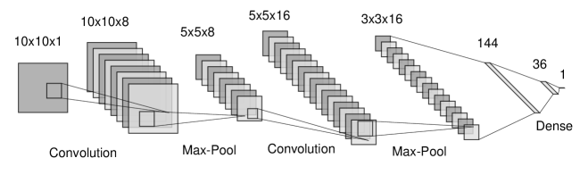
Figure 2: Network architecture diagram.

Binary cross-entropy, used as a loss function, reads

$$S=-w_{n}\left(y_{n}*\log{(x_{n})}+(1-y_{n})*\log{(1-x_{n})}\right)$$ (5)

Here $w_{n}$ is a sample weight (set to 1), $x_{n}$ and $y_{n}$ are network outputs and true labels, respectively. Index $n$ runs over the batch. The network was trained with a help of stochastic gradient descent (SGD) method with learning rate 0.01 during 800 epochs. Dropout dropout layers (p=0.3) were used before every fully-connected layer to reduce overfitting. Validation loss was recorded after every 10 epochs and model parameters were saved every time it decreased. Model parameters that yielded lowest loss at validation set were used for model evaluation afterwards. Eighty percent of the dataset was used for training and twenty percent for validation. Data acquisition and early preprocessing steps were done within the ROOT framework root . Further process was realized in Jupyter-lab jupyter-lab , which is an interactive Python notebook, with an extensive use of the Python libraries NumPy numpy_1 ; numpy_2 , Matplotlib matplotlib , Pandas pandas , and Scikit-learn skl . The network was realized in PyTorch pytorch framework.

4 Results

4.1 Classification accuracy for central Au+Au collisions at three different energies

Typical particle density profiles coming from events generated with both hard and soft potentials are shown in Fig. 3.

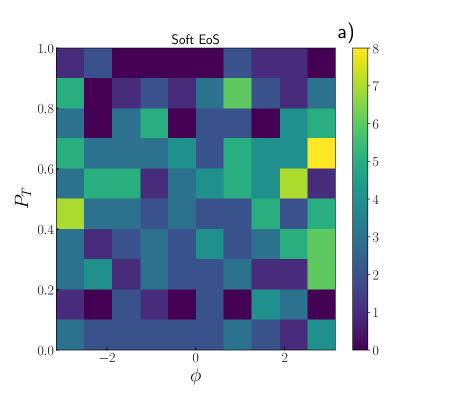
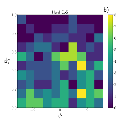
Figure 3: Proton densities for (a) soft and (b) hard potentials from a single UrQMD generated Au+Au collision at $\sqrt{s}=11$ GeV.

We have to emphasize that density profiles from single event are strongly influenced by fluctuations and substantially differ on event-by-event basis. They are hardly distinguishable by naked eye, yet if we consider larger statistics, e.g., 100 events, the differences become more noticeable, as shown in Fig. 4.

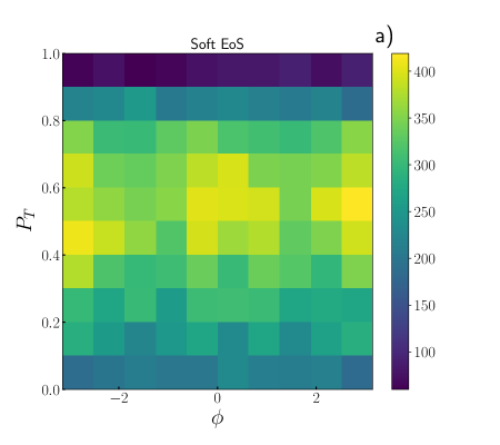
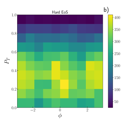
Figure 4: The same as Fig. 3, but for 100 Au+Au collisions.

Overall classification accuracy of 98% percent was achieved for both hard and soft potentials. It means that out of 100 items of every kind 98 were classified correctly. Learning curves are depicted in Fig. 5. One can see that after 100-th epoch both training and validation losses start to abruptly fall, whereas both accuracies rapidly grow. This circumstance indicates that a direction of minimum of loss function in the model parameter space is found. All curves enter the saturation region after 150-th epoch. The fact that training metrics coincides with validation metrics indicates that our model does not overfit and generalizes well.

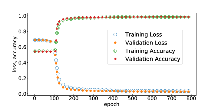
Figure 5: Training and validation losses and accuracies for UrQMD generated Au+Au collisions at $\sqrt{s}=11$ GeV

Then, analogous setup was used for energies of $\sqrt{s}=7$ and 14 GeV. For the last case overall accuracy of 98% was reached, however, it drops to 94% of accuracy for $\sqrt{s}=7$ GeV collision energy within the proposed training scheme. It could be attributed to low multiplicity of secondary particles, produced in a single event. Next, it is interesting to study the ability of a model, trained on one particular energy, to make predictions for another energy. These results are listed in Table 3. There are three trained models together with their predictions for Au+Au collisions at three energies, $\sqrt{s}=7,\ 11,$ and 14 GeV. Table 3 reveals an interesting result that a classifier, trained on events at collision energy of $\sqrt{s}=14$ GeV, shows good performance while classifying the events at lower energies. The same is true for the classifier trained at $\sqrt{s}=11$ GeV. It could indicate on similarities in hadron spatial distributions in both reactions. In contrast, performance of the classifier trained on $\sqrt{s}=7$ GeV is significantly worse. Possible explanation could be low particle yields in a single event at this energy which are not enough to make a distinction properly.

Training energies	Efficiency (%)
$\sqrt{s}$ (GeV)	7	11	14
7	94	55	50
11	77	98	90
14	74	96	98

Table 3: Performance of models trained at different energies.

As it turned out, the smallest amount of data needed for accuracy better than 96% is only 100 images, i.e., only 1% of the whole dataset, for energies $\sqrt{s}=11$ and 14 GeV. For the energy of 7 GeV the best performance with the least amount of data used is 92% with 400 training instances. However, training time is roughly 5 times longer compared to 4000 epochs for $\sqrt{s}=11$ GeV.

4.2 Application of more efficient algorithm - Adam

It is possible to achieve very good results, namely, 92% of accuracy on validation set for $\sqrt{s}=7$ GeV and 96% of accuracy on validation set for $\sqrt{s}=11$ and 14 GeV, by using the Adam routine Adam , which is a more advanced algorithm of loss minimization. Figure 6, Fig. 7, and Fig. 8 show overall validation accuracy during 5000 epochs of training for three energy data sets with different amount of training data and different optimizers.

Figure 6: Validation loss during 5000 epochs of training for different training data fractions and optimizers in Au+Au central collisions generated within UrQMD at $\sqrt{s}=7$ GeV. Solid and dashed curves indicate the results obtained by SGD method with train fraction 4% and 20%, respectively. Dotted curve denote the results obtained by Adam method with 4% train fraction.

Results obtained for central Au+Au collisions at $\sqrt{s}=7$ GeV are displayed in Fig. 6. To reach the desired accuracy above 90% by standard SGD method using just 4% of generated statistics as a train factor, one needs about 2500 epochs. This time can be shortened to approximately 600 epochs if 20% of events are used for the training. In contrast, application of the Adam algorithm with 4% train fraction needs only 30(!) epochs to reach the accuracy about 90%. Peculiarity in application of this method is the slow declining of the validation accuracy after 100 epochs, which means that the model starts to overfit. Recall that training with low amounts of data is unstable with both training algorithms. More time is required by the model to find a path to the minimum of the loss. The problem can be cured by increase of the training statistics. It is important because the multiplicity of produced hadrons in heavy-ion collisions drops with decreasing collision energy. For Au+Au collisions at $\sqrt{s}=11$ and 14 GeV the multiplicities of secondaries are larger than that at $\sqrt{s}=7$ GeV.

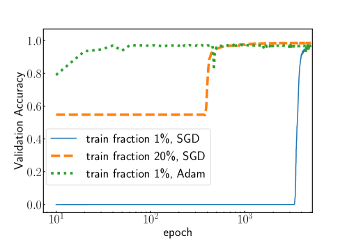
Figure 7: The same as Fig. 6 but for central Au+Au collisions at $\sqrt{s}=11$ GeV.

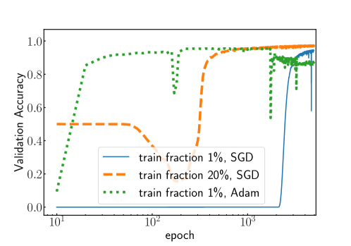
Figure 8: The same as Fig. 6 but for central Au+Au collisions at $\sqrt{s}=14$ GeV.

Here advantages of the Adam algorithm become more obvious, as shown in Fig. 7 for the collisions at $\sqrt{s}=11$ GeV. The standard SGD optimization method demonstrates sharp increase of the validation accuracy after 3200 epochs for the train fraction 1%, and after 400 epochs for the train fraction 20%. Training with Adam algorithm converges much faster. We see a rapid increase of accuracy in EoS recognition with the train fraction 1% after 30 epochs already. The same efficiency is obtained for central Au+Au collisions at $\sqrt{s}=14$ GeV, as depicted in Fig. 8. Therefore, a classificator trained with the Adam optimization algorithm needs very limiting statistics for training within quite short time to discriminate between the hard and the soft equation of state with accuracy about 95%.

5 Conclusions and Discussion

Our main results can be summarized as follows. Convolutional Neural Networks demonstrate excellent performance for equation of state classification in UrQMD generated heavy-ion collisions. Binary classification accuracy of 98% is achieved for events at $\sqrt{s}=11$ and 14 GeV and 94% for $\sqrt{s}=7$ GeV, using the data set of primitive experimental observables, such as particle transverse momentum and azimuthal angle. Moreover, it is possible to differentiate between equation of state using the model trained on different neighboring energies.

It turned out that even a small fraction of data is enough to achieve satisfactory results. Training time depends strongly on data fraction used for the training, and on the employed algorithm. Our study shows that to reach the top classification accuracy for central Au+Au collisions at energies about 11 GeV and higher by the standard Stochastic Gradient Descent method, one needs more that 3000 epochs for training data of 1% of the generated statistics, and more than 400 epochs if the training fraction was increased to 20%. Similar accuracy can be achieved by application of the stochastic optimization algorithm Adam trained at statistics of 1% just after 30 epochs. Therefore, training Convolutional Neural Network classifier with the Adam algorithm permits one to reach high accuracy during very short training time with little amount of training data.

It is worth mentioning that the performance of trained CNN routine is very robust against initial state fluctuations and final state interactions, such as decays of resonances. However, similar to other applications of DL technique to high energy physics eosdl ; qcdtransitdl ; spinoclumpml , the program has to decide between two discrete choices: calculations either with soft or stiff equation of state. In other words, this is a one-dimensional discrete space. In reality, the space of possible EoS is continuous. The next step, therefore, should be calculations with a combined EoS containing certain fraction $x$ of the soft EoS and complementary fraction $1-x$ of the stiff EoS. The model trained on such data would definitely give us fractions of both EoS. It will take more time because of the amount of generated data and longer training procedure. But, as we show in our study, the application of sophisticated algorithms, like Adam, makes solving this problem possible.

After that one can make a transition to multi-dimensional continuous space. This will allow us to extract different parameters of the EoS provided we can fix its functional form. If the limits of values of each parameter, entering the EoS, are determined, we have to generate the events for each set of parameters. Then, we train the model so that it learns the correspondence between $(p_{T},\phi)$-distributions of hadrons and set of parameters. The whole procedure looks cumbersome but feasible. This interesting problem needs further investigations.

- (1) Y. Aoki, G. Endrodi, Z. Fodor, S.D. Katz and K.K. Szabo, The Order of the Quantum Chromodynamics Transition Predicted by the Standard Model of Particle Physics, Nature 443 (2006) 675
- (2) K. Fukushima and T. Hatsuda, The Phase Diagram of Dense QCD, Rep. Prog. Phys. 74 (2011) 014001
- (3) G. Odyniec, The RHIC Beam Energy Scan program in STAR and what’s next, J. Phys. Conf. Ser. 455 (2013) 012037
- (4) D. Tlusty, The RHIC Beam Energy Scan Phase II: Physics and Upgrades, arXiv:1810.04767
- (5) D. Silver et al., Mastering the game of Go with deep neural networks and tree search, Nature 529 (2016) 484
- (6) D. Silver et al., Mastering the game of Go without human knowledge, Nature 550 (2017) 354
- (7) J. Barnard et al., Parton shower uncertainties in jet substructure analyses with deep neural networks, Phys. Rev. D 95 (2017) 014018
- (8) P. Baldi, P. Sadowski and D. Whiteson, Enhanced Higgs Boson to Search with Deep Learning, Phys. Rev. Lett. 114 (2015) 111801
- (9) CMS Collaboration (A.M. Sirunyan et al.), A deep neural network to search for new long-lived particles decaying to jets, arXiv:1912.12238
- (10) G. Carleo and M. Troyer, Solving the quantum many-body problem with artificial neural networks, Science 355 (2017) 602
- (11) P. Mehta, M. Bukov, C.-H. Wang, A.G.R. Day, C. Richardson, C.K. Fisher, and D.J. Schwab, A high-bias, low-variance introduction to Machine Learning for physicists, Phys. Rep. 810 (2019) 1
- (12) M. Erdmann, J. Glombitza and D. Walz, A Deep Learning-based Reconstruction of Cosmic Ray-induced Air Showers, Astropart. Phys. 97 (2018) 46
- (13) E.A. Huerta et al., Enabling real-time multi-messenger astrophysics discoveries with deep learning, Nat. Rev. Phys. 1 (2019) 600
- (14) C.J. Shallue and A. Vanderburg, Identifying Exoplanets with Deep Learning: A Five-Planet Resonant Chain Around Kepler-80 and an Eighth Planet Around Kepler-90, Astr. J. 155 (2018) 94
- (15) M. Dalgaard et al., Global optimization of quantum dynamics with AlphaZero deep exploration, npj Quantum Inf. 6 (2020) 6
- (16) R. Iten, T. Metger, H. Wilming, L. del Rio and R. Renner, Discovering Physical Concepts with Neural Networks, Phys. Rev. Lett. 124 (2020) 010508
- (17) R. Di Sipio, M.F. Gianelli, S.K. Haghighat and S. Palazzo, DijetGAN: a Generative-Adversarial Network Approach for the Simulation of QCD Dijet Events at the LHC, J. High Energ. Phys. 2019 (2019) 110
- (18) C. Ahdida et al. (SHiP Collaboration), Fast simulation of muons produced at the SHiP experiment using Generative Adversarial Networks, J. Inst. 14 (2019) P11028
- (19) A. Radovic, M. Williams, D. Rousseau, M. Kagan, D. Bonacorsi, A. Himmel, A. Aurisano, K. Terao and T. Wongjirad, Machine learning at the energy and intensity frontiers of particle physics, Nature 560 (2018) 41
- (20) K. Albertson et al., Machine Learning in High Energy Physics Community White Paper, J. Phys. Conf. Ser. 1085 (2018) 022008
- (21) M. Paganini, Machine Learning Solutions for High Energy Physics: Applications to Electromagnetic Shower Generation, Flavor Tagging, and the Search for di-Higgs Production, arXiv:1903.05082
- (22) L.-G. Pang, K. Zhou, N. Su, H. Petersen, H. Stöcker and X.-N. Wang, An equation-of-state-meter of quantum chromodynamics transition from deep learning, Nat. Commun. 9 (2018) 210
- (23) Y.-L. Du, K. Zhou, J. Steinheimer, L.-G. Pang, A. Motornenko, H.-S. Zong, X.-N. Wang and H. Stöcker, Identifying the nature of the QCD transition in relativistic collision of heavy nuclei with deep learning, arXiv:1910.11530
- (24) J. Steinheimer, L.-G. Pang, K. Zhou, V. Koch, J. Randrup and H. Stöcker, A Machine Learning Study to Identify Spinodal Clumping in High Energy Nuclear Collisions, J. High Energ. Phys. 2019 (2019) 122
- (25) S.A. Bass et al., Microscopic models for ultrarelativistic heavy ion collisions, Prog. Part. Nucl. Phys. 41 (1998) 255
- (26) M. Bleicher et al., Relativistic hadron-hadron collisions in the ultrarelativistic quantum molecular dynamics model, J. Phys. G 25 (1999) 1859
- (27) C. Hartnack, R.K. Puri, J. Aichelin, J. Konopka, S.A. Bass, H. Stöcker and W. Greiner, Modelling the Many-Body Dynamics of Heavy Ion Collisions: Present Status and Future Perspective, Eur. Phys. J. A 1 (1998) 151
- (28) L. Bravina, Yu. Kvasiuk, S. Sivoklokov, O. Vitiuk and E. Zabrodin, Directed Flow in Microscopic Models in Relativistic A+A Collisions, Universe 5 (2019) 69
- (29) A.M. Poskanzer and S.A. Voloshin, Methods for Analyzing Anisotropic Flow in Relativistic Nuclear Collisions, Phys. Rev. C 58 (1998) 1671
- (30) Y. LeCun, Y. Bengio and G. Hinton, Deep learning, Nature 521 (2015) 436
- (31) N. Srivastava, G. Hinton, A. Krizhevsky, I. Sutskever and R. Salakhutdinov, Dropout: A Simple Way to Prevent Neural Networks from Overfitting, J. Mach. Learn. Res. 15 (2014) 1929
- (32) R. Brun and F. Rademakers, ROOT - An Object Oriented Data Analysis Framework, Nucl. Inst. Meth. in Phys. Res. A 389 (1997) 81; http://root.cern.ch/
- (33) T. Kluyver et al., Jupyter Notebooks – a publishing format for reproducible computational workflows, in Positioning and Power in Academic Publishing: Players, Agents and Agendas, IOS Press Ebooks (2016) pg. 87.
- (34) S. van der Walt, S.C. Colbert and G. Varoquaux, The NumPy Array: A Structure for Efficient Numerical Computation, Computing in Science & Engineering 13 (2011) 22
- (35) T.E. Oliphant, Guide to NumPy, Continuum Press, Austin (2015)
- (36) J.D. Hunter, Matplotlib: A 2D Graphics Environment, Computing in Science & Engineering 9 (2007) 90
- (37) W. McKinney, Data Structures for Statistical Computing in Python, Proc. of the 9th Python in Science Conference (SciPy 2010) (2010) 51.
- (38) F. Pedregosa et al., Scikit-learn: Machine Learning in Python, J. Mach. Learn. Res. 12 (2011) 2825
- (39) A. Paszke et al., Automatic differentiation in PyTorch, in proceedings of the NIPS 2017 Workshop on Machine Learning for the Developing World, Long Beach, California, U.S.A., 8 December 2017 and online at https://openreview.net/group?id=NIPS.cc/2017/Workshop/Autodiff.
- (40) D.P. Kingma and J. Ba, Adam: A Method for Stochastic Optimization, arXiv:1412.6980