Dimensional Regularization and Breitenlohner-Maison/’t Hooft-Veltman Scheme for $\gamma_{5}$ applied to Chiral YM Theories:
Full One-Loop Counterterm and RGE Structure

Abstract

We study the application of the Breitenlohner–Maison–’t Hooft–Veltman (BMHV) scheme of Dimensional Regularization to the renormalization of chiral gauge theories, focusing on the specific counterterm structure required by the non-anticommuting Dirac $\gamma_{5}$ matrix and the breaking of the BRST invariance. Calculations are performed at the one-loop level in a massless chiral Yang-Mills theory with chiral fermions and real scalar fields. We discuss the setup and properties of the regularized theory in detail. Our central results are the full counterterm structures needed for the correct renormalization: the singular UV-divergent counterterms, including evanescent counterterms that have to be kept for consistency of higher-loop calculations.

We find that the required singular, evanescent counterterms associated with vector and scalar fields are uniquely determined but are not gauge invariant. Furthermore, using the framework of algebraic renormalization, we determine the symmetry-restoring finite counterterms, that are required to restore the BRST invariance, central to the consistency of the theory. These are the necessary building blocks in one-loop and higher-order calculations.

Finally, renormalization group equations are derived within this framework, and the derivation is compared with the more customary calculation in the context of symmetry-invariant regularizations. We explain why, at one-loop level, the extra BMHV-specific counterterms do not change the results for the RGE. The results we find complete those that have been obtained previously in the literature in the absence of scalar fields.

1 Introduction

The existence of chiral fermions is a fundamental fact of nature. In quantum field theory, chiral fermions lead to the phenomenon of chiral anomalies Adler:1969gk ; Bell:1969ts manifested e.g. in pion decays or baryon number non-conservation in the Standard Model (SM). Gauge theories with chiral fermions are only well-defined if chiral gauge anomalies are absent, which is equivalent to the one-loop anomaly cancellation conditions thanks to the Adler-Bardeen theorem Adler:1969er . Technically chiral anomalies are related to the impossibility to find a regularization scheme preserving the chiral symmetry in question. In practical calculations, Dimensional Regularization (DReg) Cicuta:1972jf ; Bollini:1972ui ; Ashmore:1972uj ; tHooft:1972tcz is by far the most common scheme. For a recent review of versions of DReg and alternatives see Gnendiger:2017pys . Here the existence of chiral anomalies leads to the $\gamma_{5}$-problem, i.e. the problem that $\gamma_{5}$ (and the Levi-Civita symbol $\epsilon_{\mu\nu\rho\sigma}$) are tied to strictly 4 dimensions. For an extensive overview of the $\gamma_{5}$-problem and references we refer the reader to Ref. Jegerlehner:2000dz .

We point out that a large set of treatments of $\gamma_{5}$ in DReg has been proposed which retain the anticommutativity of $\gamma_{5}$ in $d\neq 4$ dimensions; these treatments are typically either defined only for subclasses of diagrams Chanowitz:1979zu ; Jegerlehner:2000dz or give up other properties such as cyclicity of the trace Kreimer:1989ke ; Korner:1991sx ; Kreimer:1993bh . An interesting recent proposal was made in Ref. Zerf:2019ynn , but this proposal is so far limited to fermion traces. In practical calculations, the anticommutative definition of $\gamma_{5}$ is advantageous; however, these anticommuting schemes have not reached the same level of mathematical rigor as the original scheme by ‘t Hooft and Veltman tHooft:1972tcz (see also the work by Akyeampong and Delbourgo, Akyeampong:1973xi ; Akyeampong:1973vk ; Akyeampong:1973vj ), for which perturbative all-order consistency with fundamental field theoretical properties has been established by Breitenlohner and Maison Breitenlohner:1975qe ; Breitenlohner:1977hr ; Breitenlohner:1975hg ; Breitenlohner:1976te . An example of the issues which can arise at higher orders is provided by Refs. Bednyakov:2015ooa ; Zoller:2015tha , which computed the four-loop $\beta$-function for $\alpha_{s}$ using various prescriptions involving anticommuting $\gamma_{5}$ and the reading-point prescription of Ref. Korner:1991sx , with conflicting results. The scheme ambiguity could be resolved in Ref. Poole:2019txl only by using information external to the regularization schemes.

In the present paper, we focus on the “Breitenlohner–Maison–’t Hooft–Veltman” (BMHV) scheme. In this scheme $\gamma_{5}$ is non-anticommuting in $d$ dimensions, but the scheme is rigorously established at all orders. Gauge invariance is broken in intermediate steps but can be restored order by order by adding suitable counterterms. For this reason, the usual procedure of generating counterterms by a renormalization transformation is not sufficient. There are in fact three additional types of counterterms: (i) UV divergent counterterms cancelling “evanescent” divergences, (ii) the finite symmetry-restoring counterterms which restore gauge/BRST invariance, and (iii) finite evanescent counterterms, which can optionally be added. We remark that the existence of symmetry-restoring counterterms follows in complete generality from the renormalizability of the theory, which can be established e.g. using purely algebraic methods Becchi:1975nq ; Tyutin:1975qk ; Piguet:1980nr ; Piguet:1995er (for a more recent overview of these methods, see also Binosi:2009qm ). Symmetry-restoring counterterms for the BMHV scheme have been considered in the literature already for gauge theories without scalar fields Martin:1999cc , for abelian gauge theories SanchezRuiz:2002xc , in the evaluation of flavor-changing neutral processes at one-loop Ferrari:1994ct , for supersymmetric QED Hollik:1999xh , and different practical strategies for their determination have been developed e.g. in Refs. Martin:1999cc ; Grassi:1999tp ; Grassi:2001zz ; Fischer:2003cb .

Our first goal is to take the BMHV scheme seriously, apply it to general chiral gauge theories without compromises and work out its properties in detail. In the present paper, we focus on the one-loop level of a general gauge theory with purely right-chiral fermions and evaluate the full counterterm structure; in a companion paper we will present the generalization to the full electroweak Standard Model. We expose the technical details of the BMHV scheme and the determination of the counterterms in a way that is close to practical calculations, with the aim that the present paper bridges the gap between purely algebraic approaches and phenomenological applications. Our study is motivated by the increasing need for high-precision (multi-loop) electroweak calculations, discussed e.g. in Ref. FCCeereport:1809.01830 . Our main goal is therefore to present detailed discussions and one-loop results which will be vital ingredients in forthcoming, future analyses of the BMHV scheme for multi-loop calculations in chiral gauge theories.

Before presenting the outline of this paper we mention two further recent works on $\gamma_{5}$. Ref. Bruque:2018bmy has considered strictly 4-dimensional schemes as alternatives to dimensional regularization, in the hope that these schemes might offer practical advantages with respect to the treatment of $\gamma_{5}$. However, this reference showed clearly that even 4-dimensional schemes have very similar problems for $\gamma_{5}$ as dimensional schemes, as long as they are compatible with gauge invariance. Ref. Gnendiger:2017rfh considers $\gamma_{5}$ in various versions of dimensional schemes, including the so-called four-dimensional formulation (FDF) of DReg Fazio:2014xea ; this reference showed in particular that effectively FDF may be viewed as a particularly efficient implementation of the BMHV scheme at the one-loop level, at least for the four-dimensional helicity version of DReg Gnendiger:2017rfh . This is promising in view of future practical applications of the BMHV scheme.

In the past the BMHV scheme was applied in a range of calculations and practical procedures have been developed, see e.g. Buras:1994dj ; Larin:1993tq ; Trueman:1995ca ; still it was often considered as rather impractical and less preferable than its alternatives, see e.g. Refs. Chetyrkin:1997gb ; Schubert:1993wg . But given the result of Ref. Gnendiger:2017rfh , the general computer-algebraic progress, and the ambiguities present in other schemes, we believe a new thorough study of the BMHV scheme is timely and promising.

The structure of our paper is as follows. In Section 2 we begin by collecting the relevant properties of DReg in the BMHV scheme. In Section 3 we define the chiral gauge theory we consider; we provide formulations using Weyl spinors and using Dirac spinors; the latter is the one we promote to $d$ dimensions. We exhibit in detail the symmetry properties with respect to gauge invariance, BRST invariance, and the functional form of the Slavnov-Taylor identity and its breaking in $d$ dimensions. Section 4 begins the study of renormalization in the BMHV scheme. It first collects known results from the standard case where gauge invariance is preserved by the regularization; then it describes the differences appearing in the BMHV scheme.

The central new results of the present paper are presented in Section 5 and Section 6. The UV divergent, singular counterterms are computed and discussed in Section 5. The symmetry-restoring counterterms are determined in Section 6. After describing and assessing several possible strategies for their determination we proceed similarly to Ref. Martin:1999cc , highlighting the logic of the overall procedure as well as pointing out the role of technical simplifications based on the Bonneau identities Bonneau:1980zp ; Bonneau:1979jx .

In Section 7 and Section 8 we evaluate the one-loop RGEs and show that the obtained results are the standard, known ones. We focus on explaining how these results are obtained in spite of the necessity of non-standard divergent and finite counterterms. These two sections thus provide a check of the procedure and prepare future multi-loop applications. Both sections use different methods to derive the $\beta$ functions, and each case leads to valuable insights on expected issues in two-loop BMHV calculations.

Finally, we expose in Section 9 the changes in our main results that would appear if one wishes to use a left-handed model instead of a right-handed one. We summarize and conclude in the last section.

2 Generalities on Dimensional Regularization

The Dimensional Regularization (DReg) scheme allows regularizing the divergences arising from loop calculations in 4 dimensions, while explicitly preserving Lorentz covariance and in principle gauge invariance. Schematically the procedure consists in extending the Lorentz-covariant objects – scalar/vector and spinor fields, momenta, derivatives, and spinor matrices – appearing in the theory from their definition in 4 dimensions into an extended definition in a formal “$d$”-dimensional space. Note that for supersymmetric theories this procedure breaks supersymmetry, and therefore an alternative regularization may be used instead Siegel:1979wq ; Siegel:1980qs ; Capper:1979ns ; Stockinger:2005gx , unless explicit supersymmetry-restoring counterterms are introduced (see e.g. Martin:1993yx ; Mihaila:2009bn ; Fischer:2003cb ; Stockinger:2011gp ). If such an extension is in principle easily implemented, problems do appear when attempting to extend the definition of genuinely intrinsically 4-dimensional objects, namely the $\gamma_{5}$ Dirac matrix and the Levi-Civita symbol $\epsilon_{\mu\nu\rho\sigma}$. These two objects appear in chiral theories (of which the Standard Model is one example). Such theories usually exhibit gauge anomalies (the Adler-Bell-Jackiw anomaly) that are generated by the presence of these objects, as well as by their actual fermion content.

In this scheme, the formal $d$-dimensional space can be separated into 4-dimensional and $d-4\equiv-2\epsilon$-dimensional subspaces as direct sums. Lorentz covariants extended into this $d$-dimensional space now possess 4-dimensional (denoted by bars: $\overline{\cdot}$ ) and $(-2\epsilon)$-dimensional (also called “evanescent”, denoted by hats: $\widehat{\cdot}$ ) components. Metric tensors on these subspaces are defined as

$$\text{$d$-dim.}: \,g_{\mu\nu}\,,\; \text{$4$-dim.}: \,\bar{g}_{\mu\nu}\,,\; (-2\epsilon) :\,\hat{g}_{\mu\nu}=g_{\mu\nu}-\bar{g}_{\mu\nu}\,.$$ -dim. (2.1)

The existence of these objects and their inverse (with upper indices) has been shown by explicit construction in Ref. Collins:1984xc ; they are defined such that

$$g_{\mu\nu}g^{\nu\mu} =d\;,\;\; \bar{g}_{\mu\nu}\bar{g}^{\nu\mu} =4\;,\;\; \hat{g}_{\mu\nu}\hat{g}^{\nu\mu} =d-4\equiv-2\epsilon\;,$$ (2.2)

and

$$g_{\mu\nu}g^{\nu\rho} =g_{\mu\;}^{\;\rho}\equiv\delta_{\mu\;}^{\;\rho}\;,\;\; \bar{g}_{\mu\nu}\bar{g}^{\nu\rho} =\bar{g}_{\mu\;}^{\;\rho}=\bar{g}_{\mu\nu}g^{\nu\rho}=g_{\mu\nu}\bar{g}^{\nu\rho}\;,\;\;$$ (2.3)

$$\hat{g}_{\mu\nu}\hat{g}^{\nu\rho} =\hat{g}_{\mu\;}^{\;\rho}=\hat{g}_{\mu\nu}g^{\nu\rho}=g_{\mu\nu}\hat{g}^{\nu\rho}\;, \bar{g}_{\mu\nu}\hat{g}^{\nu\rho} =0=\hat{g}_{\mu\nu}\bar{g}^{\nu\rho}\;,$$ (2.4)

expressing the fact that the quasi-$d$-dimensional space is a direct sum of the actual $4$-dimensional space and a quasi-$(-2\epsilon)$-dimensional space. Our convention for the 4-dimensional metric signature is mostly minus, i.e. $(+1,-1,-1,-1)$. When being extended to the $d$-dimensional formalism, Lorentz indices become formal symbols that cannot take any particular value. They just obey Einstein summation convention for repeated indices, while lowering and raising indices is done using the metric tensors. We note that the metric tensors act similarly as projectors onto these different subspaces. As an illustration for 4-vectors, the following behaviour is exhibited:

$$\begin{gathered}k^{\mu}=g^{\mu\nu}k_{\nu}\;,\;\;\qquad k_{\mu}=g_{\mu\nu}k^{\nu}\;,\;\;\qquad\bar{k}_{\mu}=\bar{g}_{\mu\nu}k^{\nu}\;,\;\;\hat{k}_{\mu}=\hat{g}_{\mu\nu}k^{\nu}\;,\;\;\qquad k^{2}=\bar{k}^{2}+\hat{k}^{2}\;,\\ k^{2}=k^{\mu}k_{\mu}=g^{\mu\nu}k_{\nu}k_{\mu}=g_{\mu\nu}k^{\nu}k^{\mu}\;,\;\;\qquad\bar{k}^{2}=\bar{k}^{\mu}\bar{k}_{\mu}=\bar{g}^{\mu\nu}k_{\nu}k_{\mu}=\bar{g}_{\mu\nu}k^{\nu}k^{\mu}\;,\\ \hat{k}^{2}=\hat{k}^{\mu}\hat{k}_{\mu}=\hat{g}^{\mu\nu}k_{\nu}k_{\mu}=\hat{g}_{\mu\nu}k^{\nu}k^{\mu}\;,\;\;\qquad\bar{g}_{\mu\nu}\hat{k}^{\mu}=0\;,\;\;\qquad\hat{g}_{\mu\nu}\bar{k}^{\mu}=0\;,\end{gathered}$$ (2.5)

with similar extensions due to the fact that the different metrics, and as extension, the different contracted indices, project onto their associated subspaces.

For the usual $\gamma^{\mu}$ matrices extended to $d$-dimensional space, one can similarly define their 4-dimensional and $(-2\epsilon)$-dimensional versions $\bar{\gamma}^{\mu}$ and $\hat{\gamma}^{\mu}$ respectively, including the anticommutation relations between matrices of same space-time dimensionality, the anticommutation relations between matrices of different space-time dimensionalities, their contractions and their traces:

$$\{\gamma^{\mu},\gamma^{\nu}\} =2g^{\mu\nu}\mathbb{1}\,, \,\{\gamma^{\mu},\bar{\gamma}^{\nu}\} =\{\bar{\gamma}^{\mu},\bar{\gamma}^{\nu}\}=2\bar{g}^{\mu\nu}\mathbb{1}\,, \,\gamma_{\mu}\gamma^{\mu} =d\,\mathbb{1}\,,$$ (2.6a)

$$\{\bar{\gamma}^{\mu},\hat{\gamma}^{\nu}\} =0\,, \,\{\gamma^{\mu},\hat{\gamma}^{\nu}\} =\{\hat{\gamma}^{\mu},\hat{\gamma}^{\nu}\}=2\hat{g}^{\mu\nu}\mathbb{1}\,, \,\gamma_{\mu}\bar{\gamma}^{\mu} =\bar{\gamma}_{\mu}\bar{\gamma}^{\mu}=4\,\mathbb{1}\,,$$ (2.6b)

$$\gamma_{\mu}\hat{\gamma}^{\mu} =\hat{\gamma}_{\mu}\hat{\gamma}^{\mu}=(d-4)\mathbb{1}\,, \,\bar{\gamma}_{\mu}\hat{\gamma}^{\mu} =0\,,$$ (2.6c)

$$\operatorname{Tr}\gamma^{\mu} =0\,, \,\operatorname{Tr}\bar{\gamma}^{\mu} =0\,, \,\operatorname{Tr}\hat{\gamma}^{\mu} =0\,.$$ (2.6d)

The real problem, of course, is how to define in DReg the Levi-Civita symbol $\epsilon$ and the $\gamma_{5}$ matrix, which are intrinsically $4$-dimensional quantities. In this work we adopt the “Breitenlohner–Maison–’t Hooft–Veltman” (BMHV) scheme for treating $\gamma_{5}$ and $\epsilon_{\mu\nu\rho\sigma}$, whose consistency in perturbative renormalization has been proved by Breitenlohner and Maison Breitenlohner:1975qe ; Breitenlohner:1977hr ; Breitenlohner:1975hg ; Breitenlohner:1976te , and that is able to reproduce the ABJ anomaly Akyeampong:1973xi ; Akyeampong:1973vk ; Akyeampong:1973vj ; Marinucci:1975hx ; Frampton:1978ix ; Bonneau:1980yb . The $\epsilon$ symbol is defined by its product with the metric tensor, and the product of two $\epsilon$ symbols together,

$$g_{\mu\;}^{\;\mu_{1}}\epsilon_{\mu_{1}\mu_{2}\mu_{3}\mu_{4}} =\epsilon_{\mu\mu_{2}\mu_{3}\mu_{4}}\,,$$ (2.7)

$$\epsilon_{\mu_{1}\mu_{2}\mu_{3}\mu_{4}}\epsilon_{\nu_{1}\nu_{2}\nu_{3}\nu_{4}} =-\sum_{\pi\in S_{4}}\mathop{\rm sgn}\nolimits\left(\pi\right)\prod_{i=1}^{4}\bar{g}_{\mu_{i}\nu_{\pi(i)}}\,,$$ (2.8)

from which its other properties can be obtained,

$$\begin{gathered}\epsilon_{\mu_{1}\mu_{2}\mu_{3}\mu_{4}}=\mathop{\rm sgn}\nolimits\left(\pi\right)\epsilon_{\mu_{\pi(1)}\mu_{\pi(2)}\mu_{\pi(3)}\mu_{\pi(4)}}\,,\\ \sum_{\pi\in S_{5}}\mathop{\rm sgn}\nolimits\left(\pi\right)\epsilon_{\mu_{\pi(1)}\mu_{\pi(2)}\mu_{\pi(3)}\mu_{\pi(4)}}\bar{g}^{\mu_{\pi(5)}\nu}=0\,.\end{gathered}$$ (2.9)

Here, $\pi$ is a permutation belonging to the permutation group of $n$ elements $S_{n}$ indicated in the corresponding expression. In the rest of this paper we use the $\epsilon^{0123}=+1$ convention. On the other side, the $\gamma_{5}$ matrix is defined to be anticommuting with Dirac matrices in the 4-dimensional subspace, and commuting in the $(-2\epsilon)$-dimensional subspace:

$$\{\gamma_{5},\bar{\gamma}^{\mu}\} =0\,,\; [\gamma_{5},\hat{\gamma}^{\mu}] =0\,,\; \{\gamma_{5},\gamma^{\mu}\} =\{\gamma_{5},\hat{\gamma}^{\mu}\}=2\gamma_{5}\hat{\gamma}^{\mu}\,,\; [\gamma_{5},\gamma^{\mu}] =[\gamma_{5},\bar{\gamma}^{\mu}]=2\gamma_{5}\bar{\gamma}^{\mu}\,.$$ (2.10)

$\gamma_{5}$ otherwise keeps its usual 4-dimensional behaviour. The last of the equations (2.10) follows from the explicit definition of $\gamma_{5}$, and its square,

$$\gamma_{5}=\frac{-i}{4!}\epsilon_{\mu\nu\rho\sigma}\gamma^{\mu}\gamma^{\nu}\gamma^{\rho}\gamma^{\sigma}\,, \gamma_{5}^{2}=\mathbb{1}\,,$$ (2.11)

leading to the trace important to realize the Adler-Bell-Jackiw (ABJ) anomaly

$$\operatorname{Tr}(\{\gamma^{\alpha},\gamma_{5}\}\gamma_{\alpha}\gamma_{\mu}\gamma_{\nu}\gamma_{\rho}\gamma_{\sigma})=8i(d-4)\epsilon_{\mu\nu\rho\sigma}\,.$$ (2.12)

Amplitudes in $d$ dimensions and the 4-dimensional limit

Once an amplitude has been defined, its evaluation in $d$ dimensions is performed using standard techniques for loop calculations. Its actual Laurent expansion in $4-d=2\epsilon$ is determined only after having completely reduced and simplified its Lorentz structures: fully evaluating Dirac $\gamma$ traces (cyclicity of the trace is valid in this scheme), fully contracting any vector, tensor and Levi-Civita symbol using the properties defined above. Any $\gamma_{5}$ matrix and pair of $\epsilon$ symbols can be further removed by using Eqs. 2.11 and 2.7. This defines a unique “normal form” Breitenlohner:1975qe for the amplitude.

This allows one to define the regularized version of the amplitude via its Laurent expansion in $4-d=2\epsilon$. From there one can define its divergent part and the associated counterterms, as well as its finite part and its evanescent part that may be neglected in the $d\to 4$ limit. The renormalized value of an amplitude is obtained after performing all the necessary subtractions of the divergences of its sub-diagrams, and the resulting finite expression is interpreted in the physical 4-dimensional space by setting all quantities to their 4-dimensional values, i.e. first taking the $d\to 4$ limit and then, setting all remaining evanescent objects to zero. This operation will be denoted by $\mathop{\text{LIM}}_{d\to 4}$ in the rest of this paper.

Charge conjugation in $d$ dimensions for Dimensional Regularization

Phenomenological models may contain, for example in their Yukawa sector, fermions as well as their corresponding charge-conjugated partners. This is precisely the case in our model under study introduced in Section 3. Thus the question concerning the definition of the charge-conjugation operation in the framework of dimensional regularization arises.

In usual integer dimensions the charge-conjugation operation $\widehat{\mathcal{C}}$ can always be defined, and a corresponding matrix representation $C$ explicitly constructed. For example, in 4 dimensions such a matrix, with antihermitean property, can be constructed as to be numerically equal to $C=i\gamma^{0}\gamma^{2}$, and satisfies the relations:

$$C^{-1}\gamma^{\mu}C =-{\gamma^{\mu}}^{T}\;, \;C^{-1} =C^{\dagger}=C^{T}\;, \;C^{T} =-C\;, \;\text{and:}\;\;C^{-1}\gamma_{5}C =\gamma_{5}^{T}\,.$$ (2.13)

One can wonder whether in the continuous dimensionality of the dimensional regularization such a construction is still possible. As it turns out, an explicit construction via a matrix representation has been provided in Appendix A of Stockinger:2005gx , based on the construction of Dirac $\gamma$ matrices in $d$ dimensions given by Collins in Collins:1984xc . Alternatively, one can define the charge-conjugation operation based only on its properties on the set of Dirac matrices and on its action on the $d$-dimensional spinors. For this purpose, since we work in dimension $d=4-2\epsilon$ around 4, we postulate that the relations given in Eq. 2.13 also hold in $d\approx 4$ (see Appendix A of Hieda:2017sqq for a motivation). Obviously, this would not be true anymore if $d$ was to be pushed to a different integer dimension.

Our final choice for the charge-conjugation matrix in $d\approx 4$ dimension employs the same definitions as in 4 dimensions Eq. 2.13, together with the following properties:

$$C^{-1}\Gamma C=\eta_{\Gamma}\Gamma^{T}\Rightarrow C\Gamma^{T}C^{-1}=\eta_{\Gamma}\Gamma\,,\;\text{with:}\;\eta_{\Gamma}=\begin{cases}+1&\text{for}\;\Gamma=\mathbb{1}\,,\,\gamma_{5}\,,\\ -1&\text{for}\;\Gamma=\gamma^{\mu}\,,\,\sigma^{\mu\nu}\,,\end{cases}$$ (2.14)

and in the presence of anticommuting fermions (see also Appendix G.1 of Dreiner:2008tw ):

$$\widehat{\mathcal{C}}\Psi\widehat{\mathcal{C}}^{-1}\equiv\Psi^{C}=C\overline{\Psi}^{T}\,,\qquad(\Psi^{C})^{C}=\Psi\,,\qquad\widehat{\mathcal{C}}\overline{\Psi}\widehat{\mathcal{C}}^{-1}\equiv\overline{\Psi}^{C}=-\Psi^{T}C^{-1}=\overline{\Psi^{C}}\,,$$ (2.15)

$$\overline{\Psi}^{C}_{i}\Gamma\Psi^{C}_{j}=-{\Psi}^{T}_{i}C^{-1}\Gamma C\overline{\Psi}^{T}_{j}=\overline{\Psi}_{j}C\Gamma^{T}C^{-1}{\Psi}_{i}=\eta_{\Gamma}\overline{\Psi}_{j}\Gamma{\Psi}_{i}\,.$$ (2.16)

Note that employing Eq. 2.14 in $d$ dimensions has an extra subtlety: while it is true that when using these definitions in 4 dimensions, we have: $C^{-1}(\gamma^{\mu}\gamma_{5})C=+(\gamma^{\mu}\gamma_{5})^{T}$, it is not so in $d$ dimensions in the BMHV scheme due to the $\gamma_{5}$ matrix:

$$C^{-1}(\gamma^{\mu}\gamma_{5})C=(C^{-1}\gamma^{\mu}C)(C^{-1}\gamma_{5}C)=-(\gamma^{\mu})^{T}\gamma_{5}^{T}=-(\gamma_{5}\gamma^{\mu})^{T}=(\overline{\gamma}^{\mu}\gamma_{5})^{T}-(\widehat{\gamma}^{\mu}\gamma_{5})^{T}\,,$$ (2.17)

while, of course, we have:

$$C^{-1}(-\gamma_{5}\gamma^{\mu})C=\gamma_{5}^{T}(\gamma^{\mu})^{T}=(\gamma^{\mu}\gamma_{5})^{T}\,.$$ (2.18)

3 The Right-Handed (R) Model and its Extension to $d$ Dimensions

Let us begin the investigation of the Dirac $\gamma_{5}$ matrix in the BMHV scheme in a general, massless chiral gauge theory. In the present section we define the model first in 4 dimensions, then extend it to $d$ dimensions and provide the respective Lagrangians, BRST transformations and Slavnov-Taylor identities. The $d$-dimensional extension requires the usage of Dirac fermions instead of Weyl fermions, and requires to make a choice for the evanescent part of the fermion kinetic term and for the fermionic interaction term. We discuss several options and motivate our choice. We then analyze the breaking of BRST invariance, which in our case is caused by a single evanescent term in the tree-level action. The breaking is evaluated on the operator level and translated into Feynman rules.

3.1 The R-model in 4 dimensions

Our setup is similar to the one from Refs. Machacek:1983tz ; Machacek:1983fi ; Machacek:1984zw . The model is a gauge theory with matter fields, based on a simple gauge Lie group $\mathcal{G}$, with gauge fields $G^{a}_{\mu}$ in the adjoint representation of $\mathcal{G}$, and structure constants $f^{abc}$. The latter also define the generators ${T_{G}}^{a}_{bc}\equiv if^{acb}$ of the adjoint representation.

This model incorporates real massless scalars $\Phi^{m}$ and massless right-handed fermion fields described, in the 4-dimensional formulation, using Weyl spinors $\xi^{i}_{\alpha}$. They are both charged under the gauge group $\mathcal{G}$ and for simplicity we assume their group representations to be irreducible. We denote their representations respectively by ‘S’ and ‘R’, and their associated generator matrices by $\theta^{a}_{mn}$ and $(T_{R}^{a})_{ij}$. In particular the scalar representation is imaginary and antisymmetric, $\theta^{a}_{mn}=-\theta^{a}_{nm}$.

Before quantization, the 4-dimensional classical Lagrangian of the model can be split into four terms:

$$\mathcal{L}_{\text{gauge}}+\mathcal{L}_{\text{fermions}}+\mathcal{L}_{\text{scalars}}+\mathcal{L}_{\text{Yukawa}}\,,$$ (3.1)

where each piece of the Lagrangian reads:

$$\mathcal{L}_{\text{gauge}} =\frac{-1}{4}F^{a}_{\mu\nu}F^{a\,\mu\nu}\,,$$ (3.2a)

$$\mathcal{L}_{\text{fermions}} =i\xi\sigma^{\mu}D_{\mu}\bar{\xi}\,,$$ (3.2b)

$$\mathcal{L}_{\text{scalars}} =\frac{1}{2}(D_{\mu}\Phi^{m})^{2}-\frac{\lambda^{mnop}}{4!}\Phi_{m}\Phi_{n}\Phi_{o}\Phi_{p}\,,$$ (3.2c)

$$\mathcal{L}_{\text{Yukawa}} =-\frac{(Y_{R})^{m}_{ij}}{2}\Phi_{m}\bar{\xi}_{i}\bar{\xi}_{j}+\text{h.c.}\,,$$ (3.2d)

where the last equation uses an index-free notation for the Lorentz invariant contraction of two Weyl spinors.

There, the covariant derivative acting on the fermion fields is defined by:

$$D_{ij\;\mu}=\partial_{\mu}\delta_{ij}-igG^{a}_{\mu}{T_{R}}^{a}_{ij}\,,$$ (3.3)

and the one for the scalar fields is similar (the ${T_{R}}^{a}_{ij}$ generator being replaced by $\theta^{a}_{mn}$). From the commutator of the covariant derivatives acting on a given type of field, the field strength tensor for $G$ is defined as:

$$F^{a}_{\mu\nu}=\partial_{\mu}G^{a}_{\nu}-\partial_{\nu}G^{a}_{\mu}+gf^{abc}G^{b}_{\mu}G^{c}_{\nu}\,.$$ (3.4)

Note that in $\mathcal{L}_{\text{scalars}}$ the scalar potential does not contain any quadratic term $\mu^{2}|\Phi|^{2}$, because we are working in the framework of a massless theory; the scalar fields do not acquire a vacuum expectation value and the fields remain perturbatively massless. The form of the Yukawa interaction implies that the Yukawa matrix $(Y_{R})^{m}_{ij}$ is symmetric in its fermion-group indices $i,j$.

The Weyl spinor formalism is intrinsically tied to 4-dimensional space. As a preparation for the $d$-dimensional regularization we replace the Weyl spinors by projections of Dirac spinors, which can be generalized to $d$ dimensions. Specifically we promote the right-handed Weyl fermion $\bar{\xi}$ to

$$\bar{\xi}\to{\mathbb{P}_{\text{R}}}\psi\equiv\psi_{R}\,,$$ (3.5)

where $\psi$ is a Dirac spinor whose left-handed part is understood to be fictitious, decoupled from the theory. We employ here the standard right/left chirality operators (projectors) ${\mathbb{P}_{\text{R}}}=(\mathbb{1}+\gamma_{5})/2$ and ${\mathbb{P}_{\text{L}}}=(\mathbb{1}-\gamma_{5})/2$. The fermionic contents of the theory can be rewritten as (we recall that $\overline{\psi_{R}}=\overline{\psi}_{L}\equiv\overline{\psi}{\mathbb{P}_{\text{L}}}$):

$$\mathcal{L}_{\text{fermions}} =i\overline{\psi_{R}}_{i}\not{D}^{ij}{\psi_{R}}_{j}=i\overline{\psi_{R}}_{i}\not{\partial}{\psi_{R}}_{i}+g{T_{R}}^{a}_{ij}\overline{\psi_{R}}_{i}\not{G}^{a}{\psi_{R}}_{j}\,,$$ (3.6a)

$$\mathcal{L}_{\text{Yukawa}} =-\frac{(Y_{R})^{m}_{ij}}{2}\Phi_{m}\overline{\psi_{R}}^{C}_{i}{\psi_{R}}_{j}-\frac{(Y_{R})^{m\;*}_{ij}}{2}\Phi_{m}\overline{\psi_{R}}_{i}{\psi_{R}}^{C}_{j}\,.$$ (3.6b)

We stress again that the left-handed part ${\mathbb{P}_{\text{L}}}\psi$ entirely decouples and does not appear at all in this Lagrangian.

Gauge-fixing

The Lagrangian defined so far is gauge invariant. For quantization and renormalization we promote gauge invariance to BRST invariance and a Slavnov-Taylor identity Becchi:1975nq ; Tyutin:1975qk . The BRST transformations of ordinary fields are defined as infinitesimal gauge transformations, where the transformation parameter is replaced by a Faddeev-Popov ghost field $c^{a}$ (in the adjoint representation):

$$s{G^{a}_{\mu}} =D^{ab}_{\mu}c^{b}=\partial_{\mu}c^{a}+gf^{abc}G^{b}_{\mu}c^{c}\,,$$ (3.7a)

$$s{\psi_{i}} =s{{\psi_{R}}_{i}}=ic^{a}g{T_{R}}^{a}_{ij}{\psi_{R}}_{j}\,,$$ (3.7b)

$$s{\overline{\psi}_{i}} =s{\overline{\psi_{R}}_{i}}=+i\overline{\psi_{R}}_{j}c^{a}g{T_{R}}^{a}_{ji}\,,$$ (3.7c)

$$s{{\psi_{L}}_{i}} =0\,,$$ (3.7d)

$$s{\overline{\psi_{L}}_{i}} =0\,,$$ (3.7e)

$$s{\Phi_{m}} =ic^{a}g\theta^{a}_{mn}\Phi_{n}\,.$$ (3.7f)

Here $s$ is the generator of the BRST transformation, which acts as a fermionic differential operator. The BRST transformations of ghost and antighost fields $c^{a}$ and $\bar{c}^{a}$ and the auxiliary Nakanishi-Lautrup Nakanishi:1966zz ; Lautrup:1967zz field $B^{a}$ are given by:

$$s{c^{a}} =-\frac{1}{2}gf^{abc}c^{b}c^{c}\equiv igc^{2}\,,$$ (3.8a)

$$s{\bar{c}^{a}} =B^{a}\,,$$ (3.8b)

$$s{B^{a}} =0\,.$$ (3.8c)

One can prove that the BRST operator $s$ is nilpotent: $s^{2}{\phi}=0$ for any field or linear combination of fields $\phi$.

The Lagrangian of the theory is then extended with the ghost and the gauge-fixing terms, obtained as the BRST transformation of the expression $\bar{c}^{a}(\xi B^{a}/2+\partial^{\mu}G^{a}_{\mu})$, resulting in (up to total derivatives)

$$\mathcal{L}_{\text{ghost}} =\partial^{\mu}\bar{c}_{a}\cdot D^{ab}_{\mu}c_{b}\equiv-\bar{c}_{a}\partial^{\mu}D^{ab}_{\mu}c_{b}\,,$$ (3.9a)

$$\mathcal{L}_{\text{g-fix}} =\frac{\xi}{2}B^{a}B_{a}+B^{a}\partial^{\mu}G^{a}_{\mu}\,.$$ (3.9b)

The gauge-fixing Lagrangian $\mathcal{L}_{\text{g-fix}}$ is equivalent to the more common form: $\mathcal{L}_{\text{g-fix}}=\frac{-1}{2\xi}(\partial^{\mu}G^{a}_{\mu})^{2}$, obtained after integrating out the auxiliary $B^{a}$ field. Finally, it is useful to couple the non-linear BRST transformations to external sources (or Batalin-Vilkovsky “anti-fields”, Batalin:1977pb ; Batalin:1981jr ; Batalin:1984jr ) and add corresponding terms to the Lagrangian (see e.g. Piguet:1995er and references therein),

$$\mathcal{L}_{\text{ext}}=\rho_{a}^{\mu}s{G^{a}_{\mu}}+\zeta_{a}s{c^{a}}+\bar{R}^{i}s{{\psi_{R}}_{i}}+R^{i}s{\overline{\psi_{R}}_{i}}+\mathcal{Y}^{m}s{\Phi_{m}}\,,$$ (3.10)

where the external sources do not transform under BRST transformations: $s{\mathcal{J}}=0$ for $\mathcal{J}=\rho_{a}^{\mu},\zeta_{a},R,\bar{R},\mathcal{Y}^{m}$.

The final tree-level action in 4 dimensions, which constitutes the basis for the quantization and renormalization procedure, is then given by

$$S_{0}^{(4D)}=\int\operatorname{d}^{4}{x}\;(\mathcal{L}_{\text{gauge}}+\mathcal{L}_{\text{fermions}}+\mathcal{L}_{\text{scalars}}+\mathcal{L}_{\text{Yukawa}}+\mathcal{L}_{\text{ghost}}+\mathcal{L}_{\text{g-fix}}+\mathcal{L}_{\text{ext}})\,.$$ (3.11)

This tree-level action satisfies the Slavnov-Taylor identity

$$\mathcal{S}(S_{0}^{(4D)})=0\,,$$ (3.12)

where the Slavnov-Taylor operation is given for a general functional ${\cal F}$ as

$$\begin{split}\mathcal{S}({\cal F})=\int\operatorname{d}^{4}{x}\;\left(\frac{\delta{\cal F}}{\delta\rho_{a}^{\mu}}\frac{\delta{\cal F}}{\delta G^{a}_{\mu}}+\frac{\delta{\cal F}}{\delta\zeta_{a}}\frac{\delta{\cal F}}{\delta c^{a}}+\frac{\delta{\cal F}}{\delta\mathcal{Y}^{m}}\frac{\delta{\cal F}}{\delta\Phi_{m}}+\frac{\delta{\cal F}}{\delta\bar{R}^{i}}\frac{\delta{\cal F}}{\delta\psi_{i}}+\frac{\delta{\cal F}}{\delta R^{i}}\frac{\delta{\cal F}}{\delta\overline{\psi}_{i}}+B^{a}\frac{\delta{\cal F}}{\delta\bar{c}_{a}}\right)\,.\end{split}$$ (3.13)

The Slavnov-Taylor identity is the basic, defining symmetry property of the theory. We will require that the Slavnov-Taylor identity ${\cal S}(\Gamma)=0$ is satisfied for the fully renormalized, finite effective action $\Gamma$ (which incorporates the tree-level action, loop corrections and counterterm contributions). On the level of the 4-dimensional tree-level action, the Slavnov-Taylor identity summarizes three properties: (i) the gauge invariance of the physical part of the Lagrangian, (ii) the BRST invariance of the gauge-fixing and ghost Lagrangian, and (iii) the nilpotency of the BRST transformations.

Quantum Numbers and Constraints from Gauge-invariance

We summarize in Table 1 the list of quantum numbers (mass dimension, ghost number and (anti)commutativity) of the fields and the external sources (BV “anti-fields”) of the theory, that are necessary for building the whole set of all possible renormalizable mass-dimension $\leq 4$ field-monomial operators with a given ghost number.

	$G^{a}_{\mu}$	$\bar{\psi}_{i}$, $\psi_{i}$	$\Phi_{m}$	$c^{a}$	$\bar{c}^{a}$	$B^{a}$	$\rho_{a}^{\mu}$	$\zeta_{a}$	$R^{i}$, $\bar{R}^{i}$	$\mathcal{Y}^{m}$	$\partial_{\mu}$	$s$
mass dim.	1	3/2	1	0	2	2	3	4	5/2	3	1	0
ghost #	0	0	0	1	-1	0	-1	-2	-1	-1	0	1
comm.	+1	-1	+1	-1	-1	+1	-1	+1	+1	-1	+1	-1

Table 1: List of fields, external sources and operators, and their quantum numbers.

Concerning the gauge transformations under the group $\mathcal{G}$, the mentioned gauge invariance of the terms in Eq. 3.1 implies two consequences for the fermionic and scalar sectors:

• imposing gauge-invariance of the Yukawa interaction implies that the Yukawa matrices satisfy the constraint:

  $$(Y_{R})^{n}_{ij}\theta^{a}_{nm}+(Y_{R})^{m}_{ik}{T_{R}}^{a}_{kj}-{T_{\overline{R}}}^{a}_{ik}(Y_{R})^{m}_{kj}=0\,,$$ (3.14a)

  which is a more explicit version of Eq. (A.15) from Machacek:1983tz . The generators $${T_{R}}^{a} {T_{R}}^{a\;\dagger}={T_{R}}^{a} \overline{R} {T_{\overline{R}}}^{a}\equiv-{T_{R}}^{a\;T}=-{T_{R}}^{a\;*}$$ verify , and from them the conjugate representation is defined with generators . The complex-conjugate counterpart of this equation is

  $$(Y_{R})^{n\;*}_{ij}\theta^{a}_{nm}+(Y_{R})^{m\;*}_{ik}{T_{\overline{R}}}^{a}_{kj}-{T_{R}}^{a}_{ik}(Y_{R})^{m\;*}_{kj}=0\,;$$ (3.14b)

• imposing gauge-invariance of the scalar self-coupling interaction implies that the scalar quartic coupling matrix $\lambda$ satisfies the constraint:

  $$\theta^{a}_{mq}\lambda^{qnop}+\theta^{a}_{nq}\lambda^{mqop}+\theta^{a}_{oq}\lambda^{mnqp}+\theta^{a}_{pq}\lambda^{mnoq}=0\,,$$ (3.15)

  which agrees with Eq. (2.7) of Machacek:1984zw .

In case the gauge group representations of the quantum fields are reducible and contain two different, but group theoretically identical irreducible representations, the mixings between group theoretically identical irreducible representations might appear through Yukawa couplings, see Luo:2002ti ; Schienbein:2018fsw . For that reason, in the following, we consider only irreducible gauge boson, fermion and scalar group representations, if not stated otherwise.

Group invariants

In this section, we summarize the different group invariants that are employed in all of our calculations. Recall that the right-handed fermions are in an irreducible representation $R$ of the gauge group $\mathcal{G}$ with corresponding hermitian group generators ${T_{R}}^{a}$, and the real scalar fields are in an irreducible representation $S$ of $\mathcal{G}$ with imaginary generators $\theta^{a}$. The adjoint representation of the gauge group $\mathcal{G}$ is denoted by $G$ and its Casimir index is $C_{2}(G)$.

We define the Casimir and Dynkin indices for these representations, as well as some invariants built out of the Yukawa matrices:

$$C_{2}(R)\mathbb{1} =T_{R}^{a}T_{R}^{a}\,, \quad C_{2}(S)\mathbb{1} =\theta^{a}\theta^{a}\,,$$ (3.16)

$$S_{2}(R)\delta^{ab} =\operatorname{Tr}(T_{R}^{a}T_{R}^{b})\,, \quad S_{2}(S)\delta^{ab} =\operatorname{Tr}(\theta^{a}\theta^{b})\,,$$ (3.17)

$$Y_{2}(R)_{ij} =(Y_{R}^{m}Y_{R}^{m\,\dagger})_{ij}\equiv Y_{2}(R)\delta_{ij}\,,$$ (3.18)

$$Y_{2}(S)^{mn} =\frac{1}{2}\operatorname{Tr}(Y_{R}^{m}Y_{R}^{n\,\dagger}+Y_{R}^{m\,\dagger}Y_{R}^{n})\equiv Y_{2}(S)\delta^{mn}\,.$$ (3.19)

Due to the presence of charge-conjugated fermions (or, when mapping a left-handed model to its corresponding right-handed model by interpreting left-handed fermions as charge-conjugated right-handed fermions, as presented in Section 9), we also introduce the corresponding complex-conjugate fermion representation $\overline{R}$ associated with group generators ${T_{\overline{R}}}^{a}\equiv-{T_{R}}^{a\;*}=-{T_{R}}^{a\;T}$, since the generators themselves are hermitian: ${T_{R}}^{a\;\dagger}={T_{R}}^{a}$. Defining the Yukawa matrices for the conjugate representation as: $Y_{\overline{R}}^{m}\equiv(Y_{R}^{m})^{\dagger}=(Y_{R}^{m})^{*}$ since the Yukawa matrix $(Y_{R})^{m}_{ij}$ is symmetric in its fermion-group indices $i,j$. We then obtain the group invariants for this $\overline{R}$ representation:

$$C_{2}(\overline{R})\mathbb{1} ={T_{\overline{R}}}^{a}{T_{\overline{R}}}^{a}=(-{T_{R}}^{a\,T})(-{T_{R}}^{a\,T})={T_{R}}^{a}{T_{R}}^{a}=C_{2}(R)\mathbb{1}\,,$$ (3.20)

$$S_{2}(\overline{R})\delta^{ab} =\operatorname{Tr}({T_{\overline{R}}}^{b}{T_{\overline{R}}}^{a})=\operatorname{Tr}((-{T_{R}}^{b\,T})(-{T_{R}}^{a\,T}))=\operatorname{Tr}({T_{R}}^{a}{T_{R}}^{b})=S_{2}(R)\delta^{ab}\,,$$ (3.21)

$$Y_{2}(\overline{R})_{ij} =((Y_{\overline{R}})^{m}(Y_{\overline{R}})^{m\,\dagger})_{ij}=(Y_{R}^{m\,\dagger}Y_{R}^{m})_{ij}=(Y_{R}^{m}Y_{R}^{m\,\dagger})_{ji}=Y_{2}(R)_{ji}\equiv Y_{2}(R)_{ij}\,.$$ (3.22)

Also, it can be shown, using Eq. 3.14a, that:

$$\operatorname{Tr}(Y_{R}^{m}{T_{R}}^{a}Y_{R}^{n\,\dagger})=\operatorname{Tr}(Y_{R}^{m\,\dagger}{T_{\overline{R}}}^{a}Y_{R}^{n})=\frac{Y_{2}(S)}{2}\theta^{a}_{mn}\,.$$ (3.23)

3.2 Promoting the R-model to $d$ dimensions

We now proceed to extend the R-model to $d$ dimensions. While it is straightforward to do so for the bosonic fields, the fermionic fields need some care, even if we start from the version Eq. 3.6 of the Lagrangian in terms of Dirac spinors.

The first difficulty is associated with the fermion-gauge interaction term in Eq. 3.6a, which involves the right-handed chiral current $\overline{\psi}_{i}\gamma^{\mu}{\psi_{R}}_{j}$ in 4 dimensions. The following are three inequivalent choices for the $d$-dimensional versions of this term:

$$\overline{\psi}_{i}\gamma^{\mu}{\mathbb{P}_{\text{R}}}\psi_{j}\,, \overline{\psi}_{i}{\mathbb{P}_{\text{L}}}\gamma^{\mu}\psi_{j}\,, \overline{\psi}_{i}{\mathbb{P}_{\text{L}}}\gamma^{\mu}{\mathbb{P}_{\text{R}}}\psi_{j}\,.$$ (3.24)

They are different because ${\mathbb{P}_{\text{L}}}\gamma^{\mu}\neq\gamma^{\mu}{\mathbb{P}_{\text{R}}}$ in $d$ dimensions, see Eq. 2.10. Each of these does lead to valid $d$-dimensional extensions of the model that are perfectly renormalizable using dimensional regularization and the BMHV scheme. However, the intermediate calculations and the final $d$-dimensional results will differ, depending on the choice for this interaction term.

Our choice for the rest of this work is to use the third option, which is equal to

$$\overline{\psi}{\mathbb{P}_{\text{L}}}\gamma^{\mu}{\mathbb{P}_{\text{R}}}\psi=\overline{\psi}{\mathbb{P}_{\text{L}}}\overline{\gamma}^{\mu}{\mathbb{P}_{\text{R}}}\psi=\overline{\psi_{R}}\overline{\gamma}^{\mu}\psi_{R}\,,$$ (3.25)

is the most symmetric one, and leads to the simplest expressions (see also the discussions in Refs. Martin:1999cc ; Jegerlehner:2000dz ). One should note that it is actually the most straightforward choice as it carries the information that right-handed fermions were originally present on the left and on the right sides of the interaction term.

The second, more critical problem, is that as it stands the pure fermionic kinetic term $i\overline{\psi_{R}}_{i}\not{\partial}{\psi_{R}}_{i}=i\overline{\psi}_{i}{\mathbb{P}_{\text{L}}}\not{\partial}{\mathbb{P}_{\text{R}}}\psi_{i}$ projects only the purely $4$-dimensional derivative, leading to a purely 4-dimensional propagator and to unregularized loop diagrams. We are thus led to consider the full Dirac fermion $\psi$ in its entirety and use instead the fully $d$ dimensional covariant kinetic term $i\overline{\psi}_{i}\not{\partial}{\psi}_{i}$. The fictitious left-chiral field $\psi_{L}$ is thus introduced, which appears only within the kinetic term and nowhere else (it does not couple in particular to the gauge bosons of the theory), and we enforce it to be invariant under gauge transformations.

Hence, our final choice for the $d$-dimensionally regularized fermionic kinetic and gauge interaction terms is:

$$\mathcal{L}_{\text{fermions}}=i\overline{\psi}_{i}\not{\partial}{\psi}_{i}+g{T_{R}}^{a}_{ij}\overline{\psi_{R}}_{i}\not{G}^{a}{\psi_{R}}_{j}\,.$$ (3.26)

Since this is a crucial ingredient of our analysis we rewrite it in several ways, first as a sum of a purely 4-dimensional, gauge invariant part and a purely evanescent term

$$\mathcal{L}_{\text{fermions}} =\mathcal{L}_{\text{fermions,inv}}+\mathcal{L}_{\text{fermions,evan}}\,,$$ (3.27)

$$\mathcal{L}_{\text{fermions,inv}} =i\overline{\psi}_{i}\overline{\not{\partial}}{\psi}_{i}+g{T_{R}}^{a}_{ij}\overline{\psi_{R}}_{i}\not{G}^{a}{\psi_{R}}_{j}\,,$$ (3.28)

$$\mathcal{L}_{\text{fermions,evan}} =i\overline{\psi}_{i}\widehat{\not{\partial}}{\psi}_{i}\,.$$ (3.29)

Here the first term contains purely 4-dimensional derivatives and gauge fields. It is gauge and BRST-invariant since the fictitious left-chiral field $\psi_{L}$ is a gauge singlet. This invariant term can also be written as a sum of purely left-chiral and purely right-chiral terms involving the 4-dimensional covariant derivative as

$$\mathcal{L}_{\text{fermions,inv}} =i\overline{\psi_{L}}_{i}\overline{\not{\partial}}{\psi_{L}}_{i}+i\overline{\psi_{R}}_{i}\overline{\not{\partial}}{\psi_{R}}_{i}+g{T_{R}}^{a}_{ij}\overline{\psi_{R}}_{i}\not{G}^{a}{\psi_{R}}_{j}$$ (3.30)

$$=i\overline{\psi_{L}}_{i}\overline{\not{\partial}}{\psi_{L}}_{i}+i\overline{\psi_{R}}_{i}\overline{\not{D}}{\psi_{R}}_{i}\,,$$ (3.31)

which highlights its gauge invariance. The second term in Eq. 3.27 is purely evanescent, i.e. it vanishes in 4-dimensions. The evanescent term can be rewritten as

$$\mathcal{L}_{\text{fermions,evan}} =i\overline{\psi_{L}}_{i}\widehat{\not{\partial}}{\psi_{R}}_{i}+i\overline{\psi_{R}}_{i}\widehat{\not{\partial}}{\psi_{L}}_{i}\,,$$ (3.32)

which highlights the fact that it mixes left- and right-chiral fields which have different gauge transformation properties. This causes the breaking of gauge and BRST invariance — the central difficulty of the BMHV scheme.

The rest of the model is straightforwardly extended to $d$ dimensions: we define the $d$-dimensional BRST transformations on the fields formally exactly in the same way as in 4 dimensions:

$$s_{d}{G^{a}_{\mu}} =D^{ab}_{\mu}c^{b}=\partial_{\mu}c^{a}+gf^{abc}G^{b}_{\mu}c^{c}\,,$$ (3.33a)

$$s_{d}{\psi_{i}} =s_{d}{{\psi_{R}}_{i}}=ic^{a}g{T_{R}}^{a}_{ij}{\psi_{R}}_{j}\,,$$ (3.33b)

$$s_{d}{\overline{\psi}_{i}} =s_{d}{\overline{\psi_{R}}_{i}}=+i\overline{\psi_{R}}_{j}c^{a}g{T_{R}}^{a}_{ji}\,,$$ (3.33c)

$$s_{d}{{\psi_{L}}_{i}} =0\,,$$ (3.33d)

$$s_{d}{\overline{\psi_{L}}_{i}} =0\,,$$ (3.33e)

$$s_{d}{\Phi_{m}} =ic^{a}g\theta^{a}_{mn}\Phi_{n}\,,$$ (3.33f)

$$s_{d}{c^{a}} =-\frac{1}{2}gf^{abc}c^{b}c^{c}\equiv igc^{2}\,,$$ (3.33g)

$$s_{d}{\bar{c}^{a}} =B^{a}\,,$$ (3.33h)

$$s_{d}{B^{a}} =0\,,$$ (3.33i)

and again the external sources are invariant under BRST transformations. This version of the BRST operator $s_{d}$ is nilpotent, like its 4-dimensional counterpart. Furthermore, we note that the right-hand sides of these equations contain no $d$-dependent prefactors or evanescent objects.

The full $d$-dimensional tree-level action $S_{0}$ of the model thus reads:

$$S_{0}=\int\operatorname{d}^{d}{x}\;(\mathcal{L}_{\text{gauge}}+\mathcal{L}_{\text{fermions}}+\mathcal{L}_{\text{scalars}}+\mathcal{L}_{\text{Yukawa}}+\mathcal{L}_{\text{ghost}}+\mathcal{L}_{\text{g-fix}}+\mathcal{L}_{\text{ext}})\,,$$ (3.34)

where all terms except $\mathcal{L}_{\text{fermions}}$ remain formally exactly as before (and with all Lorentz indices interpreted in $d$ dimensions).

Properties and expansion of the $d$-dimensional tree-level action

We now provide two ways to rewrite the $d$-dimensional classical action, which will be very useful in the discussion of higher orders and renormalization. First, we note that we can naturally decompose $S_{0}$ according to the split of the fermion Lagrangian (3.27) into

$$S_{0}=S_{0,\text{inv}}+S_{0,\text{evan}}$$ (3.35a)

i.e. into a BRST-invariant and a purely evanescent part, with

$$\begin{split}S_{0,\text{inv}}&=\int\operatorname{d}^{d}{x}\;\big{(}\mathcal{L}_{\text{gauge}}+\mathcal{L}_{\text{fermions,inv}}+\mathcal{L}_{\text{scalars}}+\mathcal{L}_{\text{Yukawa}}\\ &{}\qquad\qquad+\mathcal{L}_{\text{ghost}}+\mathcal{L}_{\text{g-fix}}+\mathcal{L}_{\text{ext}}\big{)}\,,\end{split}$$ (3.35b)

$$S_{0,\text{evan}} =\int\operatorname{d}^{d}{x}\;\mathcal{L}_{\text{fermions,evan}}\,.$$ (3.35c)

Here, the first part of the action contains everything except the evanescent part of the $d$-dimensional fermion kinetic term. It is clearly BRST-invariant since the 4-dimensional part of the fermion covariant derivative term is gauge and BRST-invariant and all other sectors of the theory are insensitive to the transition from 4 to $d$ dimensions.

Second, we write the $d$-dimensional action of the model as a sum of integrated field monomials and introduce notations for each field monomial, for later usage (and where we used the condensed notation $\int_{x}\equiv\int\operatorname{d}^{d}{x}\;$):

$$\begin{split}S_{0}=\;&(S_{GG}+S_{GGG}+S_{GGGG})+(S_{\overline{\psi}\psi}+\overline{S_{\overline{\psi}G\psi_{R}}})+(S_{\Phi\Phi}+S_{\Phi G\Phi}+S_{\Phi GG\Phi})\\ &+((Y_{R})^{m}_{ij}S_{\overline{\psi_{R}}^{C}_{i}\Phi^{m}{\psi_{R}}_{j}}+\text{h.c.})+\lambda_{mnop}S_{\Phi^{4}_{mnop}}\\ &+S_{\text{g-fix}}+(S_{\bar{c}c}+S_{\bar{c}Gc})+(S_{\rho c}+S_{\rho Gc})+S_{\zeta cc}+S_{\bar{R}c\psi_{R}}+S_{Rc\overline{\psi_{R}}}+S_{\mathcal{Y}c\Phi}\,,\end{split}$$ (3.36a)

with the gauge kinetic and self-interaction terms

$$\begin{split}\int_{x}\frac{-1}{4}F^{a}_{\mu\nu}F^{a\,\mu\nu}&=S_{GG}+S_{GGG}+S_{GGGG}\,,\;\text{with:}\\ S_{GG}&=\int_{x}\frac{1}{2}G^{a}_{\mu}(g^{\mu\nu}\partial^{2}-\partial^{\mu}\partial^{\nu})G^{a}_{\nu}\,,\\ S_{GGG}&=\int_{x}(-g)f^{abc}(\partial_{\mu}G^{a}_{\nu})G^{b\,\mu}G^{c\,\nu}\,,\\ S_{GGGG}&=\int_{x}\frac{-g^{2}}{4}f^{eac}f^{ebd}G^{a}_{\mu}G^{b\,\mu}G^{c}_{\nu}G^{d\,\nu}\,,\end{split}$$ (3.36b)

the fermion kinetic and interaction terms, using the notation $$A\overset{\leftrightarrow}{\partial}B\equiv A(\partial B)-(\partial A)B$$

$$\begin{split}S_{\overline{\psi}\psi}&=\int_{x}i\overline{\psi}_{i}\not{\partial}\psi_{i}\equiv\int_{x}\frac{i}{2}\overline{\psi}_{i}\overset{\leftrightarrow}{\not{\partial}}\psi_{i}\,,\\ \overline{S_{\overline{\psi}G\psi_{R}}}&=\int_{x}g{T_{R}}^{a}_{ij}\overline{\psi}_{i}{\mathbb{P}_{\text{L}}}\not{G}^{a}{\mathbb{P}_{\text{R}}}\psi_{j}=\int_{x}g{T_{R}}^{a}_{ij}\overline{\psi}_{i}\overline{\not{G}^{a}}{\mathbb{P}_{\text{R}}}\psi_{j}\,,\end{split}$$ (3.36c)

the scalar kinetic and interaction terms

$$\begin{split}\int_{x}\frac{1}{2}(D_{\mu}\Phi^{m})^{2}&=S_{\Phi\Phi}+S_{\Phi G\Phi}+S_{\Phi GG\Phi}\,,\;\text{with:}\\ S_{\Phi\Phi}&=\int_{x}\frac{1}{2}(\partial_{\mu}\Phi^{m})^{2}\equiv\int_{x}\frac{-1}{2}\Phi^{m}\partial^{2}\Phi^{m}\,,\\ S_{\Phi G\Phi}&=\int_{x}-ig\theta^{a}_{mn}(\partial^{\mu}\Phi^{m})G^{a}_{\mu}\Phi^{n}\,,\\ S_{\Phi GG\Phi}&=\int_{x}\frac{g^{2}}{2}(\theta^{a}\theta^{b})_{mn}\Phi^{m}G^{a}_{\mu}G^{b\,\mu}\Phi^{n}\,,\end{split}$$ (3.36d)

the Yukawa and the scalar quartic self-coupling terms

$$\begin{split}(Y_{R})^{m}_{ij}S_{\overline{\psi_{R}}^{C}_{i}\Phi^{m}{\psi_{R}}_{j}}+\text{h.c.}&=\int_{x}\left(-\frac{(Y_{R})^{m}_{ij}}{2}\Phi_{m}\overline{\psi_{R}}^{C}_{i}{\psi_{R}}_{j}-\frac{(Y_{R})^{m\;*}_{ij}}{2}\Phi_{m}\overline{\psi_{R}}_{i}{\psi_{R}}^{C}_{j}\right)\,,\\ \lambda_{mnop}S_{\Phi^{4}_{mnop}}&=\int_{x}\frac{-\lambda_{mnop}}{4!}\Phi^{m}\Phi^{n}\Phi^{o}\Phi^{p}\,,\end{split}$$ (3.36e)

the gauge-fixing terms

$$S_{\text{g-fix}}=\int_{x}\frac{\xi}{2}B^{a}B_{a}+B^{a}\partial^{\mu}G^{a}_{\mu}\,,$$ (3.36f)

the ghost kinetic and interaction terms

$$\begin{split}\int_{x}(\partial^{\mu}\bar{c}_{a})(D_{\mu}c_{a})&=S_{\bar{c}c}+S_{\bar{c}Gc}\,,\;\text{with:}\\ S_{\bar{c}c}&=\int_{x}(\partial^{\mu}\bar{c}_{a})(\partial_{\mu}c_{a})\equiv\int_{x}-\bar{c}_{a}\partial^{2}c_{a}\,,\\ S_{\bar{c}Gc}&=\int_{x}gf^{abc}(\partial^{\mu}\bar{c}_{a})G^{b}_{\mu}c_{c}\,,\end{split}$$ (3.36g)

and the external BRST source terms

$$\begin{split}\int_{x}\rho_{a}^{\mu}s_{d}{G^{a}_{\mu}}&=\int_{x}\rho_{a}^{\mu}D^{ab}_{\mu}c^{b}=S_{\rho c}+S_{\rho Gc}\,,\;\text{with:}\\ S_{\rho c}&=\int_{x}\rho_{a}^{\mu}(\partial_{\mu}c_{a})\,,\\ S_{\rho Gc}&=\int_{x}gf^{abc}\rho_{a}^{\mu}G^{b}_{\mu}c_{c}\,,\end{split}$$ (3.36h)

and

$$\begin{split}S_{\zeta cc}&=\int_{x}\zeta_{a}s_{d}{c^{a}}=\int_{x}\frac{-1}{2}gf^{abc}\zeta_{a}c^{b}c^{c}\,,\\ S_{\bar{R}c\psi_{R}}&=\int_{x}\bar{R}^{i}s_{d}{\psi_{i}}=\int_{x}ig\bar{R}^{i}c^{a}{T_{R}}^{a}_{ij}{\psi_{R}}_{j}\equiv\int_{x}ig\bar{R}^{i}c^{a}{T_{R}}^{a}_{ij}{\mathbb{P}_{\text{R}}}\psi_{j}\,,\\ S_{Rc\overline{\psi_{R}}}&=\int_{x}R^{i}s_{d}{\overline{\psi}_{i}}\equiv\int_{x}s_{d}{\overline{\psi}_{i}}R^{i}=\int_{x}ig\overline{\psi_{R}}_{j}c^{a}{T_{R}}^{a}_{ji}R^{i}\equiv\int_{x}ig\overline{\psi}_{j}{\mathbb{P}_{\text{L}}}c^{a}{T_{R}}^{a}_{ji}R^{i}\,,\\ S_{\mathcal{Y}c\Phi}&=\int_{x}\mathcal{Y}^{m}s_{d}{\Phi_{m}}=\int_{x}ig\mathcal{Y}^{m}c^{a}\theta^{a}_{mn}\Phi_{n}\,.\end{split}$$ (3.36i)

3.3 BRST breaking of the R-model in $d$ dimensions

Our next step is to determine to what extent our choice of the $d$-dimensional action $S_{0}$ given in Eqs. 3.34, 3.35a and 3.36 breaks the defining BRST invariance and the Slavnov-Taylor identity. As already mentioned in Section 3.2 the $d$-dimensional action can be split into a BRST-invariant and an evanescent term. It is easy to see that the part $S_{0,\text{inv}}$ on its own satisfies

$$s_{d}S_{0,\text{inv}} =0$$ (3.37)

and hence, due to the Quantum Action Principle, the $d$-dimensional Slavnov-Taylor identity

$$\mathcal{S}_{d}(S_{0,\text{inv}}) =0\,,$$ (3.38)

where the Slavnov-Taylor operator $\mathcal{S}_{d}$ is given in the same way as its 4-dimensional version in Eq. 3.13 except for replacing all 4-dimensional objects by $d$-dimensional ones. However, the evanescent part of the action $S_{0,\text{evan}}$ is not BRST-invariant since it couples left- and right-chiral fermions with different gauge transformation properties. This breaking of BRST invariance leads to a breaking of the Slavnov-Taylor identity in the form

$$s_{d}S_{0} =s_{d}S_{0,\text{evan}}\equiv\widehat{\Delta}\,,$$ (3.39a)

$$\mathcal{S}_{d}(S_{0}) =\widehat{\Delta}\,,$$ (3.39b)

with the same non-vanishing integrated breaking term $\widehat{\Delta}$ appearing in both equations. The breaking is given by

$$\widehat{\Delta}=\int\operatorname{d}^{d}{x}\;(g{T_{R}}^{a}_{ij})c^{a}\left\{\overline{\psi}_{i}\left(\overset{\leftarrow}{\widehat{\not{\partial}}}{\mathbb{P}_{\text{R}}}+\overset{\rightarrow}{\widehat{\not{\partial}}}{\mathbb{P}_{\text{L}}}\right)\psi_{j}\right\}\equiv\int\operatorname{d}^{d}{x}\;\widehat{\Delta}(x)\,.$$ (3.40)

For the purpose of restoring the BRST symmetry, as we will see in Section 6, the evaluation of Feynman diagrams with an insertion of this breaking $\widehat{\Delta}$ will be required. This breaking generates an interaction vertex whose Feynman rule (with all momenta incoming) is:

$$\begin{aligned} &=\frac{g}{2}{T_{R}}^{a}_{ij}\left((\widehat{\not{p_{1}}}+\widehat{\not{p_{2}}})+(\widehat{\not{p_{1}}}-\widehat{\not{p_{2}}})\gamma_{5}\right)_{\alpha\beta}\\ &=g{T_{R}}^{a}_{ij}\left(\widehat{\not{p_{1}}}{\mathbb{P}_{\text{R}}}+\widehat{\not{p_{2}}}{\mathbb{P}_{\text{L}}}\right)_{\alpha\beta}\,.\end{aligned}$$

(3.41)

It is useful to provide as well the Feynman rule corresponding to the charge-conjugated fermions, since the Yukawa couplings contain occurrences of these, and to applying flipping rules as in Denner:1992vza ; Denner:1992me . The breaking can be equivalently written as

$$\widehat{\Delta}=\int\operatorname{d}^{d}{x}\;(g{T_{\overline{R}}}^{a}_{ij})c^{a}\left\{\overline{\psi^{C}}_{i}\left(\overset{\leftarrow}{\widehat{\not{\partial}}}{\mathbb{P}_{\text{L}}}+\overset{\rightarrow}{\widehat{\not{\partial}}}{\mathbb{P}_{\text{R}}}\right)\psi^{C}_{j}\right\}\,,$$ (3.42)

generating the Feynman rule:

$$\begin{aligned} &=\frac{g}{2}{T_{\overline{R}}}^{a}_{ij}\left((\widehat{\not{p_{1}}}+\widehat{\not{p_{2}}})-(\widehat{\not{p_{1}}}-\widehat{\not{p_{2}}})\gamma_{5}\right)_{\alpha\beta}\\ &=g{T_{\overline{R}}}^{a}_{ij}\left(\widehat{\not{p_{1}}}{\mathbb{P}_{\text{L}}}+\widehat{\not{p_{2}}}{\mathbb{P}_{\text{R}}}\right)_{\alpha\beta}\,,\end{aligned}$$

(3.43)

where the difference with the previous result is in the appearance of the generator ${T_{\overline{R}}}^{a}$ for the fermionic conjugate representation $R$.

At this point it is natural to introduce the so-called linearized Slavnov-Taylor operator $b_{d}$. In our later applications we will require the Slavnov-Taylor identity at higher orders in the form $\mathcal{S}(S_{0}+{\cal F})$, where the functional ${\cal F}$ might be the 1-loop regularized or renormalized effective action or the 1-loop counterterm action. We can then write to first order in ${\cal F}$,

$$\mathcal{S}_{d}(S_{0}+{\cal F})=\mathcal{S}_{d}(S_{0})+b_{d}{\cal F}+{\cal O}({\cal F}^{2})$$ (3.44)

where $b_{d}$ can be written in functional form as

$$\begin{split}b_{d}=\int\operatorname{d}^{d}{x}\;&\left(\frac{\delta S_{0}}{\delta\rho_{a}^{\mu}}\frac{\delta}{\delta G^{a}_{\mu}}+\frac{\delta S_{0}}{\delta G^{a}_{\mu}}\frac{\delta}{\delta\rho_{a}^{\mu}}+\frac{\delta S_{0}}{\delta\zeta_{a}}\frac{\delta}{\delta c^{a}}+\frac{\delta S_{0}}{\delta c^{a}}\frac{\delta}{\delta\zeta_{a}}+\frac{\delta S_{0}}{\delta\mathcal{Y}^{m}}\frac{\delta}{\delta\Phi_{m}}+\frac{\delta S_{0}}{\delta\Phi_{m}}\frac{\delta}{\delta\mathcal{Y}^{m}}\right.\\ &\hskip 14.22636pt\left.+\frac{\delta S_{0}}{\delta\bar{R}^{i}}\frac{\delta}{\delta\psi_{i}}+\frac{\delta S_{0}}{\delta\psi_{i}}\frac{\delta}{\delta\bar{R}^{i}}+\frac{\delta S_{0}}{\delta R^{i}}\frac{\delta}{\delta\overline{\psi}_{i}}+\frac{\delta S_{0}}{\delta\overline{\psi}_{i}}\frac{\delta}{\delta R^{i}}+B^{a}\frac{\delta}{\delta\bar{c}_{a}}\right)\,.\end{split}$$ (3.45)

The linearized Slavnov-Taylor operator is an extension of the BRST transformations in the sense that

$$b_{d}=s_{d}+\int\operatorname{d}^{d}{x}\;\left(\frac{\delta S_{0}}{\delta G^{a}_{\mu}}\frac{\delta}{\delta\rho_{a}^{\mu}}+\frac{\delta S_{0}}{\delta c^{a}}\frac{\delta}{\delta\zeta_{a}}+\frac{\delta S_{0}}{\delta\Phi_{m}}\frac{\delta}{\delta\mathcal{Y}^{m}}+\frac{\delta S_{0}}{\delta\psi_{i}}\frac{\delta}{\delta\bar{R}^{i}}+\frac{\delta S_{0}}{\delta\overline{\psi}_{i}}\frac{\delta}{\delta R^{i}}\right)\,,$$ (3.46)

i.e. $b_{d}$ and $s_{d}$ act in the same way on fields but only $b_{d}$ acts in a non-trivial way on the sources. A subtlety, compared to the standard situation with symmetry-preserving regularization, is that $b_{d}$ is not nilpotent, ${b_{d}}^{2}\neq 0$. The reason is that the $d$-dimensional action $S_{0}$ is not BRST-invariant.

For later usage it is advantageous to also define the 4-dimensional linearized Slavnov-Taylor operator, $b$, as the restriction to 4 dimensions of $d$-dimensional operator $b_{d}$, based on the Slavnov-Taylor operation Eq. 3.13 and on the 4-dimensional action $S_{0}^{(4D)}$. Its functional form is then:

$$b=s+\int\operatorname{d}^{4}{x}\;\left(\frac{\delta S_{0}^{(4D)}}{\delta G^{a}_{\mu}}\frac{\delta}{\delta\rho_{a}^{\mu}}+\frac{\delta S_{0}^{(4D)}}{\delta c^{a}}\frac{\delta}{\delta\zeta_{a}}+\frac{\delta S_{0}^{(4D)}}{\delta\Phi_{m}}\frac{\delta}{\delta\mathcal{Y}^{m}}+\frac{\delta S_{0}^{(4D)}}{\delta\psi_{i}}\frac{\delta}{\delta\bar{R}^{i}}+\frac{\delta S_{0}^{(4D)}}{\delta\overline{\psi}_{i}}\frac{\delta}{\delta R^{i}}\right)\,.$$ (3.47)

Contrary to its $d$-dimensional counterpart $b_{d}$, the operator $b$ is nilpotent: $b^{2}=0$, because the 4-dimensional action $S_{0}^{(4D)}$ is BRST-invariant Piguet:1980nr .

4 Standard Renormalization Transformation versus General Counterterm Structure

In the majority of practical loop calculations in gauge theories, a regularization is assumed which preserves gauge and BRST invariance of the theory. In such cases, the necessary counterterm structure can simply be obtained from the classical Lagrangian by applying a renormalization transformation. We briefly recall the structure of the required renormalization transformation here; this will provide a useful benchmark against which the counterterm structure in the BMHV scheme can be compared.

The renormalization transformation consists of renormalization of physical parameters,

$$g \to g+\delta g\,,$$ (4.1a)

$$(Y_{R})^{m}_{ij} \to(Y_{R})^{m}_{ij}+\delta(Y_{R})^{m}_{ij}\,,$$ (4.1b)

$$\lambda^{mnop} \to\lambda^{mnop}+\delta\lambda^{mnop}\,,$$ (4.1c)

and fields, using multiplicative renormalization,

$$G^{a}_{\mu} \to\sqrt{Z_{G}}G^{a}_{\mu}\,,$$ (4.1d)

$$({\psi_{R}}_{i},\overline{\psi_{R}}_{i}) \to\sqrt{Z_{\psi_{R}}}({\psi_{R}}_{i},\overline{\psi_{R}}_{i})\,,$$ (4.1e)

$$({\psi_{L}}_{i},\overline{\psi_{L}}_{i}) \to\quad({\psi_{L}}_{i},\overline{\psi_{L}}_{i})\,,$$ (4.1f)

$$\Phi_{m} \to\sqrt{Z_{\Phi}}\Phi_{m}\,,$$ (4.1g)

$$c^{a} \to\sqrt{Z_{c}}c^{a}\,.$$ (4.1h)

Here the fictitious left-chiral fermion field does not renormalize, and we have used a ghost field renormalization that is different from the antighost field one. The remaining fields, sources and the gauge parameter renormalize in a dependent way, as

$$\left\{B^{a},\bar{c}^{a},\xi\right\} \to\left\{\sqrt{Z_{G}}^{-1}B^{a},\sqrt{Z_{G}}^{-1}\bar{c}^{a},Z_{G}\xi\right\}\,,$$ (4.1i)

$$\rho_{a}^{\mu} \to{\sqrt{Z_{G}}}^{-1}\rho_{a}^{\mu}\,,$$ (4.1j)

$$\zeta_{a} \to{\sqrt{Z_{c}}}^{-1}\zeta_{a}\,,$$ (4.1k)

$$(R^{i},\bar{R}^{i}) \to{\sqrt{Z_{\psi_{R}}}}^{-1}(R^{i},\bar{R}^{i})\,,$$ (4.1l)

$$\mathcal{Y}^{m} \to{\sqrt{Z_{\Phi}}}^{-1}\mathcal{Y}^{m}\,.$$ (4.1m)

If this renormalization transformation is applied on the BRST invariant part of the tree-level action we obtain an invariant counterterm action $S_{\text{ct,inv}}$,

$$S_{0,\text{inv}}\stackrel{{\scriptstyle\text{Eqs.\ (\ref{eq:rentransform})}}}{{\longrightarrow}}S_{0,\text{inv}}+S_{\text{ct,inv}}\,.$$ (4.2)

This is invariant in the sense that the Slavnov-Taylor identity

$$\mathcal{S}_{d}(S_{0,\text{inv}}+S_{\text{ct,inv}})=0$$ (4.3)

holds.

This structure can be compared later to the actual counterterm structure needed in the BMHV scheme. As a preview, we note that the following general counterterm structure can be expected:

$$S_{\text{sct,inv}}+S_{\text{sct,evan}}+S_{\text{fct,inv}}+S_{\text{fct,restore}}+S_{\text{fct,evan}}\,,$$ (4.4)

where

• $S_{\text{sct,inv}}$ and $S_{\text{fct,inv}}$ correspond to the invariant counterterms generated by a renormalization transformation as in Eq. 4.2. The subscripts “sct” and “fct” denote singular parts (i.e. involving $1/\epsilon$ poles) and finite parts, respectively.

• $S_{\text{sct,evan}}$ corresponds to additional singular counterterms needed to cancel additional $1/\epsilon$ poles of loop diagrams. We will see that these counterterms are purely evanescent. Similarly, evanescent divergent counterterms are also familiar from computations using regularization by dimensional reduction (see Gnendiger:2017pys for a recent review). There, such counterterms are needed to establish scheme equivalence Jack:1993ws ; Jack:1994bn , to ensure unitarity, finiteness, and consistency with infrared factorization in higher-order computations Harlander:2006rj ; Harlander:2006xq ; Kilgore:2011ta ; Kilgore:2012tb ; Broggio:2015ata ; Broggio:2015dga .

• $S_{\text{fct,restore}}$ corresponds to finite counterterms needed to restore the symmetry. Determining these counterterms is one of the central goals of the present paper, and is presented in Section 6.

• $S_{\text{fct,evan}}$ corresponds to additional counterterms which are both finite and evanescent. Adding or changing such counterterms can swap e.g. between different options as in Eq. 3.24; these counterterms vanish in the 4-dimensional limit, but they can affect calculations at higher orders.

Let us present for further use a more detailed analysis of the structure of the invariant counterterms. We focus on the counterterms arising in first order of the renormalization constants $\delta g$, $\delta Y$, $\delta\lambda$ and $\delta Z_{\varphi}\equiv Z_{\varphi}-1$. At first order in these quantities we can express the invariant counterterm action as a linear combination of basis functionals $L_{\varphi}$,

$$\begin{split}S_{\text{ct,inv}}=\;&\frac{\delta Z_{G}}{2}L_{G}+\frac{\delta Z_{\psi_{R}}}{2}\overline{L_{\psi_{R}}}+\frac{\delta Z_{\Phi}}{2}L_{\Phi}+\frac{\delta Z_{c}}{2}L_{c}\\ &+\frac{\delta g}{g}L_{g}+\big{(}\delta(Y_{R})^{m}_{ij}{L_{Y_{R}}}^{m}_{ij}+\text{h.c.}\big{)}+\delta\lambda^{mnop}L_{\lambda^{mnop}}\,,\end{split}$$ (4.5)

and in the following we collect the properties of these functionals. Introducing the field-numbering operators:

$$N_{\varphi} =\int\operatorname{d}^{d}{x}\;\varphi_{i}(x)\frac{\delta}{\delta\varphi_{i}(x)}\,,\;\text{for $\varphi_{i}\in\{G^{a}_{\mu},\Phi^{m},c_{a},\bar{c}_{a},B^{a},\rho_{a}^{\mu},\zeta_{a},R^{i},\bar{R}^{i},\mathcal{Y}^{m}$\} }\,,$$ (4.6a)

$$N_{\psi}^{R/L} =\int\operatorname{d}^{d}{x}\;({\mathbb{P}_{\text{R/L}}}\psi_{i}(x))_{s}\frac{\delta}{\delta\psi_{i}(x)_{s}}\,,$$ (4.6b)

$$N_{\overline{\psi}}^{L/R} =\int\operatorname{d}^{d}{x}\;(\overline{\psi}_{i}(x){\mathbb{P}_{\text{L/R}}})^{s}\frac{\delta}{\delta\overline{\psi}_{i}(x)^{s}}\,,$$ (4.6c)

(and summing over repeated generic group index $i$ and spinor index $s$), we can first write the functionals $L_{\varphi}$ as derivatives of the tree-level action:

$$L_{G} =(N_{G}-N_{\bar{c}}-N_{B}-N_{\rho}+2\xi\frac{\partial}{\partial\xi})S_{0}\equiv\mathcal{N}_{G}S_{0}\,,$$ (4.7)

$$L_{c} =\left(N_{c}-N_{\zeta}\right)S_{0}\equiv\mathcal{N}_{c}S_{0}\,,$$

$$L_{\Phi} =\left(N_{\Phi}-N_{\mathcal{Y}}\right)S_{0}\equiv\mathcal{N}_{\Phi}S_{0}\,,$$

$$\overline{L_{\psi_{R}}} =-(N_{\psi}^{R}+N_{\overline{\psi}}^{L}-N_{\bar{R}}-N_{R})S_{0,\text{inv}}\equiv\mathcal{N}_{\psi}^{R}S_{0,\text{inv}}\,,$$

$$L_{\psi_{R}} =-(N_{\psi}^{R}+N_{\overline{\psi}}^{L}-N_{\bar{R}}-N_{R})S_{0}\equiv\mathcal{N}_{\psi}^{R}S_{0}$$

$$=\overline{L_{\psi_{R}}}+S_{0,\text{evan}}\,,$$

and

$$L_{g} \equiv g\frac{\partial S_{0}}{\partial g}\,, {L_{Y_{R}}}^{m}_{ij} \equiv\frac{\partial S_{0}}{\partial(Y_{R})^{m}_{ij}}\,, L_{\lambda_{mnop}} \equiv\frac{\partial S_{0}}{\partial\lambda_{mnop}}\,.$$ (4.8)

In most of these equations the result does not change if we replace $S_{0}$ by its invariant part $S_{0,\text{inv}}$, excepting for $L_{\psi_{R}}$ and $\overline{L_{\psi_{R}}}$ where we have given both expressions and expressed the difference in terms of the evanescent term $S_{0,\text{evan}}$. It is the latter quantity $\overline{L_{\psi_{R}}}$ that appears in the renormalization transformation Eq. 4.5.

The $L_{\varphi}$ functionals corresponding to field renormalization can be written as a total $b_{d}$-variation and in terms of the monomials of Section 3.2 as

$$\begin{split}L_{G}&=b_{d}\int\operatorname{d}^{d}{x}\;\widetilde{\rho}_{a}^{\mu}G^{a}_{\mu}\\ &=2S_{GG}+3S_{GGG}+4S_{GGGG}+\overline{S_{\overline{\psi}G\psi_{R}}}+S_{\Phi G\Phi}+2S_{\Phi GG\Phi}-S_{\bar{c}c}-S_{\rho c}\,,\end{split}$$ (4.9)

where $$\widetilde{\rho}_{a}^{\mu}=\rho_{a}^{\mu}+\partial^{\mu}\bar{c}_{a}$$ is the natural combination arising from the ghost equation (see third equation in (7.3));

$$\begin{split}L_{c}&=-b_{d}\int\operatorname{d}^{d}{x}\;\zeta_{a}c^{a}\\ &=S_{\bar{c}c}+S_{\bar{c}Gc}+S_{\rho c}+S_{\rho Gc}+S_{\zeta cc}+S_{\bar{R}c\psi_{R}}+S_{Rc\overline{\psi_{R}}}+S_{\mathcal{Y}c\Phi}\,,\end{split}$$ (4.10)

$$\begin{split}L_{\Phi}&=b_{d}\int\operatorname{d}^{d}{x}\;\mathcal{Y}^{m}\Phi_{m}\\ &=2\left(S_{\Phi\Phi}+S_{\Phi G\Phi}+S_{\Phi GG\Phi}\right)+4\lambda_{mnop}S_{\Phi^{4}_{mnop}}+((Y_{R})^{m}_{ij}S_{\overline{\psi_{R}}^{C}_{i}\Phi^{m}{\psi_{R}}_{j}}+\text{h.c.})\,,\end{split}$$ (4.11)

$$\begin{split}L_{\psi_{R}}&=-b_{d}\int\operatorname{d}^{d}{x}\;(\bar{R}^{i}{\mathbb{P}_{\text{R}}}\psi_{i}+\overline{\psi}_{i}{\mathbb{P}_{\text{L}}}R^{i})\\ &=\left(2\int\operatorname{d}^{d}{x}\;\frac{i}{2}\overline{\psi}_{i}(\not{\partial}{\mathbb{P}_{\text{R}}}+{\mathbb{P}_{\text{L}}}\not{\partial})\psi_{i}\right)+2\overline{S_{\overline{\psi}G\psi_{R}}}+2((Y_{R})^{m}_{ij}S_{\overline{\psi_{R}}^{C}_{i}\Phi^{m}{\psi_{R}}_{j}}+\text{h.c.})\,,\end{split}$$ (4.12)

while the $L_{\varphi}$ functionals corresponding to renormalization of physical couplings can be expressed in terms of the monomials of Section 3.2 as

$$\begin{split}L_{g}=\;&S_{GGG}+2S_{GGGG}+S_{\Phi G\Phi}+2S_{\Phi GG\Phi}+\overline{S_{\overline{\psi}G\psi_{R}}}\\ &+S_{\bar{c}Gc}+S_{\rho Gc}+S_{\zeta cc}+S_{\bar{R}c\psi_{R}}+S_{Rc\overline{\psi_{R}}}+S_{\mathcal{Y}c\Phi}\,,\end{split}$$ (4.13)

$${L_{Y_{R}}}^{m}_{ij}=\; S_{\overline{\psi_{R}}^{C}_{i}\Phi^{m}{\psi_{R}}_{j}}\,,$$ (4.14)

$$L_{\lambda_{mnop}}=\; S_{\Phi^{4}_{mnop}}\,.$$ (4.15)

Despite the non-nilpotency of $b_{d}$, several of the $L_{\varphi}$ are actually $b_{d}$-invariant in the following sense:

$$b_{d}L_{\varphi} =0\quad\text{for}\quad\varphi=G,\Phi\,,$$ (4.16)

$$b_{d}\overline{L_{\psi_{R}}} =0\,,$$ (4.17)

$$b_{d}\left[\delta(Y_{R})^{m}_{ij}{L_{Y_{R}}}^{m}_{ij}\right] =0\,,$$ (4.18)

$$b_{d}\left[\delta\lambda^{mnop}L_{\lambda^{mnop}}\right] =0\,,$$ (4.19)

where the last two equations hold provided that the renormalization constants $\delta(Y_{R})$ and $\delta\lambda$ satisfy the analogous gauge invariance constraints as Eqs. 3.14a and 3.15. In contrast, the functional $L_{c}$ is not $b_{d}$-invariant in this sense; instead, it is easy to see that

$$b_{d}L_{c} =\widehat{\Delta}$$ (4.20)

with the same breaking as in Eq. 3.40. As a result, also $L_{g}$, corresponding to gauge coupling renormalization, is not $b_{d}$-invariant. However, one may define the quantity $L_{F^{2}}$ corresponding to the field strength tensor; this quantity has the useful properties

$$L_{F^{2}} =\frac{-1}{4}\int\operatorname{d}^{d}{x}\;F^{a}_{\mu\nu}F^{a\,\mu\nu}=S_{GG}+S_{GGG}+S_{GGGG}\,,$$ (4.21)

$$b_{d}L_{F^{2}} =0\,,$$ (4.22)

$$L_{g} =L_{c}+L_{G}-2L_{F^{2}}\,.$$ (4.23)

Note, however, that in the limit $d\to 4$ and evanescent terms vanishing, all the $L_{\varphi}$ functionals presented here become invariant under the linear $b$ transformation in 4 dimensions.

5 Evaluation of the One-Loop Singular Counterterm Action $S_{\text{sct}}^{(1)}$ in the R-Model

In this section, we evaluate the one-loop (order $\hbar^{1}$) contributions that define the singular counterterm action $S_{\text{sct}}^{(1)}$. The calculations are performed in $d=4-2\epsilon$ dimensions. Since the tree-level action $S_{0}$ also contains vertex terms $K_{\phi}s_{d}{\phi}$ with BRST sources $K_{\phi}$, their loop corrections have to be computed as well. Together with the tree-level action $S_{0}$, the singular counterterm action participates in the definition of the dimensionally-regularized effective action $\Gamma_{\text{DReg}}$. This action may not yet be BRST-invariant, and thus additional finite counterterms will be necessary to restore the BRST symmetry, up to non-spurious (and finite) anomalous terms, thus completing the definition of $\Gamma_{\text{DReg}}$. Supposing anomalous terms have been properly cancelled so as BRST symmetry is restored, the renormalized effective action $\Gamma_{\text{Ren}}$ is then defined from $\Gamma_{\text{DReg}}$ at the loop-order of interest by taking the renormalized limit, i.e. the limit $d\to 4$ and remaining evanescent terms vanishing.

Here and in the rest of the paper, the amplitudes of the necessary Feynman diagrams have been computed using the Mathematica packages FeynArts Hahn:2000kx and FeynCalc Mertig:1990an ; Shtabovenko:2016sxi ; Shtabovenko:2020gxv ; the $\epsilon$-expansion of the amplitudes has been cross-checked using the FeynCalc’s interface FeynHelpers Shtabovenko:2016whf to Package-X Patel:2016fam . The group-structure invariants are defined the same way as in the articles from Machacek & Vaughn Machacek:1983tz ; Machacek:1983fi ; Machacek:1984zw .

5.1 Notational conventions for the quantum effective action and Green’s functions

Before continuing, we define in this section some notations adopted in the rest of this paper. The quantum effective action (see e.g. Chapter 16 in Weinberg:1996kr for a review) $\Gamma[\Phi]$ is the generating functional in the interacting theory for the one-particle-irreducible (1PI, or “proper”) truncated correlation functions, incorporating all the quantum corrections. It is defined as the Legendre transform of the vacuum energy functional (i.e. the sum of all connected vacuum-vacuum amplitudes, itself defined from the partition function $Z$). As such $\Gamma[\Phi]$ is a functional of “classical fields” defined as the vacuum expectation values of their corresponding field operators in presence of suitable external currents. It can be expanded in generic $d$-dimensional coordinate space:

$$\Gamma[\Phi]=\sum_{n\geq 2}\frac{1}{|n|!}\int\left(\prod_{i=1}^{n}\operatorname{d}^{d}{x_{i}}\;\phi_{i}(x_{i})\right)\Gamma_{\phi_{n}\cdots\phi_{1}}(x_{1},\dots,x_{n})\,,$$ (5.1)

where $|n|!\equiv\prod_{j}n_{j}!$, with $n_{j}$ the number of fields of a given type $j$, spanning all the different types of fields in the given 1PI function, and $n$ the total number of fields in it. The condition $n\geq 2$ is present because tadpoles can be eliminated (see e.g. Peskin:1995ev ; Srednicki:2007qs ) by adjusting the external sources $J_{\phi_{i}}$ that couple linearly to the fields $\phi_{i}$ entering in the definition of the generating functional $Z[J]$. The coefficients $\Gamma_{\phi_{n}\cdots\phi_{1}}(x_{1},\dots,x_{n})$ designate the correlation (Green’s) functions defined by:

$$\begin{split}\Gamma_{\phi_{n}\cdots\phi_{1}}(x_{1},\dots,x_{n})&=\left.\frac{\delta^{n}\Gamma[\Phi]}{\delta\phi_{n}(x_{n})\cdots\delta\phi_{1}(x_{1})}\right|_{\phi_{i}=0}=-i\langle\phi_{n}(x_{n})\cdots\phi_{1}(x_{1})\rangle^{\text{\,1PI}}\,.\end{split}$$ (5.2)

Note that in a renormalized version of the quantum effective action, the coefficients $\Gamma_{\phi_{n}\cdots\phi_{1}}$ (thus, the associated 1PI correlation functions) would be finite. Note also that the order of the fields in the functional derivative matters in the case of anticommuting fields, so that $\Gamma_{\phi_{n}\cdots\phi_{i+1}\phi_{i}\cdots\phi_{1}}(x_{1},\dots,x_{n})=-\Gamma_{\phi_{n}\cdots\phi_{i}\phi_{i+1}\cdots\phi_{1}}(x_{1},\dots,x_{n})$ if $\phi_{i}$ anticommutes with $\phi_{i+1}$.

These formulae can be re-expressed in momentum space, via Fourier transform:

$$\Gamma[\Phi]=\sum_{n\geq 2}\frac{1}{|n|!}\int\left(\prod_{i=1}^{n}\frac{\operatorname{d}^{d}{p_{i}}\;}{(2\pi)^{d}}\widetilde{\phi_{i}}(p_{i})\right)\widetilde{\Gamma}_{\phi_{n}\cdots\phi_{1}}(p_{1},\dots,p_{n})(2\pi)^{d}\delta^{d}({\textstyle\sum_{j=1}^{n}p_{j}})\,,$$ (5.3)

where the tilde over the fields indicate that they have been Fourier-transformed. The coefficients $\widetilde{\Gamma}_{\phi_{n}\cdots\phi_{1}}(p_{1},\dots,p_{n})$ are the Green’s functions in momentum space, with all the momenta taken to be incoming:

$$\begin{gathered}\widetilde{\Gamma}_{\phi_{n}\cdots\phi_{1}}(p_{1},\dots,p_{n})(2\pi)^{d}\delta^{d}({\textstyle\sum_{j=1}^{n}p_{j}})=(2\pi)^{d\times n}\left.\frac{\delta^{n}\Gamma[\Phi]}{\delta\widetilde{\phi_{n}}(p_{n})\cdots\delta\widetilde{\phi_{1}}(p_{1})}\right|_{\widetilde{\phi_{i}}=0}\,,\\ \widetilde{\Gamma}_{\phi_{n}\cdots\phi_{1}}(p_{1},\dots,p_{n})\equiv-i\langle\widetilde{\phi_{n}}(p_{n})\cdots\widetilde{\phi_{1}}(p_{1})\rangle^{\text{\,1PI}}\,,\end{gathered}$$ (5.4)

and the delta-distribution ensures momentum conservation for these Green’s functions (originating from their invariance under spatial translations, in coordinate space). When there is no ambiguity, we adopt the shortened notation $\widetilde{\Gamma}_{\phi_{n}\cdots\phi_{1}}$ in place of $\widetilde{\Gamma}_{\phi_{n}\cdots\phi_{1}}(p_{1},\dots,p_{n})$. Under these definitions, the evaluation of $\langle\phi_{n}\cdots\phi_{1}\rangle^{\text{\,1PI}}$ is done using the standard diagrammatic method, and the Feynman rules for the vertex with ordered fields $\phi_{1}\cdots\phi_{n}$ are given by the value of $i\widetilde{\Gamma}_{\phi_{n}\cdots\phi_{1}}=\langle\phi_{n}\cdots\phi_{1}\rangle^{\text{\,1PI}}$.

An insertion of a local field-operator $\mathcal{O}(x)$ in $\Gamma$, denoted by $\mathcal{O}(x)\cdot\Gamma$, is defined by the set of all Feynman diagrams where $\mathcal{O}(x)$ is inserted as an “interaction vertex”, or equivalently by the generating functional (see Ref. Piguet:1980nr )

$$\mathcal{O}(x)\cdot\Gamma[\Phi]=\sum_{n\geq 2}\frac{-i}{|n|!}\int\left(\prod_{i=1}^{n}\operatorname{d}^{d}{x_{i}}\;\phi_{i}(x_{i})\right)\langle\mathcal{O}(x)\phi_{n}(x_{n})\cdots\phi_{1}(x_{1})\rangle^{\text{\,1PI}}\,.$$ (5.5)

The integrated insertion $\mathcal{O}\cdot\Gamma$ is defined by

$$\mathcal{O}\cdot\Gamma[\Phi]=\int\operatorname{d}^{d}{x}\;\mathcal{O}(x)\cdot\Gamma[\Phi]\,,$$ (5.6)

and thus invariance under spatial translations will ensure momentum conservation at the “vertex” $\mathcal{O}$ in momentum space.

All the above relations are generic and may be interpreted both for the theory with or without counterterms. Now we introduce specific notation for regularized and (partially or fully) renormalized quantities. In the context of DReg, the effective action is first defined for $d\neq 4$ and obtained from genuine loop diagrams and diagrams involving counterterm insertions. At the 1-loop level we use the notation $\Gamma^{(1)}$ for the effective action including tree-level and genuine 1-loop contributions, but no counterterms; the object $\Gamma^{(1)}_{\text{DReg}}$ contains also 1-loop counterterms. Hence, we can write

$$\Gamma^{(1)} =S_{0}+(\text{genuine 1PI 1-loop diagrams})\,,$$ (5.7a)

$$\Gamma_{\text{DReg}}^{(1)} =\Gamma^{(1)}+S_{\text{ct}}\,,$$ (5.7b)

where $S_{0}$ and $S_{\text{ct}}$ denote the tree-level and the 1-loop counterterm action, respectively, and where the argument $[\Phi]$ is dropped. All these quantities are still $\epsilon$-dependent and contain evanescent objects. The quantity $\Gamma_{\text{DReg}}^{(1)}$ contains counterterms, which by construction must cancel the UV $1/\epsilon$ divergences; hence this quantity allows the limit $\epsilon\to 0$.

The final, fully renormalized effective action at the 1-loop level is then defined by taking the operation $\mathop{\text{LIM}}_{d\to 4}$ described in Section 2, i.e. by setting $\epsilon=0$ and neglecting all the evanescent objects:

$$\Gamma_{\text{Ren}}^{(1)}[\varphi,\Phi,K_{\Phi},g_{i},\xi,\mu]=\mathop{\text{LIM}}_{d\to 4}\Gamma_{\text{DReg}}^{(1)}[\varphi,\Phi,K_{\Phi},g_{i},\xi,\mu]\,,$$ (5.8)

where in this equation we emphasised the fact that the effective action, both in the dimensional-regularized and the renormalized cases, depends on the fields, the external fields, the coupling constants of the theory, the gauge fixing parameter $\xi$ and the renormalization scale $\mu$.

5.2 Calculation of the One-Loop Divergent Terms

We present in this section the results of the divergent parts of the self-energies and vertices of the theory, evaluated at one-loop order. In the following calculations, all momenta are taken incoming. The blobs shown in the diagrams represent the collection of the one-loop corrections not explicitly shown, that can be easily obtained diagrammatically via the standard methods.

5.2.1 Self-energies

Scalar field:

$$i\widetilde{\Gamma}_{\Phi\Phi}^{nm}(p,-p)|^{(1)}_{\text{div}}=-\frac{i\hbar}{16\pi^{2}\epsilon}\left\{(g^{2}(3-\xi)C_{2}(S))\delta^{mn}p^{2}-Y_{2}(S)\delta^{mn}\overline{p}^{2}-\frac{2Y_{2}(S)}{3}\delta^{mn}\widehat{p}^{2}\right\}\,.$$ (5.9)

Fermion field:

$$i\widetilde{\Gamma}_{\psi\bar{\psi}}^{ji}(-p,p)|^{(1)}_{\text{div}}=\frac{i\hbar}{16\pi^{2}\epsilon}\left(g^{2}\xi C_{2}(R)+\frac{Y_{2}(R)}{2}\right)\delta^{ij}\;\overline{\centernot{p}}\;{\mathbb{P}_{\text{R}}}\,,$$ (5.10)

and for the charge-conjugated fermion field:

$$i\widetilde{\Gamma}_{\psi^{C}\bar{\psi}^{C}}^{ji}(-p,p)|^{(1)}_{\text{div}}=\frac{i\hbar}{16\pi^{2}\epsilon}\left(g^{2}\xi C_{2}(R)+\frac{Y_{2}(R)}{2}\right)\delta^{ij}\;\overline{\centernot{p}}\;{\mathbb{P}_{\text{L}}}\,.$$ (5.11)

Gauge boson:

$$\begin{split}i\widetilde{\Gamma}_{GG}^{ba,\nu\mu}(p,-p)|^{(1)}_{\text{div}}=\;&-\frac{i\hbar g^{2}}{16\pi^{2}\epsilon}\frac{(13-3\xi)C_{2}(G)-S_{2}(S)}{6}\delta^{ab}(p^{\mu}p^{\nu}-p^{2}g^{\mu\nu})\\ &+\frac{i\hbar g^{2}}{16\pi^{2}\epsilon}\frac{2S_{2}(R)}{3}\delta^{ab}(\overline{p}^{\mu}\overline{p}^{\nu}-\overline{p}^{2}\overline{g}^{\mu\nu})-\frac{i\hbar g^{2}}{16\pi^{2}\epsilon}\frac{S_{2}(R)}{3}\delta^{ab}\widehat{p}^{2}\overline{g}^{\mu\nu}\,.\end{split}$$ (5.12)

Ghost field:

$$i\widetilde{\Gamma}_{c\bar{c}}^{ba}(-p,p)|^{(1)}_{\text{div}}=-\frac{i\hbar g^{2}}{16\pi^{2}\epsilon}\frac{3-\xi}{4}C_{2}(G)\delta^{ab}p^{2}\,.$$ (5.13)

5.2.2 Standard Vertices

Yukawa vertex:

$$\begin{split}i\widetilde{\Gamma}_{\psi\overline{\psi^{C}}\Phi}^{ji,m}|^{(1)}_{\text{div}}&=\frac{i\hbar}{16\pi^{2}\epsilon}\left(Y_{R}^{n}(Y_{R}^{m})^{*}Y_{R}^{n}-g^{2}\xi C_{2}(S)Y_{R}^{m}-g^{2}(3+\xi){T_{\overline{R}}}^{a}Y_{R}^{m}{T_{R}}^{a}\right)_{ij}{\mathbb{P}_{\text{R}}}\\ &=\frac{i\hbar}{16\pi^{2}\epsilon}\left(Y_{R}^{n}(Y_{R}^{m})^{*}Y_{R}^{n}-g^{2}\frac{2C_{2}(R)(3+\xi)-C_{2}(S)(3-\xi)}{2}Y_{R}^{m}\right)_{ij}{\mathbb{P}_{\text{R}}}\,,\end{split}$$ (5.14)

where the last line is obtained by evaluating $({T_{\overline{R}}}^{a}Y_{R}^{m}{T_{R}}^{a})_{ij}$, using Eq. 3.14a: $({T_{\overline{R}}}^{a}Y_{R}^{m}{T_{R}}^{a})_{ij}=(C_{2}(R)-C_{2}(S)/2)(Y_{R})^{m}_{ij}$.

$$i\widetilde{\Gamma}_{\psi^{C}\bar{\psi}\Phi}^{ji,m}|^{(1)}_{\text{div}}=\frac{i\hbar}{16\pi^{2}\epsilon}\left((Y_{R}^{n})^{*}Y_{R}^{m}(Y_{R}^{n})^{*}-g^{2}\frac{2C_{2}(R)(3+\xi)-C_{2}(S)(3-\xi)}{2}(Y_{R}^{m})^{*}\right)_{ij}{\mathbb{P}_{\text{L}}}\,.$$ (5.15)

Fermion-gauge boson interaction:

$$i\widetilde{\Gamma}_{\psi\bar{\psi}G}^{ji,a,\mu}|^{(1)}_{\text{div}}=\frac{i\hbar g}{16\pi^{2}\epsilon}\left(g^{2}\frac{(3+\xi)C_{2}(G)+4\xi C_{2}(R)}{4}+\frac{Y_{2}(R)}{2}\right){T_{R}}^{a}_{ij}\overline{\gamma}^{\mu}{\mathbb{P}_{\text{R}}}\,.$$ (5.16)

$\Phi\Phi G$ Scalar-gauge boson interaction:
$+(p_{1},m)\leftrightarrow(p_{2},n)$ permutation.

$$i\widetilde{\Gamma}_{\Phi\Phi G}^{nm,a,\mu}(q=-p_{1}-p_{2},p_{1},p_{2})|^{(1)}_{\text{div}}=\\ \frac{i\hbar g^{3}}{16\pi^{2}\epsilon}\left(\frac{3+\xi}{4}C_{2}(G)-(3-\xi)C_{2}(S)\right)\theta^{a}_{nm}(p_{1}-p_{2})^{\mu}+\frac{i\hbar g}{16\pi^{2}\epsilon}Y_{2}(S)\theta^{a}_{nm}\overline{(p_{1}-p_{2})}^{\mu}\,.$$ (5.17)

Ghost-gauge boson interaction:

$$i\widetilde{\Gamma}_{cG\bar{c}}^{cba}(p_{2},q=-p_{1}-p_{2},p_{1})|^{(1)}_{\text{div}}=\frac{\hbar g^{3}}{16\pi^{2}\epsilon}\frac{\xi C_{2}(G)}{2}f^{abc}p_{2}^{\mu}\,.$$ (5.18)

Triple gauge boson vertex:
$+\{(p_{1},\mu,a)\,,\,(p_{2},\nu,b)\,,\,(p_{3},\rho,c)\}$ permutations.

$$i\widetilde{\Gamma}_{GGG}^{cba,\rho\nu\mu}(p_{1},p_{2},p_{3}=-p_{1}-p_{2})|^{(1)}_{\text{div}}=\\ \frac{-\hbar g^{3}}{16\pi^{2}\epsilon}f^{abc}\frac{(17-9\xi)C_{2}(G)-2S_{2}(S)}{12}((p_{2}-p_{3})^{\mu}g^{\nu\rho}+(p_{3}-p_{1})^{\nu}g^{\mu\rho}+(p_{1}-p_{2})^{\rho}g^{\mu\nu})\\ +\frac{\hbar g^{3}}{16\pi^{2}\epsilon}f^{abc}\frac{2S_{2}(R)}{3}(\overline{(p_{2}-p_{3})}^{\mu}\overline{g}^{\nu\rho}+\overline{(p_{3}-p_{1})}^{\nu}\overline{g}^{\mu\rho}+\overline{(p_{1}-p_{2})}^{\rho}\overline{g}^{\mu\nu})\,.$$ (5.19)

Quartic gauge boson vertex:
$+\{(p_{1},\mu,a)\,,\,(p_{2},\nu,b)\,,\,(p_{3},\rho,c)\,,\,(p_{4},\sigma,d)\}$ permutations.

$$i\widetilde{\Gamma}_{GGGG}^{abcd,\mu\nu\rho\sigma}|^{(1)}_{\text{div}}=\\ \frac{i\hbar g^{4}}{16\pi^{2}\epsilon}\frac{2(2-3\xi)C_{2}(G)-S_{2}(S)}{6}\begin{pmatrix}[c*{2}{!{,}c}]g_{\mu\nu}g_{\rho\sigma}&g_{\mu\rho}g_{\nu\sigma}&g_{\mu\sigma}g_{\nu\rho}\end{pmatrix}\cdot\begin{pmatrix}f^{eac}f^{ebd}+f^{ead}f^{ebc}\\ f^{eab}f^{ecd}+f^{ead}f^{ecb}\\ f^{eab}f^{edc}+f^{eac}f^{edb}\end{pmatrix}\\ -\frac{i\hbar g^{4}}{16\pi^{2}\epsilon}\frac{2S_{2}(R)}{3}\begin{pmatrix}[c*{2}{!{,}c}]\overline{g}_{\mu\nu}\overline{g}_{\rho\sigma}&\overline{g}_{\mu\rho}\overline{g}_{\nu\sigma}&\overline{g}_{\mu\sigma}\overline{g}_{\nu\rho}\end{pmatrix}\cdot\begin{pmatrix}f^{eac}f^{ebd}+f^{ead}f^{ebc}\\ f^{eab}f^{ecd}+f^{ead}f^{ecb}\\ f^{eab}f^{edc}+f^{eac}f^{edb}\end{pmatrix}\,.$$ (5.20)

We employed here a matrix-like “scalar product” to express in a compact form the result and to indicate how the Lorentz tensors are associated with the corresponding group structures.

Tadpoles, and interactions with an odd number of scalar fields: For triple scalar vertex, scalar-gauge boson vertices with one or three scalar fields, at one-loop the only possibility is that all the scalar fields are connected to a single internal fermion loop; since we are studying a massless theory these contributions vanish. The same reason also apply for tadpoles in Dimensional Regularization.

$\Phi\Phi GG$ Scalar-gauge boson interaction:
$+\{(p_{1},\mu,a)\,,\,(p_{2},\nu,b)\}$ and $\{(p_{3},m)\,,\,(p_{4},n)\}$ permutations.

$$\begin{split}i\widetilde{\Gamma}_{\Phi\Phi GG}^{mnab,\mu\nu}|^{(1)}_{\text{div}}=\;&\frac{i\hbar g^{4}}{16\pi^{2}\epsilon}\left(\frac{3+\xi}{2}C_{2}(G)-(3-\xi)C_{2}(S)\right)\{\theta^{a},\theta^{b}\}_{mn}g_{\mu\nu}\\ &+\frac{i\hbar}{16\pi^{2}\epsilon}Y_{2}(S)g^{2}\{\theta^{a},\theta^{b}\}_{mn}\overline{g}_{\mu\nu}\,.\end{split}$$ (5.21)

Quartic scalar vertex:
$+\{(p_{1},m)\,,\,(p_{2},n)\,,\,(p_{3},o)\,,\,(p_{4},p)\}$ permutations.

$$i\widetilde{\Gamma}_{\Phi\Phi\Phi\Phi}^{mnop}|^{(1)}_{\text{div}}=\frac{i\hbar}{16\pi^{2}\epsilon}\frac{1}{2}(3g^{4}A-g^{2}\xi\Lambda^{S}-4H+\Lambda^{2})_{mnop}\,,$$ (5.22)

using the following group invariants, as defined by Eqs. (2.16), (2.17), (2.18) and (2.19) in Machacek:1984zw and employing the same conventions:

$$A_{mnop} =\frac{1}{8}\sum_{\text{perms}}\{\theta^{a},\theta^{b}\}_{mn}\{\theta^{a},\theta^{b}\}_{op}\,, H_{mnop} =\frac{1}{4}\sum_{\text{perms}}\operatorname{Tr}{Y_{R}^{m}Y_{R}^{\dagger\;n}Y_{R}^{o}Y_{R}^{\dagger\;p}}\,,$$ (5.23)

$$\Lambda^{2}_{mnop} =\frac{1}{8}\sum_{\text{perms}}\lambda_{mnqr}\lambda_{qrop}\,, \Lambda^{S}_{mnop} =\lambda_{mnop}\sum_{k=m,n,o,p}C_{2}(k)\,,$$

where in the definition of $\Lambda^{S}_{mnop}$ the sum is performed on each scalar line represented by the index $k$, and $C_{2}(k)$ is the eigenvalue of the Casimir operator $(\theta^{a}\theta^{a})_{mn}$ for the scalar representation of line $k$. In our case the scalar fields are in the same scalar (and irreducible) representation, therefore we have $\Lambda^{S}_{mnop}=4C_{2}(S)\lambda_{mnop}$.

5.2.3 Vertices with External BRST Sources

We provide here the explicit list of Feynman diagrams necessary to evaluate the Green’s functions at one-loop, since these are not conventional ones as they contain BRST-source-vertex insertions necessary for this formalism.

From $\rho^{a}_{\mu}s_{d}{G^{a}_{\mu}}$: there exist two different Green’s functions involving this insertion, whose divergent parts are:
$$i\widetilde{\Gamma}_{c\rho}^{ba,\mu}(-p,p)|^{(1)}_{\text{div}}=-\frac{\hbar g^{2}}{16\pi^{2}\epsilon}\frac{3-\xi}{4}C_{2}(G)\delta^{ab}p^{\mu}\,,$$ (5.24)

$$i\widetilde{\Gamma}_{cG\rho}^{cba,\nu\mu}|^{(1)}_{\text{div}}=\frac{i\hbar g^{3}}{16\pi^{2}\epsilon}\frac{\xi C_{2}(G)}{2}f^{abc}g^{\mu\nu}\,.$$ (5.25)

From $\zeta^{a}s_{d}{c^{a}}$:
$$i\widetilde{\Gamma}_{cc\zeta}^{cba}|^{(1)}_{\text{div}}=-\frac{i\hbar g^{3}}{16\pi^{2}\epsilon}\frac{\xi C_{2}(G)}{2}f^{abc}\,,$$ (5.26) where we accounted for the diagram’s symmetry factor $=2$ due to the fact there are two interchangeable vertices – the $(\bar{c}Gc)$ vertices – leaving the diagram invariant.

From $\bar{R}_{i}s_{d}{\psi_{i}}$:
$$i\widetilde{\Gamma}_{\psi c\bar{R}}^{jai,\beta\alpha}|^{(1)}_{\text{div}}=-\frac{\hbar g^{3}}{16\pi^{2}\epsilon}\frac{\xi C_{2}(G)}{2}{T_{R}}^{a}_{ij}{\mathbb{P}_{\text{R}}}_{\alpha\beta}\,.$$ (5.27)

From $s_{d}{\bar{\psi}_{i}}R_{i}\equiv R_{i}s_{d}{\bar{\psi}_{i}}$:
$$i\widetilde{\Gamma}_{Rc\bar{\psi}}^{jai,\beta\alpha}|^{(1)}_{\text{div}}=-\frac{\hbar g^{3}}{16\pi^{2}\epsilon}\frac{\xi C_{2}(G)}{2}{T_{R}}^{a}_{ij}{\mathbb{P}_{\text{L}}}_{\alpha\beta}\,.$$ (5.28)

From $\mathcal{Y}_{m}s_{d}{\Phi_{m}}$:
$$i\widetilde{\Gamma}_{\Phi c\mathcal{Y}}^{nam}|^{(1)}_{\text{div}}=-\frac{\hbar g^{3}}{16\pi^{2}\epsilon}\frac{\xi C_{2}(G)}{2}\theta^{a}_{mn}\,.$$ (5.29)

5.3 The One-Loop Singular Counterterm Action $S_{\text{sct}}^{(1)}$

After computing all UV divergent one-loop Feynman diagrams, we can determine the singular one-loop counterterm action. It is defined such that the divergent parts of the one-loop vertices cancel:

$$S_{\text{sct}}^{(1)}=-\Gamma|^{(1)}_{\text{div}}\,.$$ (5.30)

Since it is the first main result of the present paper we present it in two different ways. First, we provide the contributions with and without scalar fields separately,

$$S_{\text{sct}}^{(1)}=S_{\text{sct}}^{(1)\,\begin{subarray}{c}\text{No Scalar}\\ \text{contrib.}\end{subarray}}+S_{\text{sct}}^{(1)\,\begin{subarray}{c}\text{Scalar}\\ \text{contrib.}\end{subarray}}\,,$$ (5.31)

where $S_{\text{sct}}^{(1)\,\begin{subarray}{c}\text{No Scalar}\\ \text{contrib.}\end{subarray}}$ represents the terms without any contribution from the scalar fields, and agrees with Eq. (37) of Martin:1999cc , and reads:

$$\begin{split}S_{\text{sct}}^{(1)\,\begin{subarray}{c}\text{No Scalar}\\ \text{contrib.}\end{subarray}}=\;&\frac{\hbar g^{2}}{16\pi^{2}\epsilon}\left\{\frac{13-3\xi}{6}C_{2}(G)S_{GG}+\frac{17-9\xi}{12}C_{2}(G)S_{GGG}+\frac{2-3\xi}{3}C_{2}(G)S_{GGGG}\right.\\ &\left.-\frac{2S_{2}(R)}{3}(\overline{S_{GG}}+\overline{S_{GGG}}+\overline{S_{GGGG}})-\xi C_{2}(R)(\overline{S_{\bar{\psi}\psi_{R}}}+\overline{S_{\overline{\psi}G\psi_{R}}})-\frac{3+\xi}{4}C_{2}(G)\overline{S_{\overline{\psi}G\psi_{R}}}\right.\\ &\left.+\frac{3-\xi}{4}C_{2}(G)\left(S_{\bar{c}c}+S_{\rho c}\right)-\frac{\xi C_{2}(G)}{2}\left(S_{\bar{c}Gc}+S_{\rho Gc}+S_{\zeta cc}+S_{\bar{R}c\psi_{R}}+S_{Rc\overline{\psi_{R}}}\right)\right\}\\ &-\frac{\hbar g^{2}}{16\pi^{2}\epsilon}\frac{S_{2}(R)}{3}\int\operatorname{d}^{d}{x}\;\frac{1}{2}\bar{G}^{a\,\mu}\widehat{\partial}^{2}\bar{G}^{a}_{\mu}\,.\end{split}$$ (5.32)

The counterterm action $S_{\text{sct}}^{(1)\,\begin{subarray}{c}\text{Scalar}\\ \text{contrib.}\end{subarray}}$ represents the terms generated from the scalar contributions, and reads:

$$\begin{split}S_{\text{sct}}^{(1)\,\begin{subarray}{c}\text{Scalar}\\ \text{contrib.}\end{subarray}}=\;&\frac{\hbar}{16\pi^{2}\epsilon}\left\{-g^{2}\frac{S_{2}(S)}{6}(S_{GG}+S_{GGG}+S_{GGGG})-\frac{Y_{2}(R)}{2}\left(\overline{S_{\bar{\psi}\psi_{R}}}+\overline{S_{\overline{\psi}G\psi_{R}}}\right)\right.\\ &\left.+g^{2}(3-\xi)C_{2}(S)\left(S_{\Phi\Phi}+S_{\Phi G\Phi}+S_{\Phi GG\Phi}\right)-g^{2}\frac{3+\xi}{4}C_{2}(G)\left(S_{\Phi G\Phi}+2S_{\Phi GG\Phi}\right)\right.\\ &\left.-Y_{2}(S)\left(\overline{S_{\Phi\Phi}}+\overline{S_{\Phi G\Phi}}+\overline{S_{\Phi GG\Phi}}\right)+\frac{1}{2}(3g^{4}A-g^{2}\xi\Lambda^{S}-4H+\Lambda^{2})_{mnop}S_{\Phi^{4}_{mnop}}\right.\\ &\left.+\left(Y_{R}^{n}(Y_{R}^{m})^{*}Y_{R}^{n}-g^{2}\frac{2C_{2}(R)(3+\xi)-C_{2}(S)(3-\xi)}{2}Y_{R}^{m}\right)_{ij}S_{\overline{\psi_{R}}^{C}_{i}\Phi^{m}{\psi_{R}}_{j}}+\text{h.c.}\right.\\ &\left.-g^{2}\frac{\xi C_{2}(G)}{2}S_{\mathcal{Y}c\Phi}\right\}-\frac{\hbar}{16\pi^{2}\epsilon}\frac{2Y_{2}(S)}{3}\widehat{S_{\Phi\Phi}}\,.\end{split}$$ (5.33)

It contains both additional contributions to the operators without scalar fields and contributions to additional operators involving scalar fields. In both equations the monomials introduced in Eq. 3.36a have been used; a bar such as in $\overline{S_{GG}}$ corresponds to taking all Lorentz indices in the respective monomial only in purely 4 dimensions; a hat such as in $\widehat{S_{\Phi\Phi}}$ corresponds to taking all Lorentz indices purely in $d-4$ dimensions. Using again the condensed notation $\int_{x}\equiv\int\operatorname{d}^{d}{x}\;$, the new object $\overline{S_{\bar{\psi}\psi_{R}}}=\int_{x}i\overline{\psi}_{i}\overline{\not{\partial}}{\mathbb{P}_{\text{R}}}\psi_{i}\equiv\int_{x}\frac{i}{2}\overline{\psi}_{i}\overset{\leftrightarrow}{\overline{\not{\partial}}}{\mathbb{P}_{\text{R}}}\psi_{i}$ corresponds to the 4-dimensional kinetic term of the purely right-handed fermion. It differs from its $d$-dimensional equivalent $S_{\overline{\psi}\psi}$. Its appearance can be interpreted as the fact that only the right-handed fermion component renormalizes, while the fictitious left-handed component required to properly extend the 4-dimensional chiral fermion kinetic term to $d$ dimensions, see Section 3.2, does not renormalize. This is understandable since all fermion interaction vertices in the model are explicitly chiral (contain the right-handed projector ${\mathbb{P}_{\text{R}}}$), thus any fermion propagator connecting such vertices get their extra left-handed component projected out. Any loop correction to a fermion propagator contains at least one such vertex connected to the fermion line, therefore such correction will only contribute to the renormalization of the right-handed part of the fermion kinetic term.

In addition to the explicit evanescent operator in the last line of Eq. 5.32, generating the Feynman rule $-i\widehat{p}^{2}\overline{g}_{\mu\nu}\delta^{ab}$, we obtain an additional evanescent operator $\widehat{S_{\Phi\Phi}}=-1/2\int_{x}\Phi^{m}\widehat{\partial}^{2}\Phi^{m}$ from the scalar sector, generating the Feynman rule $i\widehat{p}^{2}\delta^{mn}$. We observe that, should we have used instead another $d$-dimensional choice for the fermion-gauge interaction term with a $\gamma^{\mu}{\mathbb{P}_{\text{R}}}$, we would have obtained many more evanescent operators.

We can re-express the result for the singular counterterms in the structure announced in Section 4 and make contact to the usual renormalization transformation. The sum of the singular counterterms can be written as

$$S_{\text{sct}}^{(1)}=S_{\text{sct,inv}}^{(1)}+S_{\text{sct,evan}}^{(1)}\,,$$ (5.34)

where the first term arises from renormalization transformation as in Eq. 4.2 and is given by Eq. 4.5:

$$\begin{split}S_{\text{ct,inv}}=\;&\frac{\delta Z_{G}}{2}L_{G}+\frac{\delta Z_{\psi_{R}}}{2}\overline{L_{\psi_{R}}}+\frac{\delta Z_{\Phi}}{2}L_{\Phi}+\frac{\delta Z_{c}}{2}L_{c}\\ &+\frac{\delta g}{g}L_{g}+\big{(}\delta(Y_{R})^{m}_{ij}{L_{Y_{R}}}^{m}_{ij}+\text{h.c.}\big{)}+\delta\lambda^{mnop}L_{\lambda^{mnop}}\,,\end{split}$$

while the second term contains purely evanescent quantities. The renormalization constants needed in Eq. 4.1 agree with the usual ones (see e.g. Machacek:1983tz ; Machacek:1983fi ; Machacek:1984zw ) and read

$$\delta Z_{G}^{(1)} =\frac{\hbar}{16\pi^{2}\epsilon}g^{2}\frac{(13-3\xi)C_{2}(G)-4S_{2}(R)-S_{2}(S)}{6}\,,$$ (5.35)

$$\delta Z_{\psi_{R}}^{(1)} =\frac{-\hbar}{16\pi^{2}\epsilon}\left(g^{2}\xi C_{2}(R)+\frac{Y_{2}(R)}{2}\right)\,,$$ (5.36)

$$\delta Z_{\Phi}^{(1)} =\frac{\hbar}{16\pi^{2}\epsilon}\left(g^{2}(3-\xi)C_{2}(S)-Y_{2}(S)\right)\,,$$ (5.37)

$$\delta Z_{c}^{(1)} =2\delta Z_{\rho c}^{(1)}+\delta Z_{G}^{(1)}=\frac{\hbar}{16\pi^{2}\epsilon}g^{2}\frac{(22-6\xi)C_{2}(G)-4S_{2}(R)-S_{2}(S)}{6}\,,$$ (5.38)

where $$\delta Z_{\rho c}^{(1)} S_{\rho c} S_{\text{sct}}^{(1)}$$ is the coefficient of in :

$$\delta Z_{\rho c}^{(1)} \equiv\frac{\hbar}{16\pi^{2}\epsilon}g^{2}\frac{3-\xi}{4}C_{2}(G)\,;$$

$$\delta g^{(1)}/g =\frac{-\hbar}{16\pi^{2}\epsilon}g^{2}\frac{22C_{2}(G)-4S_{2}(R)-S_{2}(S)}{12}\,,$$ (5.39)

$$\delta(Y_{R})^{m,(1)}_{ij} =\delta Z_{Y,ij}^{m,(1)}-(\delta Z_{\psi_{R}}^{(1)}+\delta Z_{\Phi}^{(1)}/2)(Y_{R})^{m}_{ij}\,,$$ (5.40)

where $$\delta Z_{Y,ij}^{m,(1)} S_{\overline{\psi_{R}}^{C}_{i}\Phi^{m}{\psi_{R}}_{j}} S_{\text{sct}}^{(1)}$$ is the coefficient of in :

$$\delta Z_{Y,ij}^{m,(1)} \equiv\frac{\hbar}{16\pi^{2}\epsilon}\left((Y_{R}^{n}(Y_{R}^{m})^{*}Y_{R}^{n})-g^{2}\frac{2C_{2}(R)(3+\xi)-C_{2}(S)(3-\xi)}{2}Y_{R}^{m}\right)_{ij}\,;$$

$$\delta\lambda_{mnop}^{(1)} =\delta Z_{4\Phi,mnop}^{(1)}-2\delta Z_{\Phi}^{(1)}\lambda_{mnop}\,,$$ (5.41)

where $$\delta Z_{4\Phi,mnop}^{(1)} S_{\Phi^{4}_{mnop}} S_{\text{sct}}^{(1)}$$ is the coefficient of in :

$$\delta Z_{4\Phi,mnop}^{(1)} \equiv\frac{\hbar}{16\pi^{2}\epsilon}\frac{1}{2}(3g^{4}A-g^{2}\xi\Lambda^{S}-4H+\Lambda^{2})_{mnop}\,.$$

The evanescent counterterms appearing in Eq. 5.34 can be written as

$$\begin{split}S_{\text{sct,evan}}^{(1)}=\;&\frac{-\hbar}{16\pi^{2}\epsilon}\left\{g^{2}\frac{S_{2}(R)}{3}\left(2(\widetilde{S}_{GG}+\widetilde{S}_{GGG}+\widetilde{S}_{GGGG})+\int\operatorname{d}^{d}{x}\;\frac{1}{2}\bar{G}^{a\,\mu}\widehat{\partial}^{2}\bar{G}^{a}_{\mu}\right)\right.\\ &\left.+Y_{2}(S)\left((\widetilde{S}_{\Phi\Phi}+\widetilde{S}_{\Phi G\Phi}+\widetilde{S}_{\Phi GG\Phi})+\frac{2}{3}\widehat{S_{\Phi\Phi}}\right)\right\}\,,\end{split}$$ (5.42)

with

$$\widetilde{S}_{\mathcal{O}}=\overline{S}_{\mathcal{O}}-S_{\mathcal{O}}\quad\text{for}\;\mathcal{O}=GG,GGG,GGGG,\Phi\Phi,\Phi G\Phi,\Phi GG\Phi\,.$$ (5.43)

We close this section with the following remarks:

• The renormalization transformation as usual provides most of the counterterms. It must be applied to the invariant part of the tree-level action, not to the evanescent part which contains the $d$-dimensional extension of the fermion kinetic term. As a result the counterterms $S_{\text{sct,inv}}^{(1)}$ contain only purely 4-dimensional fermion terms.

• The remaining evanescent counterterms are specific to the BMHV scheme. They involve all vertices of scalars and vectors with up to 4 legs. The evanescent terms of the form $\widetilde{S}^{(1)}_{\mathcal{O}}$ are still gauge invariant, despite being evanescent; the two additional evanescent terms present in Eq. 5.42, contributions to the gauge boson and scalar two-point function counterterms, are not gauge invariant.

• The corresponding result for a gauge theory without scalars has already been obtained in Ref. Martin:1999cc . The scalars contribute in two ways: they provide additional contributions to the invariant counterterms $S_{\text{sct,inv}}^{(1)}$ and thus to the renormalization constants in Eqs. 5.35 to 5.41. These contributions are standard and equal to the case without the BMHV scheme. Second, there is an explicit evanescent scalar operator present in Eq. 5.42. It originates from fermion loop contributions to the scalar self-energy.

• The result presented here is specific to our choice of the regularized, $d$-dimensional theory Eq. 3.34, based on Eq. 3.26. In particular, this choice does not generate an extra evanescent counterterm to the fermion two-point function. Had we used another choice out of the options indicated in Eq. 3.24, the result would have been different. As an illustration we provide here the results for the self-energies corresponding to replacing the object ${\mathbb{P}_{\text{L}}}\gamma_{\mu}{\mathbb{P}_{\text{R}}}$ by $\gamma_{\mu}{\mathbb{P}_{\text{R}}}$ (choice designated by “Alt”) in the fermion-gauge boson interaction. The scalar self-energy does not change, but the fermion and gauge boson self-energies change as

  $$i\widetilde{\Gamma}_{\psi\bar{\psi}}^{ji}(p)|^{\text{Alt},(1)}_{\text{div}} =i\widetilde{\Gamma}_{\psi\bar{\psi}}^{ji}(p)|^{(1)}_{\text{div}}-\frac{i\hbar g^{2}}{16\pi^{2}\epsilon}C_{2}(R)\delta^{ij}\;\widehat{\centernot{p}}\;{\mathbb{P}_{\text{R}}}\,,$$ (5.44)

  $$i\widetilde{\Gamma}_{GG}^{ba,\nu\mu}(p)|^{\text{Alt},(1)}_{\text{div}} =i\widetilde{\Gamma}_{GG}^{ba,\nu\mu}(p)|^{(1)}_{\text{div}}+\frac{i\hbar g^{2}}{16\pi^{2}\epsilon}\frac{S_{2}(R)}{3}\delta^{ab}(\overline{p}^{\mu}\widehat{p}^{\nu}+2\widehat{p}^{\mu}\widehat{p}^{\nu}+\widehat{p}^{\mu}\overline{p}^{\nu}+\overline{p}^{2}\widehat{g}^{\mu\nu})\,.$$ (5.45)

  We see that both self-energies receive additional evanescent contributions and the structure of the resulting $S_{\text{sct,evan}}^{(1)}$ will become considerably more complicated. In particular, a new evanescent counterterm to the fermion two-point function would have appeared, $S_{\text{sct,evan}}^{(1)}\supset\hbar/(16\pi^{2}\epsilon)g^{2}C_{2}(R)\int_{x}i\overline{\psi}_{i}\widehat{\not{\partial}}{\mathbb{P}_{\text{R}}}\psi_{i}$.

6 BRST Symmetry Breaking and its Restoration; Bonneau Identities

Here we turn to the central point of our study — the determination of the symmetry-restoring counterterms required in the BMHV scheme. We begin this section with a brief general overview of the situation and then describe the actual evaluation.

The basic requirement is that after renormalization, the finite effective action $\Gamma_{\text{Ren}}$ satisfies the Slavnov-Taylor identity,

$${\cal S}(\Gamma_{\text{Ren}}) =0\,.$$ (6.1)

In the previous Section 5 we have determined the singular counterterms which render the theory finite at the one-loop level. Including finite counterterms to be determined below, the one-loop effective action in $d$ dimensions can be written following Eq. 5.7 as

$$\Gamma_{\text{DReg}}^{(1)} =\Gamma^{(1)}+S_{\text{sct}}^{(1)}+S_{\text{fct}}^{(1)}\,,$$ (6.2)

where $\Gamma^{(1)}$ denotes the effective action from tree-level and genuine 1-loop diagrams (without counterterms). The limit $d\to 4$ exists, and the renormalized one-loop effective action is obtained by taking the $\mathop{\text{LIM}}_{d\to 4}\Gamma_{\text{DReg}}^{(1)}$, as defined in Section 2 and Eq. 5.8. The Slavnov-Taylor identity in $d$ dimensions can be written at the one-loop level as

$${\cal S}_{d}(\Gamma_{\text{DReg}}^{(1)}) ={\cal S}_{d}(\Gamma^{(1)})+b_{d}S_{\text{sct}}^{(1)}+b_{d}S_{\text{fct}}^{(1)}\,;$$ (6.3)

here the linearized operator $b_{d}$ of Eq. 3.45 has been used and terms of higher loop order have been neglected.

The first term on the right-hand side of equation (6.3) is expected to be nonzero. It corresponds to the breaking of the Slavnov-Taylor identity by one-loop regularized Green’s functions. The second term by construction cancels any UV divergences present in the first term. The last term contains the finite counterterms to be discussed in the present section. These finite counterterms must be chosen such that the finite parts of the previous terms are cancelled (at least in the $\mathop{\text{LIM}}_{d\to 4}$).

The determination of the symmetry-restoring finite counterterms thus requires two technical steps:

1. Evaluate the symmetry breaking caused by the genuine one-loop diagrams and the required singular counterterms, i.e. evaluate ${\cal S}_{d}(\Gamma^{(1)})$ and $b_{d}S_{\text{sct}}^{(1)}$.

2. Find the symmetry-restoring counterterms $S_{\text{fct}}^{(1)}$, whose $b_{d}$-variation cancels the symmetry breaking.

Before presenting these calculations in detail we provide several remarks on these steps.

• Remarks on the structure of finite counterterms. The symmetry-restoring finite counterterms are not unique. In general, the finite counterterms can always be written as (see also Section 4)

  $$S_{\text{fct}}^{(1)}=S_{\text{fct,inv}}^{(1)}+S_{\text{fct,restore}}^{(1)}+S_{\text{fct,evan}}^{(1)}\,.$$ (6.4)

  Here $S_{\text{fct,inv}}^{(1)}$ originates from the renormalization transformation (4.2) and is symmetry invariant in the sense of (4.3); the evanescent counterterms $S_{\text{fct,evan}}^{(1)}$ vanish in the $\mathop{\text{LIM}}_{d\to 4}$ by definition and are therefore irrelevant for symmetry restoration at the one-loop level. Therefore, the actual symmetry-restoring one-loop counterterms are given by $S_{\text{fct,restore}}^{(1)}$. They are clearly only unambiguous up to shifting around terms obtained by renormalization transformation and/or evanescent terms. What we will provide in the present section is one particular representative choice for these symmetry-restoring counterterms.

• Remarks on the technical evaluation of the symmetry breaking caused by the first and second terms on the r.h.s. of (6.3). There are several methods to determine the breaking of the symmetry. An obvious one is to directly compute all the required Green’s functions and plug them into the Slavnov-Taylor identity. Such a direct approach was used e.g. in Ref. Ferrari:1994ct for comparing the BMHV vs. the naive $\gamma_{5}$ schemes in flavor-changing neutral processes, in Refs. Grassi:1999tp ; Grassi:2001zz in the study of chiral gauge theories and e.g. in Refs. Hollik:1999xh ; Hollik:2001cz ; Fischer:2003cb in similar applications on supersymmetric gauge theories. An advantage of this method is the direct connection to Green’s functions appearing in physical processes and the explicit control over the symmetry breaking.

  A second, more indirect method is based on the regularized quantum action principle, established for dimensional regularization in Ref. Breitenlohner:1977hr . This regularized quantum action principle implies

  $${\cal S}_{d}(\Gamma^{(1)})=\widehat{\Delta}\cdot\Gamma^{(1)}\,,$$ (6.5)

  where $\widehat{\Delta}=s_{d}S_{0}$ is the original tree-level BRST symmetry breaking Eq. 3.39, while the full r.h.s. denotes the generating functional of one-loop regularized Green’s functions with one insertion corresponding to $\widehat{\Delta}$. Using this relation, the computation is simplified since the r.h.s. involves far fewer, and simpler Feynman diagrams than the left-hand side. Furthermore, it does not involve the evaluation of products of 1PI Green’s functions, as would be the case in the direct approach. This indirect method has been applied in the literature, e.g. in Ref. Breitenlohner:1977hr to scale invariance, in Martin:1999cc ; SanchezRuiz:2002xc to chiral non-abelian and abelian gauge theories at the one-loop level, and in Refs. Stockinger:2005gx ; Hollik:2005nn ; Stockinger:2018oxe in a similar way to supersymmetric theories at the 2- and 3-loop level.

In this work we will apply the second method, that we find more advantageous. Section 6.2 will also present additional reasons why it is so.

In view of these remarks, the condition that the Slavnov-Taylor identity is satisfied at the one-loop level in the 4-dimensional limit can be written as

$$0 =\mathop{\text{LIM}}_{d\to 4}\left([\widehat{\Delta}\cdot\Gamma^{(1)}]_{\text{div}}+b_{d}{S_{\text{sct}}^{(1)}}+[\widehat{\Delta}\cdot\Gamma^{(1)}]_{\text{fin}}+b_{d}{S_{\text{fct,restore}}^{(1)}}\right)\,,$$ (6.6)

where the subscripts “div”/“fin” denote the $1/\epsilon$ and finite parts, respectively. This is the defining condition for the one-loop symmetry-restoring counterterms. The following Section 6.1 will present the evaluation of the divergent quantities $[\widehat{\Delta}\cdot\Gamma^{(1)}]_{\text{div}}$ and $b_{d}{S_{\text{sct}}^{(1)}}$, and Section 6.2 will present the evaluation of the finite parts of $[\widehat{\Delta}\cdot\Gamma^{(1)}]_{\text{fin}}$. In Section 6.3 we will determine and present the required finite, symmetry-restoring counterterms.

6.1 Evaluation of $[\widehat{\Delta}\cdot\Gamma^{(1)}]_{\text{div}}$ and comparison with $b_{d}{S_{\text{sct}}^{(1)}}$

In this subsection we present the evaluation of the divergent quantities appearing in Eq. 6.6, i.e. $[\widehat{\Delta}\cdot\Gamma^{(1)}]_{\text{div}}$ and $b_{d}{S_{\text{sct}}^{(1)}}$. By construction, it is clear that these two quantities must add up to something finite; however, we will show in the following that they actually add up to zero. The basic reason is that both quantities are pure divergences, and no terms of the form $\epsilon/\epsilon$ are generated from combining evanescent terms with UV singularities.

We start by evaluating $b_{d}{S_{\text{sct}}^{(1)}}$. First, as explained in Section 4, all the $L_{\phi}$ terms present in the invariant part of the singular counterterms in Eqs. 5.34 and 4.5 are $b_{d}$-invariant, except for $L_{c}$ and $L_{g}$ where $b_{d}L_{c,g}=\widehat{\Delta}$. Several of the evanescent terms specified in Eq. 5.42 are $b_{d}$-invariant as well.

We therefore need to evaluate $b_{d}((Y_{R}^{n}(Y_{R}^{m})^{*}Y_{R}^{n})_{ij}S_{\overline{\psi_{R}}^{C}_{i}\Phi^{m}{\psi_{R}}_{j}}+\text{h.c.})$ and $b_{d}((3g^{4}A-4H+\Lambda^{2})_{mnop}S_{\Phi^{4}_{mnop}})$. In the first term, the action of $b_{d}$ generates a group structure that can be simplified using the gauge-invariance property Eq. 3.14a. After this simplification, we end up with a structure $\propto\theta^{a}_{no}(Y_{R}^{n}(Y_{R}^{m})^{*}Y_{R}^{o}+Y_{R}^{o}(Y_{R}^{m})^{*}Y_{R}^{n})_{ij}$ that cancels due to the antisymmetry of $\theta^{a}$. Let us now turn to the second term:

$$\begin{split}b_{d}((3g^{4}A-4H+\Lambda^{2})_{mnop}S_{\Phi^{4}_{mnop}})=4(3g^{4}A-4H+\Lambda^{2})_{qnop}\theta^{a}_{qm}\frac{ig}{2}\int\operatorname{d}^{d}{x}\;c_{a}S_{\Phi^{4}_{mnop}}\,.\end{split}$$ (6.7)

The group factor is completely symmetric in its indices, much like the tree-level scalar self-coupling $\lambda_{mnop}$, and its contraction with $\theta^{a}_{qm}$ can be rewritten similarly to Eq. 3.15. For each term involved: $A_{qnop}\theta^{a}_{qm}S_{\Phi^{4}_{mnop}}$, $\Lambda^{2}_{qnop}\theta^{a}_{qm}S_{\Phi^{4}_{mnop}}$ and $H_{qnop}\theta^{a}_{qm}S_{\Phi^{4}_{mnop}}$, we throughly exploit the allowed symmetrizations in group indices so as to exhibit contractions between symmetric and antisymmetric symbols or internal cancellations, leading to the complete cancellation of these three terms. The last term in $H_{qnop}$ furthermore requires the usage of Eq. 3.14a.

All in all, we obtain:

$$\begin{split}b_{d}{S_{\text{sct}}^{(1)}}=\;&\frac{-\hbar}{16\pi^{2}\epsilon}\left\{g^{2}\frac{\xi C_{2}(G)}{2}\widehat{\Delta}+g^{2}\frac{S_{2}(R)}{3}b_{d}\int\operatorname{d}^{d}{x}\;\frac{1}{2}\bar{G}^{a\,\mu}\widehat{\partial}^{2}\bar{G}^{a}_{\mu}+\frac{2Y_{2}(S)}{3}b_{d}\widehat{S_{\Phi\Phi}}\right\}\,,\end{split}$$ (6.8)

where, in the last two terms, $b_{d}$ actually acts like the BRST transformation, leading to:

$$b_{d}\int\operatorname{d}^{d}{x}\;\frac{1}{2}\bar{G}^{a\,\mu}\widehat{\partial}^{2}\bar{G}^{a}_{\mu}=\int\operatorname{d}^{d}{x}\;(s_{d}{\bar{G}^{a\,\mu}})\widehat{\partial}^{2}\bar{G}^{a}_{\mu}=\int\operatorname{d}^{d}{x}\;(\overline{\partial}^{\mu}c_{a}+gf^{abc}\bar{G}^{b\,\mu}c_{c})\widehat{\partial}^{2}\bar{G}^{a}_{\mu}\,,$$ (6.9a)

$$b_{d}\widehat{S_{\Phi\Phi}}=b_{d}\int\operatorname{d}^{d}{x}\;\frac{-1}{2}\Phi_{m}\widehat{\partial}^{2}\Phi_{m}=-\int\operatorname{d}^{d}{x}\;(s_{d}{\Phi_{m}})\widehat{\partial}^{2}\Phi_{m}=\int\operatorname{d}^{d}{x}\;ig\theta^{a}_{mn}c^{a}\Phi_{m}\widehat{\partial}^{2}\Phi_{n}\,.$$ (6.9b)

We note that the breaking terms are organized according to the field sectors: one for the fermions (proportional to the tree-level breaking $\widehat{\Delta}$), one for the gauge bosons and one for the scalars. We further note that, as announced, Eq. 6.8 is a pure $1/\epsilon$ singular term; no finite terms are generated by applying the $d$-dimensional operator $b_{d}$ onto the singular counterterm action.

For evaluating $[\widehat{\Delta}\cdot\Gamma^{(1)}]_{\text{div}}$ we calculate the one-loop vertex corrections with insertion of the $\widehat{\Delta}$ evanescent operator. All momenta are incoming and all the results use $d=4-2\epsilon$. Below is the list of all diagrams with a $\widehat{\Delta}$ insertion that have a non-vanishing divergent part:

$\widehat{\Delta}c^{a}G^{b}_{\mu}$:	$\widehat{\Delta}c^{a}G^{b}_{\mu}G^{c}_{\nu}$:	$\widehat{\Delta}c^{a}\Phi^{m}\Phi^{n}$:
	$+(p_{1},\mu,b)\leftrightarrow(p_{2},\nu,c)$ permutation.	$+(p_{1},m)\leftrightarrow(p_{2},n)$ permutation.
$\widehat{\Delta}c^{a}\bar{\psi}_{i,\alpha}\psi_{j,\beta}$:

(a) Vanishing diagrams.

(b) Diagrams giving the ${\mathbb{P}_{\text{R}}}$ and ${\mathbb{P}_{\text{L}}}$ contributions
respectively.

$$i[\widehat{\Delta}\cdot\Gamma{}_{Gc}^{ba,\mu}]^{(1)}_{\text{div}} =\frac{\hbar g^{2}}{16\pi^{2}\epsilon}\frac{S_{2}(R)}{3}\delta^{ab}\widehat{p_{1}}^{2}\overline{p_{1}}^{\mu}\,,$$ (6.10a)

$$i[\widehat{\Delta}\cdot\Gamma{}_{GGc}^{cba,\nu\mu}]^{(1)}_{\text{div}} =\frac{-i\hbar g^{3}}{16\pi^{2}\epsilon}\frac{S_{2}(R)}{3}f^{abc}(\widehat{p_{1}}^{2}-\widehat{p_{2}}^{2})\overline{g}^{\mu\nu}\,,$$ (6.10b)

$$i[\widehat{\Delta}\cdot\Gamma{}_{\Phi\Phi c}^{nm,a}]^{(1)}_{\text{div}} =\frac{-\hbar g}{16\pi^{2}\epsilon}\frac{2Y_{2}(S)}{3}\theta^{a}_{mn}(\widehat{p_{1}}^{2}-\widehat{p_{2}}^{2})\,,$$ (6.10c)

$$i[\widehat{\Delta}\cdot\Gamma{}_{\psi\bar{\psi}c}^{ji,a}]^{(1)}_{\text{div}} =\frac{\hbar g^{3}}{16\pi^{2}\epsilon}\frac{\xi C_{2}(G)}{2}{T_{R}}^{a}_{ij}(\widehat{\not{p_{1}}}{\mathbb{P}_{\text{R}}}+\widehat{\not{p_{2}}}{\mathbb{P}_{\text{L}}})\,.$$ (6.10d)

The sum of these 1PI contributions evaluated in this section constitutes the non-vanishing contribution to $[\widehat{\Delta}\cdot\Gamma]^{(1)}_{\text{div}}$:

$$[\widehat{\Delta}\cdot\Gamma]^{(1)}_{\text{div}}=\frac{\hbar}{16\pi^{2}\epsilon}\left\{g^{2}\frac{\xi C_{2}(G)}{2}\widehat{\Delta}+g^{2}\frac{S_{2}(R)}{3}\int\operatorname{d}^{d}{x}\;(\overline{\partial}^{\mu}c_{a}+gf^{abc}\bar{G}^{b\,\mu}c_{c})\widehat{\partial}^{2}\bar{G}^{a}_{\mu}\right.\\ \left.+\frac{2Y_{2}(S)}{3}\int\operatorname{d}^{d}{x}\;ig\theta^{a}_{mn}c^{a}\Phi_{m}\widehat{\partial}^{2}\Phi_{n}\right\}\,,$$ (6.11)

and by comparing with Eq. 6.8 that provides the expression of $b_{d}{S_{\text{sct}}^{(1)}}$, we conclude that there exists a perfect cancellation between $b_{d}{S_{\text{sct}}^{(1)}}$ and $[\widehat{\Delta}\cdot\Gamma]^{(1)}_{\text{div}}$ as we expected.

6.2 Bonneau Identities and the Evaluation of $\mathop{\text{LIM}}_{d\to 4}[\widehat{\Delta}\cdot\Gamma^{(1)}]_{\text{fin}}$

This subsection presents the evaluation of the finite quantity appearing in Eq. 6.6, i.e. $\mathop{\text{LIM}}_{d\to 4}[\widehat{\Delta}\cdot\Gamma^{(1)}]_{\text{fin}}$. This is the central quantity which describes the one-loop symmetry breaking caused by the BMHV scheme for $\gamma_{5}$. As mentioned around Eq. 6.5, this calculation will provide a particularly efficient way to evaluate the symmetry breaking. Indeed, this finite quantity accounts for the finite part of the Slavnov-Taylor identity which, if we were using the direct method instead, would be evaluated using products of 1PI Green’s functions, including their finite parts, which is in general a difficult matter. Here instead, only UV-divergent parts of specific Green’s functions will be required, as we will see.

At first order in $\hbar$, our quantity of interest may be expressed as

$$\mathop{\text{LIM}}_{d\to 4}[\widehat{\Delta}\cdot\Gamma^{(1)}]_{\text{fin}}=[N[\widehat{\Delta}]\cdot\Gamma_{\text{Ren}}]^{(1)}\,,$$ (6.12)

where the subscript “Ren” implies minimal subtraction and taking the $\mathop{\text{LIM}}_{d\to 4}$. Here $N[{\cal O}]$ denotes the Zimmermann-like definition Zimmermann:1972te ; Zimmermann:1972tv ; Lowenstein:1971vf ; Piguet:1980nr of a renormalized local operator (also called “normal product”), defined as an insertion of a local operator ${\cal O}$ and followed, in the context of Dimensional Regularization and Renormalization, by a minimal subtraction prescription Collins:1974da .

Let us begin with further comments on how to evaluate $[N[\widehat{\Delta}]\cdot\Gamma_{\text{Ren}}]^{(1)}$. At the one-loop level, it is reasonably straightforward to carry out a direct computation, extending the computation of the divergent parts in the previous subsection. However, it is useful to first discuss the structure of the computation in more detail.

The BRST breaking vertex operator $\widehat{\Delta}$ in its local form is proportional to the evanescent metric: $\widehat{\Delta}=\hat{g}_{\mu\nu}\Delta^{\mu\nu}$, see Eq. 3.40, where $\Delta^{\mu\nu}$ contains $\partial^{\mu}\gamma^{\nu}$ covariants, so that $\widehat{\Delta}$ can be re-expressed as: $\widehat{\Delta}=(g_{\mu\nu}-\bar{g}_{\mu\nu})\Delta^{\mu\nu}$. Finite contributions are generated once $\widehat{\Delta}$ is inserted into loop diagrams, and the evanescent numerator combines with a $1/\epsilon$ singularity to form a finite term that behaves schematically as $\epsilon/\epsilon$.

Hence, we can expect that the finite symmetry breaking can also be obtained from extracting only the singular parts of suitable diagrams. Such a relationship is provided by an identity due to Bonneau Bonneau:1980zp ; Bonneau:1979jx . The general form of this identity is very involved, and we refer to Bonneau:1980zp ; Bonneau:1979jx ; Martin:1999cc for it. Here we discuss its essence and its form applied to our one-loop case. This will provide valuable additional understanding of the symmetry breaking as well as a reference for future two-loop calculations, where Bonneau’s identity will be even more useful.

The essential property contained in the Bonneau identity can be explained with the help of the equation

$$N[\widehat{\Delta}(x)]=N[g_{\mu\nu}\Delta^{\mu\nu}(x)]-N[\bar{g}_{\mu\nu}\Delta^{\mu\nu}(x)]=N[g_{\mu\nu}\Delta^{\mu\nu}(x)]-\bar{g}_{\mu\nu}N[\Delta^{\mu\nu}(x)]\,.$$ (6.13)

The first equation in (6.13) makes explicit the appearance of the evanescent metric, which is decomposed as $g_{\mu\nu}-\bar{g}_{\mu\nu}$. The second equation highlights that pulling the metric out of the minimal subtraction procedure is possible only for the purely 4-dimensional metric, but not for the $d$-dimensional metric where doing this operation would not commute with the minimal subtraction procedure, and therefore Eq. 6.13 does not vanish. Note that $N[\Delta^{\mu\nu}(x)]$ is a 4-dimensional object since it has been submitted to the renormalization procedure, therefore its contraction with $\bar{g}_{\mu\nu}$ is the same as its contraction with $g_{\mu\nu}$ from outside.

Using this notation, the one-loop version of the Bonneau identity then reads

$$[N[\widehat{\mathcal{O}}]\cdot\Gamma_{\text{Ren}}]^{(1)}=\mathop{\text{LIM}}_{d\to 4}\left(-\text{r.s.p.}\left[\widecheck{\mathcal{O}}\cdot\Gamma\right]^{(1)}_{\check{g}=0}\right)\,.$$ (6.14)

Here on the right-hand side “r.s.p.” means the residue of the simple pole in $\nu=4-d=2\epsilon$ of the 1PI Green’s function under consideration. The Feynman rules corresponding to the operator $\widecheck{\mathcal{O}}$ are obtained from the ones for $\widehat{\mathcal{O}}$ by formally replacing all the evanescent Lorentz structures by their corresponding $d$-dimensional versions contracted with the symmetric “metric”-tensor $\check{g}_{\mu\nu}$, possessing the following properties:

$$\check{g}_{\mu\nu}g^{\nu\rho} =\check{g}_{\mu\nu}\hat{g}^{\nu\rho}=\check{g}_{\mu\;}^{\;\rho}\;, \check{g}_{\mu\nu}\bar{g}^{\nu\rho} =0\;, \check{g}_{\mu\;}^{\;\mu} =1\;.$$ (6.15)

This symbol can be understood as corresponding to the evanescent metric $\hat{g}_{\mu\nu}$ such that its trace has been normalized to one. This explains also the appearance of the minus sign on the right-hand-side of Eq. 6.14: its left-hand-side is proportional to $\hat{g}_{\mu\nu}$ which satisfies $\hat{g}_{\mu\nu}\hat{g}^{\nu\mu}=-2\epsilon$. The equality Eq. 6.14 implements the intuition developed above: the finite part of the breaking can be obtained by evaluating the UV singularity of suitable diagrams, involving the object $\check{g}_{\mu\nu}$.

The significant advantage of using the Bonneau identity is that it further simplifies the evaluation of the required $\mathop{\text{LIM}}_{d\to 4}[\widehat{\Delta}\cdot\Gamma^{(1)}]_{\text{fin}}=[N[\widehat{\Delta}]\cdot\Gamma_{\text{Ren}}]^{(1)}$ to an evaluation of

$$\mathop{\text{LIM}}_{d\to 4}\left(-\text{r.s.p.}[\widecheck{\Delta}\cdot\Gamma]^{(1)}_{\check{g}=0}\right)\,,$$ (6.16)

i.e. we need to determine all UV-divergent 1PI 1-loop diagrams with an insertion of $\widecheck{\Delta}$. Clearly, at fixed loop order there is only a limited finite number of UV-singular diagrams to be evaluated. This constitutes the main advantage of this method. In the following, we will present an exhaustive list of all diagrams contributing to the breaking and determine their values.

6.2.1 1-loop vertices with insertion of $\widecheck{\Delta}$

As presented above, we need to evaluate all the non-vanishing contributions to the finite breaking of the Slavnov-Taylor identity at the 1-loop level, i.e. all the non-vanishing contributions to Eq. 6.16. This requires evaluating the contributions to the breaking functional $[N[\widehat{\Delta}]\cdot\Gamma_{\text{Ren}}]^{(1)}$, see Eqs. 6.14 and 6.16.

We now discuss how this quantity is evaluated in practice, at 1-loop level. Eq. 6.16 tells us we first need to evaluate $[\widecheck{\Delta}\cdot\Gamma]^{(1)}_{\check{g}=0}$, i.e. all the 1PI 1-loop diagrams with an insertion of $\widecheck{\Delta}$, that also are UV-divergent so as to give a non-zero contribution when taking their r.s.p. As mentioned above, at the level of Feynman rules $\widecheck{\Delta}$ is obtained from $\widehat{\Delta}$ by converting all occurrences of evanescent Lorentz symbols inside it into contractions of their corresponding $d$-dimensional versions with the $\check{g}_{\mu\nu}$ symbol. Evaluation of the obtained diagrams is then performed using standard loop techniques, and is followed by a complete tensor contraction and simplification (including Dirac structures) so as to eliminate as many $\check{g}_{\mu\nu}$ symbols as possible, using the properties Eq. 6.15. Finally an $\epsilon$-expansion is performed in order to keep only the simple-pole terms. The property $\check{g}_{\mu\;}^{\;\mu}=1$ of the $\check{g}_{\mu\nu}$ symbol has the effect of selecting the contributions of interest originally coming from the evanescent operator $\widehat{\Delta}$, that would have otherwise been absorbed into the finite part if the $\check{g}_{\mu\nu}$ symbol was not used and the original evanescent metric $\hat{g}_{\mu\nu}$ was used instead.

At the end of the calculation the remaining $\check{g}_{\mu\nu}$ symbols that have not been already eliminated (signalling the contribution of higher-order evanescent quantities) have to be discarded: indeed, according to the Bonneau identity, these remaining contributions would be one $\hbar$-order higher. Finally, the different Lorentz structures arising from the calculation of the Green’s function can be obtained and their corresponding coefficients can be extracted out.

In the following, we provide the list of all these non-vanishing contributions. For each contribution, we provide the associated Feynman diagram, its result, and the corresponding contribution to the breaking functional $[N[\widehat{\Delta}]\cdot\Gamma_{\text{Ren}}]^{(1)}$. Besides, since the operators contained in this functional are fully expressed in 4 space-time dimensions, we will omit all the “overlines” that would otherwise be present over all the Lorentz covariants (vectors, tensors, fields, to symbolize their 4-dimensionality), so as to simplify the notation. We are as well employing the same notations for the integrated field monomials as in Eq. 3.36a (Section 3.2), but now all defined purely in 4 dimensions.

$\widecheck{\Delta}c^{a}G^{b}_{\mu}$:
$$i[\widecheck{\Delta}\cdot\Gamma{}_{Gc}^{ba,\mu}]^{(1)}_{\text{div}}=\frac{-\hbar g^{2}}{16\pi^{2}\epsilon}\frac{S_{2}(R)}{6}\delta^{ab}\overline{p_{1}}^{2}\overline{p_{1}}^{\mu}\,,$$ (6.17a) corresponding to the contribution $$[N[\widehat{\Delta}]\cdot\Gamma_{\text{Ren}}]^{(1)}\supset\frac{\hbar g^{2}}{16\pi^{2}}\frac{S_{2}(R)}{3}\int\operatorname{d}^{4}{x}\;(\partial^{\mu}c_{a})(\partial^{2}G^{a}_{\mu})\,.$$ (6.17b)

$\widecheck{\Delta}c^{a}G^{b}_{\mu}G^{c}_{\nu}$:

where we have defined the fully symmetric symbol $$d_{R}^{abc}=\operatorname{Tr}[{T_{R}}^{a}\{{T_{R}}^{b},{T_{R}}^{c}\}]$$ for the R-representation. This 1PI Green’s function corresponds to the following contribution in the Bonneau identity and exhibits an anomalous contribution (second line):

$$[N[\widehat{\Delta}]\cdot\Gamma_{\text{Ren}}]^{(1)}\supset\frac{\hbar g^{2}}{16\pi^{2}}\frac{S_{2}(R)}{3}\int\operatorname{d}^{4}{x}\;gf^{abc}c_{a}G^{b}_{\mu}(\partial^{2}g^{\mu\nu}-2\partial^{\mu}\partial^{\nu})G^{c}_{\nu}\\ -\frac{\hbar g^{2}}{16\pi^{2}}\frac{d_{R}^{abc}}{3}\int\operatorname{d}^{4}{x}\;g\epsilon^{\mu\nu\rho\sigma}c_{a}(\partial_{\rho}G^{b}_{\mu})(\partial_{\sigma}G^{c}_{\nu})\,.$$ (6.18b)

$\widecheck{\Delta}c^{a}G^{b}_{\mu}G^{c}_{\nu}G^{d}_{\rho}$:
$+\{(p_{1},\mu,b)\,,\,(p_{2},\nu,c)\,,\,(p_{3},\rho,d)\}$ permutations. $$i[\widecheck{\Delta}\cdot\Gamma{}_{GGGc}^{dcba,\rho\nu\mu}]^{(1)}_{\text{div}}=\frac{-\hbar}{16\pi^{2}\epsilon}\frac{g^{4}}{6}\overline{(p_{1}+p_{2}+p_{3})}_{\sigma}\left[\right.\\ \left.\overline{g}^{\mu\nu}\overline{g}^{\rho\sigma}(\mathcal{A}_{R}^{abcd}+\mathcal{A}_{R}^{acbd})/2+\overline{g}^{\mu\rho}\overline{g}^{\nu\sigma}(\mathcal{A}_{R}^{abdc}+\mathcal{A}_{R}^{adbc})/2\right.\\ \left.+\overline{g}^{\mu\sigma}\overline{g}^{\nu\rho}(\mathcal{A}_{R}^{acdb}+\mathcal{A}_{R}^{adcb})/2-\mathcal{D}_{R}^{abcd}\epsilon^{\mu\nu\rho\sigma}\right]\,.$$ (6.19) Introducing the notation $(T_{R})^{a_{1}\cdots a_{n}}=\operatorname{Tr}[{T_{R}}^{a_{1}}\cdots{T_{R}}^{a_{n}}]$ for the trace of a product of same group generators ${T_{R}}^{a}$, we have employed in the previous equation the group factor

$$\begin{split}\mathcal{A}_{R}^{abcd}&=(T_{R})^{abcd}-(T_{R})^{abdc}+(T_{R})^{acbd}-(T_{R})^{acdb}+(T_{R})^{adbc}+(T_{R})^{adcb}\\ &=(T_{R})^{abcd}+(T_{R})^{adcb}-S_{2}(R)f^{ace}f^{bde}=(T_{R})^{acbd}+(T_{R})^{adbc}-S_{2}(R)f^{abe}f^{cde}\\ &=(T_{R})^{abdc}+(T_{R})^{acdb}-S_{2}(R)(f^{abe}f^{cde}+f^{ace}f^{bde})\\ &=\frac{1}{2}((T_{R})^{abcd}+(T_{R})^{adcb}+(T_{R})^{acbd}+(T_{R})^{adbc})-\frac{S_{2}(R)}{2}(f^{abe}f^{cde}+f^{ace}f^{bde})\,,\end{split}$$ (6.20)

and we have defined the fully antisymmetric symbol $\mathcal{D}_{R}^{abcd}=(-i)3!\operatorname{Tr}[{T_{R}}^{a}{T_{R}}^{[b}{T_{R}}^{c}{T_{R}}^{d]}]=\frac{1}{2}(d_{R}^{abe}f^{ecd}+d_{R}^{ace}f^{edb}+d_{R}^{ade}f^{ebc})$ for the R-representation, following the notations of Ref. Martin:1999cc . The 1PI Green’s function Eq. 6.20 corresponds to the contribution

$$[N[\widehat{\Delta}]\cdot\Gamma_{\text{Ren}}]^{(1)}\supset\frac{\hbar g^{4}}{16\pi^{2}}\frac{\mathcal{A}_{R}^{abcd}}{6}\int\operatorname{d}^{4}{x}\;c_{a}\partial^{\nu}\left(G^{b}_{\mu}G^{c\,\mu}G^{d}_{\nu}\right)\\ -\frac{\hbar g^{4}}{16\pi^{2}}\frac{\mathcal{D}_{R}^{abcd}}{3\times 3!}\int\operatorname{d}^{4}{x}\;c_{a}\epsilon^{\mu\nu\rho\sigma}\partial_{\sigma}\left(G^{b}_{\mu}G^{c}_{\nu}G^{d}_{\rho}\right)\,,$$ (6.21)

and also exhibits an anomaly (last term).

$\widecheck{\Delta}c^{a}\Phi^{m}\Phi^{n}$:

corresponding to the contribution

$$[N[\widehat{\Delta}]\cdot\Gamma_{\text{Ren}}]^{(1)}\supset-\frac{\hbar}{16\pi^{2}}\frac{Y_{2}(S)}{3}\int\operatorname{d}^{4}{x}\;ig\theta^{a}_{mn}c^{a}\Phi_{m}\partial^{2}\Phi_{n}\,.$$ (6.22b)

$\widecheck{\Delta}c^{a}G^{b}_{\mu}\Phi^{m}\Phi^{n}$:

$+(p_{2},m)\leftrightarrow(p_{3},n)$ permutation.

$$\begin{split}i[\widecheck{\Delta}\cdot\Gamma{}_{\Phi\Phi Gc}^{nm,ba,\mu}]^{(1)}_{\text{div}}&=\frac{\hbar g^{2}}{16\pi^{2}\epsilon}\frac{1}{6}\overline{(p_{1}+p_{2}+p_{3})}^{\mu}\operatorname{Tr}\left[2\{{T_{R}}^{a},{T_{R}}^{b}\}((Y_{R}^{m})^{*}Y_{R}^{n}+(Y_{R}^{n})^{*}Y_{R}^{m})\right.\\ &\left.\hskip 56.9055pt-{T_{R}}^{a}(Y_{R}^{m})^{*}{T_{\overline{R}}}^{b}Y_{R}^{n}-{T_{R}}^{a}(Y_{R}^{n})^{*}{T_{\overline{R}}}^{b}Y_{R}^{m}\right]\,,\end{split}$$ (6.23a)

where, of course, the different ways of inserting the fields in the fermion loop, as well as the permutations of field legs of the same type, have to be considered.

The term $\operatorname{Tr}[\cdots]$ is equal to $(\mathcal{S}_{R})^{ab}_{mn}\equiv((\mathcal{C}_{R})^{ab}_{mn}+(\mathcal{C}_{R})^{ba}_{mn}+m\leftrightarrow n)/2$, completely symmetric by exchanges $a\leftrightarrow b$ and $m\leftrightarrow n$, and $(\mathcal{C}_{R})^{ab}_{mn}\equiv\operatorname{Tr}\left[2\{{T_{R}}^{a},{T_{R}}^{b}\}(Y_{R}^{m})^{*}Y_{R}^{n}-{T_{R}}^{a}(Y_{R}^{m})^{*}{T_{\overline{R}}}^{b}Y_{R}^{n}\right]$. Thus, the 1PI Green’s function Eq. 6.23a corresponds to the contribution

$$[N[\widehat{\Delta}]\cdot\Gamma_{\text{Ren}}]^{(1)}\supset-\frac{\hbar}{16\pi^{2}}\frac{(\mathcal{S}_{R})^{ab}_{mn}}{3}\int\operatorname{d}^{4}{x}\;\frac{g^{2}}{2}c_{a}\partial^{\mu}\left(G^{b}_{\mu}\Phi^{m}\Phi^{n}\right)\,.$$ (6.23b)

Besides, it is interesting to note that $\operatorname{Tr}\left[{T_{R}}^{a}(Y_{R}^{m})^{*}{T_{\overline{R}}}^{b}Y_{R}^{n}\right]=\operatorname{Tr}\left[{T_{\overline{R}}}^{a}Y_{R}^{n}{T_{R}}^{b}(Y_{R}^{m})^{*}\right]$, due to the symmetry properties of the Yukawa matrices and the definition of the generators in the conjugate representation.

$\widecheck{\Delta}c^{a}\bar{\psi}_{i,\alpha}\psi_{j,\beta}$:

$$i[\widecheck{\Delta}\cdot\Gamma{}_{\psi\bar{\psi}c}^{ji,a}]^{(1)}_{\text{div}}=\frac{\hbar g^{3}}{16\pi^{2}\epsilon}\left[\frac{C_{2}(R)-C_{2}(G)/4}{2}+(\xi-1)\frac{C_{2}(R)/6-C_{2}(G)/4}{2}\right]{T_{R}}^{a}_{ij}\overline{\not{p_{1}}+\not{p_{2}}}{\mathbb{P}_{\text{R}}}\\ +\frac{\hbar g}{16\pi^{2}\epsilon}\frac{1}{4}((Y_{R}^{m})^{*}{T_{\overline{R}}}^{a}Y_{R}^{m})_{ij}\overline{\not{p_{1}}+\not{p_{2}}}{\mathbb{P}_{\text{R}}}\,.$$ (6.24a)

Note that here, contrary to the previous case when we inserted the evanescent $$\widehat{\Delta} \frac{\hbar g}{16\pi^{2}\epsilon}(Y_{R}^{m}{T_{R}}^{a}(Y_{R}^{m})^{*})_{ji}\overline{\not{p_{1}}+\not{p_{2}}}{\mathbb{P}_{\text{L}}}=-\frac{\hbar g}{16\pi^{2}\epsilon}((Y_{R}^{m})^{*}{T_{\overline{R}}}^{a}Y_{R}^{m})_{ij}\overline{\not{p_{1}}+\not{p_{2}}}{\mathbb{P}_{\text{L}}}$$ operator Eq. 6.10d, the first two diagrams do not vanish, and the one with the scalar propagator provides the last scalar contribution in Eq. 6.24a. Using charge-conjugated fermionic legs, the scalar part becomes: . This 1PI Green’s function corresponds to the contribution

$$[N[\widehat{\Delta}]\cdot\Gamma_{\text{Ren}}]^{(1)}\supset-\frac{\hbar g}{16\pi^{2}}\left\{g^{2}\left[C_{2}(R)-\frac{C_{2}(G)}{4}+(\xi-1)\left(\frac{C_{2}(R)}{6}-\frac{C_{2}(G)}{4}\right)\right]{T_{R}}^{a}_{ij}\right.\\ \left.+\frac{1}{2}((Y_{R}^{m})^{*}{T_{\overline{R}}}^{a}Y_{R}^{m})_{ij}\right\}\int\operatorname{d}^{4}{x}\;c_{a}\partial_{\mu}(\overline{\psi}_{i}\gamma^{\mu}{\mathbb{P}_{\text{R}}}\psi_{j})\,.$$ (6.24b)

$\widecheck{\Delta}c^{a}G^{b}_{\mu}\bar{\psi}_{i,\alpha}\psi_{j,\beta}$:

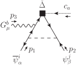
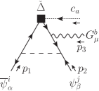
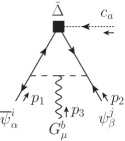
(a) Vanishing diagrams with fermion-scalar interactions.

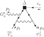
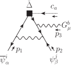
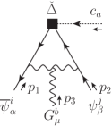
(b) Vanishing diagrams with fermion-gauge boson interactions.

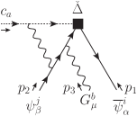
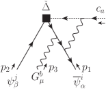
(c) Diagrams cancelling with each other.

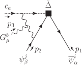
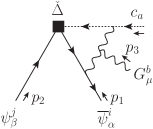
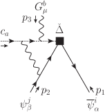
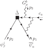
(d) The four contributing diagrams; their group structures simplify considerably when summing the first two (and last two) diagrams together.

$$i[\widecheck{\Delta}\cdot\Gamma{}_{\psi\bar{\psi}Gc}^{ji,ba,\mu}]^{(1)}_{\text{div}}=\frac{-\hbar g^{4}}{16\pi^{2}\epsilon}\frac{\xi C_{2}(G)}{8}if^{abc}{T_{R}}^{c}_{ij}\overline{\gamma}^{\mu}{\mathbb{P}_{\text{R}}}=\frac{-\hbar g^{4}}{16\pi^{2}\epsilon}\frac{\xi C_{2}(G)}{8}[{T_{R}}^{a},{T_{R}}^{b}]_{ij}\overline{\gamma}^{\mu}{\mathbb{P}_{\text{R}}}\,.$$ (6.25a)

Note that both the diagrams with the scalar propagators, and the diagrams with a gluon propagator connecting the fermions, are finite and thus do not contribute. Also, in our model there is no $$GG\Phi$$ vertex. The two diagrams with a gluon propagator connecting a fermion and the ghost leg cancel each other. The four remaining diagrams sum in pairs and their group structure simplify to get the simple result quoted above.
This 1PI Green’s function corresponds to the contribution

$$[N[\widehat{\Delta}]\cdot\Gamma_{\text{Ren}}]^{(1)}\supset\frac{-i\hbar g^{2}}{16\pi^{2}}\frac{\xi C_{2}(G)}{4}\int\operatorname{d}^{4}{x}\;ig^{2}f^{abc}{T_{R}}^{c}_{ij}c_{a}\overline{\psi}_{i}\not{G}^{b}{\mathbb{P}_{\text{R}}}\psi_{j}\,.$$ (6.25b)

$\widecheck{\Delta}c^{a}\Phi^{m}\overline{\psi^{C}}_{i,\alpha}\psi_{j,\beta}$:

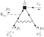
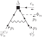
(e) Vanishing diagrams with fermion-scalar interactions.

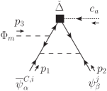
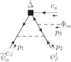
(f) Vanishing diagrams with fermion-gauge boson interactions.

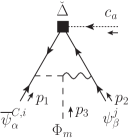
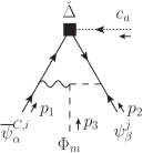
(g) Vanishing diagrams with fermion-gauge boson + fermion-scalar interactions.

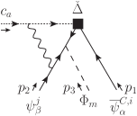
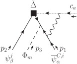
(h) Diagrams cancelling with each other.

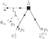
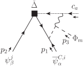
(i) The two contributing diagrams.

$$i[\widecheck{\Delta}\cdot\Gamma{}_{\psi\overline{\psi^{C}}\Phi c}^{ji,m,a}]^{(1)}_{\text{div}}=\frac{\hbar g^{3}}{16\pi^{2}\epsilon}\frac{\xi C_{2}(G)}{8}(Y_{R})^{n}_{ij}\theta^{a}_{nm}{\mathbb{P}_{\text{R}}}=\frac{\hbar g^{3}}{16\pi^{2}\epsilon}\frac{\xi C_{2}(G)}{8}({T_{\overline{R}}}^{a}Y_{R}^{m}-Y_{R}^{m}{T_{R}}^{a})_{ij}{\mathbb{P}_{\text{R}}}\,.$$ (6.26a)

Similarly to the previous case $$\widecheck{\Delta}c^{a}G^{b}_{\mu}\bar{\psi}_{i,\alpha}\psi_{j,\beta} G\Phi\Phi$$, the diagrams with scalar or gluonic propagators between the fermions, and also those with the vertex and scalar/gluon propagator between the fermions, are finite and thus do not contribute. Also, the two diagrams with a gluon propagator between a fermion and the ghost leg cancel each other. The two remaining diagrams form a pair whose total amplitude acquires a simpler group structure, after using the relation coming from the gauge-invariance of the Yukawa Lagrangian Eq. 3.14a. Thus, the 1PI Green’s function Eq. 6.26a corresponds to the contribution

$$[N[\widehat{\Delta}]\cdot\Gamma_{\text{Ren}}]^{(1)}\supset\frac{i\hbar g^{2}}{16\pi^{2}}\frac{\xi C_{2}(G)}{4}\int\operatorname{d}^{4}{x}\;\frac{g}{2}(Y_{R})^{n}_{ij}\theta^{a}_{nm}c_{a}\Phi^{m}\overline{\psi^{C}}_{i}{\mathbb{P}_{\text{R}}}\psi_{j}\,.$$ (6.26b)

Associated with this term is the complex conjugate process $$\widecheck{\Delta}c^{a}\Phi^{m}\overline{\psi}_{i,\alpha}\psi^{C}_{j,\beta}$$ that generates a similar contribution to the Bonneau identity:

$$[N[\widehat{\Delta}]\cdot\Gamma_{\text{Ren}}]^{(1)}\supset\frac{i\hbar g^{2}}{16\pi^{2}}\frac{\xi C_{2}(G)}{4}\int\operatorname{d}^{4}{x}\;\frac{g}{2}(Y_{R})^{n\;*}_{ij}\theta^{a}_{nm}c_{a}\Phi^{m}\overline{\psi}_{i}{\mathbb{P}_{\text{L}}}\psi^{C}_{j}\,.$$ (6.26c)

6.2.2 1-loop vertices with insertion of one BRST-source-vertex and $\widecheck{\Delta}$

At one-loop, and up to mass-dimension 4, the only 1PI diagrams containing a single insertion of $\widecheck{\Delta}$ and one BRST-source-vertex are those that only have one insertion of $\bar{R}s_{d}{\psi}$ or $Rs_{d}{\overline{\psi}}$ BRST-source-vertex; these diagrams have mass-dimension four. The reasons are as follows.

These diagrams should also have ghost number one since these are constituents of the Slavnov-Taylor identity. The restriction on their mass-dimensions imposes that the sum of the mass-dimensions of their incoming and outgoing fields and derivatives, has to be smaller than or equal to four. The BRST sources appear only as external fields and cannot be enclosed into loops, and their mass-dimensions are large (see Table 1). Furthermore, both the operator $\widecheck{\Delta}$ and any of the BRST-source-vertices contain only ghost fields, therefore all ghost lines from $\widecheck{\Delta}$ and any of the BRST-source-vertices give rise to an external ghost line. Thus the mass-dimension and the ghost number constraints allow only the following operators: $\rho Gcc$, $\rho\partial cc$, $\zeta ccc$, $\bar{R}\psi cc$, $R\overline{\psi}cc$ and $\mathcal{Y}\Phi cc$. The operators $\rho Gcc$, $\rho\partial cc$, $\zeta ccc$ and $\mathcal{Y}\Phi cc$ imply that the fermions from $\widecheck{\Delta}$ are enclosed into a loop, in which case one cannot form at one-loop level a 1PI diagram with the BRST-source-vertex. The remaining operators $\bar{R}\psi cc$ and $R\overline{\psi}cc$ may arise from one-loop contributions if one of the fermions of $\widecheck{\Delta}$ is contracted with a fermion from one of the operators $\bar{R}s_{d}{\psi}$ or $Rs_{d}{\overline{\psi}}$.

Only the following diagrams are therefore generated:
$\widecheck{\Delta}c^{a}c^{b}\bar{R}_{i,\alpha}\psi_{j,\beta}$:

$+(p_{2},a)\leftrightarrow(p_{3},b)$ permutation.

$$i[\widecheck{\Delta}\cdot\Gamma{}_{\psi\bar{R}cc}^{ji,ba}]^{(1)}_{\text{div}}=\frac{-i\hbar g^{4}}{16\pi^{2}\epsilon}\frac{\xi C_{2}(G)}{8}if^{abc}{T_{R}}^{c}_{ij}{\mathbb{P}_{\text{R}}}=\frac{-i\hbar g^{4}}{16\pi^{2}\epsilon}\frac{\xi C_{2}(G)}{8}[{T_{R}}^{a},{T_{R}}^{b}]_{ij}{\mathbb{P}_{\text{R}}}\,,$$ (6.27a)

corresponding to the contribution

$$[N[\widehat{\Delta}]\cdot\Gamma_{\text{Ren}}]^{(1)}\supset\frac{\hbar g^{2}}{16\pi^{2}}\frac{\xi C_{2}(G)}{4}\int\operatorname{d}^{4}{x}\;i\frac{g^{2}}{2}f^{abc}{T_{R}}^{c}_{ij}c^{a}c^{b}\bar{R}_{i}{\mathbb{P}_{\text{R}}}\psi_{j}\,.$$ (6.27b)

$\widecheck{\Delta}c^{a}c^{b}\bar{\psi}_{i,\alpha}R_{j,\beta}$:

$+(p_{2},a)\leftrightarrow(p_{3},b)$ permutation.

$$i[\widecheck{\Delta}\cdot\Gamma{}_{R\bar{\psi}cc}^{ji,ba}]^{(1)}_{\text{div}}=\frac{i\hbar g^{4}}{16\pi^{2}\epsilon}\frac{\xi C_{2}(G)}{8}if^{abc}{T_{R}}^{c}_{ij}{\mathbb{P}_{\text{L}}}=\frac{i\hbar g^{4}}{16\pi^{2}\epsilon}\frac{\xi C_{2}(G)}{8}[{T_{R}}^{a},{T_{R}}^{b}]_{ij}{\mathbb{P}_{\text{L}}}\,,$$ (6.28a)

corresponding to the contribution

$$[N[\widehat{\Delta}]\cdot\Gamma_{\text{Ren}}]^{(1)}\supset-\frac{\hbar g^{2}}{16\pi^{2}}\frac{\xi C_{2}(G)}{4}\int\operatorname{d}^{4}{x}\;i\frac{g^{2}}{2}f^{abc}{T_{R}}^{c}_{ij}c^{a}c^{b}\bar{\psi}_{i}{\mathbb{P}_{\text{L}}}R_{j}\,.$$ (6.28b)

Note that only the diagrams with a gluon propagator connecting the two ghost lines do contribute, while those where the gluon propagator connects one ghost line with a fermion line do not.

6.3 Finding the BRST-restoring finite 1-loop counterterms

In this present section we evaluate the BRST-restoring finite 1-loop counterterms $S_{\text{fct,restore}}^{(1)}$. From Eq. 6.6, we see that these finite counterterms are defined such that their 4-dimensional linear BRST transformation $b{S_{\text{fct,restore}}^{(1)}}$ cancels $[N[\widehat{\Delta}]\cdot\Gamma_{\text{Ren}}]^{(1)}$, which has been evaluated in the previous Section 6.2. We calculate these counterterms without imposing constraints on the fermion group representations and we also obtain the expression for the gauge anomalies as a by-product. These finite counterterms will be sufficient to restore the BRST invariance if the anomaly cancellation condition is met Piguet:1995er .

In order to prepare our calculations and make them easier, it is reasonable to assume that $S_{\text{fct,restore}}^{(1)}$ will be a linear combination of all possible mass-dimension $\leq 4$ field monomials whose structure can appear while calculating 1-loop Feynman diagrams. We therefore first evaluate all the linear BRST transformations of these monomials in Section 6.3.1, then we combine these results and compare them in Section 6.3.2 with the terms from $[N[\widehat{\Delta}]\cdot\Gamma_{\text{Ren}}]^{(1)}$ so as to find the finite counterterms $S_{\text{fct,restore}}^{(1)}$.

6.3.1 Evaluation of linear BRST transformation for some field monomials

The following calculations are also performed in 4 dimensions, so we will again omit all the “overlines” over all the Lorentz covariants so as to simplify the notation. The notations for the integrated field monomials are the same as in Eq. 3.36a (Section 3.2), but now all defined purely in 4 dimensions. We obtain:

$$b\int\operatorname{d}^{4}{x}\;\frac{1}{2}G^{a\,\mu}\partial^{2}G^{a}_{\mu} =\int\operatorname{d}^{4}{x}\;(\partial^{\mu}c_{a}+gf^{abc}G^{b\,\mu}c_{c})\partial^{2}G^{a}_{\mu}\,,$$ (6.29)

$$bS_{GG} =b\int\operatorname{d}^{4}{x}\;\frac{1}{2}G^{a}_{\mu}(g^{\mu\nu}\partial^{2}-\partial^{\mu}\partial^{\nu})G^{a}_{\nu}=-gf^{abc}\int\operatorname{d}^{4}{x}\;c^{a}G^{b}_{\mu}(g^{\mu\nu}\partial^{2}-\partial^{\mu}\partial^{\nu})G^{c}_{\nu}\,,$$ (6.30)

where we used the fact that $(\partial_{\mu}c^{a})(g^{\mu\nu}\partial^{2}-\partial^{\mu}\partial^{\nu})G^{a}_{\nu}=0$ when using integrations by parts.

$$bS_{GGGG} =-\frac{g^{2}}{2}(f^{abe}f^{cde}+f^{ace}f^{bde})\int\operatorname{d}^{4}{x}\;c^{a}\partial_{\nu}\left(G^{b}_{\mu}G^{c\,\mu}G^{d\,\nu}\right)\,.$$ (6.31)

In this calculation, a term proportional to $\int\operatorname{d}^{4}{x}\;c^{f}G^{e}_{\mu}G^{b\,\mu}G^{c}_{\nu}G^{d\,\nu}$ actually cancels. Indeed, its prefactor is given by: $(f^{acg}f^{bdg}+f^{adg}f^{bcg})f^{aef}$, which vanishes after symmetrizing with respect to the group indices $e\leftrightarrow b$, $c\leftrightarrow d$, and the set $(e,b)\leftrightarrow(c,d)$. Also, because $\frac{-1}{4}\int\operatorname{d}^{4}{x}\;F^{a}_{\mu\nu}F^{a\,\mu\nu}=S_{GG}+S_{GGG}+S_{GGGG}$ is gauge-invariant, $b\int\operatorname{d}^{4}{x}\;F^{a}_{\mu\nu}F^{a\,\mu\nu}=0$ and we have:

$$bS_{GGG} =-bS_{GG}-bS_{GGGG}\,.$$ (6.32)

$$b(T_{R})^{abcd}\int\operatorname{d}^{4}{x}\;G^{a}_{\mu}G^{b\,\mu}G^{c}_{\nu}G^{d\,\nu}=\\ -((T_{R})^{abcd}+(T_{R})^{acbd}+(T_{R})^{adbc}+(T_{R})^{adcb})\int\operatorname{d}^{4}{x}\;c^{a}\partial_{\nu}\left(G^{b}_{\mu}G^{c\,\mu}G^{d\,\nu}\right)\,.$$ (6.33)

As before, a term proportional to $\int\operatorname{d}^{4}{x}\;c^{f}G^{e}_{\mu}G^{b\,\mu}G^{c}_{\nu}G^{d\,\nu}$ cancels. Its prefactor is given by: $((T_{R})^{abcd}+(T_{R})^{acbd}+(T_{R})^{adbc}+(T_{R})^{adcb})f^{aef}$ (using the shorthand notation $(T_{R})^{abcd}\equiv\operatorname{Tr}[{T_{R}}^{a}\cdots{T_{R}}^{d}]$), and vanishes after symmetrization with respect to the group indices $e\leftrightarrow b$, $c\leftrightarrow d$, and the set $(e,b)\leftrightarrow(c,d)$.

$$bS_{\Phi\Phi} =b\int\operatorname{d}^{4}{x}\;\frac{-1}{2}\Phi_{m}\partial^{2}\Phi_{m}=\int\operatorname{d}^{4}{x}\;ig\theta^{a}_{mn}c^{a}\Phi_{m}\partial^{2}\Phi_{n}\,,$$ (6.34)

$$bS_{\Phi GG\Phi} =-\frac{g^{2}}{2}\{\theta^{a},\theta^{b}\}_{mn}\int\operatorname{d}^{4}{x}\;(\partial^{\mu}c^{a})G^{b}_{\mu}\Phi^{m}\Phi^{n}\,,$$ (6.35)

and because $\frac{1}{2}(D_{\mu}\Phi^{m})^{2}=S_{\Phi\Phi}+S_{\Phi G\Phi}+S_{\Phi GG\Phi}$ is gauge-invariant, $b(D_{\mu}\Phi^{m})^{2}=0$ and we have:

$$bS_{\Phi G\Phi} =-bS_{\Phi\Phi}-bS_{\Phi GG\Phi}\,.$$ (6.36)

For an arbitrary group symbol $\mathcal{C}^{a}_{mn}$,

$$b\mathcal{C}^{a}_{mn}\int\operatorname{d}^{4}{x}\;(\partial^{\mu}\Phi^{m})G^{a}_{\mu}\Phi^{n}= -\mathcal{C}^{a}_{mn}\int\operatorname{d}^{4}{x}\;c^{a}(\partial^{2}\Phi^{m})\Phi^{n}$$ (6.37)

$$-\frac{1}{2}(\mathcal{C}^{a}_{mn}+\mathcal{C}^{a}_{nm})\int\operatorname{d}^{4}{x}\;c^{a}(\partial^{\mu}\Phi^{m})(\partial_{\mu}\Phi^{n})$$

$$+ig\left[if^{abc}\mathcal{C}^{c}_{nm}+\theta^{a}_{mo}(\mathcal{C}^{b}_{on}-\mathcal{C}^{b}_{no})\right]\int\operatorname{d}^{4}{x}\;c^{a}G^{b}_{\mu}\Phi^{m}(\partial^{\mu}\Phi^{n})$$

$$+\frac{ig}{2}(\theta^{a}_{mo}\mathcal{C}^{b}_{on}+\theta^{a}_{no}\mathcal{C}^{b}_{om})\int\operatorname{d}^{4}{x}\;c^{a}(\partial^{\mu}G^{b}_{\mu})\Phi^{m}\Phi^{n}\,,$$

and, for an arbitrary group symbol $\mathcal{C}^{ab}_{mn}$,

$$b\mathcal{C}^{ab}_{mn}\int\operatorname{d}^{4}{x}\;G^{a}_{\mu}G^{b\,\mu}\Phi^{m}\Phi^{n}=-\mathcal{S}^{ab}_{mn}\int\operatorname{d}^{4}{x}\;c^{a}\partial_{\mu}\left(G^{b\,\mu}\Phi^{m}\Phi^{n}\right)\,,$$ (6.38)

where $\mathcal{S}^{ab}_{mn}=(\mathcal{C}^{ab}_{mn}+\mathcal{C}^{ba}_{mn}+m\leftrightarrow n)/2$, completely symmetric by exchanges $a\leftrightarrow b$ and $m\leftrightarrow n$. In this calculation, a term proportional to the field monomial $\int\operatorname{d}^{4}{x}\;c^{a}G^{b}_{\mu}G^{d\,\mu}\Phi^{m}\Phi^{n}$ actually cancels. Indeed, its prefactor is given by: $f^{acd}\mathcal{S}^{bc}_{mn}-i\theta^{a}_{mo}\mathcal{S}^{bd}_{on}$, and one can show that its contraction with the field monomial vanishes after symmetrizing with respect to the group indices $(b,d)$ and $(m,n)$.

We explicitly evaluate in addition the following 4-dimensional linear BRST transformations of the following fermionic operators, as these are the ones being involved in the definition of the finite counterterm action, which is naturally defined in 4 dimensions. (Note that if we were interested in their $d$-dimensional version, these would contain extra evanescent contributions.)

$$bS_{\overline{\psi}\psi}=\; b\int\operatorname{d}^{4}{x}\;i\overline{\psi}_{i}\not{\partial}\psi_{i}=g{T_{R}}^{a}_{ij}\int\operatorname{d}^{4}{x}\;c^{a}\partial_{\mu}\left(\overline{\psi}_{i}\gamma^{\mu}{\mathbb{P}_{\text{R}}}\psi_{j}\right)\,,$$ (6.39)

$$\begin{split}b(S_{\bar{R}c\psi_{R}}+S_{Rc\overline{\psi_{R}}})=\;&+i\frac{g}{2}\theta^{a}_{nm}\int\operatorname{d}^{4}{x}\;c^{a}\Phi^{m}\left((Y_{R})^{n}_{ij}\overline{\psi}^{C}_{i}{\mathbb{P}_{\text{R}}}\psi_{j}+(Y_{R})^{n\;*}_{ij}\overline{\psi}_{i}{\mathbb{P}_{\text{L}}}\psi^{C}_{j}\right)\\ &+i\frac{g^{2}}{2}f^{abc}{T_{R}}^{c}_{ij}\int\operatorname{d}^{4}{x}\;c^{a}c^{b}\left(\bar{R}^{i}{\mathbb{P}_{\text{R}}}\psi_{j}-\overline{\psi}_{i}{\mathbb{P}_{\text{L}}}R^{j}\right)\\ &+g^{2}f^{abc}{T_{R}}^{c}_{ij}\int\operatorname{d}^{4}{x}\;c^{a}\overline{\psi}_{i}\not{G}^{a}{\mathbb{P}_{\text{R}}}\psi_{j}\\ &+g{T_{R}}^{a}_{ij}\int\operatorname{d}^{4}{x}\;c^{a}\partial_{\mu}\left(\overline{\psi}_{i}\gamma^{\mu}{\mathbb{P}_{\text{R}}}\psi_{j}\right)\,.\end{split}$$ (6.40)

6.3.2 Grouping all results together – The Finite One-Loop Counterterms

The total contribution of $\widecheck{\Delta}c^{a}G^{b}_{\mu}+\widecheck{\Delta}c^{a}G^{b}_{\mu}G^{c}_{\nu}+\widecheck{\Delta}c^{a}G^{b}_{\mu}G^{c}_{\nu}G^{d}_{\rho}$ Eqs. 6.17b, 6.18b and 6.21 is equal to:

$$-\frac{\hbar g^{2}}{16\pi^{2}}\left\{\frac{S_{2}(R)}{6}b\left(5S_{GG}+S_{GGG}-\int\operatorname{d}^{4}{x}\;G^{a\,\mu}\partial^{2}G^{a}_{\mu}\right)+\frac{g^{2}}{12}(T_{R})^{abcd}b\int\operatorname{d}^{4}{x}\;G^{a}_{\mu}G^{b\,\mu}G^{c}_{\nu}G^{d\,\nu}\right\}\,,$$ (6.41)

together with relevant anomalies

$$-\frac{\hbar g^{2}}{16\pi^{2}}\left(\frac{S_{2}(R)}{3}d_{R}^{abc}\int\operatorname{d}^{4}{x}\;g\epsilon^{\mu\nu\rho\sigma}c_{a}(\partial_{\rho}G^{b}_{\mu})(\partial_{\sigma}G^{c}_{\nu})+\frac{\mathcal{D}_{R}^{abcd}}{3\times 3!}\int\operatorname{d}^{4}{x}\;g^{2}c_{a}\epsilon^{\mu\nu\rho\sigma}\partial_{\sigma}\left(G^{b}_{\mu}G^{c}_{\nu}G^{d}_{\rho}\right)\right)\,.$$ (6.42)

The contribution of $\widecheck{\Delta}c^{a}\Phi^{m}\Phi^{n}$ Eq. 6.22b is equal to:

$$-\frac{\hbar}{16\pi^{2}}\frac{Y_{2}(S)}{3}b{\overline{S_{\Phi\Phi}}}\,.$$ (6.43)

The contribution of $\widecheck{\Delta}c^{a}G^{b}_{\mu}\Phi^{m}\Phi^{n}$ Eq. 6.23b is equal to:

$$\frac{\hbar}{16\pi^{2}}\frac{(\mathcal{C}_{R})^{ab}_{mn}}{3}b\int\operatorname{d}^{4}{x}\;\frac{g^{2}}{2}G^{a}_{\mu}G^{b\,\mu}\Phi^{m}\Phi^{n}\,,$$ (6.44)

with $(\mathcal{C}_{R})^{ab}_{mn}\equiv\operatorname{Tr}\left[2\{{T_{R}}^{a},{T_{R}}^{b}\}(Y_{R}^{m})^{*}Y_{R}^{n}-{T_{R}}^{a}(Y_{R}^{m})^{*}{T_{\overline{R}}}^{b}Y_{R}^{n}\right]$.

The total contribution of $\widecheck{\Delta}c^{a}\bar{\psi}_{i,\alpha}\psi_{j,\beta}+\widecheck{\Delta}c^{a}G^{b}_{\mu}\bar{\psi}_{i,\alpha}\psi_{j,\beta}+\widecheck{\Delta}c^{a}\Phi^{m}\overline{\psi^{C}}_{i,\alpha}\psi_{j,\beta}+\widecheck{\Delta}c^{a}\Phi^{m}\overline{\psi}_{i,\alpha}\psi^{C}_{j,\beta}$
$+\widecheck{\Delta}c^{a}c^{b}\bar{R}_{i,\alpha}\psi_{j,\beta}+\widecheck{\Delta}c^{a}c^{b}\bar{\psi}_{i,\alpha}R_{j,\beta}$ Eqs. 6.24b, 6.25b, 6.26b, 6.26c, 6.27b and 6.28b is equal to:

$$\frac{-\hbar g^{2}}{16\pi^{2}}\left(1+\frac{\xi-1}{6}\right)C_{2}(R)b{S_{\overline{\psi}\psi}}+\frac{\hbar}{16\pi^{2}}\frac{\left((Y_{R}^{m})^{*}{T_{\overline{R}}}^{a}Y_{R}^{m}\right)_{ij}}{2}b\int\operatorname{d}^{4}{x}\;g\overline{\psi}_{i}\not{G}^{a}{\mathbb{P}_{\text{R}}}\psi_{j}\\ +\frac{\hbar g^{2}}{16\pi^{2}}\frac{\xi C_{2}(G)}{4}b{(S_{\bar{R}c\psi_{R}}+S_{Rc\overline{\psi_{R}}})}\,.$$ (6.45)

All in all, the BRST-restoring finite counterterms defined in 4 dimensions such as $bS_{\text{fct,restore}}^{(1)}$ cancels the contributions from $[N[\widehat{\Delta}]\cdot\Gamma_{\text{Ren}}]^{(1)}$, are:

$$\begin{split}S_{\text{fct,restore}}^{(1)}=\;&\frac{\hbar}{16\pi^{2}}\left\{g^{2}\frac{S_{2}(R)}{6}\left(5S_{GG}+S_{GGG}-\int\operatorname{d}^{4}{x}\;G^{a\,\mu}\partial^{2}G^{a}_{\mu}\right)+\frac{Y_{2}(S)}{3}\overline{S_{\Phi\Phi}}\right.\\ &\left.+g^{2}\frac{(T_{R})^{abcd}}{3}\int\operatorname{d}^{4}{x}\;\frac{g^{2}}{4}G^{a}_{\mu}G^{b\,\mu}G^{c}_{\nu}G^{d\,\nu}-\frac{(\mathcal{C}_{R})^{ab}_{mn}}{3}\int\operatorname{d}^{4}{x}\;\frac{g^{2}}{2}G^{a}_{\mu}G^{b\,\mu}\Phi^{m}\Phi^{n}\right.\\ &\left.+g^{2}\left(1+\frac{\xi-1}{6}\right)C_{2}(R)S_{\overline{\psi}\psi}-\frac{\left((Y_{R}^{m})^{*}{T_{\overline{R}}}^{a}Y_{R}^{m}\right)_{ij}}{2}\int\operatorname{d}^{4}{x}\;g\overline{\psi}_{i}\not{G}^{a}{\mathbb{P}_{\text{R}}}\psi_{j}\right.\\ &\left.-g^{2}\frac{\xi C_{2}(G)}{4}(S_{\bar{R}c\psi_{R}}+S_{Rc\overline{\psi_{R}}})\right\}\,,\end{split}$$ (6.46)

with $(\mathcal{C}_{R})^{ab}_{mn}\equiv\operatorname{Tr}\left[2\{{T_{R}}^{a},{T_{R}}^{b}\}(Y_{R}^{m})^{*}Y_{R}^{n}-{T_{R}}^{a}(Y_{R}^{m})^{*}{T_{\overline{R}}}^{b}Y_{R}^{n}\right]$, and the relevant (non-spurious) anomalies are:

$$-\frac{\hbar g^{2}}{16\pi^{2}}\left(\frac{S_{2}(R)}{3}d_{R}^{abc}\int\operatorname{d}^{4}{x}\;g\epsilon^{\mu\nu\rho\sigma}c_{a}(\partial_{\rho}G^{b}_{\mu})(\partial_{\sigma}G^{c}_{\nu})+\frac{\mathcal{D}_{R}^{abcd}}{3\times 3!}\int\operatorname{d}^{4}{x}\;g^{2}c_{a}\epsilon^{\mu\nu\rho\sigma}\partial_{\sigma}\left(G^{b}_{\mu}G^{c}_{\nu}G^{d}_{\rho}\right)\right)\,,$$ (6.47)

with the fully symmetric symbol $d_{R}^{abc}=\operatorname{Tr}[{T_{R}}^{a}\{{T_{R}}^{b},{T_{R}}^{c}\}]$, and the fully antisymmetric symbol $\mathcal{D}_{R}^{abcd}=(-i)3!\operatorname{Tr}[{T_{R}}^{a}{T_{R}}^{[b}{T_{R}}^{c}{T_{R}}^{d]}]$ for the R-representation. In realistic renormalizable models, the fermionic content and the associated group representations are chosen so as to cancel these anomalies, i.e. by cancelling separately both $\sum_{R}S_{2}(R)d_{R}^{abc}$ (proportional to the usual triangle anomaly) and $\sum_{R}\mathcal{D}_{R}^{abcd}$.

This equation Eq. 6.46 thus represents the main result of this paper. If the anomalies Eq. 6.47 are canceled, these finite counterterms are necessary and sufficient to restore the BRST symmetry at 1-loop level in the BMHV scheme. They are necessary building blocks for a consistent 1-loop applications of the scheme, and they are vital ingredients in two-loop and higher-loop order calculations. It should be noted that these finite counterterms, purely 4-dimensional and non-evanescent, are not gauge-invariant! They modify all the self-energies, as well as some specific interactions: the gauge-boson self-interactions, and the interactions between gauge-boson and scalars or fermions.

As previously mentioned in the remarks around Eq. 6.4, one can also add, to these BRST-restoring finite counterterms, any other finite counterterms that are BRST-invariant, or even that are evanescent (because they will nonetheless vanish after taking the $\mathop{\text{LIM}}_{d\to 4}$), when being defined in $d$ dimensions. However, both of these will not contribute to BRST restoration; they will instead only correspond to a change of renormalization prescription for higher-order calculations, see discussion below Eq. 4.4 in Section 4. For example, the BRST-invariant finite counterterms could contain a linear combination of the $L_{\varphi}$ functionals defined in Eqs. 4.7 and 4.8.

7 The Renormalization Group Equation in the Renormalized Model

In the present and the subsequent sections, we present the derivation of the renormalization group equation in the BMHV scheme. We focus particularly on the role of the extra counterterms specific to this scheme. Since the result will be equal to the known one, this serves as a check of the procedure and as an explanation how the additional counterterms can be treated. The present section uses methods from the abstract framework of algebraic renormalization theory, while the subsequent section proceeds in the more familiar way using renormalization constants. In both cases, we see that evanescent contributions play no role at the 1-loop level but will have an influence at higher orders. Hence, these sections provide important background information for future multi-loop applications.

As we have shown in the previous sections, the set of operators in the tree-level action is not the same set that exists at the one-loop level when using the BMHV dimensional renormalization scheme. Due to the presence of evanescent operators and finite non-evanescent counterterms needed to restore the BRST symmetry, the formalism of multiplicative renormalization (with bare fields, bare coupling constants and $Z$-factors) will not straightforwardly lead to the true renormalization group equation, that involves only fields and parameters of the original 4-dimensional tree-level action (see also discussion in Ref. Martin:1999cc ). This will be briefly overviewed in Section 8.

Instead if we start with the dimensionally renormalized 1PI functional $\Gamma_{\text{Ren}}$, see Eq. 5.8, and we use the Quantum Action Principle and the Bonneau identities, the formalism of bare objects and $Z$-factors can be avoided. From now on we take this effective action to be anomaly free, i.e. the anomalies described by Eq. 6.47 are cancelled.

7.1 Basis of Insertions

In the context of the algebraic renormalization framework, it can be shown Piguet:1995er that the renormalization group equation corresponds to the expansion of the operator insertion

$$\mu\frac{\partial}{\partial\mu}\Gamma_{\text{Ren}}=\mathcal{O}\cdot\Gamma_{\text{Ren}}$$ (7.1)

in a suitable basis of operators of ultraviolet dimension 4, ghost number 0, with contracted Lorentz indices but free gauge indices (later contracted with group factors from the associated coefficients). The basis is compounded of operators that respect the same symmetries as the functional $\mu{\partial\Gamma_{\text{Ren}}}/{\partial\mu}$, and they are, generally speaking, operators comprising derivatives with respect to the parameters of the theory, and field-counting operators,

$$\mu\frac{\partial\Gamma_{\text{Ren}}}{\partial\mu}=\Big{(}-\sum_{g}\beta_{g}\frac{\partial}{\partial g}+\sum_{\phi}\gamma_{\phi}N_{\phi}\Big{)}\Gamma_{\text{Ren}}\,.$$ (7.2)

As we will see in Section 7.2, evaluating (7.1) and (7.2) independently will result in a system of equations, overdetermined and solvable by direct comparison of their coefficients.

Let us now specialize these generally valid facts to the model discussed in our paper. Our basis will have the same symmetries as $\Gamma_{\text{Ren}}$, so it should respect the following equations Piguet:1995er :

$$\mu\frac{\partial\mathcal{S}(\Gamma_{\text{Ren}})}{\partial\mu} =\mathcal{S}_{\Gamma_{\text{Ren}}}\,\mu\frac{\partial\Gamma_{\text{Ren}}}{\partial\mu}=0\,, \frac{\delta}{\delta B}\,\mu\frac{\partial\Gamma_{\text{Ren}}}{\partial\mu} =0\,, \mathcal{G}\,\mu\frac{\partial\Gamma_{\text{Ren}}}{\partial\mu} =0\,,$$ (7.3)

i.e. respectively the BRST equation, the gauge-fixing condition and the ghost equation Piguet:1995er (with $\mathcal{G}\equiv{\delta}/{\delta\bar{c}_{a}}+\partial^{\mu}{\delta}/{\delta\rho_{a}^{\mu}}\equiv{\delta}/{\delta\widetilde{\rho}_{a}^{\mu}}$), and where

$$\begin{split}&\mathcal{S}_{\Gamma_{\text{Ren}}}=\int\operatorname{d}^{4}{x}\;\left(\frac{\delta\Gamma_{\text{Ren}}}{\delta\rho_{a}^{\mu}}\frac{\delta}{\delta G^{a}_{\mu}}+\frac{\delta\Gamma_{\text{Ren}}}{\delta G^{a}_{\mu}}\frac{\delta}{\delta\rho_{a}^{\mu}}+\frac{\delta\Gamma_{\text{Ren}}}{\delta\zeta_{a}}\frac{\delta}{\delta c^{a}}+\frac{\delta\Gamma_{\text{Ren}}}{\delta c^{a}}\frac{\delta}{\delta\zeta_{a}}+B^{a}\frac{\delta\Gamma_{\text{Ren}}}{\delta\bar{c}_{a}}\right.\\ &\left.+\frac{\delta\Gamma_{\text{Ren}}}{\delta\mathcal{Y}^{m}}\frac{\delta}{\delta\Phi_{m}}+\frac{\delta\Gamma_{\text{Ren}}}{\delta\Phi_{m}}\frac{\delta}{\delta\mathcal{Y}^{m}}+\frac{\delta\Gamma_{\text{Ren}}}{\delta\bar{R}^{i}}\frac{\delta}{\delta\psi_{i}}+\frac{\delta\Gamma_{\text{Ren}}}{\delta\psi_{i}}\frac{\delta}{\delta\bar{R}^{i}}+\frac{\delta\Gamma_{\text{Ren}}}{\delta R^{i}}\frac{\delta}{\delta\overline{\psi}_{i}}+\frac{\delta\Gamma_{\text{Ren}}}{\delta\overline{\psi}_{i}}\frac{\delta}{\delta R^{i}}\right)\,,\end{split}$$

is the linearized BRST operator of our model. The basis that respects those equations is constructed from its classical approximation, by employing the functionals $L_{G}$, $L_{c}$, $L_{\Phi}$, $L_{\psi_{R}}$ that are $b$-invariant in 4 dimensions and whose definitions have been introduced in Section 4, Eq. 4.7. These functionals can be expressed as linear combinations of field-counting operators for $d=4$ acting on the tree-level action: $L_{\varphi}\equiv\mathcal{N}_{\varphi}S_{0}$ for $\varphi=G,c,\Phi,\psi_{R}$, as well as the operators $L_{g}$, ${L_{Y_{R}}}^{m}_{ij}$ and $L_{\lambda_{mnop}}$ defined by differentiating the action with respect to the coupling parameters of the theory, Eq. 4.8.

A quantum extension of this classical basis is constructed Piguet:1995er by the action on $\Gamma_{\text{Ren}}$ of the symmetric differential operators we have just introduced (see Ref. Martin:1999cc for the details), and up to order $\hbar^{n}$ the following equation holds:

$$\Big{[}\mu\frac{\partial}{\partial\mu}+\beta\;g\frac{\partial}{\partial g}+(\beta_{Y})_{ij}^{m}\frac{\partial}{\partial Y_{ij}^{m}}+{\beta_{\lambda}}_{mnop}\frac{\partial}{\partial\lambda_{mnop}}-\gamma_{G}\mathcal{N}_{G}-\gamma_{c}\mathcal{N}_{c}-\gamma_{\Phi}\mathcal{N}_{\Phi}-\gamma_{\psi}\mathcal{N}_{\psi}^{R}\Big{]}\Gamma_{\text{Ren}}=0\,.$$ (7.4)

This is the renormalization group equation of our theory. Now, thanks to the consequence of the Quantum Action Principle that any differential operator contained in our quantum basis can be expressed as insertions of normal products in $\Gamma_{\text{Ren}}$, and the fact that the first non-vanishing contribution to these expansions is of order $\hbar$, at one-loop level we have:

$$\mu\frac{\partial\Gamma_{\text{Ren}}}{\partial\mu}\stackrel{{\scriptstyle\mathcal{O}(\hbar)}}{{=}}-\beta^{(1)}g\frac{\partial S_{0}^{(4D)}}{\partial g}-(\beta_{Y}^{(1)})_{ij}^{m}\frac{\partial S_{0}^{(4D)}}{\partial Y_{ij}^{m}}-{\beta_{\lambda}}_{mnop}^{(1)}\frac{\partial S_{0}^{(4D)}}{\partial\lambda_{mnop}}+\sum_{\phi}\gamma_{\phi}^{(1)}\mathcal{N}_{\phi}S_{0}^{(4D)}\,,$$ (7.5)

where $S_{0}^{(4D)}$ symbolizes the 4-dimensional restriction of the tree-level action of our model, Eq. 3.11. The RHS of equation (7.5) is the first constituent needed in the construction of our system of the renormalization group equations.

7.2 Evaluation of $\mu{\partial\Gamma_{\text{Ren}}}/{\partial\mu}$

The first non-trivial contribution to the functional $\mu{\partial\Gamma_{\text{Ren}}}/{\partial\mu}$ is always of order $\hbar$, since the tree-level action does not depend on the renormalization scale $\mu$. The problem of expressing $\mu{\partial\Gamma_{\text{Ren}}}/{\partial\mu}$ as an insertion of normal product operators into $\Gamma_{\text{Ren}}$ (keep in mind that $\mu$ is not a parameter of the action) was solved by Bonneau Bonneau:1980zp and generalized by Martin Martin:1999cc due to the presence of different types of fields and external sources, evanescent contributions and finite counterterms. Its restriction to one-loop ($\hbar$) order reads:

$$\mu\frac{\partial}{\partial\mu}\Gamma_{\text{Ren}}=N\big{[}\text{r.s.p.}\,\Gamma_{\text{DReg}}^{(1)}\big{]}\cdot\Gamma_{\text{Ren}}\,,$$ (7.6)

where we recall that “$\text{r.s.p.}\,\Gamma_{\text{DReg}}^{(1)}$” means the residue of the simple pole in $\nu=4-d=2\epsilon$ of all the 1PI Green’s functions described by the dimensionally-regularized effective action at $\hbar$ order, $\Gamma_{\text{DReg}}$.

Notice that, since the singular parts of Feynman diagrams contributing to 1PI Green’s functions are local polynomials in external momenta expressed in $d$, 4 and/or $\epsilon$ (i.e. evanescent) dimensions, the results generally contain evanescent contributions.

In order to handle these evanescent contributions, we will recall the results of the so-called Bonneau identities that have been first employed in Section 6.2 in the specific one-loop case, Eq. 6.14. The Bonneau identities Bonneau:1980zp ; Bonneau:1979jx form a linear system whose unique solution provides an expansion of any anomalous (e.g. evanescent) operator in terms of a quantum basis of standard insertions. More precisely, any anomalous normal product can be re-expressed as a linear combination of standard and evanescent monomial normal products Martin:1999cc , taking at any loop order the form:

$$N[\hat{g}_{\mu\nu}\mathcal{O^{\mu\nu}}](x)\cdot\Gamma_{\text{Ren}}=\sum_{i}\bar{\alpha}_{i}N[\bar{\mathcal{M}}^{i}](x)\cdot\Gamma_{\text{Ren}}+\sum_{j}\hat{\alpha}_{j}N[\hat{\mathcal{M}}^{j}](x)\cdot\Gamma_{\text{Ren}}\,,$$ (7.7)

where the $\bar{\alpha}_{i}$, $\hat{\alpha}_{j}$ coefficients are evaluated similarly to those presented in Section 6.2, Eq. 6.14, i.e. as r.s.p.’s in $4-d$ of specific 1PI Green’s functions. This engenders a $\hbar$ power expansion for these coefficients, thus showing that evanescent operators generate $\hbar$-order contributions. As shown by the latter term in Eq. 7.7, the Bonneau identities can also generate extra evanescent operators, but ponderated by additional $\hbar$-sized coefficients $\hat{\alpha}_{j}$. Such terms can be further reduced to pure standard operators by recursively applying the Bonneau identities, so that the anomalous normal product ultimately reduces to

$$N[\hat{g}_{\mu\nu}\mathcal{O^{\mu\nu}}](x)\cdot\Gamma_{\text{Ren}}=\sum_{i}q_{i}N[\bar{\mathcal{M}}^{i}](x)\cdot\Gamma_{\text{Ren}}\,,$$ (7.8)

where $q_{i}$ are formal series in $\hbar$, having no order $\hbar^{0}$ contribution due to the r.s.p. extractions on the calculations of 1PI functions entering into the definitions of the $\alpha_{i}$ coefficients. This equation (7.8) thus holds for a fixed $\hbar$ order, after reapplying a finite number of times the Bonneau identities. Fortunately, at lowest order in $\hbar$ the linear system is trivial and decoupled, i.e. loops with anomalous insertions can be transformed in sum of tree-level diagrams with insertions of standard operators.

In general, for the calculation of the coefficient $q_{i}$ at order $\hbar^{n}$, we need the coefficients $\alpha_{i}$ up to order $\hbar^{n}$ and $\hat{\alpha}_{j}$ up to order $\hbar^{n-1}$, since the evanescent operators count for an order $\hbar$ higher, according to the Bonneau identities, what is of crucial importance in particular for the calculation at one-loop level. If we now use these general results for specific operator $\mu{\partial\Gamma_{\text{Ren}}}/{\partial\mu}$, the expansion

$$\mu\frac{\partial\Gamma_{\text{Ren}}}{\partial\mu}=\sum_{i}\bar{r}_{i}N[\bar{\mathcal{W}_{i}}]\cdot\Gamma_{\text{Ren}}+\sum_{j}\hat{r}_{j}N[\hat{\mathcal{W}_{j}}]\cdot\Gamma_{\text{Ren}}$$ (7.9)

holds. Thanks to the Bonneau identities Eq. 7.8, the last term of this expansion can be re-expressed as

$$N[\hat{\mathcal{W}_{j}}]\cdot\Gamma_{\text{Ren}}=\sum_{i}c_{ji}N[\bar{\mathcal{W}_{i}}]\cdot\Gamma_{\text{Ren}}\,,$$ (7.10)

where the $c_{ji}$ are formal expansions in $\hbar$, having no order $\hbar^{0}$ contribution due to the r.s.p. extractions. This results in the expansion

$$\mu\frac{\partial\Gamma_{\text{Ren}}}{\partial\mu}=\sum_{i}r_{i}N[\bar{\mathcal{W}_{i}}]\cdot\Gamma_{\text{Ren}}\,,$$ (7.11)

and at $\hbar$ order, this equation reduces to:

$$\mu\frac{\partial\Gamma_{\text{Ren}}}{\partial\mu}=\sum_{i}r_{i}N[\bar{\mathcal{W}_{i}}]\cdot\Gamma_{\text{Ren}}=\sum_{i}(\bar{r}_{i}+{\textstyle\sum_{j}}\hat{r}_{j}c_{ji})N[\bar{\mathcal{W}_{i}}]\cdot\Gamma_{\text{Ren}}\stackrel{{\scriptstyle\mathcal{O}(\hbar)}}{{=}}\sum_{i}\bar{r}_{i}\bar{\mathcal{W}_{i}}\,,$$ (7.12)

where in the last step, the non-zero contributions at lowest $\hbar$ order come from the coefficients $\bar{r}_{i}$ only and thus, evanescent contributions do not affect one-loop level RGEs. In addition, the corresponding field product insertions $N[\bar{\mathcal{W}_{i}}]\cdot\Gamma_{\text{Ren}}$ are tree-level $\hbar^{0}$ insertions, simply equal to $\bar{\mathcal{W}_{i}}$. The general algorithm for calculating of the $\bar{r}_{i}$ and $\hat{r}_{j}$ coefficients at any order is explained in Martin:1999cc .

Now, there is a question of choice of basis for the set of 4-dimensional monomials $\bar{\mathcal{W}}_{i}$. Fortunately, any such basis of renormalized insertions is completely characterized by the corresponding classical basis Piguet:1995er . If

$$\big{\{}\Delta^{p}\cdot\Gamma=\Delta_{\text{class}}^{p}+\mathcal{O}(\hbar)\mid p=1,2,\dots;\text{dim}(\Delta^{p})\leq d\big{\}}$$ (7.13)

is the set of insertions whose classical approximations form a basis for classical insertions up to dimension $d$, then the same set is a basis for the quantum insertions bounded by $d$. This means that a convenient choice for the set of monomials are the field operators that are contained in the tree-level action $S_{0}$.

The insertion in Eq. 7.1 then can be chosen as a linear combination of operators from the 4-dimensional action,

$$\mu\frac{\partial\Gamma_{\text{Ren}}}{\partial\mu}=\sum_{i\in f.b.}\sum_{a_{i}}\overline{c}_{\phi_{1}\phi_{2}\dots}^{(1),a_{i}}\,\overline{S^{0,a_{i}}_{\phi_{1}\phi_{2}\dots}},$$ (7.14)

where $f.b.$ denotes the full basis of field operators $(\phi_{1}\phi_{2}\dots)$ in the tree-level action $S_{0}$. Thus, using our notation for Green’s functions, and in regards to Eq. 7.6 at one-loop ($\hbar$) order only, each contribution in the above equation takes the form

$$N[\text{r.s.p.}(-i)\langle\widetilde{\phi_{n}}(p_{n})\cdots\widetilde{\phi_{1}}(p_{1})\rangle^{\text{\,1PI}}{\textstyle\prod_{i}}\phi_{i}]\cdot\Gamma\\ =\text{r.s.p.}N[{\textstyle\prod_{i}}\phi_{i}\Gamma_{\phi_{n}\cdots\phi_{1}}(\bar{p}_{1},\dots,\bar{p}_{n})]\cdot\Gamma\stackrel{{\scriptstyle\mathcal{O}(\hbar)}}{{\subset}}\text{r.s.p.}(-S_{\text{sct}}^{(1),4D})\equiv-2\epsilon S_{\text{sct}}^{(1),4D}\,,$$ (7.15)

where $(1),4D$ denotes $\hbar$ order and 4-dimensional space, respectively. Therefore, at $\hbar$ order, the Renormalization Group equation acquires the simple form

$$\mu\frac{\partial\Gamma_{\text{Ren}}}{\partial\mu}\equiv-2\epsilon S_{\text{sct}}^{(1),4D}\,,$$ (7.16)

where $S_{\text{sct}}^{(1),4D}$ is just equal to Eqs. 5.31, 5.32 and 5.33 but projected onto 4 dimensions only (thus there are no appearance of evanescent operators). We again emphasize that the absence of any evanescent contribution is a one-loop effect only.

7.3 Solution of the System

By direct comparison of (7.5) with (7.16) we obtain the following system of equations:

$$S_{GG} \rightarrow 2\gamma_{G}^{(1)}=\frac{-2\hbar}{16\pi^{2}}g^{2}\frac{(13-3\xi)C_{2}(G)-4S_{2}(R)-S_{2}(S)}{6}\,,$$ (7.17)

$$S_{GGG} \rightarrow-\beta^{(1)}+3\gamma_{G}^{(1)}=\frac{-2\hbar}{16\pi^{2}}g^{2}\frac{(17-9\xi)C_{2}(G)-8S_{2}(R)-2S_{2}(S)}{12}\,,$$ (7.18)

$$S_{GGGG} \rightarrow-2\beta^{(1)}+4\gamma_{G}^{(1)}=\frac{-2\hbar}{16\pi^{2}}g^{2}\frac{2(2-3\xi)C_{2}(G)-4S_{2}(R)-S_{2}(S)}{6}\,,$$ (7.19)

$$S_{\bar{\psi}\psi_{R}} \rightarrow 2\gamma_{\psi}^{(1)}=\frac{2\hbar}{16\pi^{2}}\left(g^{2}\xi C_{2}(R)+\frac{Y_{2}(R)}{2}\right)\,,$$ (7.20)

$$S_{\overline{\psi}G\psi_{R}} \rightarrow-\beta^{(1)}+\gamma_{G}^{(1)}+2\gamma_{\psi}^{(1)}=\frac{2\hbar}{16\pi^{2}}\left(g^{2}\frac{(3+\xi)C_{2}(G)+4\xi C_{2}(R)}{4}+\frac{Y_{2}(R)}{2}\right)\,,$$ (7.21)

$$S_{\Phi\Phi} \rightarrow 2\gamma_{\Phi}^{(1)}=\frac{-2\hbar}{16\pi^{2}}\left(g^{2}(3-\xi)C_{2}(S)-Y_{2}(S)\right)\,,$$ (7.22)

$$S_{\Phi G\Phi} \rightarrow-\beta^{(1)}+\gamma_{G}^{(1)}+2\gamma_{\Phi}^{(1)}=\frac{-2\hbar}{16\pi^{2}}\left(g^{2}\left((3-\xi)C_{2}(S)-\frac{3+\xi}{4}C_{2}(G)\right)-Y_{2}(S)\right)\,,$$ (7.23)

$$S_{\Phi GG\Phi} \rightarrow-2\beta^{(1)}+2\gamma_{G}^{(1)}+2\gamma_{\Phi}^{(1)}=\frac{-2\hbar}{16\pi^{2}}\left(g^{2}\left((3-\xi)C_{2}(S)-\frac{3+\xi}{2}C_{2}(G)\right)-Y_{2}(S)\right)\,,$$ (7.24)

$$S_{\Phi^{4}_{mnop}} \rightarrow-{\beta_{\lambda}}_{mnop}^{(1)}+4\gamma^{(1)}_{\Phi}\lambda_{mnop}=\frac{-2\hbar}{16\pi^{2}}\frac{1}{2}(3g^{4}A-g^{2}\xi\Lambda^{S}-4H+\Lambda^{2})_{mnop}\,,$$ (7.25)

$$\begin{split}S_{\overline{\psi_{R}}^{C}_{i}\Phi^{m}{\psi_{R}}_{j}}&\rightarrow-(\beta_{Y}^{(1)})_{ij}^{m}+(Y_{R})^{m}_{ij}(\gamma^{(1)}_{\Phi}+2\gamma_{\psi}^{(1)})\\ &=\frac{-2\hbar}{16\pi^{2}}\left((Y_{R}^{n}(Y_{R}^{m})^{*}Y_{R}^{n})-g^{2}\frac{2C_{2}(R)(3+\xi)-C_{2}(S)(3-\xi)}{2}Y_{R}^{m}\right)_{ij}\,,\end{split}$$ (7.26)

$$S_{\bar{c}c} ,S_{\rho c}\rightarrow-\gamma_{G}^{(1)}+\gamma_{c}^{(1)}=\frac{-2\hbar}{16\pi^{2}}g^{2}\frac{3-\xi}{4}C_{2}(G)\,,$$ (7.27)

$$S_{\bar{c}Gc} ,S_{\rho Gc},S_{\zeta cc},S_{\bar{R}c\psi_{R}},S_{Rc\overline{\psi_{R}}},S_{\mathcal{Y}c\Phi}\rightarrow-\beta^{(1)}+\gamma_{c}^{(1)}=\frac{2\hbar}{16\pi^{2}}g^{2}\frac{\xi C_{2}(G)}{2}\,.$$ (7.28)

This is an overdetermined system of equations that provides the following solutions for the $\beta$-functions and anomalous dimensions at one-loop level:

$$\beta =\frac{\hbar}{16\pi^{2}}g^{2}\left(\frac{-22C_{2}(G)+4S_{2}(R)+S_{2}(S)}{6}\right)\,,$$ (7.29)

$${\beta_{\lambda}}_{mnop} =\frac{\hbar}{16\pi^{2}}(3g^{4}A_{mnop}-4H_{mnop}+\Lambda^{2}_{mnop}+\Lambda^{Y}_{mnop}-3g^{2}\Lambda^{S}_{mnop})\,,$$ (7.30)

$$\begin{split}{\beta_{Y}}_{ij}^{m}&=\frac{\hbar}{16\pi^{2}}\left(\vphantom{\frac{1}{1}}2(Y_{R}^{n}(Y_{R}^{m})^{*}Y_{R}^{n})_{ij}-3g^{2}\{C_{2}(R),Y_{R}^{m}\}_{ij}+(Y_{R})^{m}_{ij}Y_{2}(S)\right.\\ &\left.\quad+\frac{1}{2}((Y_{R})^{m}_{ij}Y_{2}(R)+Y_{2}(\bar{R})(Y_{R})^{m}_{ij})\right)\,,\end{split}$$ (7.31)

$$\gamma_{G} =\frac{\hbar}{16\pi^{2}}g^{2}\frac{(3\xi-13)C_{2}(G)+4S_{2}(R)+S_{2}(S)}{6}\,,$$ (7.32)

$$\gamma_{\psi} =\frac{\hbar}{16\pi^{2}}\frac{2g^{2}\xi C_{2}(R)+Y_{2}(R)}{2}\,,$$ (7.33)

$$\gamma_{\Phi} =\frac{\hbar}{16\pi^{2}}\left(g^{2}(\xi-3)C_{2}(S)+Y_{2}(S)\right)\,,$$ (7.34)

$$\gamma_{c} =\frac{\hbar}{16\pi^{2}}g^{2}\frac{(6\xi-22)C_{2}(G)+4S_{2}(R)+S_{2}(S)}{6}\,,$$ (7.35)

8 Comparison with the Standard Multiplicative Renormalization Approach in the BMHV Scheme

In this section, we explain the derivation of the RGE using the standard approach based on divergences of renormalization constants. In the BMHV scheme there are extra divergences for evanescent operators, and we focus particularly on their role in the derivation.

The standard textbook approach to deriving RGEs in the context of DReg was developed in Ref. tHooft:1973mfk and applied e.g. in Refs. Machacek:1983tz ; Machacek:1983fi ; Machacek:1984zw . It starts from the observation that the bare action (i.e. the sum of tree-level and counterterm action) can be written in terms of bare fields and parameters which depend on the $\overline{\text{MS}}$-renormalization scale $\mu$. For a generic bare parameter $g_{i}$ in a massless theory, and in the $\overline{\text{MS}}$-renormalization scheme, this may be written as

$$g_{i,\text{bare}} =\mu^{\rho_{i}\epsilon}\left(g_{i}+\delta g_{i}\right)\,, \delta g_{i} =\sum_{n=1}^{\infty}\frac{a_{i}^{(n)}}{\epsilon^{n}}\,,$$ (8.1)

where $\rho_{i}$ is a constant, $g_{i}$ the renormalized parameter and $\delta g_{i}$ the renormalization constant, which is a pure divergence. The coefficients $a_{i}^{(n)}$ depend on the parameters of the theory, but depend on $\mu$ only implicitly through the $\mu$-dependence of these parameters. The corresponding $\beta$ function defined as $\beta_{i}(\epsilon)\equiv{\partial g_{i}}/{\partial\ln\mu}$ is then obtained as

$$\beta_{i}(\epsilon)=-\rho_{i}\epsilon g_{i}-\rho_{i}a_{i}^{(1)}+\sum_{k}\rho_{k}g_{k}\frac{\partial a_{i}^{(1)}}{\partial g_{k}}\,,$$ (8.2)

where the sum runs over all parameters $g_{k}$ of the theory. Similarly, the anomalous dimension is obtained from the renormalization constant associated with an irreducible self-energy Green’s function, which has the expansion

$$Z_{\phi}=1+\sum_{n=1}^{\infty}\frac{a_{\phi}^{(n)}}{\epsilon^{n}}\,,$$ (8.3)

and, assuming equal renormalization of the fields in self-energy Green’s function, is equal to

$$\gamma_{\phi}(\epsilon)=\frac{1}{2}\mu\frac{d}{d\mu}\ln Z_{\phi}\,.$$ (8.4)

Proceeding similarly for all fields of the theory one obtains the generic RGE

$$\mu\frac{\partial}{\partial\mu}\Gamma_{\text{DReg}}=\Big{(}-\sum_{k}\beta_{k}(\epsilon)\frac{\partial}{\partial g_{k}}+\sum_{\phi}\gamma_{\phi}(\epsilon)N_{\phi}\Big{)}\Gamma_{\text{DReg}}\,.$$ (8.5)

This equation holds even for $\epsilon\neq 0$. An important detail is that at this level the $\beta$ and $\gamma$ functions are $\epsilon$-dependent and have the structure

$$\beta_{i}(\epsilon),\gamma_{i}(\epsilon)=\mathcal{O}(\epsilon)\times(\text{tree-level})+\mathcal{O}(\epsilon^{0})\times(\text{$\geq 1$-loop level})\,.$$ (8.6)

8.1 On the Influence of the Evanescent Counterterms

In principle, all of these remarks apply to the BMHV scheme. However, in this scheme, the action contains evanescent divergent counterterms, see Eq. 5.42. These have no tree-level counterpart. In order to apply the method in the BMHV context we can amend the tree-level action by additional terms, such that for each term in $S_{\text{sct,evan}}^{(1)}$ there is a new tree-level parameter, i.e. writing

$$S_{0,\text{amend}}=S_{0,\text{inv}}+S_{0,\text{evan}}+S_{0,\text{evan,add}}$$ (8.7)

instead of Eq. 3.35a. The parameters in the new part $S_{0,\text{evan,add}}$ will generically be denoted as $\hat{g}_{i}$. Likewise we can amend the renormalization transformation Eq. 4.1 by

$$\hat{g}_{i} \to\hat{g}_{i}+\delta\hat{g}_{i}\,.$$ (8.8)

As a result we can obtain all singular counterterms, including the evanescent ones, from a renormalization transformation, as

$$S_{0,\text{amend}}\stackrel{{\scriptstyle\text{Eqs.\ (\ref{eq:rentransform},\ref{eq:rentransformevan})}}}{{\longrightarrow}}S_{0,\text{amend}}+S_{\text{ct,inv}}+S_{\text{ct,evan}}$$ (8.9)

in place of Eq. 4.2. Via the logic described above, this leads to an RGE with the generic structure

$$\mu\frac{\partial}{\partial\mu}\Gamma_{\text{DReg}}=\Big{(}-\sum_{k}\beta_{k}(\epsilon)\frac{\partial}{\partial g_{k}}-\sum_{k}\hat{\beta}_{k}(\epsilon)\frac{\partial}{\partial\hat{g}_{k}}+\sum_{\phi}\gamma_{\phi}(\epsilon)N_{\phi}\Big{)}\Gamma_{\text{DReg}}\,,$$ (8.10)

where the second sum on the right-hand side is over all parameters $\hat{g}_{k}$ of the evanescent additional action $S_{0,\text{evan,add}}$.

In the following, we need to discuss the influence of these additional “evanescent” parameters $\hat{g}_{k}$. We first remark that such or similar parameters have been discussed in various contexts before. Ref. Schubert:1988ke considered the same problem as the present section, but in the context of a non-gauge theory, and discussed the influence of such parameters on the RGE. In the context of regularization by dimensional reduction (DRed), evanescent quantities do not correspond to $\gamma_{5}$ but to the extra $(4-d)$ degrees of freedom of the gauge fields (the so-called “$\epsilon$-scalars”). Accordingly, the impact of the $\epsilon$-scalar mass term on the 2-loop RGE of softly broken supersymmetric gauge theories has been discussed in Ref. Jack:1994rk . Finally, in applications of DRed to non-supersymmetric QCD, the evanescent coupling $\alpha_{e}$ between the $\epsilon$-scalar and quarks appears. The need for treating this coupling and its $\beta$ function as independent has been explained first in Ref. Jack:1994bn , for a further overview and references see Gnendiger:2017pys .

We now provide the following remarks:

• Our original formulation of the theory in Sections 3 to 5 corresponds to setting the evanescent parameters $\hat{g}_{k}=0$ at tree-level. This is compatible with the RGE in $\epsilon\neq 0$ only at one particular renormalization scale $\mu$. At other scales $\mu^{\prime}$, the RGE generates non-vanishing tree-level values $\hat{g}_{k}(\mu^{\prime})\neq 0$.

• Non-vanishing $\hat{g}_{i}$ enter the theory in three ways up to the 1-loop level:

  1. at tree-level in the purely evanescent part;

  2. at the 1-loop level in finite contributions to standard (non-evanescent) Green’s functions;

  3. at the 1-loop level in $1/\epsilon$ contributions to evanescent Green’s functions, and in finite contributions to $\hat{\beta}$ functions of evanescent parameters.

• Hence, applying the $\mathop{\text{LIM}}_{d\to 4}$ operation at the 1-loop level to the generic RGE (8.10), i.e. its renormalized limit, leads to:

  1. the derivative $\frac{\partial}{\partial\hat{g}_{k}}\Gamma_{\text{DReg}}$ reduces to a finite, pure 1-loop quantity;

  2. all coefficients $\beta_{k}(\epsilon)$, $\gamma_{\phi}(\epsilon)$, and $\hat{\beta}_{k}(\epsilon)$ vanish at tree-level and become quantities of 1-loop order; in the $\epsilon\to 0$ limit we denote $\beta_{k}(0)\equiv\beta_{k}\,,\,\gamma_{\phi}(0)\equiv\gamma_{\phi}\,$;

  3. the coefficients $\beta_{k}$ and $\gamma_{\phi}$ corresponding to non-evanescent operators are independent of the evanescent $\hat{g}_{k}$.

In view of these comments, the renormalized limit at the 1-loop level of Eq. 8.10 leads to the RGE

$$\mu\frac{\partial\Gamma_{\text{Ren}}}{\partial\mu}=\Big{(}-\sum_{k}\beta_{k}\frac{\partial}{\partial g_{k}}+\sum_{\phi}\gamma_{\phi}N_{\phi}\Big{)}\Gamma_{\text{Ren}}\,,$$ (8.11)

where both sides are understood to be evaluated up to the 1-loop level. The dependence on evanescent parameters $\hat{g}_{i}$ has dropped out, and the non-evanescent coefficients $\beta_{k}$, $\gamma_{\phi}$ may be evaluated by setting the $\hat{g}_{i}=0$. This shows that the correct 1-loop RGE in the BMHV context may be obtained by the simple recipe of applying the usual procedure of Refs. tHooft:1973mfk ; Machacek:1983fi from the divergences of renormalization constants, ignoring the additional evanescent objects contained in the amended tree-level action, and instead taking only the theory as defined in Sections 3 to 5.

On the other hand, this analysis also shows that starting from the 2-loop level, the situation will be more involved. E.g. the term $\hat{\beta}_{k}\frac{\partial}{\partial\hat{g}_{k}}\Gamma_{\text{DReg}}$ can be expected to provide finite, non-vanishing 2-loop contributions, and the $\beta_{i}$, $\gamma_{\phi}$ coefficients might depend on the evanescent parameters $\hat{g}_{i}$. Both effects have appeared in the contexts of Refs. Schubert:1988ke ; Schubert:1993wg ; Jack:1994rk ; Jack:1994bn mentioned above, and additional calculations are required to replace the dependence on the $\hat{g}_{i}$ by modifications of the $\beta_{i}$, $\gamma_{\phi}$.

8.2 Full system of Renormalization Group Equations

According to the previous discussion, the 1-loop RGE can be obtained from the divergences of the renormalization constants by ignoring all evanescent contributions. In this way we obtain schematically

$$\delta g^{(1)}/g \to \beta =\frac{\hbar}{16\pi^{2}}g^{2}\left(\frac{-22C_{2}(G)+4S_{2}(R)+S_{2}(S)}{6}\right)\,,$$ (8.12)

$$\delta\lambda_{mnop}^{(1)} \to {\beta_{\lambda}}_{mnop} =\frac{\hbar}{16\pi^{2}}(3g^{4}A_{mnop}-4H_{mnop}+\Lambda^{2}_{mnop}+\Lambda^{Y}_{mnop}-3g^{2}\Lambda^{S}_{mnop})\,,$$ (8.13)

$$\delta(Y_{R})^{m,(1)}_{ij} \to \begin{split}{\beta_{Y}}_{ij}^{m}&=\frac{\hbar}{16\pi^{2}}\left(\vphantom{\frac{1}{1}}2(Y_{R}^{n}(Y_{R}^{m})^{*}Y_{R}^{n})_{ij}-3g^{2}\{C_{2}(R),Y_{R}^{m}\}_{ij}+(Y_{R})^{m}_{ij}Y_{2}(S)\right.\\ &\left.\quad+\frac{1}{2}((Y_{R})^{m}_{ij}Y_{2}(R)+Y_{2}(\bar{R})(Y_{R})^{m}_{ij})\right)\,,\end{split}$$ (8.14)

$$\delta Z_{G}^{(1)} \to \gamma_{G} =\frac{\hbar}{16\pi^{2}}g^{2}\frac{(3\xi-13)C_{2}(G)+4S_{2}(R)+S_{2}(S)}{6}=-\gamma_{\bar{c}}=-\gamma_{\rho}\,,$$ (8.15)

$$\delta Z_{\psi_{L}}^{(1)} \to \gamma_{\psi} =\frac{\hbar}{16\pi^{2}}\frac{2g^{2}\xi C_{2}(R)+Y_{2}(R)}{2}=-\gamma_{R}\,,$$ (8.16)

$$\delta Z_{\Phi}^{(1)} \to \gamma_{\Phi} =\frac{\hbar}{16\pi^{2}}\left(g^{2}(\xi-3)C_{2}(S)+Y_{2}(S)\right)=-\gamma_{\mathcal{Y}}\,,$$ (8.17)

$$\delta Z_{c}^{(1)} \to \gamma_{c} =\frac{\hbar}{16\pi^{2}}g^{2}\frac{(6\xi-22)C_{2}(G)+4S_{2}(R)+S_{2}(S)}{6}=-\gamma_{\zeta}\,.$$ (8.18)

This result is the same as the one obtained in Section 7, demonstrating that both methods may be applied to obtain the correct 1-loop RGE in the BMHV scheme.

9 The Left-Handed (L) Model

In this section, we indicate how our previous results adapt for a model including only left-handed fermions. We define the Left-Handed (L) model to be the same as the Right-Handed (R) model studied so far, except now with the usage of purely left-handed fermions $\psi_{L}\equiv{\mathbb{P}_{\text{L}}}\psi$: the gauge, scalar, and gauge-scalars sectors remain unchanged, while only the fermion kinetic and Yukawa terms get modified. Our aim is to know how our results derived so far change when considering these left-handed fermions.

It is possible to construct a mapping between the L-model and the R-model: indeed, using the charge-conjugation construction from Section 2, the charge-conjugate of a left-handed fermion is a right-handed fermion:

$${\psi_{L}}^{C}=C\overline{\psi_{L}}^{T}=C(\overline{\psi}{\mathbb{P}_{\text{R}}})^{T}=C{\mathbb{P}_{\text{R}}}^{T}\overline{\psi}^{T}=C{\mathbb{P}_{\text{R}}}^{T}C^{-1}C\overline{\psi}^{T}={\mathbb{P}_{\text{R}}}C\overline{\psi}^{T}={\mathbb{P}_{\text{R}}}\psi^{C}\equiv{\mathbb{P}_{\text{R}}}\widehat{\psi}\equiv\widehat{\psi}_{R}\,,$$ (9.1)

with the definition $\widehat{\psi}\equiv\psi^{C}$.

The same discussion as in Section 3.2 holds and we can promote this L-model to $d$ dimensions. The left-handed fermion-kinetic term is:

$$\mathcal{L}_{\text{fermions}}=i\overline{\psi}_{i}\not{\partial}{\psi}_{i}+g{T_{L}}^{a}_{ij}\overline{\psi_{L}}_{i}\not{G}^{a}{\psi_{L}}_{j}\,,$$ (9.2)

where ${T_{L}}$ is the generator for their corresponding representation. Since the kinetic term is a scalar function, it is also equal to its transpose in spinor space, and thus we obtain:

$$\begin{split}\mathcal{L}_{\text{fermions}}&=i(\overline{\psi}_{i}\not{\partial}{\psi}_{i})^{T}+g{T_{L}}^{a}_{ij}(\overline{\psi_{L}}_{i}\not{G}^{a}{\psi_{L}}_{j})^{T}=-i{\psi}_{i}^{T}\overset{\leftarrow}{\not{\partial}^{T}}\overline{\psi}_{i}^{T}-g{T_{L}}^{a}_{ij}G^{a}_{\mu}{\psi_{L}}_{j}^{T}(\gamma^{\mu})^{T}\overline{\psi_{L}}_{i}^{T}\\ &=-i{\psi}_{i}^{T}C^{-1}C\overset{\leftarrow}{\not{\partial}^{T}}C^{-1}C\overline{\psi}_{i}^{T}-g{T_{L}}^{a}_{ij}G^{a}_{\mu}{\psi_{L}}_{j}^{T}C^{-1}C(\gamma^{\mu})^{T}C^{-1}C\overline{\psi_{L}}_{i}^{T}\\ &=i\overline{\psi}^{C}_{i}C\overset{\leftarrow}{\not{\partial}^{T}}C^{-1}\psi^{C}_{i}+g{T_{L}}^{a}_{ij}G^{a}_{\mu}\overline{\psi_{L}}^{C}_{j}C(\gamma^{\mu})^{T}C^{-1}{\psi_{L}}^{C}_{i}\\ &=-i\overline{\widehat{\psi}}_{i}\overset{\leftarrow}{\not{\partial}}\widehat{\psi}_{i}+g(-{T_{L}}^{a}_{ij})G^{a}_{\mu}\overline{\widehat{\psi}_{R}}_{j}\gamma^{\mu}{{}\widehat{\psi}_{R}}_{i}=i\overline{\widehat{\psi}}_{i}\not{\partial}\widehat{\psi}_{i}+g{T_{\overline{L}}}^{a}_{ij}\overline{\widehat{\psi}_{R}}_{i}\not{G}^{a}{{}\widehat{\psi}_{R}}_{j}\,,\end{split}$$ (9.3)

where in the second equality we used the anticommutativity of the fermion fields, in the second line we inserted $\mathbb{1}=C^{-1}C$ and used the properties of the charge-conjugation as defined in Section 2, and in the last line we used an integration by parts (supposing the absence of surface terms) to rewrite the pure kinetic (first) term, and defined in the interaction term ${T_{\overline{L}}}^{a}_{ij}=-{T_{L}}^{a}_{ji}$ corresponding to the complex-conjugated representation of the left-handed fermions. Posing ${T_{\widehat{R}}}^{a}_{ij}\equiv{T_{\overline{L}}}^{a}_{ij}$, we see that this conjugated $L$-representation corresponds to the representation for the associated right-handed fermions.

Let us now turn to the Yukawa term, which is a real number and therefore equals to its hermitian conjugate:

$$\begin{split}2\times\mathcal{L}_{\text{Yukawa}}=-(Y_{L})^{m}_{ij}\Phi_{m}\overline{\psi_{L}}^{C}_{i}{\psi_{L}}_{j}-(Y_{L})^{m\;*}_{ij}\Phi^{\dagger}_{m}\overline{\psi_{L}}_{i}{\psi_{L}}^{C}_{j}=-(Y_{L})^{m\;*}_{ij}\Phi^{\dagger}_{m}\overline{\widehat{\psi}_{R}}^{C}_{i}{{}\widehat{\psi}_{R}}_{j}+\text{h.c.}\,,\end{split}$$ (9.4)

and we can define $(Y_{\widehat{R}})^{m}_{ij}\equiv(Y_{L})^{m\;*}_{ij}$ the corresponding Yukawa matrix for the associated right-handed fermions, which is just the complex conjugate of the one for the left-handed fermions.

External sources for the fermion fields need to be introduced in the L-model due to the BRST quantization procedure:

$$\begin{split}S_{\bar{L}c\psi_{L}}&=\bar{L}^{i}s_{d}{\psi_{i}}=ig\bar{L}^{i}c^{a}{T_{L}}^{a}_{ij}{\psi_{L}}_{j}\equiv ig\bar{L}^{i}c^{a}{T_{L}}^{a}_{ij}{\mathbb{P}_{\text{L}}}\psi_{j}\,,\\ S_{Lc\overline{\psi_{L}}}&=s_{d}{\overline{\psi}_{i}}L^{i}=ig\overline{\psi_{L}}_{j}c^{a}{T_{L}}^{a}_{ji}L^{i}\equiv ig\overline{\psi}_{j}{\mathbb{P}_{\text{L}}}c^{a}{T_{L}}^{a}_{ji}L^{i}\,.\end{split}$$ (9.5)

Since these are scalar functions, we can take their transpose, and use the fact that $L$ and $\bar{L}$ are commuting fermions (their ghost number $=-1$) to obtain:

$$\begin{split}S_{\bar{L}c\psi_{L}}&=igc^{a}{T_{L}}^{a}_{ij}(\bar{L}^{i}{\psi_{L}}_{j})^{T}=igc^{a}{T_{L}}^{a}_{ij}{\psi_{L}}^{T}_{j}\bar{L}^{T}_{i}=igc^{a}{T_{L}}^{a}_{ij}{\psi_{L}}^{T}_{j}C^{-1}C\bar{L}^{T}_{i}\\ &=ig\overline{\psi_{L}}^{C}_{j}c^{a}(-{T_{L}}^{a}_{ij})(-C\bar{L}^{T}_{i})=ig\overline{\widehat{\psi}_{R}}_{j}c^{a}{T_{R}}^{a}_{ji}\widehat{R}_{i}\equiv S_{\widehat{R}c\overline{\widehat{\psi}_{R}}}\,,\end{split}$$ (9.6)

where we have employed the notations introduced above and have defined the external source $\widehat{R}_{i}$ for the corresponding right-handed fermions: $\widehat{R}_{i}\equiv-C\bar{L}^{T}_{i}=-{L^{C}}_{i}$. Similarly we obtain for the other source term:

$$\begin{split}S_{Lc\overline{\psi_{L}}}&=ig(\overline{\psi_{L}}_{j}L^{i})^{T}c^{a}{T_{L}}^{a}_{ji}=ig{L^{T}}^{i}\overline{\psi_{L}}^{T}_{j}c^{a}{T_{L}}^{a}_{ji}=ig{L^{T}}^{i}C^{-1}C\overline{\psi_{L}}^{T}_{j}c^{a}{T_{L}}^{a}_{ji}\\ &=ig(-{T_{L}}^{a}_{ji}){L^{T}}^{i}C^{-1}c^{a}{\psi_{L}}^{C}_{j}=ig{T_{R}}^{a}_{ij}\overline{\widehat{R}}^{i}c^{a}{{}\widehat{\psi}_{R}}_{j}\equiv S_{\overline{\widehat{R}}c\widehat{\psi}_{R}}\,,\end{split}$$ (9.7)

where we used that $\overline{\widehat{R}}_{i}=-\overline{L^{C}}_{i}=L^{T}_{i}C^{-1}$, stemming from the properties of $C$.

These calculations demonstrate that we can establish a one-to-one mapping between a left-handed model with fermions $\psi$ ($\psi_{L}\equiv{\mathbb{P}_{\text{L}}}\psi$) defined in a left-representation of the considered gauge group with generators $T_{L}$ that couple to scalar fields with the Yukawa interaction $(Y_{L})^{m}_{ij}$, and a right-handed model with fermions $\widehat{\psi}$ related via charge-conjugation: $\widehat{\psi}\equiv\psi^{C}$ ($\widehat{\psi}_{R}\equiv{\mathbb{P}_{\text{R}}}\widehat{\psi}$), in a right-representation ${T_{\widehat{R}}}^{a}_{ij}\equiv{T_{\overline{L}}}^{a}_{ij}$ that couple to the scalar fields with the Yukawa interaction $(Y_{\widehat{R}})^{m}_{ij}\equiv(Y_{L})^{m\;*}_{ij}$. Therefore, all of our calculations derived so far in this work apply to the left-handed model as well.

We are thus able to evaluate the tree-level breaking of the BRST symmetry by the action of this Left-Handed model, similarly to what has been done in Section 3.3. We find that the breaking $\widehat{\Delta}=s_{d}S_{0}$ is given by:

$$\widehat{\Delta}=\int\operatorname{d}^{d}{x}\;(g{T_{L}}^{a}_{ij})c^{a}\left\{\overline{\psi}_{i}\left(\overset{\leftarrow}{\widehat{\not{\partial}}}{\mathbb{P}_{\text{L}}}+\overset{\rightarrow}{\widehat{\not{\partial}}}{\mathbb{P}_{\text{R}}}\right)\psi_{j}\right\}\equiv\int\operatorname{d}^{d}{x}\;\widehat{\Delta}(x)\,,$$ (9.8)

generating a corresponding Feynman rule:

$$\begin{aligned} &=\frac{g}{2}{T_{L}}^{a}_{ij}\left((\widehat{\not{p_{1}}}+\widehat{\not{p_{2}}})-(\widehat{\not{p_{1}}}-\widehat{\not{p_{2}}})\gamma_{5}\right)_{\alpha\beta}\\ &=g{T_{L}}^{a}_{ij}\left(\widehat{\not{p_{1}}}{\mathbb{P}_{\text{L}}}+\widehat{\not{p_{2}}}{\mathbb{P}_{\text{R}}}\right)_{\alpha\beta}\,,\end{aligned}$$

(9.9)

and the one corresponding to the charge-conjugated fermions:

$$\widehat{\Delta}=\int\operatorname{d}^{d}{x}\;(g{T_{\overline{L}}}^{a}_{ij})c^{a}\left\{\overline{\psi^{C}}_{i}\left(\overset{\leftarrow}{\widehat{\not{\partial}}}{\mathbb{P}_{\text{R}}}+\overset{\rightarrow}{\widehat{\not{\partial}}}{\mathbb{P}_{\text{L}}}\right)\psi^{C}_{j}\right\}\,,$$ (9.10)

generating the Feynman rule:

$$\begin{aligned} &=\frac{g}{2}{T_{\overline{L}}}^{a}_{ij}\left((\widehat{\not{p_{1}}}+\widehat{\not{p_{2}}})+(\widehat{\not{p_{1}}}-\widehat{\not{p_{2}}})\gamma_{5}\right)_{\alpha\beta}\\ &=g{T_{\overline{L}}}^{a}_{ij}\left(\widehat{\not{p_{1}}}{\mathbb{P}_{\text{R}}}+\widehat{\not{p_{2}}}{\mathbb{P}_{\text{L}}}\right)_{\alpha\beta}\,.\end{aligned}$$

(9.11)

where the difference with the previous result is in the appearance of the generator ${T_{\overline{L}}}^{a}$ for the fermionic conjugate representation $L$.

The group invariants related to the scalar-fields representation $C_{2}(S),S_{2}(S),Y_{2}(S)$ and those defined in Eq. 5.23: $A_{mnop},H_{mnop},\Lambda^{2}_{mnop},\Lambda^{S}_{mnop}$ all remain the same. The group invariants $C_{2}(L),S_{2}(L),Y_{2}(L)$ of the left-representation are actually equal to those of the corresponding right-representation: $C_{2}(L)\mathbb{1}={T_{L}}^{a}{T_{L}}^{a}=(-{T_{L}}^{a\,T})(-{T_{L}}^{a\,T})={T_{\overline{L}}}^{a}{T_{\overline{L}}}^{a}=C_{2}(\overline{L})\mathbb{1}\equiv C_{2}(\widehat{R})\mathbb{1}$; $S_{2}(L)\delta^{ab}=\operatorname{Tr}({T_{L}}^{a}{T_{L}}^{b})=\operatorname{Tr}((-{T_{L}}^{b\,T})(-{T_{L}}^{a\,T}))=\operatorname{Tr}({T_{\overline{L}}}^{b}{T_{\overline{L}}}^{a})=S_{2}(\overline{L})\delta^{ab}=\operatorname{Tr}({T_{\widehat{R}}}^{a}{T_{\widehat{R}}}^{b})=S_{2}(\widehat{R})\delta^{ab}$; and $Y_{2}(L)\mathbb{1}=(Y_{L}^{m})^{*}Y_{L}^{m}=Y_{\widehat{R}}^{m}(Y_{\widehat{R}}^{m})^{*}=(Y_{\widehat{R}}^{m})^{*}Y_{\widehat{R}}^{m}\equiv Y_{2}(\widehat{R})\mathbb{1}$ by using the symmetry of the Yukawa matrices.

The singular counterterms $S_{\text{sct}}^{(1)}=S_{\text{sct}}^{(1)\,\begin{subarray}{c}\text{No Scalar}\\ \text{contrib.}\end{subarray}}+S_{\text{sct}}^{(1)\,\begin{subarray}{c}\text{Scalar}\\ \text{contrib.}\end{subarray}}$ are then obtained, and are the same as in Eqs. 5.31, 5.32 and 5.33, except for the replacements:

$$S_{2}(R)\to S_{2}(L)\,, C_{2}(R)\to C_{2}(L)\,, Y_{2}(R)\to Y_{2}(L)\,, Y_{R}^{m}\to Y_{L}^{m}\,,$$ (9.12a)

$$\overline{S_{\bar{\psi}\psi_{R}}}\to\overline{S_{\bar{\psi}\psi_{L}}}\,, \overline{S_{\overline{\psi}G\psi_{R}}}\to\overline{S_{\overline{\psi}G\psi_{L}}}\,, S_{\overline{\psi_{R}}^{C}_{i}\Phi^{m}{\psi_{R}}_{j}}\to S_{\overline{\psi_{L}}^{C}_{i}\Phi^{m}{\psi_{L}}_{j}}\,,$$ (9.12b)

$$S_{\bar{R}c\psi_{R}}\to S_{\bar{L}c\psi_{L}}\,, S_{Rc\overline{\psi_{R}}}\to S_{Lc\overline{\psi_{L}}}\,.$$ (9.12c)

Again, we can make contact to the usual renormalization transformation, and express the singular counterterms as follows:

$$S_{\text{sct}}^{(1)}=S_{\text{sct,inv}}^{(1)}+S_{\text{sct,evan}}^{(1)}\,.$$ (9.13)

The invariant counterterms $S_{\text{sct,inv}}^{(1)}$ acquire the same form as those from Eq. 4.5, in terms of the functionals $L_{\varphi}$, and with the changes:

$${\delta Z_{\psi_{R}}}\overline{L_{\psi_{R}}}\to{\delta Z_{\psi_{L}}}\overline{L_{\psi_{L}}}\,, {\delta(Y_{R})^{m}_{ij}}{L_{Y_{R}}}^{m}_{ij}\to{\delta(Y_{L})^{m}_{ij}}{L_{Y_{L}}}^{m}_{ij}\,,$$ (9.14)

and the corresponding $\delta Z_{\varphi}$, $\delta g_{i}$ renormalization constants are again the same as their counterparts Eqs. 5.35 to 5.41, but with the coefficients changed according to Eq. 9.12. The purely evanescent counterterms $S_{\text{sct,evan}}^{(1)}$ Eqs. 5.42 and 5.43 are also expressed in the same way, with the substitution $S_{2}(R)\to S_{2}(L)$.

Therefore, following the explanations given in Sections 7 and 8, the resulting renormalization group equations for the Left-handed model are the very same ones as those for the Right-handed model, with the obvious changes $R\leftrightarrow L$.

The BRST-restoring finite counterterms Eq. 6.46 now read:

$$\begin{split}S_{\text{fct,restore}}^{(1)}=\;&\frac{\hbar}{16\pi^{2}}\left\{g^{2}\frac{S_{2}(L)}{6}\left(5S_{GG}+S_{GGG}-\int\operatorname{d}^{4}{x}\;G^{a\,\mu}\partial^{2}G^{a}_{\mu}\right)+\frac{Y_{2}(S)}{3}\overline{S_{\Phi\Phi}}\right.\\ &\left.+g^{2}\frac{(T_{L})^{abcd}}{3}\int\operatorname{d}^{4}{x}\;\frac{g^{2}}{4}G^{a}_{\mu}G^{b\,\mu}G^{c}_{\nu}G^{d\,\nu}-\frac{(\mathcal{C}_{L})^{ab}_{mn}}{3}\int\operatorname{d}^{4}{x}\;\frac{g^{2}}{2}G^{a}_{\mu}G^{b\,\mu}\Phi^{m}\Phi^{n}\right.\\ &\left.+g^{2}\left(1+\frac{\xi-1}{6}\right)C_{2}(L)S_{\overline{\psi}\psi}-\frac{\left((Y_{L}^{m})^{*}{T_{\overline{L}}}^{a}Y_{L}^{m}\right)_{ij}}{2}\int\operatorname{d}^{4}{x}\;g\overline{\psi}_{i}\not{G}^{a}{\mathbb{P}_{\text{L}}}\psi_{j}\right.\\ &\left.-g^{2}\frac{\xi C_{2}(G)}{4}(S_{\bar{L}c\psi_{L}}+S_{Lc\overline{\psi_{L}}})\right\}\,,\end{split}$$ (9.15)

where we have used the following group factors:

$$\begin{split}(T_{\widehat{R}})^{a_{1}\cdots a_{n}}&=\operatorname{Tr}[{T_{\overline{L}}}^{a_{1}}\cdots{T_{\overline{L}}}^{a_{n}}]=\operatorname{Tr}\left[(-{T_{L}}^{a_{1}\,T})\cdots(-{T_{L}}^{a_{n}\,T})\right]\\ &=(-1)^{n}\operatorname{Tr}[{T_{L}}^{a_{n}}\cdots{T_{L}}^{a_{1}}]=(-1)^{n}(T_{L})^{a_{n}\cdots a_{1}}\,,\end{split}$$ (9.16a)

$$(\mathcal{C}_{L})^{ab}_{mn} \equiv\operatorname{Tr}\left[2\{{T_{L}}^{a},{T_{L}}^{b}\}(Y_{L}^{n})^{*}Y_{L}^{m}-{T_{L}}^{a}(Y_{L}^{n})^{*}{T_{\overline{L}}}^{b}Y_{L}^{m}\right]\,,$$ (9.16b)

Again, this expression is formally completely unchanged with respect to Eq. 6.46, with the only change $R\leftrightarrow L$. However, the relevant (non-spurious) anomalies Eq. 6.47 now become:

$$\boldsymbol{\boldsymbol{+}}\frac{\hbar g^{2}}{16\pi^{2}}\left(\frac{S_{2}(L)}{3}d_{L}^{abc}\int\operatorname{d}^{4}{x}\;g\epsilon^{\mu\nu\rho\sigma}c_{a}(\partial_{\rho}G^{b}_{\mu})(\partial_{\sigma}G^{c}_{\nu})+\frac{\mathcal{D}_{L}^{abcd}}{3\times 3!}\int\operatorname{d}^{4}{x}\;g^{2}c_{a}\epsilon^{\mu\nu\rho\sigma}\partial_{\sigma}\left(G^{b}_{\mu}G^{c}_{\nu}G^{d}_{\rho}\right)\right)\,,$$ (9.17)

where the group factors are the fully symmetric symbol $d_{L}^{abc}=\operatorname{Tr}[{T_{L}}^{a}\{{T_{L}}^{b},{T_{L}}^{c}\}]$ and $\mathcal{D}_{L}^{abcd}=\frac{1}{2}(d_{L}^{abe}f^{ecd}+d_{L}^{ace}f^{edb}+d_{L}^{ade}f^{ebc})$ for the L-representation. The change of sign in front of the equation, with respect to the one in Eq. 6.47, comes from the fact that these group factors for the L-representation are related to the corresponding ones in the corresponding right-handed model by: $d_{L}^{abc}=-d_{\widehat{R}}^{abc}$ and $\mathcal{D}_{L}^{abcd}=-\mathcal{D}_{\widehat{R}}^{abcd}$. This has phenomenological consequences for model-building: relevant anomalies can be cancelled in a given model if ones includes both right-handed and left-handed fermions whose representations are the complex-conjugate of the other.

10 Conclusions

The present paper starts a systematic study of the BMHV scheme for $\gamma_{5}$ and its application to chiral gauge theories such as the electroweak Standard Model. Our motivation is the increasing need for high-precision predictions including electroweak corrections at the (multi-)loop level. Many alternative $\gamma_{5}$ schemes have been proposed and used in the literature. The BMHV scheme is singled out by its mathematical rigor. It is the only scheme for which mathematical and quantum field theoretical consistency as well as useful theorems like the ones by Breitenlohner/Maison and Bonneau are fully established at all orders. Its understanding is thus not only important for practical BMHV calculations but also as a point of reference and benchmark for the study of alternative $\gamma_{5}$ schemes.

In the present paper, we have investigated a chiral gauge theory at the one-loop level. The theory includes massless chiral fermions and scalars, for simplicity restricting to irreducible representations and a simple gauge group. We have focused on the special, BMHV-specific aspects of renormalization and counterterms. Our results and conclusions can be summarized as follows.

• In Section 3 we explained in detail the setup of the BMHV scheme on the level of the $d$-dimensional tree-level action and the resulting breaking of BRST invariance (similarly to Ref. Martin:1999cc for a theory without scalars). The breaking of BRST invariance is localized in one single term, the evanescent part of the fermion kinetic term; the breaking has been expressed in a set of Feynman rules in Section 3.3.

• Section 4 provided a detailed overview of the different renormalization and counterterm structure in the BMHV scheme compared to the usual case where counterterms can be generated by a renormalization transformation. Even in the BMHV scheme, a large part of the counterterms can be generated by the usual renormalization transformation, but there are several additional, BMHV-specific new counterterm structures.

• Section 5 presented the results for the singular, i.e. UV-divergent 1-loop counterterms. Most of the counterterms follow the usual pattern and can be written in terms of field and parameter renormalization constants, see Eq. 5.34 and the following equations. However, there are extra, evanescent singular counterterms. In line with the general definitions of the BMHV scheme Breitenlohner:1975qe ; Breitenlohner:1977hr ; Breitenlohner:1975hg ; Breitenlohner:1976te as well as comparable known results in the context of dimensional reduction Gnendiger:2017pys ; Jack:1993ws ; Jack:1994bn ; Harlander:2006rj ; Harlander:2006xq ; Kilgore:2011ta ; Kilgore:2012tb ; Broggio:2015ata ; Broggio:2015dga such counterterms are necessary at higher order to ensure unitarity and finiteness. Most of the evanescent counterterms are still BRST invariant (despite being evanescent), but there are two non-BRST invariant evanescent counterterms, related to the scalar and vector self-energies, respectively.

• Section 6 corresponds to the central complication of the BMHV scheme — the breaking of gauge and BRST invariance. The breaking already present in the tree-level action implies a violation of Slavnov-Taylor identities at the 1-loop level, and special, symmetry-restoring counterterms have to be found. We have explained in detail the role and the structure of these counterterms and described various possible ways of how these counterterms may be determined. Our calculation is based on the regularized quantum action principle and the so-called Bonneau identities (this combination of tools has also been used in Ref. Martin:1999cc ); in this way, the computation is simplified to the evaluation of only UV-divergent parts of specific Feynman diagrams. While not strictly necessary at the 1-loop level, we expect that this method will lead to significant simplifications at the 2-loop level, which is why we use and explain it here in detail.

  The final result for the symmetry-restoring counterterms is given in Eq. 6.46. There is some freedom in this choice, since invariant or evanescent counterterms may be changed. Our choice is particularly simple, and is constructed to the largest possible extent from objects which appear already in the tree-level action. The terms in the symmetry-restoring counterterm action correspond to finite contributions to self-energies of scalars, fermions and gauge bosons and finite contributions to a subset of the interaction terms between scalars, fermions and gauge bosons.

• The symmetry-restoring counterterms may be changed by adding/changing evanescent terms, corresponding to defining a counterterm action $S_{\text{fct,evan}}$, see Eq. 4.4. However, all renormalized 1-loop quantities are blind to this choice, hence we do not discuss this option in the present paper. It will be relevant for a 2-loop application of the BMHV scheme, and a 2-loop calculation might be simplified by an optimized choice of $S_{\text{fct,evan}}$ at the 1-loop level.

• Section 7 and Section 8 are devoted to the derivation of the RGE in the context of the BMHV scheme. We demonstrate in two different ways that despite the extra, BMHV-specific counterterms the 1-loop RGE is unchanged compared to the familiar case of using a symmetry-invariant regularization. However, both the more abstract derivation using Bonneau identities and the textbook method based on divergent renormalization constants show that this statement relies on specific simplifications which occur at the 1-loop level. Therefore, it will be interesting and nontrivial to investigate the same situation at the 2-loop level.

As an outlook, several future extensions are of interest. First, the results can be slightly extended and specialized to the case of the electroweak SM, which has a non-semisimple gauge group, reducible representations and both right-handed and left-handed (see Section 9) chiral fermions. This is work in progress. Second, the results can be extended to higher loop orders; specifically, a knowledge of the required symmetry-restoring 2-loop counterterms will open up the possibility of 2-loop calculations in the BMHV scheme, and the determination of the 2-loop RGE will provide important information on the interpretation and the relationship between BMHV and other calculations.

References

- (1) S. L. Adler, Axial vector vertex in spinor electrodynamics, Phys. Rev. 177 (1969) 2426.
- (2) J. S. Bell and R. Jackiw, A PCAC puzzle: in the model, Nuovo Cim. A60 (1969) 47.
- (3) S. L. Adler and W. A. Bardeen, Absence of higher order corrections in the anomalous axial vector divergence equation, Phys. Rev. 182 (1969) 1517.
- (4) G. Cicuta and E. Montaldi, Analytic renormalization via continuous space dimension, Lett. Nuovo Cim. 4 (1972) 329.
- (5) C. Bollini and J. Giambiagi, Dimensional Renormalization: The Number of Dimensions as a Regularizing Parameter, Nuovo Cim. B 12 (1972) 20.
- (6) J. Ashmore, A Method of Gauge Invariant Regularization, Lett. Nuovo Cim. 4 (1972) 289.
- (7) G. ’t Hooft and M. J. G. Veltman, Regularization and Renormalization of Gauge Fields, Nucl. Phys. B44 (1972) 189.
- (8) C. Gnendiger et al., To , or not to : recent developments and comparisons of regularization schemes, Eur. Phys. J. C77 (2017) 471.
- (9) F. Jegerlehner, Facts of life with , Eur. Phys. J. C18 (2001) 673.
- (10) M. S. Chanowitz, M. Furman and I. Hinchliffe, The Axial Current in Dimensional Regularization, Nucl. Phys. B159 (1979) 225.
- (11) D. Kreimer, The Problem and Anomalies: A Clifford Algebra Approach, Phys. Lett. B237 (1990) 59.
- (12) J. G. Korner, D. Kreimer and K. Schilcher, A Practicable scheme in dimensional regularization, Z. Phys. C54 (1992) 503.
- (13) D. Kreimer, The Role of in dimensional regularization, hep-ph/9401354 UTAS-PHYS-94-01, 1993, [hep-ph/9401354].
- (14) N. Zerf, Fermion Traces Without Evanescence, Phys. Rev. D101 (2020) 036002.
- (15) D. Akyeampong and R. Delbourgo, Dimensional regularization, abnormal amplitudes and anomalies, Nuovo Cim. A 17 (1973) 578.
- (16) D. Akyeampong and R. Delbourgo, Dimensional regularization and PCAC, Nuovo Cim. A 18 (1973) 94.
- (17) D. Akyeampong and R. Delbourgo, Anomalies via dimensional regularization, Nuovo Cim. A 19 (1974) 219.
- (18) P. Breitenlohner and D. Maison, Dimensional Renormalization of Massless Yang-Mills Theories, MPI-PAE-PTH-26-75, 1975.
- (19) P. Breitenlohner and D. Maison, Dimensional Renormalization and the Action Principle, Commun. Math. Phys. 52 (1977) 11.
- (20) P. Breitenlohner and D. Maison, Dimensionally Renormalized Green’s Functions for Theories with Massless Particles. 1., Commun. Math. Phys. 52 (1977) 39.
- (21) P. Breitenlohner and D. Maison, Dimensionally Renormalized Green’s Functions for Theories with Massless Particles. 2., Commun. Math. Phys. 52 (1977) 55.
- (22) A. V. Bednyakov and A. F. Pikelner, Four-loop strong coupling beta-function in the Standard Model, Phys. Lett. B762 (2016) 151 [1508.02680].
- (23) M. F. Zoller, Top-Yukawa effects on the -function of the strong coupling in the SM at four-loop level, JHEP 02 (2016) 095.
- (24) C. Poole and A. E. Thomsen, Weyl Consistency Conditions and , Phys. Rev. Lett. 123 (2019) 041602 [1901.02749].
- (25) C. Becchi, A. Rouet and R. Stora, Renormalization of Gauge Theories, Annals Phys. 98 (1976) 287.
- (26) I. V. Tyutin, Gauge Invariance in Field Theory and Statistical Physics in Operator Formalism, 0812.0580 LEBEDEV-75-39, 1975, [0812.0580].
- (27) O. Piguet and A. Rouet, Symmetries in Perturbative Quantum Field Theory, Phys. Rept. 76 (1981) 1.
- (28) O. Piguet and S. P. Sorella, Algebraic renormalization: Perturbative renormalization, symmetries and anomalies, Lect. Notes Phys. Monogr. 28 (1995) 1.
- (29) D. Binosi and J. Papavassiliou, Pinch Technique: Theory and Applications, Phys. Rept. 479 (2009) 1.
- (30) C. P. Martin and D. Sanchez-Ruiz, Action principles, restoration of BRS symmetry and the renormalization group equation for chiral non-Abelian gauge theories in dimensional renormalization with a non-anticommuting , Nucl. Phys. B572 (2000) 387.
- (31) D. Sanchez-Ruiz, BRS symmetry restoration of chiral Abelian Higgs-Kibble theory in dimensional renormalization with a non-anticommuting , Phys. Rev. D68 (2003) 025009 [hep-th/0209023].
- (32) R. Ferrari, A. Le Yaouanc, L. Oliver and J. Raynal, Gauge invariance and dimensional regularization with in flavor changing neutral processes, Phys. Rev. D 52 (1995) 3036.
- (33) W. Hollik, E. Kraus and D. Stöckinger, Renormalization and symmetry conditions in supersymmetric QED, Eur. Phys. J. C11 (1999) 365.
- (34) P. A. Grassi, T. Hurth and M. Steinhauser, Practical algebraic renormalization, Annals Phys. 288 (2001) 197.
- (35) P. A. Grassi, T. Hurth and M. Steinhauser, The Algebraic method, Nucl. Phys. B610 (2001) 215.
- (36) I. Fischer, W. Hollik, M. Roth and D. Stöckinger, Restoration of supersymmetric Slavnov-Taylor and Ward identities in presence of soft and spontaneous symmetry breaking, Phys. Rev. D69 (2004) 015004.
- (37) A. Blondel et al., Standard model theory for the FCC-ee Tera-Z stage, in Mini Workshop on Precision EW and QCD Calculations for the FCC Studies : Methods and Techniques CERN, Geneva, Switzerland, January 12-13, 2018, vol. 3, (Geneva), CERN, CERN, 2019, 10.23731/CYRM-2019-003 [1809.01830].
- (38) A. M. Bruque, A. L. Cherchiglia and M. Pérez-Victoria, Dimensional regularization vs methods in fixed dimension with and without , JHEP 08 (2018) 109.
- (39) C. Gnendiger and A. Signer, in the four-dimensional helicity scheme, Phys. Rev. D 97 (2018) 096006 [1710.09231].
- (40) R. A. Fazio, P. Mastrolia, E. Mirabella and W. J. Torres Bobadilla, On the Four-Dimensional Formulation of Dimensionally Regulated Amplitudes, Eur. Phys. J. C74 (2014) 3197.
- (41) A. J. Buras and M. Munz, Effective Hamiltonian for beyond leading logarithms in the NDR and HV schemes, Phys. Rev. D52 (1995) 186.
- (42) S. A. Larin, The Renormalization of the axial anomaly in dimensional regularization, Phys. Lett. B303 (1993) 113.
- (43) T. L. Trueman, Spurious anomalies in dimensional renormalization, Z. Phys. C69 (1996) 525.
- (44) K. G. Chetyrkin, M. Misiak and M. Munz, nonleptonic effective Hamiltonian in a simpler scheme, Nucl. Phys. B520 (1998) 279.
- (45) C. Schubert, On the problem of dimensional renormalization, HD-THEP-93-46, 1993.
- (46) G. Bonneau, Zimmermann Identities And Renormalization Group Equation In Dimensional Renormalization, Nucl. Phys. B167 (1980) 261.
- (47) G. Bonneau, Trace and Axial Anomalies in Dimensional Renormalization Through Zimmermann Like Identities, Nucl. Phys. B171 (1980) 477.
- (48) W. Siegel, Supersymmetric Dimensional Regularization via Dimensional Reduction, Phys. Lett. 84B (1979) 193.
- (49) W. Siegel, Inconsistency of Supersymmetric Dimensional Regularization, Phys. Lett. 94B (1980) 37.
- (50) D. M. Capper, D. R. T. Jones and P. van Nieuwenhuizen, Regularization by Dimensional Reduction of Supersymmetric and Nonsupersymmetric Gauge Theories, Nucl. Phys. B167 (1980) 479.
- (51) D. Stöckinger, Regularization by dimensional reduction: consistency, quantum action principle, and supersymmetry, JHEP 03 (2005) 076.
- (52) S. P. Martin and M. T. Vaughn, Regularization dependence of running couplings in softly broken supersymmetry, Phys. Lett. B 318 (1993) 331.
- (53) L. Mihaila, Two-loop parameter relations between dimensional regularization and dimensional reduction applied to SUSY-QCD, Phys. Lett. B 681 (2009) 52.
- (54) D. Stockinger and P. Varso, FeynArts model file for MSSM transition counterterms from DREG to DRED, Comput. Phys. Commun. 183 (2012) 422 [1109.6484].
- (55) J. C. Collins, Renormalization, vol. 26 of Cambridge Monographs on Mathematical Physics. Cambridge University Press, Cambridge, 1986, 10.1017/CBO9780511622656.
- (56) T. Marinucci and M. Tonin, Dimensional Regularization and Anomalies, Nuovo Cim. A 31 (1976) 381.
- (57) P. Frampton, Conditions for Renormalizability of Quantum Flavor Dynamics, Phys. Rev. D 20 (1979) 3372.
- (58) G. Bonneau, Consistency in Dimensional Regularization With , Phys. Lett. 96B (1980) 147.
- (59) K. Hieda, A. Kasai, H. Makino and H. Suzuki, 4D SYM supercurrent in terms of the gradient flow, PTEP 2017 (2017) 063B03.
- (60) E.-C. Tsai, Gauge Invariant Treatment of in the Scheme of ’t Hooft and Veltman, Phys. Rev. D83 (2011) 025020 [0905.1550].
- (61) H. K. Dreiner, H. E. Haber and S. P. Martin, Two-component spinor techniques and Feynman rules for quantum field theory and supersymmetry, Phys. Rept. 494 (2010) 1.
- (62) M. E. Machacek and M. T. Vaughn, Two Loop Renormalization Group Equations in a General Quantum Field Theory. 1. Wave Function Renormalization, Nucl. Phys. B222 (1983) 83.
- (63) M. E. Machacek and M. T. Vaughn, Two Loop Renormalization Group Equations in a General Quantum Field Theory. 2. Yukawa Couplings, Nucl. Phys. B236 (1984) 221.
- (64) M. E. Machacek and M. T. Vaughn, Two Loop Renormalization Group Equations in a General Quantum Field Theory. 3. Scalar Quartic Couplings, Nucl. Phys. B249 (1985) 70.
- (65) T. van Ritbergen, A. N. Schellekens and J. A. M. Vermaseren, Group theory factors for Feynman diagrams, Int. J. Mod. Phys. A14 (1999) 41.
- (66) M.-x. Luo, H.-w. Wang and Y. Xiao, Two loop renormalization group equations in general gauge field theories, Phys. Rev. D67 (2003) 065019 [hep-ph/0211440].
- (67) I. Schienbein, F. Staub, T. Steudtner and K. Svirina, Revisiting RGEs for general gauge theories, Nucl. Phys. B939 (2019) 1.
- (68) S. P. Martin, TASI 2011 lectures notes: two-component fermion notation and supersymmetry, in The Dark Secrets of the Terascale: Proceedings, TASI 2011, Boulder, Colorado, USA, Jun 6 - Jul 11, 2011, pp. 199–258, 2013, 10.1142/9789814390163_0005 [1205.4076].
- (69) N. Nakanishi, Covariant Quantization of the Electromagnetic Field in the Landau Gauge, Prog. Theor. Phys. 35 (1966) 1111.
- (70) B. Lautrup, Canonical Quantum Electrodynamics In Covariant Gauges, Kong. Dan. Vid. Sel. Mat. Fys. Med. 35 (1967) .
- (71) I. A. Batalin and G. A. Vilkovisky, Relativistic S Matrix of Dynamical Systems with Boson and Fermion Constraints, Phys. Lett. 69B (1977) 309.
- (72) I. A. Batalin and G. A. Vilkovisky, Gauge Algebra and Quantization, Phys. Lett. 102B (1981) 27.
- (73) I. A. Batalin and G. A. Vilkovisky, Quantization of Gauge Theories with Linearly Dependent Generators, Phys. Rev. D28 (1983) 2567.
- (74) A. Denner, H. Eck, O. Hahn and J. Kublbeck, Feynman rules for fermion number violating interactions, Nucl. Phys. B387 (1992) 467.
- (75) A. Denner, H. Eck, O. Hahn and J. Kublbeck, Compact Feynman rules for Majorana fermions, Phys. Lett. B291 (1992) 278.
- (76) I. Jack, D. R. T. Jones and K. L. Roberts, Dimensional Reduction in Non-Supersymmetric Theories, Z. Phys. C62 (1994) 161.
- (77) I. Jack, D. R. T. Jones and K. L. Roberts, Equivalence of dimensional reduction and dimensional regularization, Z. Phys. C63 (1994) 151.
- (78) R. Harlander, P. Kant, L. Mihaila and M. Steinhauser, Dimensional Reduction applied to QCD at three loops, JHEP 09 (2006) 053.
- (79) R. V. Harlander, D. R. T. Jones, P. Kant, L. Mihaila and M. Steinhauser, Four-loop beta function and mass anomalous dimension in dimensional reduction, JHEP 12 (2006) 024.
- (80) W. B. Kilgore, Regularization Schemes and Higher Order Corrections, Phys. Rev. D83 (2011) 114005 [1102.5353].
- (81) W. B. Kilgore, The Four Dimensional Helicity Scheme Beyond One Loop, Phys. Rev. D86 (2012) 014019 [1205.4015].
- (82) A. Broggio, C. Gnendiger, A. Signer, D. Stöckinger and A. Visconti, Computation of in and : renormalization, operator mixing, and explicit two-loop results, Eur. Phys. J. C75 (2015) 418.
- (83) A. Broggio, C. Gnendiger, A. Signer, D. Stöckinger and A. Visconti, SCET approach to regularization-scheme dependence of QCD amplitudes, JHEP 01 (2016) 078.
- (84) T. Hahn, Generating Feynman diagrams and amplitudes with FeynArts 3, Comput. Phys. Commun. 140 (2001) 418.
- (85) R. Mertig, M. Bohm and A. Denner, FEYN CALC: Computer algebraic calculation of Feynman amplitudes, Comput. Phys. Commun. 64 (1991) 345.
- (86) V. Shtabovenko, R. Mertig and F. Orellana, New Developments in FeynCalc 9.0, Comput. Phys. Commun. 207 (2016) 432.
- (87) V. Shtabovenko, R. Mertig and F. Orellana, FeynCalc 9.3: New features and improvements, 2001.04407 P3H-20-002, TTP19-020, TUM-EFT 130/19, 1, 2020, [2001.04407].
- (88) V. Shtabovenko, FeynHelpers: Connecting FeynCalc to FIRE and Package-X, Comput. Phys. Commun. 218 (2017) 48.
- (89) H. H. Patel, Package-X 2.0: A Mathematica package for the analytic calculation of one-loop integrals, Comput. Phys. Commun. 218 (2017) 66 [1612.00009].
- (90) S. Weinberg, The quantum theory of fields. Vol. 2: Modern applications. Cambridge University Press, 2013.
- (91) M. E. Peskin and D. V. Schroeder, An Introduction to quantum field theory. Addison-Wesley, Reading, USA, 1995.
- (92) M. Srednicki, Quantum field theory. Cambridge University Press, 1, 2007.
- (93) W. Hollik and D. Stöckinger, Regularization and supersymmetry restoring counterterms in supersymmetric QCD, Eur. Phys. J. C20 (2001) 105.
- (94) W. Hollik and D. Stöckinger, MSSM Higgs-boson mass predictions and two-loop non-supersymmetric counterterms, Phys. Lett. B634 (2006) 63.
- (95) D. Stöckinger and J. Unger, Three-loop MSSM Higgs-boson mass predictions and regularization by dimensional reduction, Nucl. Phys. B935 (2018) 1 [1804.05619].
- (96) W. Zimmermann, Composite operators in the perturbation theory of renormalizable interactions, Annals Phys. 77 (1973) 536.
- (97) W. Zimmermann, Normal products and the short distance expansion in the perturbation theory of renormalizable interactions, Annals Phys. 77 (1973) 570.
- (98) J. H. Lowenstein, Normal product quantization of currents in Lagrangian field theory, Phys. Rev. D4 (1971) 2281.
- (99) J. C. Collins, Normal Products in Dimensional Regularization, Nucl. Phys. B92 (1975) 477.
- (100) G. ’t Hooft, Dimensional regularization and the renormalization group, Nucl. Phys. B61 (1973) 455.
- (101) C. Schubert, The Yukawa Model as an Example for Dimensional Renormalization With , Nucl. Phys. B323 (1989) 478.
- (102) I. Jack, D. R. T. Jones, S. P. Martin, M. T. Vaughn and Y. Yamada, Decoupling of the epsilon scalar mass in softly broken supersymmetry, Phys. Rev. D50 (1994) R5481.