Spin-up of a superfluid vortex lattice driven by rough boundaries

Abstract

We study numerically the formation of a vortex lattice inside a rotating bucket containing superfluid helium, paying attention to an important feature which is practically unavoidable in all experiments: the microscopic roughness of the bucket’s surface. We model this using the Gross-Pitaevskii equation for a weakly-interacting Bose gas, a model which is idealised when applied to superfluid helium but captures the key physics of the vortex dynamics which we are interested in. We find that the vortex lattice arises from the interaction and reconnections of nucleated U-shaped vortex lines, which merge and align along the axis of rotation. We quantify the effects which the surface roughness and remanent vortex lines play in this process.

I Introduction

Superfluids are extraordinary fluids characterised by the absence of viscosity. They are irrotational everywhere except at vortex lines whose circulation is quantised in units of $\kappa=h/m$, where $h$ is Planck’s constant and $m$ is the mass of the boson which composes the fluid Annett2004 ; Barenghi2016 . First discovered and studied in liquid helium-4 and, decades later, in helium-3, superfluidity has since been observed in ultracold gases and photonic systems. The constraint of quantised vorticity is a consequence of quantum mechanics - vorticity can only arise as $2\pi$ topological defects of the macroscopic single-particle wavefunction of the quantum many-body system. These defects manifest as vortex lines through the fluid. As well as possessing a circulating flow, the vortex lines have a core of depleted density about their axis, out to a core radius $a_{0}$ which is of the order of the superfluid healing length. In helium-4 and helium-3 the vortex core size is around $10^{-10}$m and $10^{-8}$m, respectively.

The textbook paradigm of superfluidity is a cylindrical bucket of superfluid helium rotating at constant angular frequency $\Omega$. Classical solid-body rotation is forbidden by the irrotational nature of the superfluid. At sufficiently small values of $\Omega$, the fluid remains quiescent. However, if $\Omega$ in increased past a critical value $\Omega_{\rm c}$, the presence of a vortex line is energetically favourable. Using hydrodynamic arguments and up to a logarithmic correction, it is estimated Barenghi2016 that this critical angular frequency is

$$\Omega_{\rm c}=\frac{\hbar}{mR^{2}}\ln\left(\frac{R}{a_{0}}\right),$$ (1)

where $m$ is the mass of a helium atom and $R$ is the radius of the bucket. At larger values of $\Omega$, two vortices become favourable, and so on. For $\Omega\gg\Omega_{\rm c}$ the stationary state of the fluid is the famed vortex lattice, an array of vortex lines aligned along the axis of rotation with areal density

$$n_{\rm v}=\frac{2\Omega}{\kappa},$$ (2)

known as Feynman’s rule. The vortex lattice was first imaged in superfluid helium by Packard et al Yarmchuk1979 and more recently by Bewley et al Bewley2006 . The lattice has also been observed in ultracold gaseous superfluids trapped by smooth confining potentials Madison2000 ; AboShaeer2001 . (At much higher rotation frequencies where centrifugal effects dominate, a giant or macroscopic vortex carrying many quanta of circulation can become formed in both superfluid helium Tsakadze1964 ; Josserand2004 and gaseous superfluids Kasamatsu2002 ; Fischer2003 ; Kavoulakis2003 ; Engels2003 ; however, this regime is outside the scope of this work.)

The process in which the vortices enter the superfluid in the first place is called vortex nucleation. Being associated with a $2\pi$ phase singularity of the macroscopic wavefunction, a vortex line is topologically protected. Thus, starting from some initially vortex-free state, vortices must enter the superfluid from the boundary. It is believed that vortex lines are nucleated either intrinsically by the flow of the superfluid past the microscopic roughness of the bucket wall (overcoming a critical velocity) or extrinsically by stretching some pre-existing vortex lines called “remanent vortices” which, under suitably conditions, can spool additional vortices Schwarz-mill . Remanent vortices are thought to arise when cooling the helium sample through the superfluid transition, and can be avoided by using careful experimental protocols Yano-2007 .

Individual vortex nucleation in a rotating bucket, either intrinsic or extrinsic, has never been visualised in detail. Experimentally, it remains challenging to image the flow in the vicinity of a boundary, despite progress in flow visualisation in the bulk Bewley2006 ; Zmeev2015b ; Duda2015 , more so because the microscopic scale of the vortices themselves. Theoretically, the nucleation problem has been addressed using energy arguments Fetter1966 ; StaufferFetter1968 with no insight in the dynamics. With few exceptions Stagg2017 , the effect of microscopic boundary roughness on the vortex nucleation has not been studied. A related and better understood nucleation process takes place when an ion bubble is driven in liquid helium by an applied electric field; compared to the bucket, the nucleation is more controlled in terms of geometry (the shape of the bubble can be determined theoretically) and velocity (experimentally determined by time of flight measurements). Vortex nucleation by the ion bubble has thus received much detailed experimental and theoretical attention MuirheadVinenDonnelly1984 ; McClintockBowley1995 ; BerloffRoberts2000 ; Winiecki2000 ; Villois2018 than nucleation by the walls of the bucket which contains the helium sample.

In this work we are not concerned with the vortex nucleation as such, but rather with the intermediate state between the nucleation and the final vortex lattice. This intermediate stage is still unexplored, but, given that the length scales and the time scales involved depend on the vortex separation rather the vortex core size (i.e. they are mesoscopic rather than microscopic), there is prospect of experimental visualisation in the near future. The focus of attention is therefore not individual vortex dynamics at nucleation but the collective dynamics of many vortex lines in the presence of a boundary which is not smooth. For simplicity we consider the problem at sufficiently low temperature that the normal fluid does not play an important role.

The traditional method to model the dynamics of superfluid vortices is the Vortex Filament Method (VFM) Schwarz1988 , which models vortex lines as infinitesimally thin filaments interacting with themselves, their neighbours and the boundary (via suitable images). However, this approach is not applicable to our problem. Firstly, if the boundary varies on atomic length scales comparable to the vortex core (which is likely to be the case for any metal or glass bucket containing liquid helium), then the core lengthscale can no longer be ignored compared to other relevant lengthscale, invalidating the assumptions behind the VFM. Secondly, the implementation of the boundary condition is cumbersome to set up and not simple to change from one boundary shape to another; indeed, the VFM has been implemented for plane Schwarz1985 , semi-spherical Schwarz1985 ; Tsubota1993 , spherical Schwarz1974 ; Kivotides2006 and cylindrical Hanninen2005 ; HanninenBaggaley2014 boundaries, but never for irregular boundaries relevant to our problem. Thirdly, the VFM does not describe vortex nucleation, but requires to initialise the calculation with arbitrary seeding vortex lines. An alternative approach is through the Gross-Pitaevskii equation (GPE) Pitaevskii ; Barenghi2016 . This is a formal description of a dilute weakly-interacting gas of bosons, and is equivalent to a continuity equation and an Euler-like equation for an inviscid fluid (the modification being the presence of a quantum pressure term). While the GPE is an excellent quantitative description of Bose gas superfluids, it is limited to being a qualitative description of superfluid helium due to the stronger interactions taking place in a liquid rather than in a gas. Nevertheless, its capability to describe the microscopic detail of superfluid dynamics - the finite-sized core, vortex interactions and reconnections, even the intrinsic nucleation - makes it a useful model to study superfluid flows at a boundary. An important feature is that the GPE can easily implement irregular boundaries. Indeed, recent GPE simulations have predicted the occurrence of a turbulent boundary layer when the superfluid flows past a locally rough surface Stagg2017 : above a critical imposed flow speed, vortices are nucleated from the surface features, interact and become entwined in a layer adjacent to the surface.

Returning to the rotating bucket of superfluid helium, it is natural to ask if some kind of boundary layer may similarly form at the boundary of the rotating bucket in the transient evolution to the vortex lattice. Whether disordered or laminar, this layer will certainly involve vortex interactions. It is in fact unlikely that the vortex lines which nucleate extend from the top to the bottom of the bucket, as if the process were essentially two-dimensional (2D). More likely, the first vortex lines which nucleate are small, and become long only after a sequence of interactions and reconnections. To qualitatively explore these interactions, here we perform a series of numerical experiments, based on the GPE, of a superfluid being spun-up in a bucket whose walls are microscopically rough. These numerical experiments allows us to build a physical picture of how vorticity enters the superfluid and forms a vortex lattice, and of the role of remanent vortices, sharp intrusions, rotation rate, and dimensionality.

The plan of the paper is the following. In Section II we introduce our model and details our of numerical simulations. In Section III we present our main results for the spin up of a quiescent superfluid. Section IV explores the possibility that a single strong imperfection in the shape of a protuberance, remanent vortex lines or dimensionality may affect the main results described in Section III. Finally, in Section V we discuss and conclude our findings.

II Model and method

II.1 Gross-Pitaevskii equation

We model the superfluid dynamics using the Gross-Pitaevskii equation. Within this model, the superfluid is parametrised by a mean-field complex wavefunction $\Psi({\bf r},t)=|\Psi({\bf r},t)|e^{iS(\bf r,t)}$. The particle density follows as $n({\bf r},t)=|\Psi({\bf r},t)|^{2}$ and the fluid velocity as ${\bf v}({\bf r},t)=(\hbar/m)\nabla S({\bf r},t)$, where $\hbar=h/(2\pi)$ and $S({\bf r},t)$ is the phase distribution of $\Psi$. The dynamics of $\Psi({\bf r},t)$ follows the GPE Pitaevskii ; Barenghi2016 ,

$$i\hbar\frac{\partial\Psi}{\partial t}=\hat{\mathcal{H}}\Psi,$$ (3)

with Hamiltonian operator,

$$\hat{\mathcal{H}}=-\frac{\hbar^{2}}{2m}\nabla^{2}+V+g\left|\Psi\right|^{2}.$$ (4)

Here $m$ is the particle mass, $g$ $(>0)$ is a nonlinear coefficient describing the inter-particle interactions, and $V({\bf r},t)$ is the external potential acting on the fluid. Stationary solutions of the GPE satisfy $\hat{\mathcal{H}}\Psi=\mu_{0}\Psi$, where $\mu_{0}$ is the chemical potential of the fluid.

We make two physically-motivated modifications to the basic GPE above. Firstly, since the GPE conserves energy, we follow other works Choi1998 ; Tsubota2001 in introducing a phenomenological dissipation term into the GPE to model, at least in a qualitative way, the damping of excitations of the superfluid (for example, by their interaction with the normal fluid). This is achieved by replacing the left-side of Eq. (3) with $(i-\gamma)\hbar\,\partial\Psi/\partial t$, where $\gamma$ specifies the strength of the dissipation. Although not as accurate the friction included within the VFM, this phenomenological dissipation will help damp out the oscillations of the vortex lines (Kelvin waves), which is the main effect of the friction which concerns us here. Secondly, given our rotating scenario, we work in the reference frame rotating at constant angular frequency $\Omega$ about the $z$ axis; this is achieved by modifying the GPE Hamiltonian to $\hat{\mathcal{H}}-i\Omega L_{z}$, where $L_{z}$ is the angular momentum operator about $z$. In Cartesian coordinates $L_{z}=i\hbar(y\partial_{x}-x\partial_{y})$.

II.2 Bucket set-up

We consider the fluid to be confined within a cylindrical bucket of radius $R$ and height $H$. The axis of the cylinder is the z-axis of rotation. The bucket is modelled through the potential $V({\bf r})$: in the interior of the bucket we set $V=0$ while at the boundary and beyond we set $V\gg\mu_{0}$. In the ground state, the fluid density has the bulk value $n_{0}$ in the centre of the bucket, while close to the bucket wall it heals to zero density over a length scale characterised by the healing length $\xi=\hbar/\sqrt{mn_{0}g}$. The healing length also characterises the size of the cores of vortices in the fluid. Note that the chemical potential in the bulk is $\mu_{0}=n_{0}g$. The speed of sound in the uniform systems is $c=\sqrt{n_{0}g/m}$.

It is clearly computationally impossible to simulate the range of length scales which are realistic for a typical experiment with liquid helium in the context of the GPE model. The dimensions (radius and height) of typical buckets used in the experiments are of the order of the centimetre, which is around eight orders of magnitude larger than the vortex core size in helium-4, $a_{0}=10^{-10}\rm m$ (in helium-3 the vortex core is about 100 times larger). Instead, in our numerical experiments we employ buckets whose scale is around 2 orders of magnitude larger than the vortex core size. While this is clearly a vast scale reduction compared to real systems, the separation of scales between the vortices and the bucket size is sufficient to give us a qualitative insight into the dynamics of the vortex lines.

II.3 Surface roughness

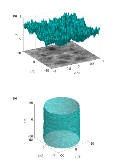
Figure 1: (a) An example of the 2D fractional Brownian motion function $f$, normalised to the range [0,1], shown as a surface plot and a heatmap. (b) The rough cylindrical boundary of our bucket is formed by using the surface in (a) to modulate the radius of the bucket boundary with an amplitude $a$. Here $a=0.1$.

To mimic the experimentally unavoidable surface roughness, we modify the azimuthal face of the bucket away from a perfect cylindrical shape using a noisy two-dimensional (2D) function. This function is numerically generated through a two-dimensional fractal Brownian motion MandelbrotVanNess with Hurst index of $0.3$, a parameter which describes the fractal dimension of the surface Mandelbrot1985 . The choice to model the roughness in this way is motivated by the well established fractal properties of real surfaces, including machined surfaces (of relevance to helium experiments), and the success of fractal brownian motion in modelling a wide variety of real rough surfaces Majumdar1990 . The function is normalised between $0$ and $1$, and is mirrored about its edge and recombined with itself in order to create periodicity across one dimension; a single realisation of the function is depicted in Fig. 1(a). The function is mapped onto the space of axial coordinate $z$ and azimuthal angle $\theta$, and used to modify the radius of the bucket according to the form,

$$r(z,\phi)=R(1-af(z,\theta)),$$ (5)

where $R$ is the smooth bucket radius and $a$ is the (dimensionless) roughness parameter. This numerical procedure generates all of our rough 3D bucket shapes. By computing the local curvature of the surface roughness, we find that the values of the average radius of curvature corresponding to values $a=0.05$, $0.1$, $0.2$ and $0.3$ of the roughness parameter are $10.4\xi$, $5.2\xi$, $2.6\xi$ and $1.7\xi$ respectively (small values of $a$ correspond to large radius of curvature, i.e. smoother surface). For simplicity, the top and bottom surfaces of the bucket are left smooth. The reason is that, by providing the vortex lines with pinning sites, any roughness on these surfaces will act essentially as an extra friction (an effect which already qualitatively account for via the dissipation parameter $\gamma$) slowing down the final stage of cristallization of the vortex lattice.

II.4 Simulation set-up

The initial condition for $\Psi$ in all of our simulations is the non-rotating ground state solution, found by the method of imaginary time propagation of the GPE, supplemented with low-amplitude white noise to $\Psi$ (amplitude $0.001$) to break any symmetries artificially presented in the initial condition. We then impose a constant rotation on the system for $t>0$, with fixed rotation frequency $\Omega$. Note that $\Omega$ far exceeds the critical rotation frequency to support vortices $\Omega_{\rm c}$, such that the lowest energy state of the fluid is a vortex lattice.

The non-dimensionalisation of the GPE is based on the natural units of the homogeneous fluid Barenghi2016 : the unit of length is the healing length $\xi$, the unit of speed is $c$, the unit of time is $\tau=\xi/c=\hbar/\mu_{0}$, the unit of energy is $\mu_{0}$, and the unit of density is $n_{0}$. Both our 3D and 2D numerical simulations are performed using XMDS2 xmds2 , an open-source partial and ordinary differential equation solver. The time evolution of the dimensionless GPE is computed via an adaptive fourth-fifth order Runge-Kutta integration scheme with typical time step $dt=0.01\tau$ and grid spacing $dx=0.4\xi$; these discretization numbers are sufficiently small to resolve the smallest spatial features (vortices and the fluid boundary layer, which are of the order of few healing lengths) and the shortest timescales in the fluid. We typically conduct our 3D simulations on a cubic grid of size $256^{3}$. Threaded parallel processing is employed using the OpenMP standard across typically $44$ threads to improve processing speeds on computationally intensive simulations.

III Results

III.1 Typical spin-up dynamics

(a)                                   (b)                                     (c)                                            

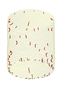
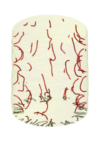
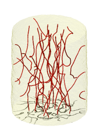
(d)                                     (e)                                   (f)                                  

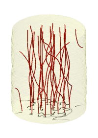
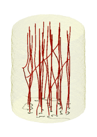
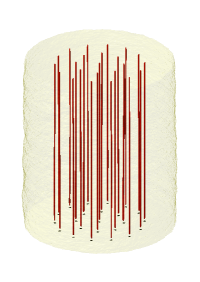
Figure 2: Three-dimensional snapshots at times $t/\tau=100$ (a), $200$ (b), $500$ (c), $1000$ (d), $1500$ (e) and $3000$ (f) during the spin-up of the initially quiescent fluid. The vortex cores are identified by density isosurfaces; vortices with positive and negative circulation (as determined by their pseudo-vorticity Villois2016 in the $z$ direction) are visualised in red and blue respectively. The faint yellow isosurface represents the confining bucket. A false-color shadow is projected onto the bottom surface to enhance the visualisation of the 3D vortex lines.

We now demonstrate the typical spin up of an initially quiescent fluid. Unless otherwise indicated, we present results for the following choice of parameters: bucket radius $R=50\xi$, bucket height $H=100\xi$, rotation frequency $\Omega=0.02~{}\tau^{-1}$, dissipation parameter $\gamma=0.05$, and roughness parameter $a=0.1$ (meaning that the irregular surface of the bucket extends radially from $45\rm\xi$ to $50~{}\xi$, corresponding to irregular ‘surface bumps’ of height up to 5 healing lengths).

The evolution of the fluid is illustrated by the snapshots shown in Fig. 2 in which the vortex lines are tracked in 3D space using a precise method introduced in Ref. Villois2016 ; movies of the evolution are available in Supplementary Material movies . From the initial quiescent and vortex-free fluid, first we see the nucleation of vortex lines at the cylindrical boundary of the fluid [Fig. 2(a)]. These vortices are all singly-quantized; we do not detect the presence of multiply-charged vortices in any of our simulations, which is consistent with the energetic instability of multiply-charged vortices and the favourability of singly-charged vortices Barenghi2016 . The nucleation takes place at the sharpest features on the surface, as seen in a previous calculation over a flat rough surface Stagg2017 : at these features the local (potential) flow velocity is raised by the curvature of the boundary, and exceeds the critical velocity of vortex nucleation, which, according to Landau’s criterion, in a Bose gas is $v_{c}\approx c$. Since the local flow speed around a moving obstacle always exceeds the translational speed of the obstacle, Landau’s criterion can be satisfied by a translational speed less than $c$. For example, a cylindrical obstacle moving at speed approximately equal to $0.4c$ will nucleate vortices Frisch1992 ; Stagg2014 . In our case ($\Omega=0.02/\tau$ and $R=50\xi$), the translational speed of the prominences on the rough boundary is approximately $\Omega R\approx c$, which is sufficient to exceed Landau’s criterion and nucleate vortices. Figure 2 (a) and (b) show that the vortex lines which nucleate at the rough boundary have the shape of small half-loops or handles; similar vortex shapes have been reported in trapped Bose-Einstein condensates Aftalion2003 and turbulent superfluid helium-4 near a heated cylinder Rickinson2020 , and have been called respectively “U-vortices” and “handles”.

We next consider the angular momentum of the fluid, exploring its evolution and distribution. We define the density of the $z$-component of the angular momentum of the fluid as,

$$L_{z}(x,y,z)=\psi^{*}i\hbar\left(y\frac{\partial}{\partial x}-x\frac{\partial}{\partial y}\right)\psi.$$ (6)

Figure 3(a) shows the angular momentum density as a function of the radial coordinate, averaged vertically and azimuthally, $\langle L_{z}\rangle$. At $t=0$, this is zero throughout the fluid. At time evolves, angular momentum builds at the edge of the bucket and drifts inwards, corresponding to the nucleation and inward drift of the vortex lines. At steady-state, the angular momentum forms a stepped curve, with each step corresponding to a concentric ring of vortex lines in the final lattice. Note how the final distribution of the angular momentum density approximately follows the result of solid-body rotation with constant mass density, $mn_{0}\Omega r^{2}$. The total $z$-component of the angular momentum $\mathcal{L}=\iiint L_{z}\,{\rm d}x\,{\rm d}y\,{\rm d}z$ (inset in Fig. 3(a)) grows in time, saturating at a final value by around $t\sim 2000~{}\tau$, which is when the vortex line have settled into the lattice configuration. In gaseous superfluids confined within smooth potentials, recent results of merging superfluids Kanai2018 ; Kanai2020 suggest that the rate of angular momentum transfer between a static and rotating state is constant; however, here the growth of the angular momentum follows a sigmoidal curve, rather than a linear one.

We also consider the distribution of the vortex length projected in the $z$-direction, $\Lambda_{z}$, as a function of radius, shown in Figure 3(b). At early times, vortex length exists only near the bucket edge, spreading progressively into the bulk. Later, the vortex length converges towards falling at discrete peaks at $r=0$, $r\approx 13\xi$ and $r\approx 26\xi$, corresponding to the concentric arrangement of vortices in the lattice configuration.

(a)

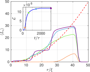
     (b)

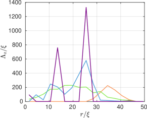
Figure 3: (a) Angular momentum density as a function of radius at various times during the spin-up of the rough bucket (same parameters as in Fig. 2). Plotted is the angular momentum density averaged over the $z$-dimension, $\langle L_{z}\rangle$. The lines correspond to times indicated by circular markers on the inset The distribution of the angular momentum of a solid-body of uniform density is shown by the red dashed line. The inset shows the evolution of the total angular momentum of the fluid $\mathcal{L}=\iiint L_{z}\,{\rm d}x\,{\rm d}y\,{\rm d}z$. (b) The vortex length projected in the $z$-direction $\Lambda_{z}$ plotted as a function of radius, at the same times as in (a). The data is binned in radial intervals of $3\xi$.

(a)

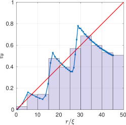
     (b)

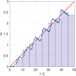
Figure 4: Azimuthal velocity $v_{\theta}$ of the fluid as a function of radius $r$, for rotation frequencies of $\Omega=0.02~{}\tau^{-1}$ (a) and $\Omega=0.06~{}\tau^{-1}$ (b). We use roughness parameter $a=0.1$. The solid red lines represent solid body rotation $v_{\theta}=\Omega r$; the blue lines are values of $v_{\theta}(r)$ averaged in the $\theta$ direction; the pale blue rectangles are histograms with bin size $\Delta r=5\xi$ (therefore the outer bins contain more data points). It is apparent that the more rapid rotation (b) creates a vortex lattice in better agreement with the solid body rotation, and that there is a vortex-free region near the boundary.

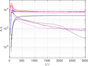
Figure 5: Evolution of the total vortex length, $\Lambda$ (solid lines), as well as the vortex length in the $z$-direction, $\Lambda_{z}$ (dashed lines) and the vortex length in the $xy$-plane, $\Lambda_{xy}$ (dot-dashed lines), plotted versus time $t$ for different angular velocity of rotation $\Omega=0.02~{}\tau^{{}_{1}}$ (black), $0.04~{}\tau^{-1}$ (blue) and $0.06~{}\tau^{-1}$ (red) achieving final values of the vortex length $\Lambda_{\infty}=2184\xi$, $6007\xi$ and $5568\xi$ respectively. All curves refer to roughness parameter $a=0.1$.

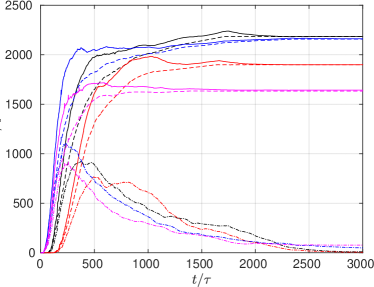
Figure 6: Evolution of the total vortex length, $\Lambda$ (solid lines), as well as the vortex length in the $z$-direction, $\Lambda_{z}$ (dashed lines) and the vortex length in the $xy$-plane, $\Lambda_{xy}$ (dot-dashed lines), plotted versus time $t$ for different boundary roughness $a=0.05$ (red), $0.1$ (black), $0.2$ (blue), and $0.3~{}\rm\xi$ (magenta), achieving final values $\Lambda_{\infty}=1899~{}\xi$, $2184~{}\xi$, $2161~{}\xi$ and $1643~{}\xi$. All curves refer to the same angular velocity $\Omega=0.02~{}\tau^{-1}$.

The collection of U-vortices nucleated at the boundary is the superfluid’s analog of a boundary layer, the region separating the rotating boundary from the still quiescent bulk of the fluid. The U-vortices tend to be aligned along the $z$-direction, creating a superflow in the same direction of the rotating boundary. The vortex nucleation is therefore short-lived, since the nucleated U-vortices reduce the relative motion between the fluid and the boundary, suppressing further nucleations. In time, the U-vortices grow in size and extend further into the fluid [Fig. 2(b,c)], ultimately filling the bulk [Fig. 2(d)]. During this stage of the evolution, the U-vortices also grow in vertical extent in the $z$-direction, occasionally connecting and merging with each other, thus increasing their vertical extent. When the length in the $z$-direction becomes of the order of the bucket’s height $H$, one or both vortex endpoints start sliding along the smooth top and/or bottom of the bucket. Once most of the vortex lines are fully extended from the top to the bottom of the bucket, they quickly drift into the bulk of the fluid. Although the vortex lines are aligned along the direction of rotation, they remain highly excited and undergo reconnection events when they collide with each other. Over time they relax towards a regular configuration of straight vortices. A small proportion of U-vortices remain attached to the side of the bucket for a longer period of time [Fig. 2(d)]; over a longer time they detach, and relax to the final lattice configuration. Some of the vortex lines end up diagonally across the rest of the vortex lattice [Fig. 2(e)]: eventually they also relax to the final lattice configuration [Fig. 2(f)]. The vortex lattice is stationary in the rotating frame, representing the lowest energy state of the rotating superfluid. In this final state, the coarse-grained fluid velocity approximates the solid-body result ${\bf v}=v_{\theta}\,{\bf e_{\theta}}=\Omega\,r\,{\bf e_{\theta}}$, where ${\bf e_{\phi}}$ is the azimuthal unit vector, as shown in Fig. 4; as expected, the agreement improves with increasing $\Omega$, and there is a vortex-free region near the boundary.

Our 3D results are presented for a fixed bucket size due to computational constraints of simulating a larger system. For a larger bucket we would expect qualitatively similar dynamics; indeed our 2D results in a larger bucket presented in Section IV C support this. The most significant change under a larger bucket is more vortices in the final state (at a fixed rotation frequency) and as a result a better approximation to solid-body rotation.

III.2 Role of angular velocity and roughness

To analyse the vortex dynamics further it is useful to distinguish the total vortex length, $\Lambda$, from the vortex length projected in the $z$-direction, $\Lambda_{z}$, and the vortex length projected in the $xy$-plane, $\Lambda_{xy}$. In the final vortex lattice all vortex lines are aligned along $z$, hence we expect that, after a sufficiently long time, $\Lambda_{xy}\approx 0$ and $\Lambda_{z}\approx\Lambda$, with $\Lambda\rightarrow N_{v}H$, where $N_{v}$ is the final number of straight vortex lines. Figure 5 displays $\Lambda$ (solid lines), $\Lambda_{z}$ (dashed lines) and $\Lambda_{xy}$ (dot-dashed lines) as a function of time for different angular velocities of rotation, $\Omega=0.02$, $0.04$ and $0.06$ at the same roughness parameter $a=0.1$. It is apparent that in the initial stage, a great amount of vorticity is in the $xy$-plane, before realignment of the vortex lines along the $z$-axis of rotation takes place. The effect is particularly noticeable at the largest angular velocities, for which, during the initial transient, the vortex length is considerably larger than the value $\Lambda_{\infty}$ achieved in the final vortex lattice configuration. Moreover, we see that the final vortex line length increases with $\Omega$ due to the increasing number of vortices in the final state.

Figure 6 shows $\Lambda$, $\Lambda_{z}$ and $\Lambda_{xy}$ plotted versus time at the same angular velocity $\Omega=0.02~{}\tau^{-1}$ for different values of roughness parameter $a$. The largest values of the final vortex length $\Lambda_{\infty}$ are achieved with $a=0.1\xi$ and $a=0.2\xi$. Smoother ($a=0.05\xi$) and rougher ($a=0.3\xi$) boundaries generate less vortex length. These variations in the final line length arise to the final number of vortex lines varying by a few vortices across these cases. It is not surprising that the final vortex lattice depends on the roughness which has nucleated the initial vorticity. Feynman’s rule [Eq. (2)] only refers to an idealised homogeneous system. Boundaries are known to have effects (e.g. missing vortex lines near the boundary) and it has been observed that the formation of the vortex lattice may be history-dependent and involve metastability CampbellZiff ; Wood2019 and hysteresis Mathieu .

Figure 7 compares the growth of angular momentum between the default case (blue line), the case where the rotation frequency is doubled (red line), and the case where the roughness amplitude is doubled (yellow line). The growth behaviour is qualitatively similar in all cases. Doubling the rotation frequency leads to a much faster rate of injection of angular momentum, and a higher final value, consistent with the faster injection rate of vortex lines from the boundary and the higher density of vortex lines in the final lattice state. Doubling the surface roughness has little effect on the growth of the angular momentum, just slightly increasing the rate of angular momentum injection, which can be attributed to the greater injection rate of vortices from the rougher surface.

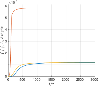
Figure 7: Evolution of the total angular momentum for the default parameters used in Fig. 2 (blue line), double the rotation frequency (red line) and double the roughness amplitude (yellow line).

(a)                                   (b)                                     (c)                                                             

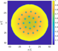
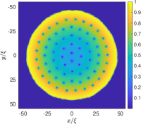
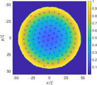
(d)                                     (e)                                   (f)                                  

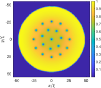
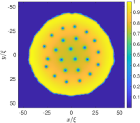
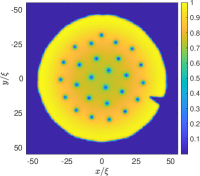
Figure 8: Density profile in the $xy$-plane at the half-height of the bucket, showing the final vortex configurations for the following cases: (a): $\Omega=0.02~{}\tau^{-1}$ and $a=0.1$ (default choice); (b): $\Omega=0.04~{}\tau^{-1}$ and $a=0.1$ (double rotation); (c): $\Omega=0.06~{}\tau^{-1}$ and $a=0.1$ (triple rotation); (d): $\Omega=0.02~{}\tau^{-1}$ and $a=0.05$ (half roughness); (e): $\Omega=0.02~{}\tau^{-1}$ and $a=0.2$ (double roughness); (f): $\Omega=0.02~{}\tau^{-1}$ and $a=0.1$ (single strong protuberance added, see Section IV).

Figure 8 illustrates some of the final vortex patterns which we have computed by plotting the superfluid density, $|\psi(x,y)|^{2}$ in the $xy$-plane at half-height of the bucket. In these pictures the vortices appear as small holes; to clarify the lengthscales, we recall that on the vortex axis the density is zero and that at distance $r=2\xi$ from the axis, the density recovers about $80\%$ of the bulk value at infinity. It is interesting to compare the different final vortex configurations for halved/doubled rotation velocity and the roughness parameter with respect to our default choice ($\Omega=0.02~{}\tau^{-1}$ and $a=0.1$). While the ideal 2D vortex lattice has a vortex at the centre, surrounded by a first row of 6 vortices, a second row of 12 vortices, etc, the vortex configurations shown in Fig. 8 contain slightly different vortex numbers; in particular some configurations contain vortex lines which seem misplaced [Fig. 8(c)] or lack the vortex at the centre [Fig. 8(e)]; these configurations are metastable states corresponding to local minima of the free energy in the rotating frame CampbellZiff . Moreover, at slow rotations [Fig. 8(a,d)] the predicted vortex-free region near the boundary NorthbyDonnelly1970 ; ShenkMehl1971 ; StaufferFetter1968 is clearly visible; this phenomenon affects the coarse-grained azimuthal velocity near the boundary shown previously in Fig. 4(a). The depletion of the background fluid density in the centre of the bucket - particularly evident in Fig. 8(b) and (c) - is due to coarse-grained centrifugal effects, analogous to the classical rotating case Barenghi2016 .

IV Other effects

In this section we repeat the simulation of Section III with several significantly modifications: the presence of a single strong protuberance, the presence of remanent vortex lines, and the 2D case. The aim is to determine whether these effects change qualitatively the dynamics described in Section III.

IV.1 Effect of a strong protubance

(a)                           (b)                          (c)                           (d)                           (e)          

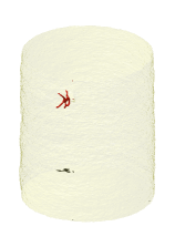
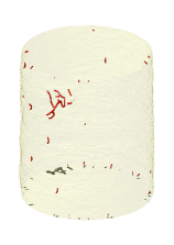
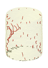
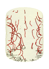
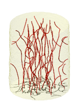
Figure 9: Early-time dynamics during the spin-up of the fluid in the presence of a single strong protuberance added to the rough cylindrical boundary. The snapshots, taken at $t/\tau=26$, $50$, $100$, $200$ and $500$, are presented in the same way as Fig. 2.

First we consider the effect of a single strong imperfection in the form of a protuberance on the cylindrical wall. The question is whether, by enhancing vortex nucleation, the protuberance can induce a turbulent boundary layer. The protuberance is numerically created by adding a Gaussian-shaped potential to the existing (small-scale) roughness potential. Equation (5) is replaced by

$$r(z,\phi)=R[1-a(f(z,\theta)+Gf_{G}(z,\theta))],$$ (7)

where $G=2$ and $f_{G}(z,\theta)$ is a Gaussian-shape function taking values from $0$ to $1$ and rms width $4\xi$. The approximate height of the strong protuberance in the simulation which we present is $10\xi$, as also visible in Fig. 8(f).

Snapshots taken during the time evolution for $\Omega=0.02~{}\tau^{-1}$ and $a=0.1$ are shown in Fig. 9; a movie can be viewed in Supplementary Material movie_gaussian . The protuberance catalyses the local nucleation of vortices at early times: large vortex loops (of the same size order as the protuberance) are rapidly generated [Fig. 9(a)], leading to a downstream trail of loops [Fig. 9(b, c)], in addition to the slower nucleation of U-vortices from the rough bucket wall. The vortex configuration becomes clearly anisotropic near the bucket edge [Fig. 9(d)]. However, once the vortices fill the bulk [Fig. 9(e)], memory of this effect is lost, and the subsequent evolution is very similar to the evolution without the strong protuberance. In fact, the final vortex lattice is not significantly different from the lattices considered in Section III, as shown in Fig. 8(f). Figure 10 shows the time evolution of $\Lambda$, $\Lambda_{z}$ and $\Lambda_{xy}$ in the presence of the protuberance (magenta lines) and its absence (black lines). This confirms that the protuberance accelerates the generation of vortex line length at early times, but that its effect becomes washed out at later times.

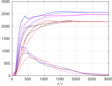
Figure 10: Time evolution of $\Lambda$ (solid line), $\Lambda_{z}$ (dashed line), $\Lambda_{xy}$ (dot-dashed line). The colours correspond to the simulations with default parameters $\Omega=0.02\tau^{-1}$, $a=0.1\xi$ (black), the added surface protuberance (magenta), the added remanent negative vortex (blue), and the added remanent positive vortex (red), respectively.

IV.2 Effect of remanent vortices

Secondly, we consider the effect of remanent vortex lines. In experiments with liquid helium, it is believed that so-called ‘remanent vortices’ may be present in the fluid, created via the Kibble-Zurek mechanism when cooling the helium sample through the superfluid transition to the final experimental temperature. The presence of remanent vortices may modify the vortex nucleation and the formation of the vortex lattice when the sample is rotated. To explore this idea, we have repeated the simulations imposing a suitable phase profile to add a vortex to the initial state during the imaginary-time propagation. For simplicity we position the remanent vortex along the $z$-axis of rotation.

The evolution of the superfluid with the standard rough cylindrical wall and a “positive” remanent vortex, that is, one whose circulation is oriented in the same direction of the bucket’s rotation is shown through Fig. 11 and the movie in the Supplementary Material movie_pos_remnant . Compared to Section III, the only significant modification is a dampening of the initial injection of U-vortices; the effect is visible by eye when comparing like-time snapshots [Fig. 2(b) and Fig. 11(a)]. The remanent vortex acts in the same direction as the rotating container: it reduces the relative speed between the bucket’s wall and the superfluid, and remains largely undisturbed at early times [Fig. 11(a)] until the U-vortices that are nucleated fill the bulk and interact with it [Fig. 11(b)]; at this point the remanent vortex becomes subsumed within the other like-signed vortices [Fig. 11(c)], and the subsequent relaxation of the vortex configuration into a vortex lattice largely proceeds as if there was not any remanent vortex initially. Confirming this, we see that in Figure 10 that the presence of the positive vortex (red lines) depletes the generation of vortex line length at early times, but this recovers at later times such that the system reaches the same line length as in the absence of any remanent vortices (black lines).

(a)                                  (b)                                    (c)

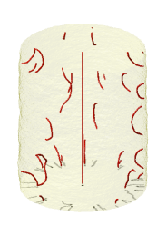
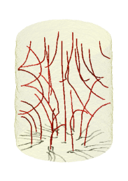
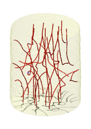
Figure 11: Spin-up of the superfluid in the presence of a positively-charged remanent vortex. Snapshots are taken at $t/\tau=200$, $400$ and $500$, and are presented in the same way as Fig. 2.

(a)                                  (b)                              (c)    (d)                                  (e)                             

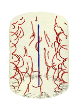
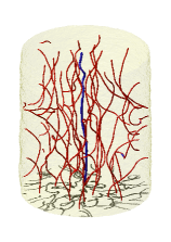
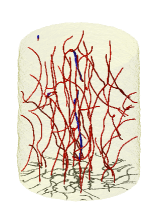
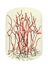
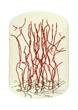
Figure 12: Spin-up of the superfluid in the presence of a negatively-charged remanent vortex. Snapshots are taken at $t/\tau=200$ (a), $360$ (b), $386$ (c), $420$ (d) and $500$ (e). The images are presented in the same way as Fig. 2. Vortices with negative circulation are coloured blue.

If the remanent vortex is oriented in the direction opposite to the rotation of the bucket, i.e. a negative vortex, the evolution proceeds differently, as seen in Fig. 12 and the movie in Supplementary Material movie_neg_remnant . The remanent vortex enhances the nucleation of U-vortices from the boundary, as evident from comparing Fig. 2(b) and Fig. 12(a). This effect is caused by the counter-flow induced by the remanent vortex, which increases the relative speed of the fluid over the rough boundary. Once the other vortices drift close to the remanent vortex, the remanent vortex becomes excited by their interaction [Fig. 12(b)]. A series of vortex reconnections break up the remanent vortex, forming progressively smaller vortex loops [Fig. 12(c,d)]. This leads to the rapid removal of vorticity of the ‘wrong’ sign from the fluid [Fig. 12(e)]. Hereafter the fluid evolves in a similar manner to when the remanent vortex in absent [Section III], albeit with a slightly higher final vortex line length [Fig. 10].

IV.3 2D case

Finally, we have also performed the corresponding 2D simulations of the spin-up of a 2D superfluid within a rough circular boundary; the boundary is taken from the central slice of the 3D rough bucket. A movie showing the typical dynamics is available in the Supplementary Material movie_2d_large_bucket . The 2D geometry allows calculations of much larger buckets, up to $R=200\xi$ with a $1024^{2}$ numerical grid. We observe the same qualitative behaviour as in 3D in smaller buckets, albeit with many more vortices and without 3D effects such as vortex reconnections. Collisions of vortices of the opposite circulation result in the annihilation of the vortices and the emission of sound pulses Kwon2014 ; Stagg2015 ; Groszek2016 . In general, we find that, in 2D, the timescales of injection, diffusion and lattice crystallisation are faster than in 3D. A particular feature that we see in the early-time dynamics of the 2D simulations is the nucleation of vortices with both positive and negative circulation (i.e. with circulation which is inconsistent with the imposed rotation). We notice that some negative vortices originate from localised rarefaction pulses generated from the rough boundary when the bucket is set into rotation. We associate these pulses with Jones-Roberts solitons Jones1982 ; Tsuchiya2008 , which are low energy/momentum solutions of the 2D GPE. At higher energy/momentum, these solutions become pairs of vortices of opposite sign (also called vortex dipoles in the literature). The conversion of Jones-Roberts solitons into vortex dipoles occurs if the pulse gains energy from the large positive vortex cluster which starts forming in the centre of the bucket. Occasionally, the vortices which are parts of a dipole separate and mix with the rest of the vortices. Over time, the vortices of negative circulation are lost from the system, either colliding (hence annihilating) with positive vortices within the bulk, or by exiting the fluid at the bucket’s boundary (effectively annihilating with their images).

V Conclusions

In conclusion, we have employed simulations of the Gross-Pitaevskii equation to study the spin-up of a superfluid in a rotating bucket featuring microscopically rough walls. Within this model, we see several key stages of the dynamics. Firstly, vortices are nucleated at the boundary by the flow over the rough features, typically in the form of small U-shaped vortex lines. Secondly, these U-shaped vortices interact strongly and reconnect, creating a transient turbulent state. This becomes increasingly polarised by the imposed rotation until the vortex configuration consists of vortices of the correct orientation extending from the top to the bottom of the bucket. Finally, the vortex lines slowly straighten and arrange themselves in the expected final vortex lattice configuration. Our results highlight the importance of vortex reconnections Galantucci2019 : it is generally assumed that vortex reconnections are important in turbulence, but here we have seen that reconnections are essential to create, starting from potential flow, something as simple as solid body rotation (the vortex lattice). The addition of a single large protuberance or one additional remanent vortex line does not change the dynamics significantly, only speeding up or slowing down the injection of vorticity. Moreover, analogous dynamics arise in the 2D limit.

We reiterate that the GPE is not a quantitatvely accurate model of superfluid helium and these results should be interpreted qualitatively only. For example, the role of friction is introduced into the GPE through a widely-used phenomenological dissipation term; however, a more accurate physical model of this stage of the dynamics would be provided by the VFM. Also, a distinctive physical property of superfluid helium is its strong non-local interactions. This, for instance, supports a roton minimum in its excitation spectrum. While this is absent from the GPE model we have employed, it can be introduced through an additional non-local term Berloff2014 ; Reneuve2018 . It would be interesting to see if this causes any significant departures from the dynamics we have reported.

References

- (1) J. F. Annett, Superconductivity, Superfluids and Condensates (Oxford University Press, Oxford, 2004).
- (2) C. F. Barenghi and N. G. Parker, A Primer on Quantum Fluids (Springer, Berlin, 2016).
- (3) E. J. Yarmchuck, M. J. V. Gordon, R. E. Packard, Phys. Rev. Lett. 43, 214 (1979).
- (4) G.P. Bewley, D.P. Lathrop and K.R. Sreenivasan, Nature 441, 588 (2006)
- (5) K. W. Madison, F. Chevy, W. Wohlleben and J. Dalibard, J. Mod. Opt. 47, 2715 (2000)
- (6) J. R. Abo-Shaeer, C.Raman, J. M. Vogels and W. Ketterle, Science 292, 476 (2001).
- (7) D. S. Tsakadze, Sov. Phys. JETP 19, 110 (1964).
- (8) C. Josserand, Chaos 14, 875 (2004).
- (9) K. Kasamatsu, M. Tsubota, and M. Ueda, Phys. Rev. A 66, 053606 (2002).
- (10) U. R. Fischer, and G. Baym, Phys. Rev. Lett. 90, 140402 (2003).
- (11) G. M. Kavoulakis, and G. Baym, New J. Phys. 5, 51 (2003).
- (12) P. Engels, I. Coddington, P. C. Haljan, V. Schweikhard, and E. A. Cornell, Phys. Rev. Lett. 90, 170405 (2003).
- (13) K. W. Schwarz, Phys. Rev. Lett. 64, 1130 (1990).
- (14) N. Hashimoto, R. Goto, H. Yano, K. Obara, O. Ishikawa and T. Hata, Phys. Rev. B 76, 020504(R) (2007).
- (15) D. E. Zmeev, F. Pakpour, P. M. Walmsley, A. I. Golov, W. Guo, D. N. McKinsey, G. G. Ihas, P. V. E. McClintock, S. N. Fisher and W. F. Vinen, Phys. Rev. Lett. 110, 175303 (2013).
- (16) D. Duda, P. S̆vanc̆ara, M. La Mantia, M. Rotter and L. Skrbek, Phys. Rev. B 92, 064519 (2015).
- (17) A. L. Fetter, Phys. Rev. 152, 183 (1966)
- (18) D. Stauffer and A. L. Fetter, Phys. Rev. 168, 156 (1968).
- (19) G. W. Stagg, N. G. Parker and C. F. Barenghi, Phys. Rev. Lett. 118, 135301 (2017).
- (20) C. M. Muirhead, W. F. Vinen, and R. J. Donnelly, Phil. Trans. R. Soc. Lond. A 311, 433 (1984).
- (21) P. V. E. McClintock and R. M. Bowley, in Progress in Low Temperature Physics, vol. 14. pages 1-68 (1995).
- (22) N. G. Berloff and P. H. Roberts, Phys. Lett. A 274, 69 (2000).
- (23) T. Winiecki and C. S. Adams, Europhys. Lett. 52, 257 (2000).
- (24) A. Villois and H. Salman, Phys. Rev. B 97, 094507 (2018).
- (25) K. W. Schwarz, Phys. Rev. B 38, 2398 (1988).
- (26) K. W. Schwarz, Phys. Rev. B 31, 5782 (1985).
- (27) M. Tsubota and S. Maekawa, Phys. Rev. B 47, 12040 (1993)
- (28) K. W. Schwarz, Phys. Rev. A 10, 2306 (1974).
- (29) D. Kivotides, C. F. Barenghi, and Y. A. Sergeev, J. Low Temp. Phys. 144, 121 (2006).
- (30) R. Hänninen and A. W. Baggaley, Proc. Nat. Acad. Sci USA 111 (suppl. 1), 4667 (2014).
- (31) R. Hänninen, A. Mitani, and M. Tsubota, J. Low Temp. Phys. 138, 589 (2005).
- (32) L. Pitaevskii and S. Stringari, Bose-Einstein Condensation (Oxford University Press, Oxford, 2003)
- (33) S. Choi, S. A. Morgan, and K. Burnett, Phys. Rev. A 57, 4057 (1998).
- (34) M. Tsubota, K. Kasamatsu, and M. Ueda, Phys. Rev. A 65 023603 (2001).
- (35) B. B. Mandelbrot and J. W. Van Ness, SIAM Rev., 10, 422 (1968),
- (36) B. B. Mandelbrot, Physica Scripta 32, 257 (1985).
- (37) A. Majumdar and B. Bhushan, J. Tribol. 112, 205 (1990).
- (38) G. R. Dennis, J. J. Hope, and M. T. Johnsson, Comput. Phys. Commun. 184, 201-208 (2013)
- (39) A. Villois, G. Krstulovic, D. Proment and H. Salman, J. Phys. A: Math. Theor. 49, 415502 (2016)
-
(40)
movie_ref(3D view) andmovie_2d_midslicein Supplementary Material. - (41) T. Frisch, Y. Pomeau and S. Rica, Phys. Rev. Lett. 69, 1644 (1992)
- (42) G. W. Stagg, N. G. Parker and C. F. Barenghi, J. Phys. B: At. Mol. Opt. Phys. 47, 095304 (2014)
- (43) A. Aftalion and I. Danaila, Phys. Rev. A 68, 023603 (2003).
- (44) E. Rickinson, C. F. Barenghi, Y. A. Sergeev, A. W. Baggaley, Phys. Rev. B 101, 134519 (2020).
- (45) T. Kanai, W. Guo and M. Tsubota, Phys. Rev. A 97, 013612 (2018).
- (46) T. Kanai, W. Guo, M. Tsubota and D. Jin, Phys. Rev. Lett., 124, 105302 (2020)
- (47) L. J. Campbell and R. M. Ziff, Phys. Rev. B 2, 1886 (1979).
- (48) T. S. Wood, M. Mesgarnezhad, G. W. Stagg, and C. F. Barenghi, Phys. Rev. B 100, 024505 (2019).
- (49) P. Mathieu, J. C. Marechal, and Y. Simon, Phys. Rev. B 22, 4293 (1980).
- (50) J.A. Northby and R. J. Donnelly, Phys. Rev. Lett. 25, 214 (1970.
- (51) D. S. Shenk and J. B. Mehl Phys. Rev. Lett. 27, 1703 (1971).
-
(52)
movie_gaussianin Supplementary Material. -
(53)
movie_pos_remnantin Supplementary Material. -
(54)
movie_neg_remnantin Supplementary Material. -
(55)
movie_2d_large_bucketin Supplementary Material. - (56) W. J. Kwon, G. Moon, J-y. Choi, S. W. Seo and Y-i. Shin, Phys. Rev. A 90, 063627 (2014)
- (57) G. W. Stagg, A. J. Allen, N. G. Parker and C. F. Barenghi, Phys. Rev. A 91, 013612 (2015)
- (58) A. J. Groszek, T. P. Simula, D. M. Paganin and K. Helmerson, Phys. Rev. A 93, 043614 (2016)
- (59) C. A. Jones and P. H. Roberts, J. Phys. A: Math. Gen. 15, 2599 (1982)
- (60) S. Tsuchiya, F. Dalfovo and L. Pitaevskii, Phys. Rev. A 77, 045601 (2008).
- (61) L. Galantucci, A.W. Baggaley, N.G. Parker, and C.F. Barenghi, Proc. Nat. Acad. Sci. USA 116, 12204 (2019).
- (62) N. Berloff, M. Brachet and N. P. Proukakis, Proc. Natl. Acad. Sci. USA 111, 4675 (2014).
- (63) J. Reneuve, J. Salort and L. Chevillard, Phys. Rev. Fluids 3, 114602 (2018).