Dynamics of Colombo’s Top: Generating Exoplanet Obliquities from Planet-Disk Interactions

Abstract

Large planetary spin-orbit misalignments (obliquities) may strongly influence atmospheric circulation and tidal heating in the planet. A promising avenue to generate obliquities is via spin-orbit resonances, where the spin and orbital precession frequencies of the planet cross each other as the system evolves in time. One such mechanism involves a dissipating (mass-losing) protoplanetary disk that drives orbital precession of an interior planet. We study this scenario analytically in this paper, and obtain the mapping between the general initial spin orientation and the final obliquity. We show that (i) under adiabatic evolution (i.e. the disk dissipates at a sufficiently slow rate), the final planetary obliquity as a function of the initial spin orientation bifurcates into distinct tracks governed by interactions with the resonance; (ii) under nonadiabatic evolution, a broad range of obliquities can be excited. We obtain analytical expressions for the final obliquities for various regimes of parameter space. The dynamical system studied in this paper is an example of “Colombo’s top”, and our analysis and results can be adapted to other applications.

1 Introduction

1.1 Colombo’s Top

A rotating planet is subjected to gravitational torque from its host star, making its spin axis precess around its orbital (angular momentum) axis. Now suppose the orbital axis precesses around another fixed axis—such orbital precession could arise from gravitational interactions with other masses in the system (e.g. planets, external disks, or binary stellar companion). What is the dynamics of the planetary spin axis? How does the spin axis evolve as the spin precession rate, the orbital precession rate, or their ratio, gradually changes in time?

Colombo (1966) was the first to point out the importance of the above simple model in the study of the obliquity (the angle between the spin and orbital axes) of planets and satellites. Subsequent works (Peale, 1969, 1974; Ward, 1975; Henrard & Murigande, 1987) have revealed rich dynamics of this model. With appropriate modification, this model can be used as a basis for understanding the evolution of rotation axes of celestial bodies. Indeed, many contemporary problems in planetary/exoplanetary dynamics can be cast into a form analogous to this simple model or its variants (e.g. Ward & Hamilton, 2004; Fabrycky et al., 2007; Batygin & Adams, 2013; Lai, 2014; Anderson & Lai, 2018; Zanazzi & Lai, 2018).

In this paper we present a systematic investigation on the secular evolution of Colombo’s top, starting from general initial conditions. Our study includes several new analytical results that go beyond previous works. While our results are general, we frame our study in the context of generating exoplanet obliquities from planet-disk interaction with a dissipating disk.

1.2 Planetary Obliquities from Planet-Disk Interaction

It is well recognized that the obliquity of a planet may provide important clues to its dynamical history. In the the Solar System, a wide range of planetary obliquities are observed, from nearly zero for Mercury and $3.1^{\circ}$ for Jupiter, to $23^{\circ}$ for Earth and $26.7^{\circ}$ for Saturn, to $98^{\circ}$ for Uranus. Multiple giant impacts are traditionally invoked to generate the large obliquities of ice giants (Safronov & Zvjagina, 1969; Benz et al., 1989; Korycansky et al., 1990; Morbidelli et al., 2012). For gas giants, obliquity excitation may be achieved via spin-orbit resonances, where the spin and orbital precession frequencies of the planet become commensurate as the system evolves (Ward & Hamilton, 2004; Hamilton & Ward, 2004; Vokrouhlickỳ & Nesvornỳ, 2015). Such resonances may also play a role in generating the obliquities of Uranus and Neptune (Rogoszinski & Hamilton, 2019). For terrestrial planets, multiple spin-orbit resonances and their overlaps can make the obliquity vary chaotically over a wide range (e.g. Laskar & Robutel, 1993; Touma & Wisdom, 1993; Correia et al., 2003)

Obliquities of extrasolar planets are difficult to measure. So far only loose constraints have been obtained for the obliquity of a faraway ($\gtrsim 50$ au) planetary-mass companion (Bryan et al., 2020). But there are prospects for constraining exoplanetary obliquities in the coming years, such as using high-resolution spectroscopy to obtain $v\sin i$ of the planet (Snellen et al., 2014; Bryan et al., 2018) and using high-precision photometry to measure asphericity of the planet (Seager & Hui, 2002). Finite planetary obliquities have been indirectly inferred to explain the peculiar thermal phase curves (see e.g. Adams et al., 2019; Ohno & Zhang, 2019) and tidal dissipation in hot Jupiters (Millholland & Laughlin, 2018) and in super-Earths (Millholland & Laughlin, 2019).

It is natural to imagine some of the mechanisms that generate planetary obliquities in the Solar System may also operate in exoplanetary systems. Recently, Millholland & Batygin (2019) studied the production of planet obliquities via a spin-orbit resonance, where a dissipating protoplanetary disk causes resonance capture and advection. In their work, a planet is accompanied by an inclined exterior disk; as the disk gradually dissipates, the planetary obliquity increases, reaching $90^{\circ}$ for what the authors characterize as adiabatic resonance crossings.

The Millholland & Batygin study assumes a negligible initial planetary obliquity. This assumption is intuitive, since the planet attains its spin angular momentum from the disk. But it may not always be satisfied. In particular, the formation of rocky planets through planetesimal accretion can lead to a wide range of obliquities, especially if the final spin is imparted by a few large bodies (Dones & Tremaine, 1993; Lissauer et al., 1997; Miguel & Brunini, 2010). Such “stochastic” accretion likely happened for terrestrial planets in the Solar System. Giant impacts may have also played a role in the formation of the close-in multiple-planet systems diskovered by the Kepler satellite (e.g. Inamdar & Schlichting, 2015; Izidoro et al., 2017).

1.3 Goal of This Paper

In this paper, we consider a wide range of initial planetary obliquities in the Millholland-Batygin dissipating disk scenario, and examine how the obliquity evolves toward the “final” value as the exterior disk dissipates. We provide an analytical framework for understanding the final planetary obliquity for arbitrary initial spin-disk misalignment angles. We also consider various dissipation timescales, and examine both “adiabatic” (slow disk dissipation) and “non-adiabatic” evolution. We calibrate these analytical results with numerical calculations. On the technical side, our paper extends previous works (such as Henrard, 1982; Henrard & Murigande, 1987; Millholland & Batygin, 2019) in several aspects. Two of our main results are: (i) a careful accounting of the phase space area across sepratrix to analytically describe the rich dynamics of adiabatic evolution, and (ii) using the concept of “partial adiabatic resonance advection” to fully capture the dynamics in the non-adiabatic limit.

It is important to note that while we focus on a specific scenario of generating/modifying planetary obliquities from planet-disk interactions, our analysis and results have a wide range of applicability. For example, a dissipating disk is dynamically equivalent to an outward-migrating external companion.

The paper is organized as follows. In Section 2, we review the relevant spin-orbit dynamics and key concepts that are used in the remainder of the paper. In Sections 3 and 4, we study the evolution of the system when the disk dissipates on different timescales, from highly adiabatic to nonadiabatic. Analytical results are presented to explain the numerical results in both limits. We discuss the implications of our results in Section 5. Our primary physical results consist of Fig. 5 in the adiabatic limit and Fig. 12 in the nonadiabatic limit. Some detailed calculations are relegated to the appendices, including a leading-order estimate of the final planetary obliquities given small initial spin-disk misalignment angles in Appendix B.

2 Theory

2.1 Equations of Motion

We consider a star of mass $M_{\star}$ hosting an oblate planet (mass $M_{\rm p}$, radius $R_{\rm p}$ and spin angular frequency $\Omega_{\rm p}$) at semimajor axis $a_{\rm p}$, and a protoplanetary disk of mass $M_{\rm d}$. For simplicity, we treat the disk as a ring of radius $r_{\rm d}$, but it is simple to generalize to a disk with finite extent (see Millholland & Batygin, 2019). Denote $\boldsymbol{\mathbf{S}}$ the spin angular momentum and $\boldsymbol{\mathbf{L}}$ the orbital angular momentum of the planet, and $\boldsymbol{\mathbf{L}}_{\rm d}$ the angular momentum of the disk. The corresponding unit vectors are $\hat{\boldsymbol{\mathbf{s}}}\equiv\boldsymbol{\mathbf{S}}/S$, $\hat{\boldsymbol{\mathbf{l}}}\equiv\boldsymbol{\mathbf{L}}/L$, and $\hat{\boldsymbol{\mathbf{l}}}_{\rm d}\equiv\boldsymbol{\mathbf{L}}_{\rm d}/L_{\rm d}$.

The spin axis $\hat{\boldsymbol{\mathbf{s}}}$ of the planet tends to precess around its orbital (angular momentum) axis $\hat{\boldsymbol{\mathbf{l}}}$, driven by the gravitational torque from the host star acting on the planet’s rotational bulge. On the other hand, $\hat{\boldsymbol{\mathbf{l}}}$ and the disk axis $\hat{\boldsymbol{\mathbf{l}}}_{\rm d}$ precess around each other due to gravitational interactions. We assume $S\ll L\ll L_{\rm d}$, so $\hat{\boldsymbol{\mathbf{l}}}_{\rm d}$ is nearly constant and $\hat{\boldsymbol{\mathbf{l}}}$ experiences negligible backreaction torque from $\hat{\boldsymbol{\mathbf{s}}}$. The equations of motion for $\hat{\boldsymbol{\mathbf{s}}}$ and $\hat{\boldsymbol{\mathbf{l}}}$ in this limit are (Anderson & Lai, 2018)

$$\frac{\mathrm{d}\hat{\boldsymbol{\mathbf{s}}}}{\mathrm{d}t} =\omega_{\rm sl}\left(\hat{\boldsymbol{\mathbf{s}}}\cdot\hat{\boldsymbol{\mathbf{l}}}\right)\left(\hat{\boldsymbol{\mathbf{s}}}\times\hat{\boldsymbol{\mathbf{l}}}\right)\equiv\alpha\left(\hat{\boldsymbol{\mathbf{s}}}\cdot\hat{\boldsymbol{\mathbf{l}}}\right)\left(\hat{\boldsymbol{\mathbf{s}}}\times\hat{\boldsymbol{\mathbf{l}}}\right),$$ (1)

$$\frac{\mathrm{d}\hat{\boldsymbol{\mathbf{l}}}}{\mathrm{d}t} =\omega_{\rm ld}\left(\hat{\boldsymbol{\mathbf{l}}}\cdot\hat{\boldsymbol{\mathbf{l}}}_{\rm d}\right)\left(\hat{\boldsymbol{\mathbf{l}}}\times\hat{\boldsymbol{\mathbf{l}}}_{\rm d}\right)\equiv-g\left(\hat{\boldsymbol{\mathbf{l}}}\times\hat{\boldsymbol{\mathbf{l}}}_{\rm d}\right),$$ (2)

where

$$\omega_{\rm sl} \equiv\frac{3GJ_{2}M_{p}R_{p}^{2}M_{\star}}{2a_{p}^{3}I_{p}\Omega_{p}}=\frac{3k_{\rm qp}}{2k_{\rm p}}\frac{M_{\star}}{m_{\rm p}}\left(\frac{R_{\rm p}}{a_{\rm p}}\right)^{3}\Omega_{\rm p},$$ (3)

$$\omega_{\rm ld} \equiv\frac{3M_{\rm d}}{4M_{\star}}\left(\frac{a_{\rm p}}{r_{\rm d}}\right)^{3}n.$$ (4)

In Eq. (3), $I_{p}=k_{p}M_{p}R_{p}^{2}$ (with $k_{p}$ a constant) is the moment of inertia and $J_{2}=k_{\rm qp}\Omega_{p}^{2}(R_{p}^{3}/GM_{p})$ (with $k_{qp}$ a constant) the rotation-induced (dimensionless) quadrupole of the planet [for a body with uniform density, $k_{p}=0.4,k_{qp}=0.5$; for giant planets, $k_{p}\simeq 0.25$ and $k_{qp}\simeq 0.17$ (e.g. Lainey, 2016)]. In other studies, $3k_{\rm qp}/2k_{\rm p}$ is often notated as $k_{2}/2C$ (e.g. Millholland & Batygin, 2019). In Eq. (4), $n\equiv\sqrt{GM_{\star}/a_{\rm p}^{3}}$ is the planet’s orbital mean motion, and we have assumed $r_{d}\gg a_{p}$ and included only the leading-order (quadrupole) interaction between the planet and disk. We define three relative inclination angles via

$$\hat{\boldsymbol{\mathbf{s}}}\cdot\hat{\boldsymbol{\mathbf{l}}}\equiv\cos\theta,\quad\hat{\boldsymbol{\mathbf{s}}}\cdot\hat{\boldsymbol{\mathbf{l}}}_{\rm d}\equiv\cos\theta_{\rm sd},\quad\hat{\boldsymbol{\mathbf{l}}}\cdot\hat{\boldsymbol{\mathbf{l}}}_{\rm d}\equiv\cos I.$$ (5)

In our model, $I$ is a constant. Following standard notation (e.g. Colombo, 1966; Peale, 1969; Ward & Hamilton, 2004), we have defined $\alpha\equiv\omega_{\rm sl}$ and $g\equiv-\omega_{\rm ld}\cos I$.

We can combine Eqs. (1) and (2) into a single equation by transforming into a frame rotating about $\hat{\boldsymbol{\mathbf{l}}}_{\rm d}$ with frequency $g$. In this frame, $\hat{\boldsymbol{\mathbf{l}}}_{\rm d}$ and $\hat{\boldsymbol{\mathbf{l}}}$ are fixed, and $\hat{\boldsymbol{\mathbf{s}}}$ evolves as:

$$\left(\frac{\mathrm{d}\hat{\boldsymbol{\mathbf{s}}}}{\mathrm{d}t}\right)_{\rm rot}=\alpha\left(\hat{\boldsymbol{\mathbf{s}}}\cdot\hat{\boldsymbol{\mathbf{l}}}\right)\left(\hat{\boldsymbol{\mathbf{s}}}\times\hat{\boldsymbol{\mathbf{l}}}\right)+g\left(\hat{\boldsymbol{\mathbf{s}}}\times\hat{\boldsymbol{\mathbf{l}}}_{\rm d}\right).$$ (6)

We define the dimensionless time $\tau$ as

$$\tau\equiv\alpha t,$$ (7)

and the frequency ratio $\eta$

$$\eta\equiv{} -\frac{g}{\alpha}$$

$$={} 2.08\left(\frac{k_{\rm p}}{k_{\rm qp}}\right)\left(\frac{\rho_{\rm p}}{\mathrm{g/cm}^{3}}\right)\left(\frac{M_{\rm d}}{0.01M_{\odot}}\right)\left(\frac{a_{\rm p}}{5\;\mathrm{AU}}\right)^{9/2}$$

$$\times\left(\frac{r_{\rm d}}{30\;\mathrm{AU}}\right)^{-3}\left(\frac{M_{\star}}{M_{\odot}}\right)^{-3/2}\left(\frac{P_{p}}{10\;\mathrm{hrs}}\right)\cos I,$$ (8)

where $\rho_{p}=3M_{p}/(4\pi R_{p}^{3})$ and $P_{p}=2\pi/\Omega_{p}$ is the planet’s rotation period. In Eq. (8), we have introduced the fiducial values of variable parameters for the application considered in this paper. Eq. (6) then becomes

$$\left(\frac{\mathrm{d}\hat{\boldsymbol{\mathbf{s}}}}{\mathrm{d}\tau}\right)_{\rm rot}=\left(\hat{\boldsymbol{\mathbf{s}}}\cdot\hat{\boldsymbol{\mathbf{l}}}\right)\left(\hat{\boldsymbol{\mathbf{s}}}\times\hat{\boldsymbol{\mathbf{l}}}\right)-\eta\left(\hat{\boldsymbol{\mathbf{s}}}\times\hat{\boldsymbol{\mathbf{l}}}_{\rm d}\right).$$ (9)

Throughout this paper, we consider $\alpha$ constant, but allow $g$ to vary in time. In the dispersing disk scenario of Millholland & Batygin (2019), $\left|g\right|$ decreases in time due to the decreasing disk mass. We consider a simple exponential decay model

$$M_{\rm d}(t)=M_{\rm d}(0)e^{-t/t_{\rm d}},$$ (10)

with $t_{\rm d}$ constant. This implies

$$\frac{\mathrm{d}\eta}{\mathrm{d}t}=-\eta/t_{\rm d},\;\;\mathrm{or}\;\;\frac{\mathrm{d}\eta}{\mathrm{d}\tau}=-\epsilon\eta,$$ (11)

where

$$\epsilon\equiv{} \frac{1}{\alpha t_{\rm d}}$$

$$={} 0.106\left(\frac{k_{\rm p}}{k_{\rm qp}}\right)\left(\frac{\rho_{\rm p}}{\mathrm{g/cm}^{3}}\right)\left(\frac{a_{\rm p}}{5\;\mathrm{AU}}\right)^{3}\left(\frac{P_{\rm p}}{10\;\mathrm{hrs}}\right)\left(\frac{t_{\rm d}}{\mathrm{Myr}}\right)^{-1}.$$ (12)

Eqs. (9) and (11) together constitute our system of study.

In the next two subsections, we summarize the theoretical background relevant to our analysis of the evolution of the system.

2.2 Cassini States

Spin states satisfying $\left(\mathrm{d}\hat{\boldsymbol{\mathbf{s}}}/\mathrm{d}\tau\right)_{\rm rot}=0$ are referred to as Cassini States (CSs) (Colombo, 1966; Peale, 1969). They require that $\hat{\boldsymbol{\mathbf{s}}}$, $\hat{\boldsymbol{\mathbf{l}}}$, and $\hat{\boldsymbol{\mathbf{l}}}_{\rm d}$ be coplanar. There are either two or four CSs, depending on the value of $\eta$. They are specified by the obliquity $\theta$ and the precessional phase of $\hat{\boldsymbol{\mathbf{s}}}$ around $\hat{\boldsymbol{\mathbf{l}}}$, denoted by $\phi$. Following the standard convention and nomenclature (see Figs. 1 and 2), CSs 1, 3, 4 have $\phi=0$ and $\theta<0$, corresponding to $\hat{\boldsymbol{\mathbf{s}}}$ and $\hat{\boldsymbol{\mathbf{l}}}_{\rm d}$ being on opposite sides of $\hat{\boldsymbol{\mathbf{l}}}$, while CS2 has $\phi=\pi$ and $\theta>0$, corresponding to $\hat{\boldsymbol{\mathbf{s}}}$ and $\hat{\boldsymbol{\mathbf{l}}}_{\rm d}$ being on the same side of $\hat{\boldsymbol{\mathbf{l}}}$. The CS obliquity satisfies

$$\sin\theta\cos\theta-\eta\sin\left(\theta-I\right)=0.$$ (13)

When $\eta<\eta_{\rm c}$, where

$$\eta_{\rm c}\equiv\left(\sin^{2/3}\!I+\cos^{2/3}\!I\right)^{-3/2},$$ (14)

all four CSs exist, and when $\eta>\eta_{\rm c}$, only CSs 2, 3 exist. The CS obliquities as a function of $\eta$ are shown in Fig. 2.

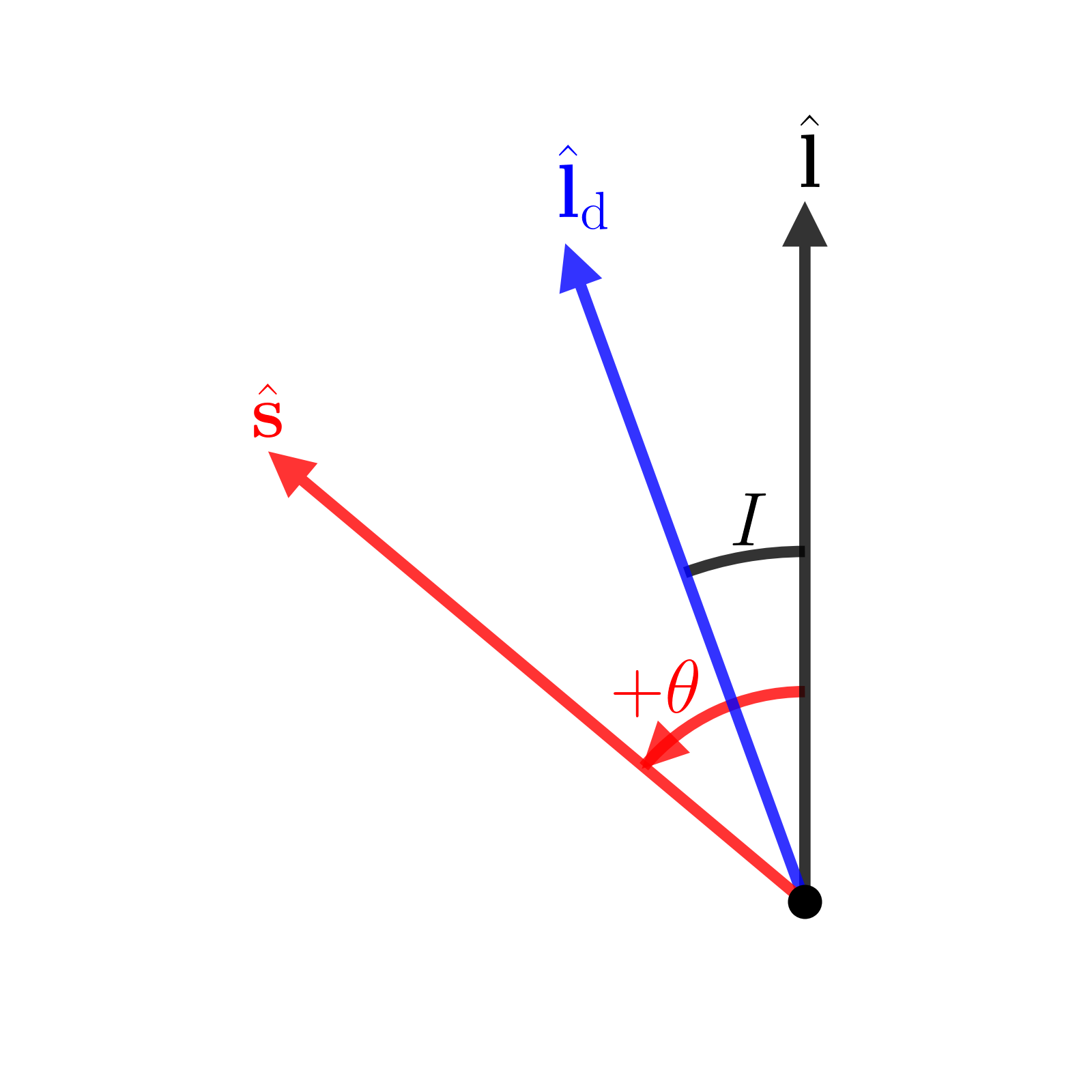
Figure 1: Definition of angles in the Cassini state configuration and the adopted sign convention for $\theta$. Traditionally, $\theta\in[-\pi,\pi]$.

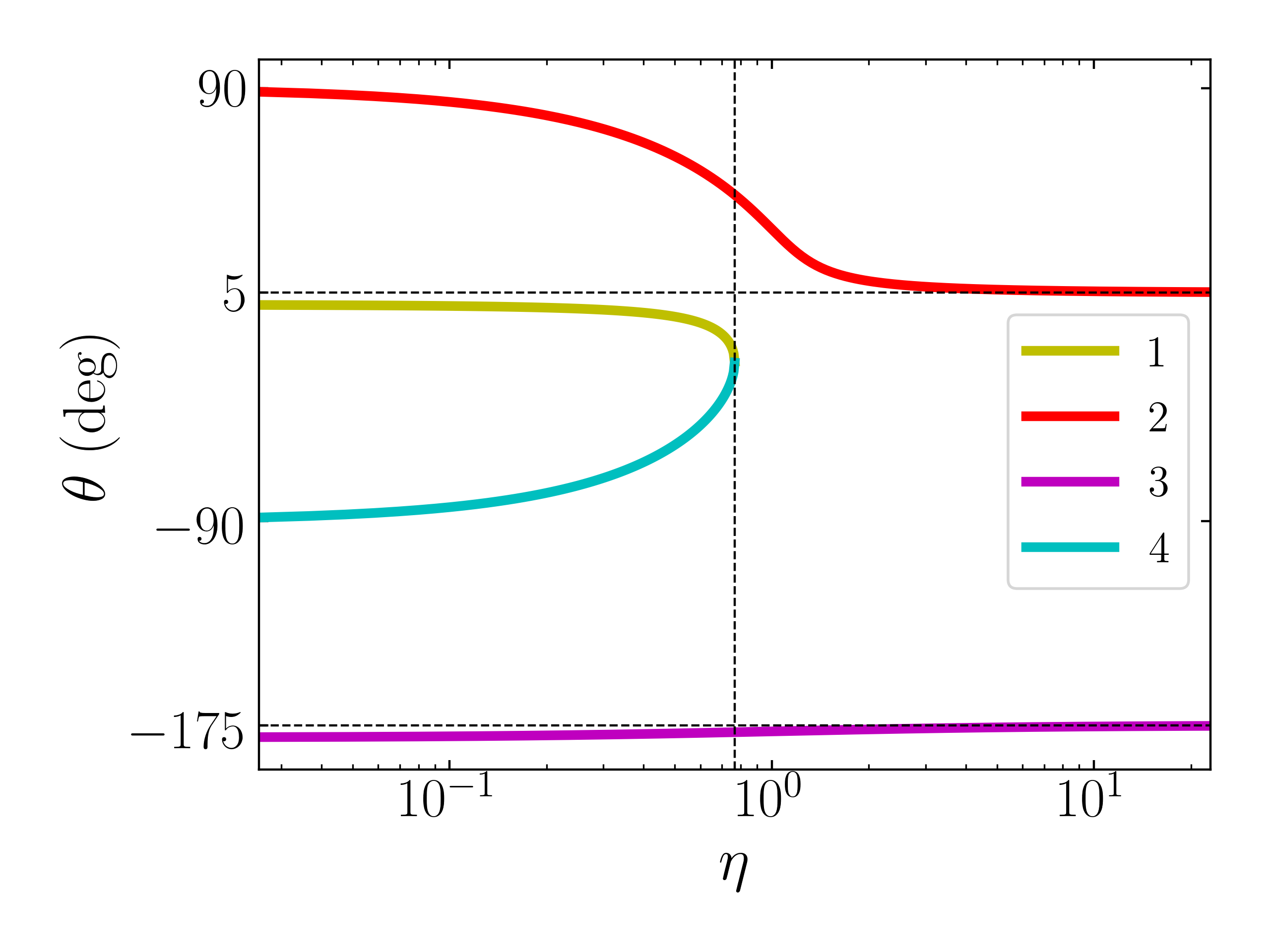
Figure 2: Cassini state obliquities as a function of $\eta$ for $I=5^{\circ}$. The thin vertical dashed line indicates $\eta_{\rm c}$ ($=0.766$ for $I=5^{\circ}$), where CS1 and CS4 merge and annihilate, and the thin horizontal dashed lines indicate $\theta=I$ and $I-180^{\circ}$, the asymptotic values for CSs 2 and 3 for $\eta\gg\eta_{\rm c}$.

Of the four CSs, 1, 2, 3 are stable while 4 is unstable. Appendix A gives the libration frequencies and growth rates, respectively, near these CSs.

2.3 Separatrix

The Hamiltonian (in the rotating frame) of the system is

$$\mathcal{H}\left(\phi,\cos\theta\right) =-\frac{1}{2}\left(\hat{\boldsymbol{\mathbf{s}}}\cdot\hat{\boldsymbol{\mathbf{l}}}\right)^{2}+\eta\left(\hat{\boldsymbol{\mathbf{s}}}\cdot\hat{\boldsymbol{\mathbf{l}}}_{\rm d}\right)$$

$$=-\frac{1}{2}\cos^{2}\theta+\eta\left(\cos\theta\cos I-\sin I\sin\theta\cos\phi\right).$$ (15)

Here, $\phi$ and $\cos\theta$ are canonically conjugate variables. Trajectories in the phase space $\left(\phi,\cos\theta\right)$ satisfy $H=$ constant (see Fig. 3).

When $\eta<\eta_{\rm c}$, CS4 exists and is a saddle point. The two trajectories originating and ending at CS4 are the only two infinite-period orbits in the phase space. Together, these two critical trajectories are referred to as the separatrix and divide phase space into three zones. In Fig. 3, we show the separatrix, the three zones, and their relations to the CSs. Trajectories in zone II librate about CS2 while those in zones I and III circulate.

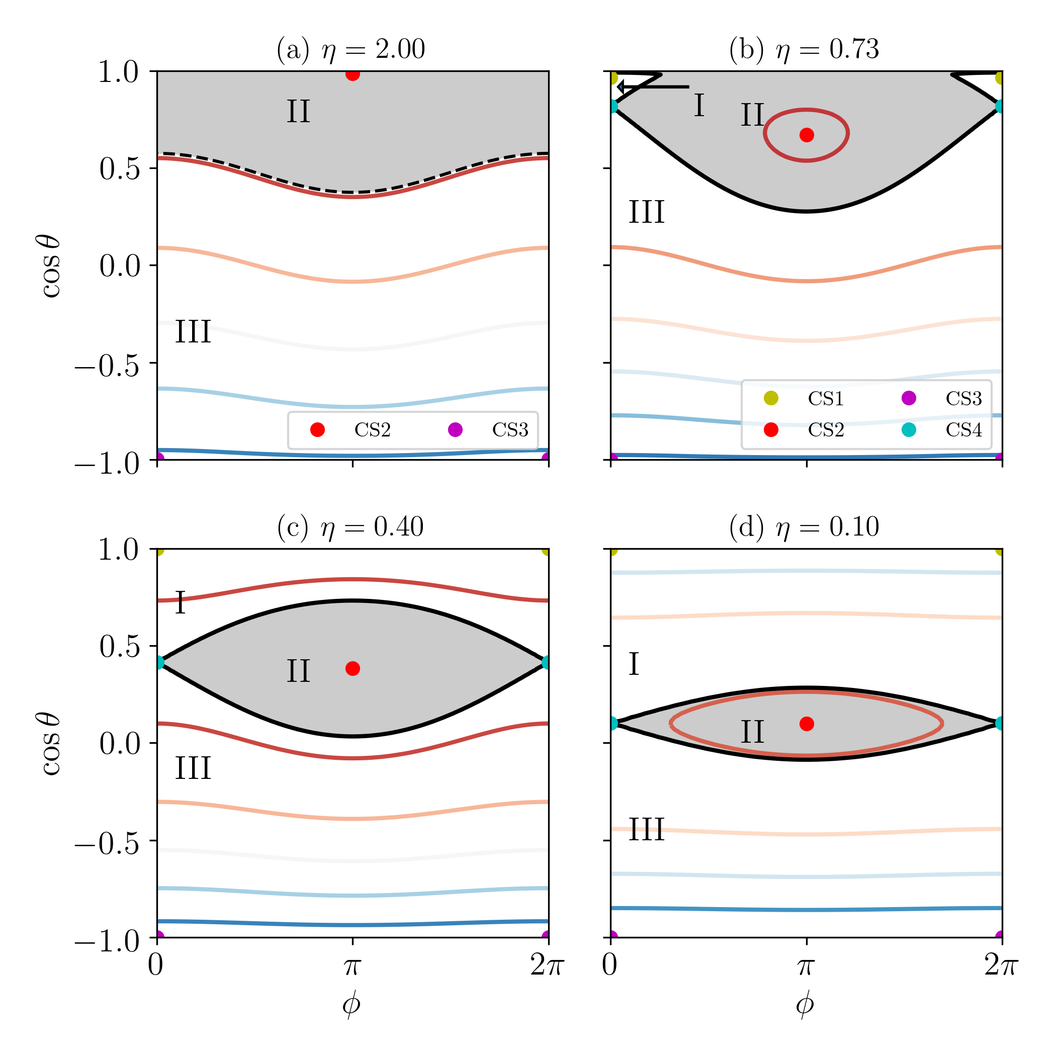
Figure 3: Level curves of $\mathcal{H}\left(\phi,\cos\theta\right)$ [Eq. (15)] for $I=5^{\circ}$, where warmer colors denote more positive values. The black solid line is the separatrix, which only exists for $\eta<\eta_{\rm c}=0.766$. The three zones (I, II, III), divided by the separatrix, are labeled. The Cassini states are denoted by filled circles and have the same colors as in Fig. 2. The interior of the separatrix, shaded in grey, is formally only defined for $\eta<\eta_{\rm c}$, but we may identify the points in phase space that flow into zone II when evolved forward in time (decreasing $\eta$ adiabatically); this is the shaded region in panel (a), bounded by the black dotted line.

Since $\left(\phi,\cos\theta\right)$ are canonically conjugate, the integral $\oint\cos\theta\;\mathrm{d}\phi$ along a trajectory is an adiabatic invariant (see Section 3). The unsigned areas $\left(\left|\int\cos\theta\;\mathrm{d}\phi\right|\right)$ of the three zones (as defined in Fig. 3) can be computed analytically. If we define

$$z_{0} =\eta\cos I, \chi =\sqrt{-\frac{\tan^{3}\theta_{4}}{\tan I}-1},$$ (16a)

$$\rho =\chi\frac{\sin^{2}\theta_{4}\cos\theta_{4}}{\chi^{2}\cos^{2}\theta_{4}+1}, T =2\chi\frac{\cos\theta_{4}}{\chi^{2}\cos^{2}\theta_{4}-1},$$ (16b)

then the areas for $\eta<\eta_{\rm c}$ are given by (Ward & Hamilton, 2004)

$$\mathcal{A}_{\rm I} =2\pi\left(1-z_{0}\right)-\frac{\mathcal{A}_{\rm II}}{2},$$ (17a)

$$\mathcal{A}_{\rm II} =8\rho+4\arctan T-8z_{0}\arctan\frac{1}{\chi},$$ (17b)

$$\mathcal{A}_{\rm III} =2\pi\left(1+z_{0}\right)-\frac{\mathcal{A}_{\rm II}}{2}.$$ (17c)

These are plotted as a function of $\eta$ in Fig. 4. While the zones are not formally defined for $\eta>\eta_{\rm c}$ since the separatrix disappears, a natural extension exists: evolve an initial phase space point $p$ under adiabatic decrease of $\eta$ until the separatrix appears at $\eta=\eta_{\rm c}$, then identify $p$ with the zone it is in at $\eta_{\rm c}$. Since phase space area is conserved under adiabatic evolution, this extension implies $\mathcal{A}_{\rm j}\left(\eta>\eta_{\rm c}\right)=\mathcal{A}_{\rm j}(\eta_{\rm c})$. The boundary between these extended zones is denoted by the dashed black line in panel (a) of Fig. 3, where no separatrix exists.

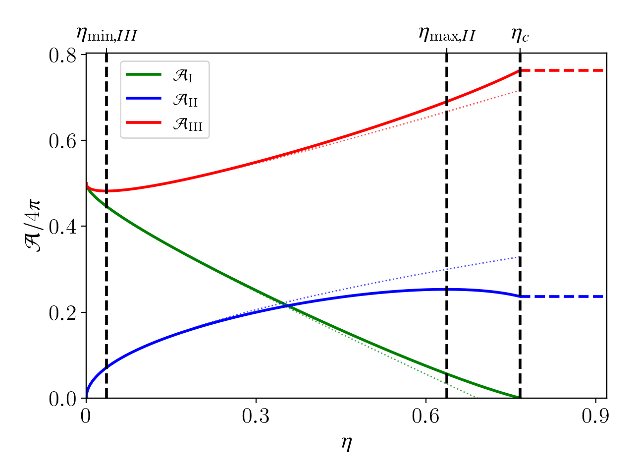
Figure 4: Plot of fractional areas of each of the zones $\mathcal{A}_{\rm j}(\eta)/4\pi$ as given by Eqs. (17) for $I=5^{\circ}$. The colored dotted lines correspond to small $\eta$ approximations used in Appendix B. The colored dashed lines for $\eta>\eta_{\rm c}$ are the effective values of $\mathcal{A}_{\rm II},\mathcal{A}_{\rm III}$ for $\eta>\eta_{\rm c}$, denoting the points that would flow into either area under adiabatic decrease of $\eta$ from $\eta>\eta_{\rm c}$ (see the text). The vertical black dashed lines correspond to $\eta=\eta_{\rm c}$ [Eq.(14)] and the values of $\eta$ for which $\mathcal{A}_{\rm II}$ is maximized ($\eta_{\rm\max,II}$) and for which $\mathcal{A}_{\rm III}$ is minimized ($\eta_{\rm\min,III}$, Eq. (30)).

3 Adiabatic Evolution

In this section, we study the evolution of the planetary obliquity $\theta$ when the parameter $\eta$ [or the disk mass $M_{\rm d}$; see Eqs. (8) and (11)] decreases sufficiently slowly that the evolution is adiabatic. Intuitively, this requires the disk evolution time $t_{\rm d}$ [Eq. (10)] be much larger than the spin precession period, $2\pi/\alpha$, i.e. $\epsilon=1/(\alpha t_{\rm d})\ll 1/(2\pi)$.

More rigorously, adiabaticity requires $t_{\rm d}$ be much larger than all timescales of the dynamical system governed by the Hamiltonian [Eq. (15)]. This is of course not possible in all cases, as the motion along the separatrix has an infinite period. In practice, as $\eta$ evolves, the system only crosses the separatrix once or twice, while it spends many orbits inside one of the three zones and far from the separatrix. Thus, a weak adiabaticity criterion is that, for all equilibria/fixed points, the local circulation/libration periods are much shorter than the timescale for the motion of the equilibria due to changing $\eta$. If this criterion is satisfied, then the system will evolve adiabatically for most of its evolution save one or two separatrix crossings.

As shown in Appendix A.2, libration about CS2 is slower than that about CS1 or CS3. As such, it has the smallest characteristic frequency in the system. The weak adiabaticity criterion is equivalent to requiring that, at all times other than separatrix crossing, the obliquity of CS2 ($\theta_{2}$) evolve over a longer timescale than the local libration period about CS2, i.e.

$$\left|\frac{\mathrm{d}\theta_{2}}{\mathrm{d}\tau}\right|\ll\frac{\omega_{\rm lib}}{2\pi},$$ (18)

where

$$\omega_{\rm lib}=\sqrt{\eta\sin I\sin\theta_{2}\left(1+\eta\sin I\csc^{3}\theta_{2}\right)},$$ (19)

is the libration frequency about CS2 for a given $\eta$ (Appendix A.2). This formula differs from that given in Millholland & Batygin (2019), where the $\csc^{3}\!\theta_{2}$ term is neglected and the square root is missing. Differentiating Eq. (13) gives

$$\frac{\mathrm{d}\theta_{2}}{\mathrm{d}\tau}=-\epsilon\frac{\eta\sin\left(\theta_{2}-I\right)}{\cos\left(2\theta_{2}\right)-\eta\cos\left(\theta_{2}-I\right)},$$ (20)

where $\epsilon=-\mathrm{d}(\ln\eta)/\mathrm{d}\tau$ [Eq. (12)]. Eq. (18) is most constraining at $\eta\sim 1$, i.e. it will be satisfied for all $\eta$ if it is satisfied near $\eta\sim 1$, where $\left|\mathrm{d}\theta_{2}/\mathrm{d}\tau\right|\sim\epsilon$. Thus, weak adiabiticity requires

$$\epsilon\ll\epsilon_{\rm c}\equiv\left(\frac{\omega_{\rm lib}}{2\pi}\right)_{\eta=1}\simeq\frac{1}{2\pi\sqrt{2}}\sqrt{\sin I\left(1+8\sin I\right)},$$ (21)

where in the last equality we have used $\sin\theta_{\rm 2}\simeq 1/2$ at $\eta=1$ (e.g. when $I=5^{\circ}$ and $\eta=1$, $\theta_{\rm 2}\approx 31^{\circ}$). For $I=5^{\circ}$, we obtain $\epsilon_{\rm c}\approx 0.0433$. Since our criterion is only a weak condition for adiabaticity, we use $\epsilon=3\times 10^{-4}$ in our “adiabatic” calculations below. We explore the consequences of nonadiabatic evolution in Section 4.

3.1 Adiabatic Evolution Outcomes

We consider the evolution of a system with arbitrary initial spin-disk misalignment angle $\theta_{\rm sd,i}$ and initial $\eta_{\rm i}\gg 1$. We are interested in the final spin obliquities $\theta_{\rm f}$ after $\eta$ gradually decreases to $\eta_{\rm f}\ll 1$ (i.e. after the disk has dissipated to a negligible mass). Note that when $\eta_{\rm i}\gg 1$, $\hat{\boldsymbol{\mathbf{l}}}$ precesses around $\hat{\boldsymbol{\mathbf{l}}}_{\rm d}$ much faster than the spin-orbit precession ($\left|\omega_{\rm ld}\right|\gg\left|\omega_{\rm sl}\right|$), and the spin obliquity $\theta$ varies rapidly. It is thus more appropriate to use $\theta_{\rm sd,i}$ rather than $\theta$ to specify the initial spin orientation. We explore the entire range $\theta_{\rm sd,i}\in[0,\pi]$ and choose $\epsilon=3\times 10^{-4}$ (see above).

To obtain the distribution of the final obliquities $\theta_{\rm f}$, we evenly sample $101$ values of $\theta_{\rm sd,i}$, and for each $\theta_{\rm sd,i}$ value, we pick $101$ evenly spaced orientations of $\hat{\boldsymbol{\mathbf{s}}}$ approximately from the ring of initial conditions having angular distance $\theta_{\rm sd,i}$ to $\hat{\boldsymbol{\mathbf{l}}}_{\rm d}$. To be concrete, we choose $\eta_{\rm i}=10\eta_{\rm c}$ where $\eta_{\rm c}$ is given by Eq. (14) and evolve Eqs. (9) and (11) until $\eta$ reaches its final value $10^{-5}$. At such a small $\eta$, $\hat{\boldsymbol{\mathbf{s}}}$ is strongly coupled to $\hat{\boldsymbol{\mathbf{l}}}$ and the final obliquity $\theta_{\rm f}$ is frozen. The mapping between $\theta_{\rm sd,i}$ and $\theta_{\rm f}$ is our primary result, and is shown for $I=5^{\circ}$, $10^{\circ}$, and $20^{\circ}$ in Figs. 5 and 6 respectively. The blue dots represent the results of the numerical calculation. The colored tracks are calculated semi-analytically using the method discussed in the following subsection.

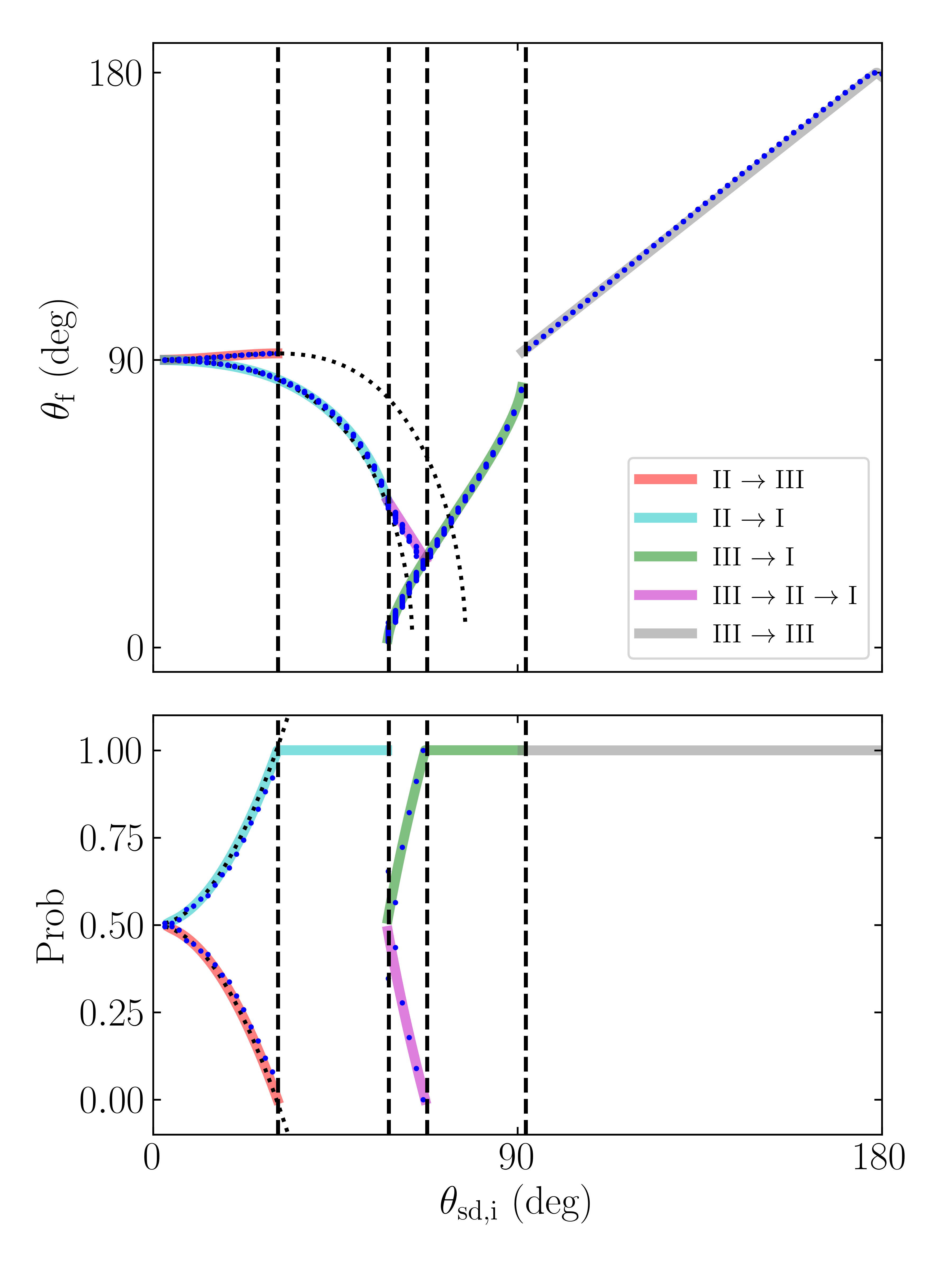
Figure 5: Top: The final spin obliquity $\theta_{\rm f}$ as a function of the initial spin-disk misalignment angle $\theta_{\rm sd,i}$ for systems evolving from initial $\eta_{\rm i}\gg 1$ to $\eta_{\rm f}\ll 1$, for $I=5^{\circ}$. The blue dots are results of numerical calculations (Section 3.1), and the colored tracks are semi-analytical results (Section 3.2). Bottom: The probabilities of different outcomes. Where a particular $\theta_{\rm sd,i}$ corresponds to multiple tracks, the system evolves probabilistically. The track that a particular system evolves along in a numerical simulation can be measured by examining its final obliquity. The dots represent the inferred probabilities from measured final obliquities in our simulations, while the colored tracks denote the semi-analytic probability of the system evolving along each track. There are five regimes of $\theta_{\rm sd,i}$ values for which different tracks are accessible. In both plots, the vertical dashed black lines denote semi-analytical calculations of the boundaries of these regimes (see Section 3.2), while the black dotted lines represent analytical approximations valid in the small-$\theta_{\rm sd,i}$ limit (see Appendix B).

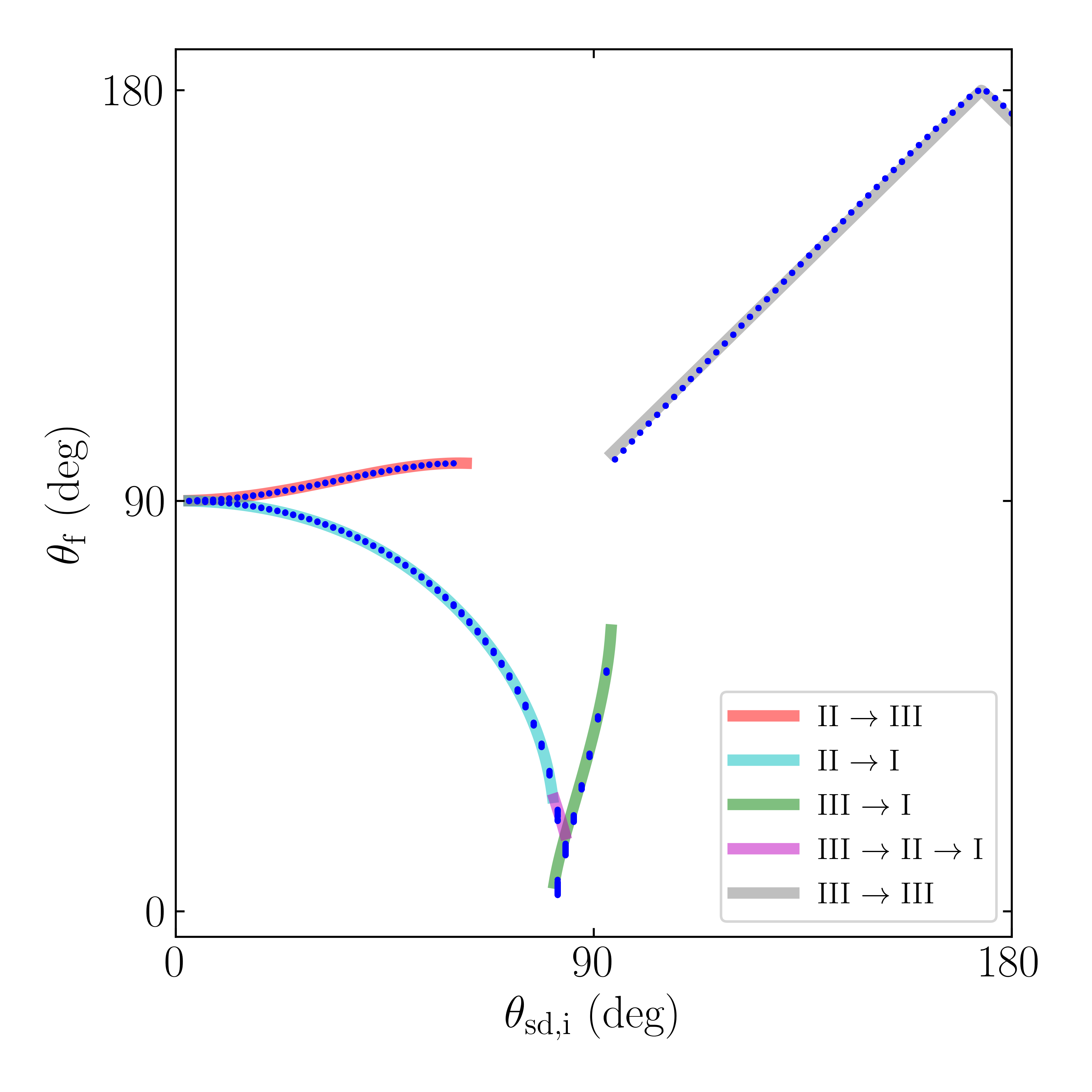
Figure 6: Same as the top panel of Fig. 5 but for $I=20^{\circ}$ and with fewer annotations.

3.2 Analytical Theory for Adiabatic Evolution

The evolutionary tracks that govern the $\theta_{\rm f}$-$\theta_{\rm sd,i}$ mapping correspond to various sequences of separatrix crossings. They can be understood using the principle of adiabatic invariance, combined with (i) how the enclosed phase space area by the trajectory evolves across each separatrix crossing, and (ii) the associated probabilities with each separatrix crossing.

3.2.1 Governing Principle: Evolution of Enclosed Phase Space Area

First, we consider how the enclosed phase space area by a trajectory evolves over time. In the absence of separatrix encounters, the enclosed phase space area $\oint\cos\theta\;\mathrm{d}\phi$ is an adiabatic invariant. We adopt convention where

$$A\equiv\oint\left(1-\cos\theta\right)\;\mathrm{d}\phi.$$ (22)

Note that $A$ can be negative when $\mathrm{d}\phi/\mathrm{d}t<0$, unlike the unsigned areas $\mathcal{A}_{\rm i}$ [Eqs. (17)] which are positive by definition. This definition of $A$ has two advantages: (i) it is continuous across transitions from circulating to librating that cross the North pole ($\cos\theta=1$), and (ii) the areas of the three zones are equal in absolute value to the expressions given in Eqs. (17). The path over which the integral is taken is either a libration or circulation cycle. When $\eta_{\rm i}\gg 1$, trajectories librate about $\hat{\boldsymbol{\mathbf{l}}}_{\rm d}$ with constant $\theta_{\rm sd}$, meaning they enclose initial phase space area

$$A_{\rm i}=2\pi\left(1-\cos\theta_{\rm sd,i}\right).$$ (23)

Complications arise when considering finite $\eta_{\rm i}$, as trajectories near CS2 or CS3 librate about these equilibria, rather than $\hat{\boldsymbol{\mathbf{l}}}_{\rm d}$, and Eq. (23) is no longer exact. In practice, Eq. (23) holds very well when defining $\theta_{\rm sd,i}$ as the angular distance to CS2; an exception is discussed in Section 3.2.3.

Beginning at the last separatrix crossing, the final enclosed phase space area $A_{\rm f}$ will be conserved for all time. As $\eta\to 0$, trajectories circulate about $\hat{\boldsymbol{\mathbf{l}}}$ at constant obliquity $\theta_{\rm f}$, related to $A_{\rm f}$ by

$$2\pi\left(1-\cos\theta_{\rm f}\right)=A_{\rm f}.$$ (24)

The enclosed phase space area is not conserved when the trajectory encounters the separatrix. However, the change is easily understood (Henrard, 1982). In essence, when the trajectory crosses the separatrix, it continues to evolve adjacent to the separatrix. So if a separatrix crossing results in a zone I trajectory (see Fig. 3), the new area can be approximated by integrating Eq. (22) along the upper leg of the separatrix. Pictorially, this can be seen in the bottom panels of Fig. 7.

3.2.2 Governing Principle: Probabilistic Separatrix Crossing

When a trajectory experiences separatrix crossing, it transitions into nearby zones probabilistically. This process is studied in the adiabatic limit by Henrard (1982) and Henrard & Murigande (1987). Their results may be summarized as follows: if zone $i$ is shrinking while adjacent zones $j,k$ are expanding such that the sum of their areas is constant, the probabilities of transition from zone $i$ to zones $j$ and $k$ are given by

$$\Pr\left(i\to j\right)=-\frac{\partial\mathcal{A}_{\rm j}/\partial\eta}{\partial\mathcal{A}_{\rm i}/\partial\eta},$$ (25a)

$$\Pr\left(i\to k\right)=-\frac{\partial\mathcal{A}_{\rm k}/\partial\eta}{\partial\mathcal{A}_{\rm i}/\partial\eta}.$$ (25b)

Note that $\Pr\left(i\to j\right)+\Pr\left(i\to k\right)=1$. Eqs. (25) can be used in conjunction with Eqs. (17) to understand for what initial conditions each track can be observed and with what probabilities.

As an example, consider a system in zone II in panel (d) of Fig. 3. As $\eta$ decreases, zone II will shrink while zones I and III will expand until the trajectory crosses the separatrix. Suppose the trajectory exits zone II at some $\eta_{\star}$, then the probability of the II $\to$ I transition is $\Pr\left(\rm II\to I\right)=-\dot{A}_{\rm I}/\dot{A}_{\rm II}$, while the II $\to$ III transition occurs with probability $\Pr\left(\rm II\to III\right)=-\dot{A}_{\rm III}/\dot{A}_{\rm II}$.

3.2.3 Evolutionary Trajectories

Returning to the evolution of $\hat{\boldsymbol{\mathbf{s}}}$, we can classify trajectories by the sequence of separatrix encounters. Initially, in the $\eta>\eta_{\rm c}$ regime, only zones II and III exist; as $\eta\to 0$, only zones I and III exist (see Fig. 3). There are five distinct evolutionary tracks:

1. II $\to$ I (see Fig. 7 for an example). The spin axis $\hat{\boldsymbol{\mathbf{s}}}$ initially circulates in zone II (snapshot a), and then starts librating about CS2 as $\eta$ decreases (snapshot b), enclosing some initial phase space area $A_{\rm i}$. This libration continues until the separatrix expands (due to decreasing $\eta$) to “touch” the trajectory (snapshot c), at which $\mathcal{A}_{\rm II}(\eta_{\star})=A_{\rm i}$. As $\hat{s}$ moves to a circulating trajectory in zone I immediately bordering the separatrix, it will encompass $-\mathcal{A}_{\rm I}(\eta_{\star})$ phase space area. The final obliquity $\theta_{\rm f}$ is then given by Eq. (24), with $A_{\rm f}=-\mathcal{A}_{\rm I}\left(\eta_{\star}\right)$. An analytical approximation to $\theta_{\rm f}$ is derived in Appendix B and is

   $$\left(\cos\theta_{\rm f}\right)_{\rm II\to I}\simeq\left(\frac{\pi\theta_{\rm sd,i}^{2}}{16}\right)^{2}\cot I+\frac{\theta_{\rm sd,i}^{2}}{4}.$$ (26)

   The transition probability is

   $$\Pr\left(\mathrm{II}\to\mathrm{I}\right)=-\left(\frac{\partial\mathcal{A}_{\rm I}/\partial\eta}{\partial\mathcal{A}_{\rm II}/\partial\eta}\right)_{\eta=\eta_{\star}}.$$ (27)

   This track can only occur when the initial condition begins in zone II, requiring $A_{\rm i}<\mathcal{A}_{\rm II}(\eta_{\rm c})$, where $\mathcal{A}_{\rm II}\left(\eta_{c}\right)$ is given by Eq. (17b) evaluated at $\eta=\eta_{c}$. Since $\partial\mathcal{A}_{\rm I}/\partial\eta<0$ everywhere, while $\partial\mathcal{A}_{\rm II}/\partial\eta>0$ at all possible $\eta_{\star}$ for an initial condition starting in zone II, this track always has nonzero probability.

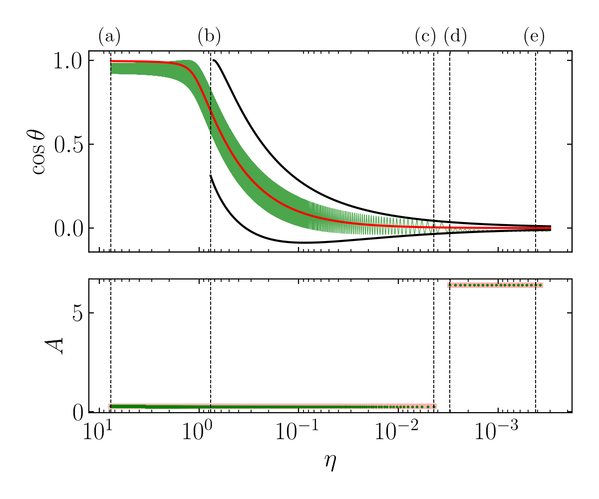
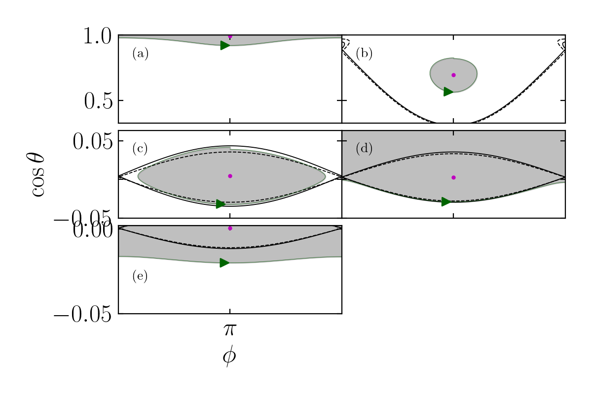
Figure 8: Same as Fig. 7 but for the II $\to$ III track. $\theta_{\rm sd,i}=17.2^{\circ}$ and $\epsilon=3.01\times 10^{-4}$.

2. II $\to$ III (see Fig. 8). This track is similar to the II $\to$ I track; the only difference is that, upon separatrix encounter, the trajectory follows the circulating trajectory in zone III bordering the separatrix, upon which it will encompass area $\mathcal{A}_{\rm I}(\eta_{\star})+\mathcal{A}_{\rm II}(\eta_{\star})=A_{\rm f}$. The final obliquity is still given by Eq. (24), and the analytical approximation derived in Appendix B is

   $$\left(\cos\theta_{\rm f}\right)_{\rm II\to III}\simeq\left(\frac{\pi\theta_{\rm sd,i}^{2}}{16}\right)^{2}\cot I-\frac{\theta_{\rm sd,i}^{2}}{4}.$$ (28)

   The transition probability is

   $$\Pr\left(\mathrm{II}\to\mathrm{III}\right)=-\left(\frac{\partial\mathcal{A}_{\rm III}/\partial\eta}{\partial\mathcal{A}_{\rm II}/\partial\eta}\right)_{\eta=\eta_{\star}}.$$ (29)

   Again, this track can only occur when $A_{\rm i}<\mathcal{A}_{\rm II}(\eta_{\rm c})$, but a further constraint arises when we consider the transition probability. Upon examination of Fig. 4, it is clear that $\partial\mathcal{A}_{\rm III}/\partial\eta>0$ for a large range of $\eta$, which would give a negative transition probability—implying a forbidden transition. Define

   $$\eta_{\min,III}\equiv\operatorname*{argmin}\mathcal{A}_{\rm III}(\eta),$$ (30)

   which is labeled in Fig. 4. Thus, the II $\to$ III track is permitted only if $\eta_{\star}<,\eta_{\rm\min,III}$.

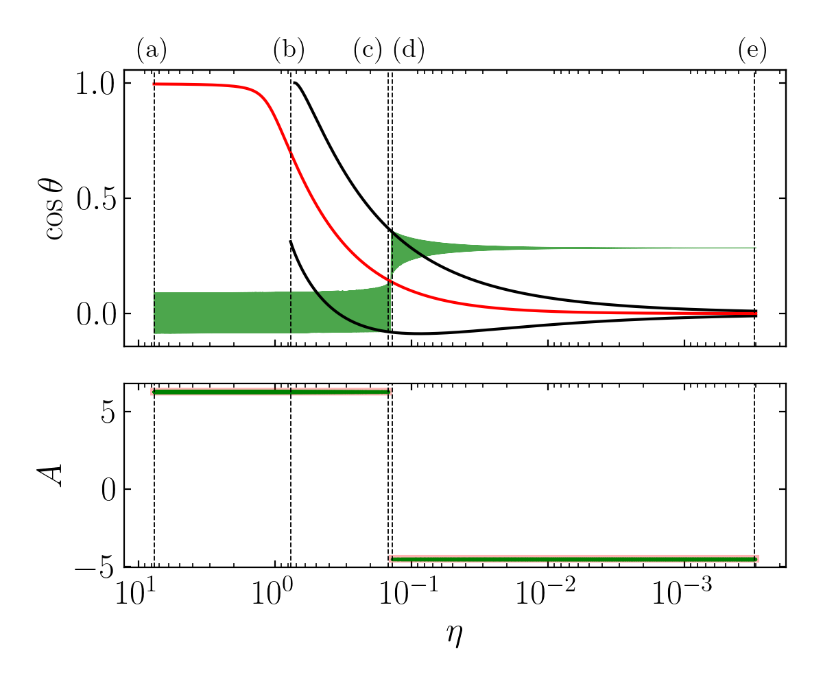
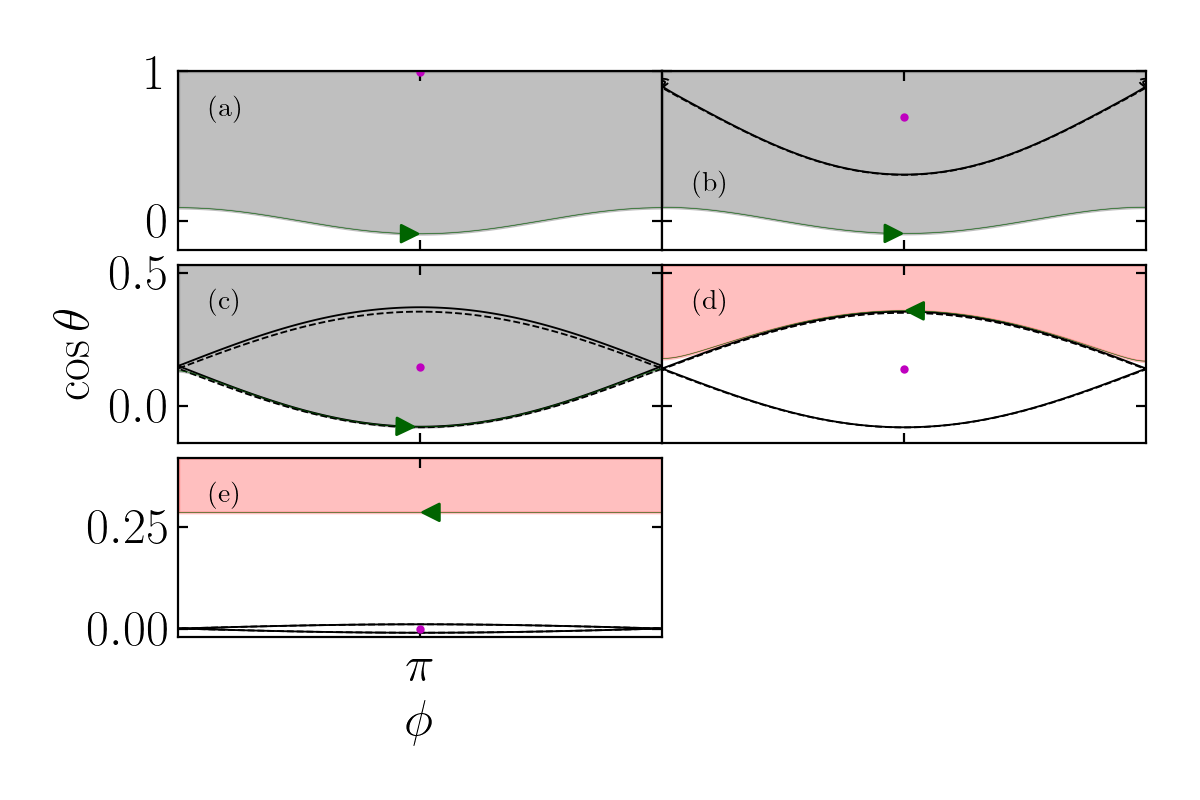
Figure 9: Same as Fig. 7 but for the III $\to$ I track. $\theta_{\rm sd,i}=89.1^{\circ}$, and $\epsilon=3\times 10^{-4}$.

3. III $\to$ I (see Fig. 9). The trajectory encounters the separatrix when $\mathcal{A}_{\rm I}(\eta_{\star})+\mathcal{A}_{\rm II}(\eta_{\star})=A_{\rm i}$, upon which it transitions to a zone I trajectory enclosing $A_{\rm f}=-\mathcal{A}_{\rm I}$. The final obliquity is again given by Eq. (24).

   This track can only occur if $A_{\rm i}>\mathcal{A}_{\rm II}(\eta_{\rm c})$, but is also constrained by requiring $A_{\rm i}$ be sufficiently small so that it will encounter the separatrix (if $A_{\rm i}$ is too large, it will never encounter the separatrix, and we simply have a III $\to$ III transition). This condition is $A_{\rm i}<\max\left(\mathcal{A}_{\rm I}+\mathcal{A}_{\rm II}\right)=4\pi-\min\left(\mathcal{A}_{\rm III}\right)$. Since $\partial\mathcal{A}_{\rm I}/\partial\eta<0$ and $\partial\mathcal{A}_{\rm III}/\partial\eta>0$ for all accessible $\eta_{\star}$, this track is always permitted.

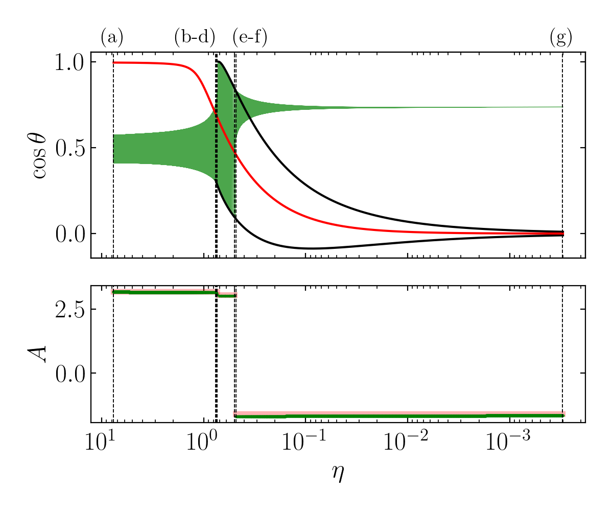
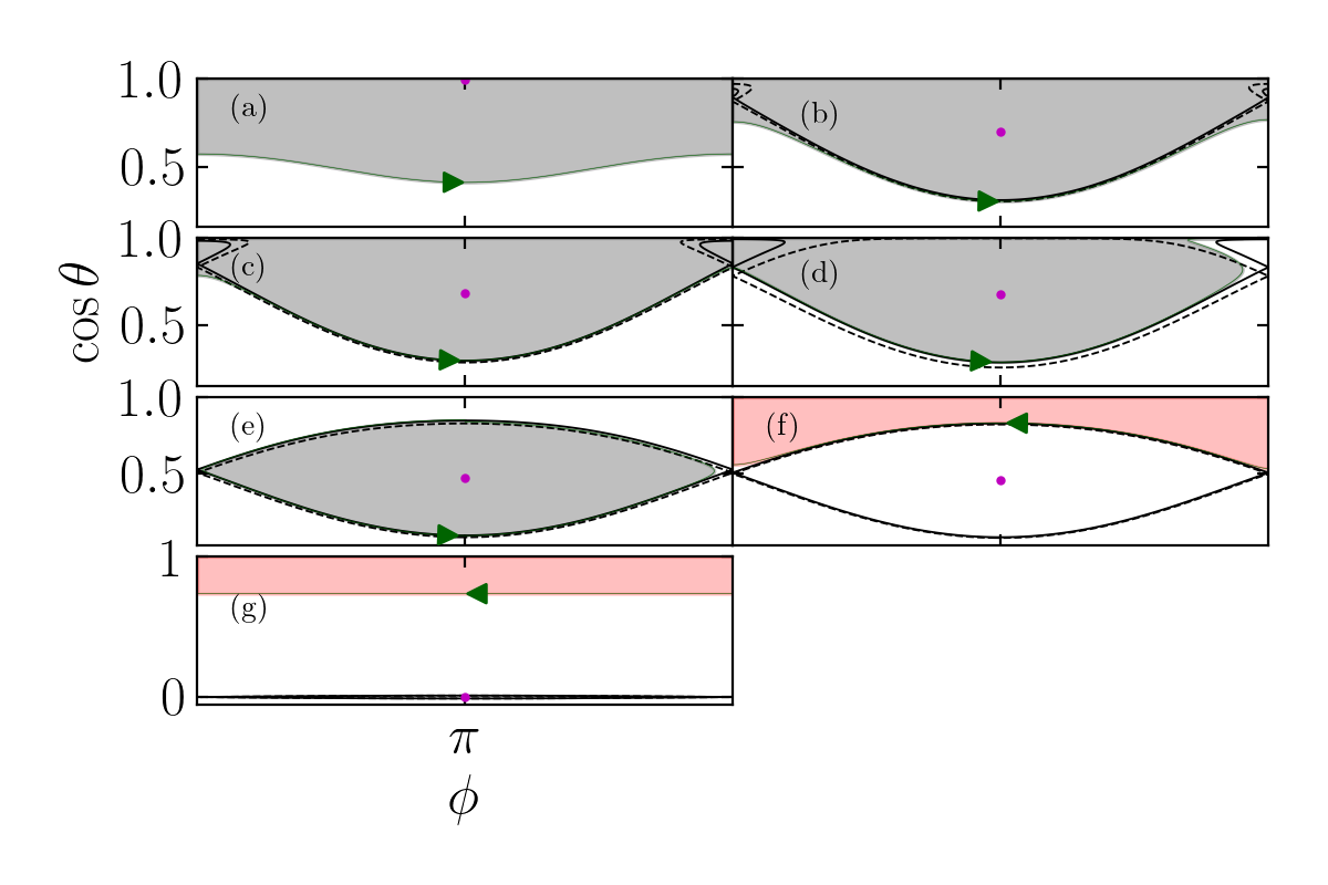
Figure 10: Same as Fig. 7 but for the III $\to$ II $\to$ I track. $\theta_{\rm sd,i}=60^{\circ}$, and $\epsilon=3.14\times 10^{-4}$. Two separatrix crossings are shown, in panels (c-d) and (e-f).

4. III $\to$ II $\to$ I (see Fig. 10). That $\mathcal{A}_{\rm II}(\eta)$ is not a monotonic function of $\eta$ (see Fig. 4) is key to the existence of this track. Consider a trajectory originating in zone III that first encounters the separatrix at $\eta_{1}$, when $\mathcal{A}_{\rm I}(\eta_{1})+\mathcal{A}_{\rm II}(\eta_{1})=A_{\rm i}$, such that it transitions into zone II enclosing intermediate phase space area $A_{\rm m}=\mathcal{A}_{\rm II}(\eta_{1})$. Such a transition has probability

   $$\Pr\left(\rm III\to II\right)=-\left(\frac{\partial\mathcal{A}_{\rm II}/\partial\eta}{\partial\mathcal{A}_{\rm III}/\partial\eta}\right)_{\eta=\eta_{1}},$$ (31)

   which is nonnegative (i.e. the transition is permitted) if $\eta_{1}\in[\eta_{\rm\max,II},\eta_{\rm c}]$. Equivalently, this requires $A_{\rm i}\in\left[\mathcal{A}_{\rm II}\left(\eta_{\rm c}\right),\mathcal{A}_{\rm II,\max}\right]$. Then, as $\eta$ continues to decrease, a second $\eta_{2}$ value exists for which $A_{\rm m}=\mathcal{A}_{\rm II}(\eta_{2})$, upon which the trajectory is ejected to zone I and $A_{\rm f}=-\mathcal{A}_{\rm I}(\eta_{2})$. Note that $\eta_{2}<\eta_{\rm\max,II}$ necessarily, as zone II must be shrinking in order for the trajectory to be ejected. The final obliquity is given by Eq. (24). Graphical inspection of Fig. 4 shows that $\partial\mathcal{A}_{\rm II}/\partial\eta$ and $\partial\mathcal{A}_{\rm III}/\partial\eta$ have the same signs for $\eta<\eta_{\rm\max,II}$, and therefore the complementary II $\to$ I transition is guaranteed. Overall, the III $\to$ II $\to$ I track is permitted so long as the first transition is permitted, or $A_{\rm i}\in\left[\mathcal{A}_{\rm II}\left(\eta_{\rm c}\right),\mathcal{A}_{\rm II,\max}\right]$.

5. III $\to$ III. This track is the trivial case where no separatrix encounter occurs, and $A$ is constant throughout the evolution ($A_{\rm f}=A_{\rm i}$) except for a jump by $4\pi$ when crossing the South pole ($\cos\theta=-1$) due to the coordinate singularity. This requires $A_{\rm i}>\max\left(\mathcal{A}_{\rm I}+\mathcal{A}_{\rm II}\right)$. In the limit of $\eta_{\rm i}\to\infty$ and $\eta_{\rm f}\to 0$ we have $\theta_{\rm f}=\theta_{\rm sd,i}$. For finite $\eta_{\rm i}$, the initial enclosed phase space area for III $\to$ III trajectories is not given exactly by using $\theta=\theta_{\rm sd,i}$ in Eq. (23). This is because the initial orbits for such trajectories are better described as librating about CS3 with angle of libration $\Delta\theta-\theta_{\rm sd,i}$ rather than about CS2 with angle of libration $\theta_{\rm sd,i}$. Here, $\Delta\theta$ is the angular distance between CS2 and CS3 and is not equal to $180^{\circ}$ except when $\eta_{\rm i}\to\infty$. This finite-$\eta_{\rm i}$ effect is responsible for the small cusp at the very right ($\theta_{\rm sd,i}\to 180^{\circ}$) of Figs. 5 and 6.

In summary, starting from an initial condition with phase space area $A_{\rm i}$ at $\eta=\eta_{\rm i}\gg 1$, the five evolutionary tracks are:

1. $A_{\rm i}\in\left[0,\mathcal{A}_{\rm II}\left(\eta_{\rm\min,III}\right)\right]$: Both the II $\to$ III and the II $\to$ I tracks are possible.

2. $A_{\rm i}\in\left[\mathcal{A}_{\rm II}\left(\eta_{\rm\min,III}\right),\mathcal{A}_{\rm II}(\eta_{\rm c})\right]$: Only the II $\to$ I track.

3. $A_{\rm i}\in\left[\mathcal{A}_{\rm II}(\eta_{\rm c}),\mathcal{A}_{\rm II,\max}\right]$: Both the III $\to$ I and III $\to$ II $\to$ I are possible.

4. $A_{\rm i}\in\left[\mathcal{A}_{\rm II,\max},\max\left(\mathcal{A}_{\rm I}+\mathcal{A}_{\rm II}\right)\right]$: Only the III $\to$ I track.

5. $A_{\rm i}>\max\left(\mathcal{A}_{\rm I}+\mathcal{A}_{\rm II}\right)$: Only the III $\to$ III track.

In all cases, the corresponding ranges for $\theta_{\rm sd,i}$ can be computed via Eq. (23). The boundaries between these ranges are overplotted in Fig. 5, where they can be seen to agree well with the numerical results.

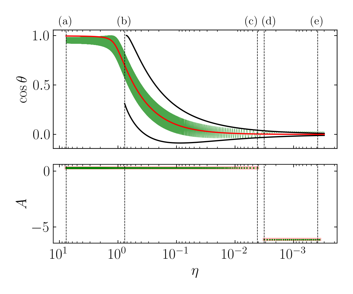
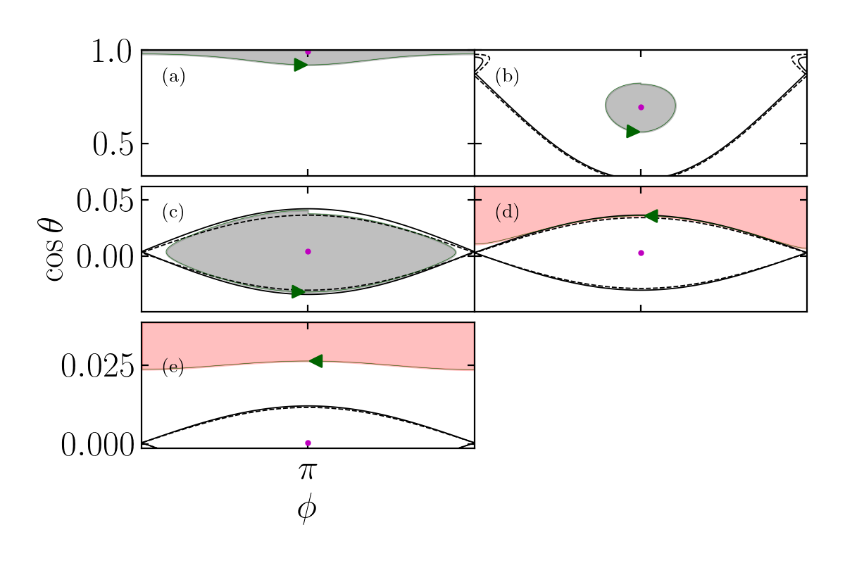
Figure 7: An example of the II $\to$ I evolutionary track for $I=5^{\circ}$ and $\theta_{\rm sd,i}=17.2^{\circ}$. Upper panel: The thin green line shows $\cos\theta$ as a function of $\eta$, obtained by numerical integration (with $\epsilon=3\times 10^{-4}$). Overlaid are the location of Cassini State 2 (dashed red) and the upper and lower bounds on the separatrix (dotted black). The trajectory tracks CS2 to a final obliquity of $88.57^{\circ}$. The black vertical dashed lines denote instants in the simulation portrayed in bottom panels. Middle panel: The enclosed separatrix area obtained by integrating the simulated trajectory (green dots) and adiabatic theory (red line). Lower plot: Snapshots in $\left(\cos\theta,\phi\right)$ phase space of one circulation/libration cycle of the trajectory, shown in dark green with an arrow indicating direction. The snapshots correspond to the start of the simulation (a), the appearance of the separatrix (b), two panels depicting the separatrix crossing process (c-d), and a final snapshot at $\eta=10^{-3.5}$ (e). The separatrices at the beginning and end of the portrayed cycle in each snapshot are shown in solid/dashed black lines respectively. Also labeled is CS2 at the start of each cycle (filled red circle). Finally, the enclosed phase space area is shaded in grey ($A>0$) and red ($A<0$).

4 Nonadiabatic Effects

In Section 3, we have examined the spin axis evolution in the limit where $\epsilon\ll\epsilon_{\rm c}$ [see Eq. (21)] and the evolution is mostly adiabatic (except at separatrix crossings). We now consider nonadiabatic effects.

4.1 Transition to Non-adiabaticity: Results for $\epsilon\lesssim\epsilon_{\rm c}$

To illustrate the transition to nonadiabaticity, we carried out a suite of numerical calculations for several values of $\epsilon$. The results for two of these values are shown in Figs. 11 and 12.

As $\epsilon$ increases (see Fig. 11), nonadiabaticity manifests as a larger scatter of final obliquities near the tracks predicted from adiabatic evolution. This scatter first sets in for trajectories starting in zone III, as these trajectories encounter the separatrix at larger $\eta$ compared to those originating in zone II. This means the obliquity of CS2 $\theta_{2}$ is smaller for these trajectories, and the adiabaticity criterion is stricter [see Eq. (21)]. Physically, approaching the adiabaticity criterion corresponds to the separatrix crossing process becoming sensitive to the phase of the libration/circulation cycle at the crossing: if the trajectory crosses the separatrix when the obliquity is at its maximum, the final obliquity will also be relatively larger.

As $\epsilon$ increases further (see Fig. 12) but still marginally satisfies the weak adiabaticity criterion [Eq. (21)], the scatter in $\theta_{\rm f}$ continues to widen. The horizontal banded structure of the final obliquities is a consequence of even stronger phase sensitivity during separatrix crossing: trajectories cross the separatrix at similar phases evolve to similar final obliquities that only depend weakly on on $\theta_{\rm sd,i}$. Finally, in Fig. 12, the bottom edge of the data and the III $\to$ I track deviate very noticeably. This non-adiabatic effect is the result of the separatrix evolving significantly within the separatrix-crossing orbit, as the tracks computed in Section 3 assume that $\eta$ is constant throughout the separatrix-crossing orbit.

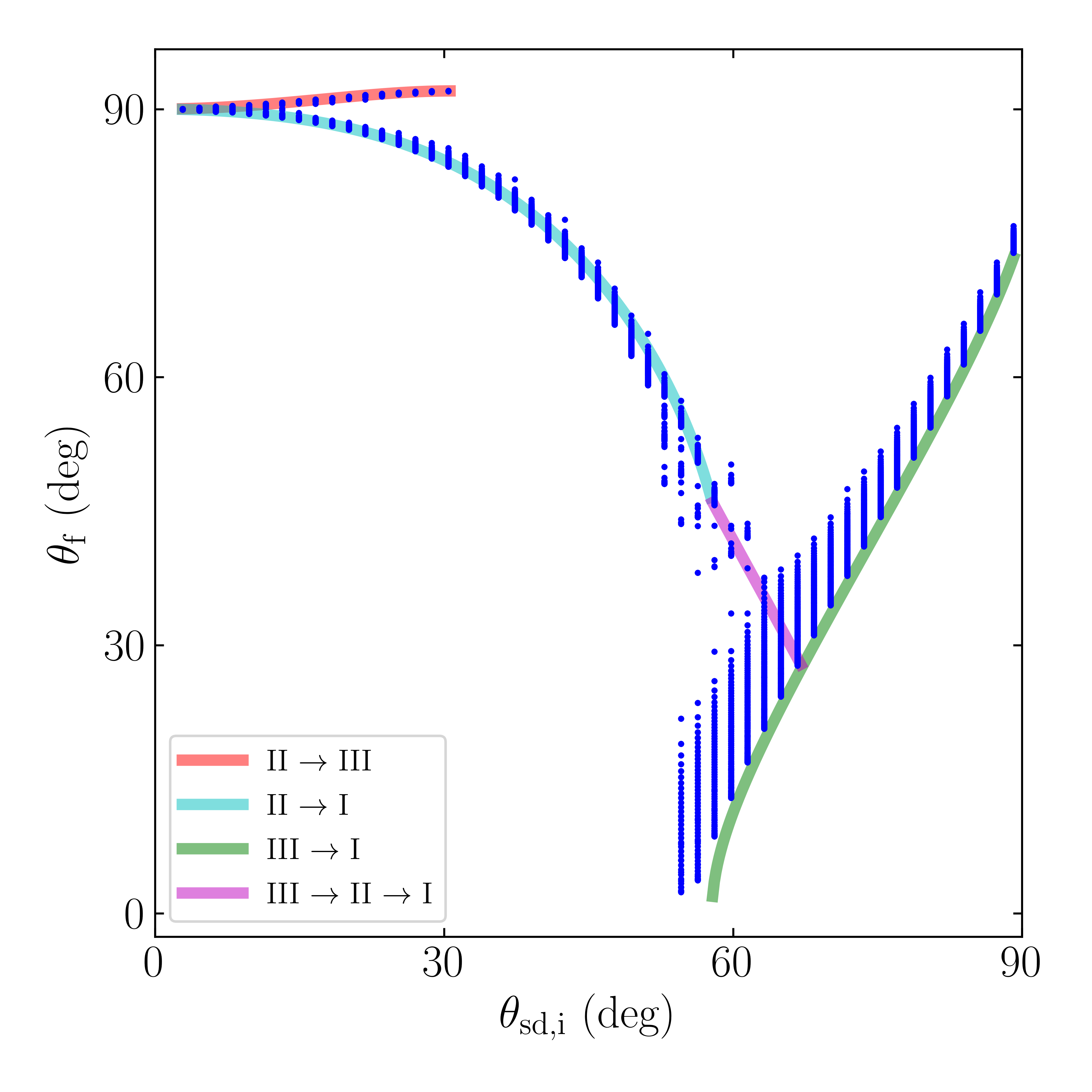
Figure 11: Same as Fig. 5 but for $\epsilon=10^{-2.5}$ and restricting $\theta_{\rm sd,i}<90^{\circ}$ (blue dots). The colored solid lines are analytical adiabatic results (same as shown in Fig. 5). A larger spread from the adiabatic tracks is observed in the numerical results due to the non-adiabaticity effect.

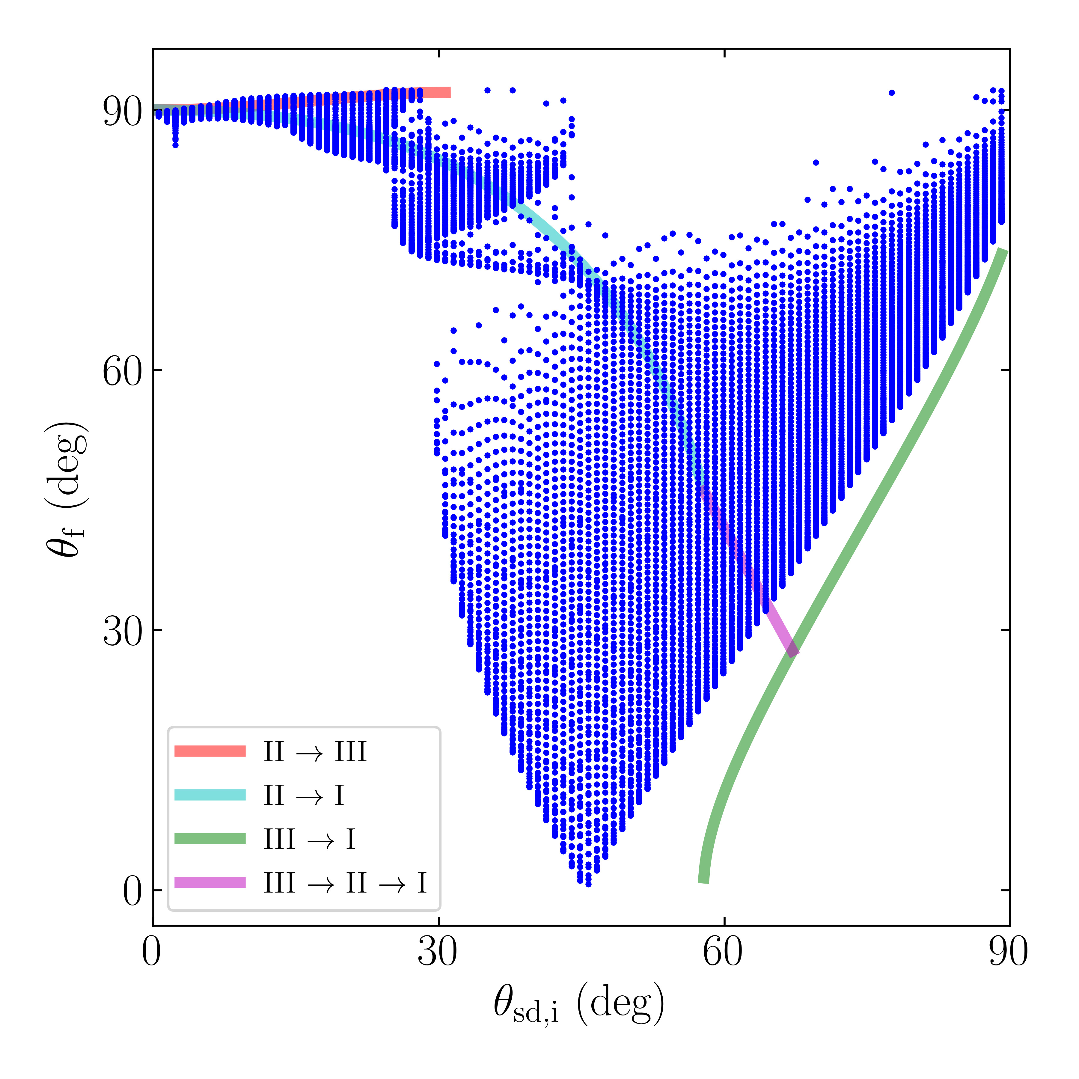
Figure 12: Same as Fig. 11 but for $\epsilon=10^{-1.5}$ (i.e. larger non-adiabaticity effect). Some small resemblance to the adiabatic tracks remains, and the deviations appear to have a banded structure.

A sample trajectory following in the style of Fig. 7 but for $\epsilon=0.3$ (violating even weak adiabaticity) is provided in Fig. 13. It is clear that the trajectory does not track the level curves of the Hamiltonian during each individual snapshot. This results from CS2 migrating more quickly than the trajectory can librate about CS2, violating the weak adiabaticity criterion.

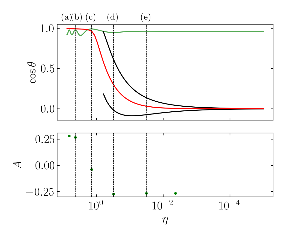
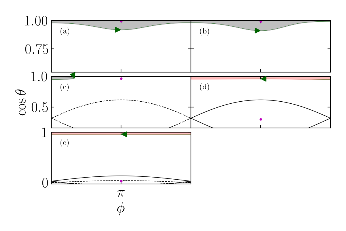
Figure 13: Same as Fig. 7 but for a nonadiabatic case, with $\epsilon=0.3$. In the top panel, it is evident that the libration cycle about CS2 is unable to keep up with the swift migration of CS2 as $\eta$ changes, decreasing the obliquity excitation compared to the adiabatic simulation. In the middle panel, the trajectory only undergoes six libration/circulation cycles before $\eta<10^{-5}$, and the enclosed phase space area is clearly not conserved. In the bottom panel, we can see that individual trajectories do not lie along level curves of the Hamiltonian, as the Hamiltonian phase space changes quickly compared to the period of circulation cycles.

4.2 Non-adiabatic Evolution: Result for $\epsilon\gtrsim\epsilon_{\rm c}$

In general, numerical calculations are needed to determine the non-adiabatic obliquity evolution ($\epsilon\gtrsim\epsilon_{\rm c}$). However, some analytical results can still be obtained when the obliquity change is small.

We start from Eq. (9), which governs the evolution of the spin axis in the rotating frame. We choose coordinate axes such that $\hat{\boldsymbol{\mathbf{l}}}=\hat{\boldsymbol{\mathbf{z}}}$ and $\hat{\boldsymbol{\mathbf{l}}}_{\rm d}=\hat{\boldsymbol{\mathbf{z}}}\cos I+\hat{\boldsymbol{\mathbf{x}}}\sin I$, giving

$$\left(\frac{\mathrm{d}\hat{\boldsymbol{\mathbf{s}}}}{\mathrm{d}\tau}\right)_{\rm rot}=\left[\left(\eta\cos I-\cos\theta\right)\hat{\boldsymbol{\mathbf{z}}}+\eta\sin I\,\hat{\boldsymbol{\mathbf{x}}}\right]\times\hat{\boldsymbol{\mathbf{s}}}.$$ (32)

Defining $S={\hat{s}}_{\rm x}+i{\hat{s}}_{\rm y}$, we find

$$\frac{\mathrm{d}S}{\mathrm{d}\tau}=i\left(\eta\cos I-\cos\theta\right)S-i\eta\sin I\cos\theta.$$ (33)

To proceed, we assume the obliquity is roughly constant, $\cos\theta\approx\cos\theta_{\rm i}$. Eq. (33) can then be solved explicitly, starting from the initial value $S(\tau_{\rm i})$:

$$S(\tau)e^{-i\Phi(\tau)}-S(\tau_{\rm i})\simeq-i\sin I\cos\theta_{\rm i}\int_{\tau_{\rm i}}^{\tau}\eta(\tau^{\prime})e^{-i\Phi(\tau^{\prime})}\;\mathrm{d}\tau^{\prime},$$ (34)

where

$$\Phi(\tau)\equiv\int_{\tau_{\rm i}}^{\tau}\left(\eta(\tau^{\prime})\cos I-\cos\theta_{\rm i}\right)\;\mathrm{d}\tau^{\prime}.$$ (35)

We now invoke the stationary phase approximation, so that $\Phi(\tau)\simeq\Phi(\tau_{0})+(1/2)\ddot{\Phi}(\tau_{0})(\tau-\tau_{0})^{2}$, where $\tau_{0}$ is determined by $\dot{\Phi}=0$, occurring when $\eta_{0}=\cos\theta_{i}/\cos I$. We then find, for $\tau\gg\tau_{0}$,

$$S(\tau)e^{-i\Phi(\tau)}-S(\tau_{\rm i})\simeq-i\eta(\tau_{0})\sin I\cos\theta_{\rm i}\,e^{-i\Phi(\tau_{0})}\sqrt{\frac{2\pi}{i\ddot{\Phi}(\tau_{0})}}.$$ (36)

Using $\dot{\eta}=-\epsilon\eta$ [Eq. (11)] and $\ddot{\Phi}(\tau_{0})=\dot{\eta}(\tau_{0})\cos I=-\epsilon\cos\theta_{i}$, we have

$$S(\tau)e^{-i\Phi(\tau)}-S(\tau_{\rm i})\simeq-i^{3/2}\tan I(\cos\theta_{\rm i})^{3/2}e^{-i\Phi(\tau_{0})}\sqrt{\frac{2\pi}{\epsilon}}.$$ (37)

The final obliquity $\theta_{\rm f}$ is then given by

$$\sin\theta_{\rm f}\simeq\left|\sin\theta_{i}+e^{-i\varphi_{0}}\tan I(\cos\theta_{\rm i})^{3/2}\sqrt{\frac{2\pi}{\epsilon}}\right|,$$ (38)

where $\varphi_{0}=\Phi(\tau_{0})+\pi/4$ is a constant phase. If the initial obliquity is much smaller than the final obliquity ($\sin\theta_{\rm i}\ll\sin\theta_{\rm f}$), we obtain

$$\sin\theta_{\rm f}\simeq\sqrt{\frac{2\pi}{\epsilon}}\tan I(\cos\theta_{\rm i})^{3/2}.$$ (39)

This expression is valid only if $\cos\theta\approx\cos\theta_{\rm i}$ throughout the evolution. This corresponds to the limit where $\theta_{\rm f}$ is not much larger than $\theta_{\rm i}$, which requires $\epsilon$ not to be too small. Numerically, this is consistent with the system being in the nonadiabatic regime $\epsilon\gtrsim\epsilon_{\rm c}$ (see Fig. 14).

The above calculation applies for a specific initial $\theta_{\rm i}$, but, as discussed at the beginning of Section 3.1, the initial spin orientation is more appropriately described by $\theta_{\rm sd,i}$ since $\eta_{i}\gg 1$. The correct way to predict the final obliquity for a given $\theta_{\rm sd,i}$ using Eq. (38) is somewhat subtle but yields good agreement with numerical results.

First consider the case with $\theta_{\rm sd,i}=0$. This corresponds to a well-defined initial obliquity $\theta_{i}=I$ (more precisely, the initial condition is CS2). The final obliquity in this case, denoted $\theta_{\rm 0f}$, is given by

$$\sin\theta_{\rm 0f} \simeq\sin I\left|1+e^{-i\varphi_{0}}\sqrt{\frac{2\pi\cos I}{\epsilon}}\right|,$$

$$\approx\sin I\sqrt{\frac{2\pi\cos I}{\epsilon}},$$ (40)

where the second equality assumes $\sqrt{2\pi/\epsilon}\gg 1$. Fig. 14 shows the final obliquity as function of $\epsilon$ for $\theta_{\rm sd,i}=0$ and $I=5^{\circ}$. We see that the agreement between the numerical results and Eq. (40) is excellent. For $\epsilon\ll\epsilon_{\rm c}$, we find $\theta_{\rm f}\simeq 90^{\circ}$, in agreement with the result of adiabatic evolution (see Fig. 5).

When $\theta_{\rm sd,i}\neq 0$, we find that the final obliquity $\theta_{\rm f}$ spans a range of values for a given $\theta_{\rm sd,i}$, as can be seen in Fig. 15. The range can be described by

$$\left|\theta_{\rm 0f}-\theta_{\rm sd,i}\right|\lesssim\theta_{\rm f}\lesssim\theta_{\rm 0f}+\theta_{\rm sd,i}.$$ (41)

Eq. (41) can be understood as follows (see Fig. 16). In the beginning ($\eta=\eta_{\rm i}\gg 1$), the initial spin vector precesses around $\hat{\boldsymbol{\mathbf{l}}}_{\rm d}$ on a cone with opening half-angle $\theta_{\rm sd,i}$ (more precisely, the cone is centered on CS2, which coincides with $\hat{\boldsymbol{\mathbf{l}}}_{\rm d}$ as $\eta_{\rm i}\to\infty$). Note that for $\eta\gg 1$, the adiabaticity condition is easily satisfied: using $\theta_{2}\simeq I+\eta^{-1}\sin I\cos I$ (see Section A), Eq. (19) gives $\omega_{\rm lib}\simeq\eta$ while Eq. (20) gives $\left|\mathrm{d}\theta_{2}/\mathrm{d}\tau\right|\simeq\left(\epsilon/\eta\right)\sin I\cos I\ll\omega_{\rm lib}$. As $\eta$ decreases, the system will transition from being adiabatic to being nonadiabatic, since $\epsilon\gtrsim\epsilon_{\rm c}$. The evolution of the system can thus be decomposed into two phases: (i) when the evolution is adiabatic, the spin vector will precess around the slowly-moving CS2; (ii) when the evolution becomes nonadiabatic, the spin vector stops tracking the quickly-evolving CS2. During the adiabatic evolution of phase (i), the angle between CS2 and the spin vector is approximately unchanged due to conservation of phase space area. Once the evolution enters phase (ii), the precession axis quickly (on timescale $\ll 1/\omega_{\rm lib}$) changes to $\hat{\boldsymbol{\mathbf{l}}}$ (as $\eta$ decreases to $\eta_{\rm f}\ll 1$). Precession about $\hat{\boldsymbol{\mathbf{l}}}$ does not change the obliquity, so the range of obliquities at the end of phase (i) is frozen in as the range of final obliquities. We refer to this two-phase evolution as partial adiabatic resonance advection.

Fig. 15 shows the numerical result of $\theta_{\rm f}$ vs $\theta_{\rm sd,i}$ for $I=5^{\circ}$ and $\epsilon=0.3$. We see that Eq. (41) provides good lower and upper bounds of the final obliquity for $\theta_{\rm sd,i}\lesssim 45^{\circ}$ (see footnote 3).

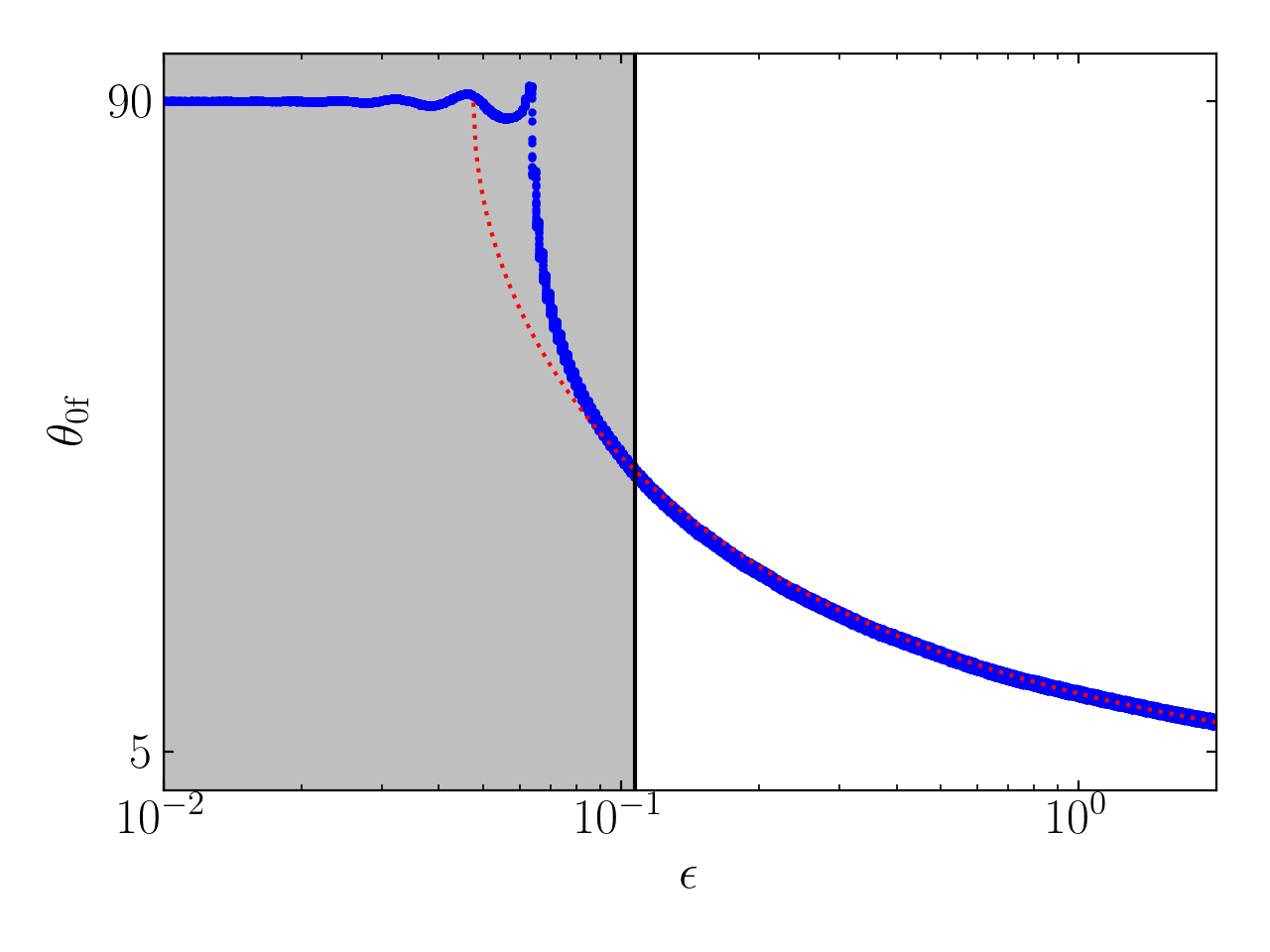
Figure 14: Final obliquity $\theta_{\rm f}$ as a function of $\epsilon$ for $\theta_{\rm sd,i}=0$ and $I=5^{\circ}$. The shaded area, bordered by the black line, corresponds to the adiabatic regime estimated by Eq. (21). The blue dots are numerical results, and the red dashed line corresponds to Eq. (40), which is in good agreement with numerical results for $\epsilon>\epsilon_{\rm c}\approx 0.1$ (the nonadiabatic regime). Note that $\theta_{\rm f}\simeq 90^{\circ}$ in the adiabatic regime ($\epsilon\ll\epsilon_{\rm c}$).

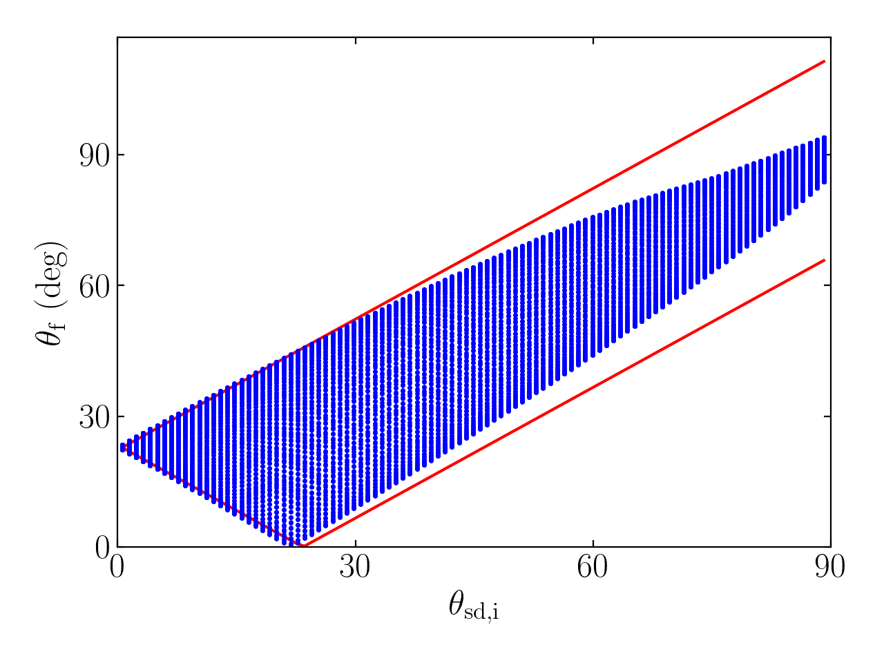
Figure 15: Final obliquity $\theta_{\rm f}$ vs $\theta_{\rm sd,i}$ for $I=5^{\circ}$ and $\epsilon=0.3$ (firmly in the nonadiabatic regime). The blue dots represent numerical results, and the two red lines show the analytical lower and upper bounds given by Eq. (41).

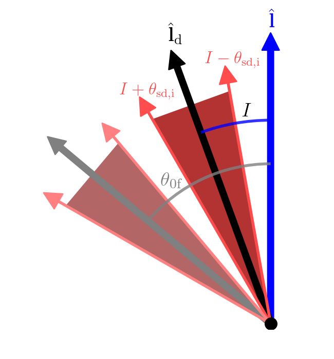
Figure 16: Schematic picture for understanding nonadiabatic obliquity evolution when $\theta_{\rm sd,i}>0$ assuming $\eta_{\rm i}\gg 1$. The figure shows a projection onto the plane containing both $\hat{\boldsymbol{\mathbf{l}}}$ and $\hat{\boldsymbol{\mathbf{l}}}_{\rm d}$. When $\theta_{\rm sd,i}=0$, the initial spin vector points along $\hat{\boldsymbol{\mathbf{l}}}_{\rm d}$ and evolves into the final spin vector (grey), which has obliquity $\theta_{\rm 0f}$ [Eq. (40)]. When $\theta_{\rm sd,i}\neq 0$, the set of initial conditions for the spin vector forms a cone (solid red area) centered on $\hat{\boldsymbol{\mathbf{l}}}_{\rm d}$ with opening half-angle $\theta_{\rm sd,i}$. Under nonadiabatic evolution, the set of final spin vectors forms a new cone, still with opening half-angle $\theta_{\rm sd,i}$, centered on $\theta_{\rm 0f}$ (light red area).

5 Summary

In this paper, we have studied the excitation of planetary obliquities due to gravitational interaction with an exterior, dissipating (mass-losing) protoplanetary disk. Obliquity excitation occurs as the system passes through a secular resonance between spin precession and orbital (nodal) precession. This scenario was recently studied by Millholland & Batygin (2019), who focused on the special case of small initial obliquities. In contrast, we consider arbitrary initial misalignment angles in this paper, motivated by the fact that planet formation through core accretion can lead to a wide range of initial spin orientations. We present our result as a mapping from $\theta_{\rm sd,i}$ to $\theta_{\rm f}$, where $\theta_{\rm sd,i}$ is the initial misalignment angle between the planet’s spin axis and the disk’s orbital angular momentum axis, and $\theta_{\rm f}$ is the final planetary obliquity. We have derived analytical results that capture the behavior of this mapping in both the adiabatic and nonadiabatic limits:

1. In the adiabatic limit (i.e. the disk dissipates at a sufficiently slow rate), we reproduce the known result $\theta_{\rm f}\simeq 90^{\circ}$ for $\theta_{\rm sd,i}\simeq 0$. We demonstrate (via numerical calculation and analytical argument) the dual-valued behavior of $\theta_{\rm f}$ for nonzero $\theta_{\rm sd,i}$ (see Fig. 5). We show for the first time that both the final $\theta_{\rm f}$ values and the probabilities of achieving each value can be understood analytically via careful accounting of adiabatic invariance and separatrix crossing dynamics.

2. As the disk dissipates more rapidly, the adiabatic condition [Eq. (21)] breaks down, we find that a broad range of final obliquities can be reached for a given $\theta_{\rm sd,i}$ (see Fig. 15). We understand this result via the novel concept of partial adiabatic resonance advection and provide an analytical expression of the bounds on $\theta_{\rm f}$ in Eq. (41).

As noted in Section 1, while in this paper we have examined a specific scenario of generating/modifying planetary obliquities from planet-disk interactions, the dynamical problem have studied is more general (Colombo, 1966; Peale, 1969, 1974; Ward, 1975; Henrard & Murigande, 1987). Our work goes beyond these previous works and provides the most general solution to the evolution of “Colombo’s top” as the system evolves from the “weak spin-orbit coupling” regime ($\eta\gg 1$) to the “strong spin-orbit coupling” regime ($\eta\ll 1$). The new analytical results presented in this paper can be adapted to other applications.

Concerning the production of planetary obliquity with a dissipating disk, when there are multiple planets in a system, the nodal precession rate $g$ for the planet of interest never decays below the Laplace-Lagrange rate driven by planet-planet secular interactions (Millholland & Batygin, 2019). Therefore, $\eta$ has a minimum value at late times. This does not affect the methodology of our analysis, but can affect the detailed results. For example, the adiabaticity criterion must be modified slightly as $\mathrm{d}\ln\eta/\mathrm{d}t$ is no longer constant but asymptotes to zero as $\eta$ decreases; the planet may never undergo separatrix crossing if their $\eta_{\star}$ (which depends on $\theta_{\rm sd,i}$) in the absence of the companions is too small; the planetary obliquity will oscillate even when the disk has fully evaporated (as $\hat{\boldsymbol{\mathbf{l}}}$ is no longer constant). The spin dynamics can be even more complex if the two planets are in mean motion resonance (e.g. Millholland & Laughlin, 2019).

Appendix A Cassini State Local Dynamics

In this appendix, we linearize the equations of motion near each CS and determine its stability. We derive the local libration frequency or growth rate for perturbations around each CS.

A.1 Canonical Equations of Motion and Solutions

We adopt spherical coordinate system where $\hat{\boldsymbol{\mathbf{l}}}=\hat{\boldsymbol{\mathbf{z}}}$ and $\theta,\phi$ are the polar and azimuthal angle of $\hat{\boldsymbol{\mathbf{s}}}$. We choose $\hat{\boldsymbol{\mathbf{l}}}_{\rm d}$ at coordinates $\theta=I,\phi=\pi$ (see Figs. 1 and 2). We use the convention $\theta\in[0,\pi)$ and $\phi\in[0,2\pi)$.

The equations of motion in $\left(\phi,\cos\theta\right)$ follow by applying Hamilton’s equations to the Hamiltonian [Eq. (15)]:

$$\frac{\mathrm{d}\phi}{\mathrm{d}t}=\frac{\partial\mathcal{H}}{\partial(\cos\theta)} =-\cos\theta+\eta\left(\cos I+\sin I\cot\theta\cos\phi\right),$$ (A1a)

$$\frac{\mathrm{d}(\cos\theta)}{\mathrm{d}t}=-\frac{\partial\mathcal{H}}{\partial\phi} =-\eta\sin I\sin\theta\sin\phi.$$ (A1b)

These agree with Eq. (9).

The CSs satisfy $\dot{\phi}=\dot{\theta}=0$. For convenience, we give approximate solutions for the CSs in the limits $\eta\ll 1$ and $\eta\gg 1$. For $\eta\ll 1$:

• CS1: $\phi_{1}=0$, $\theta_{1}\simeq\eta\sin I$.

• CS2: $\phi_{2}=\pi$, $\theta_{2}\simeq\pi/2-\eta\cos I$.

• CS3: $\phi_{3}=0$, $\theta_{3}\simeq\pi-\eta\sin I$.

• CS4: $\phi_{4}=0$, $\theta_{4}\simeq\pi/2-\eta\cos I$.

For $\eta\gg 1$, only CS2 and CS3 exist and are given by:

• CS2: $\phi_{2}=\pi$, $\theta_{2}\simeq I+\eta^{-1}\sin I\cos I$.

• CS3: $\phi_{3}=0$, $\theta_{3}\simeq\pi-I+\eta^{-1}\sin I\cos I$.

Note that in the convention of Fig. 2, CS1, CS3 and CS4 have negative $\theta$ values since $\phi=0$.

A.2 Stability and Frequency of Local Oscillations

To examine stability of each CS, we linearize Eqs. (A1) about an equilibrium located at $\phi_{\rm cs}=0$ (CS 1, 3, 4) or $\pi$ (CS2) but arbitrary $\theta_{\rm cs}$. Setting $\phi=\phi_{\rm cs}+\delta\phi,\theta=\theta_{\rm cs}+\delta\theta$ yields

$$\frac{\mathrm{d}\delta\phi}{\mathrm{d}t} =\sin\theta_{\rm cs}\delta\theta\mp\eta\frac{\sin I}{\sin^{2}\theta_{\rm cs}}\delta\theta,$$ (A2a)

$$\frac{\mathrm{d}\delta\theta}{\mathrm{d}t} =\pm\eta\sin I\delta\phi,$$ (A2b)

where the upper sign corresponds to $\phi_{\rm cs}=0$. Eliminating $\delta\theta$ gives

$$\frac{\mathrm{d}^{2}\delta\phi}{\mathrm{d}t^{2}}\equiv\lambda^{2}\delta\phi,$$ (A3)

where

$$\lambda^{2}\equiv\left(\sin\theta_{\rm cs}\mp\eta\sin I\csc^{2}\theta\right)\left(\pm\eta\sin I\right).$$ (A4)

A plot of $\lambda^{2}$ for each of the CSs is given in Fig. 17. It is clear that CS4 is unstable while the other three are stable. The local libration frequency for these stable CSs is simply $\omega_{\rm lib}=\sqrt{-\lambda^{2}}$.

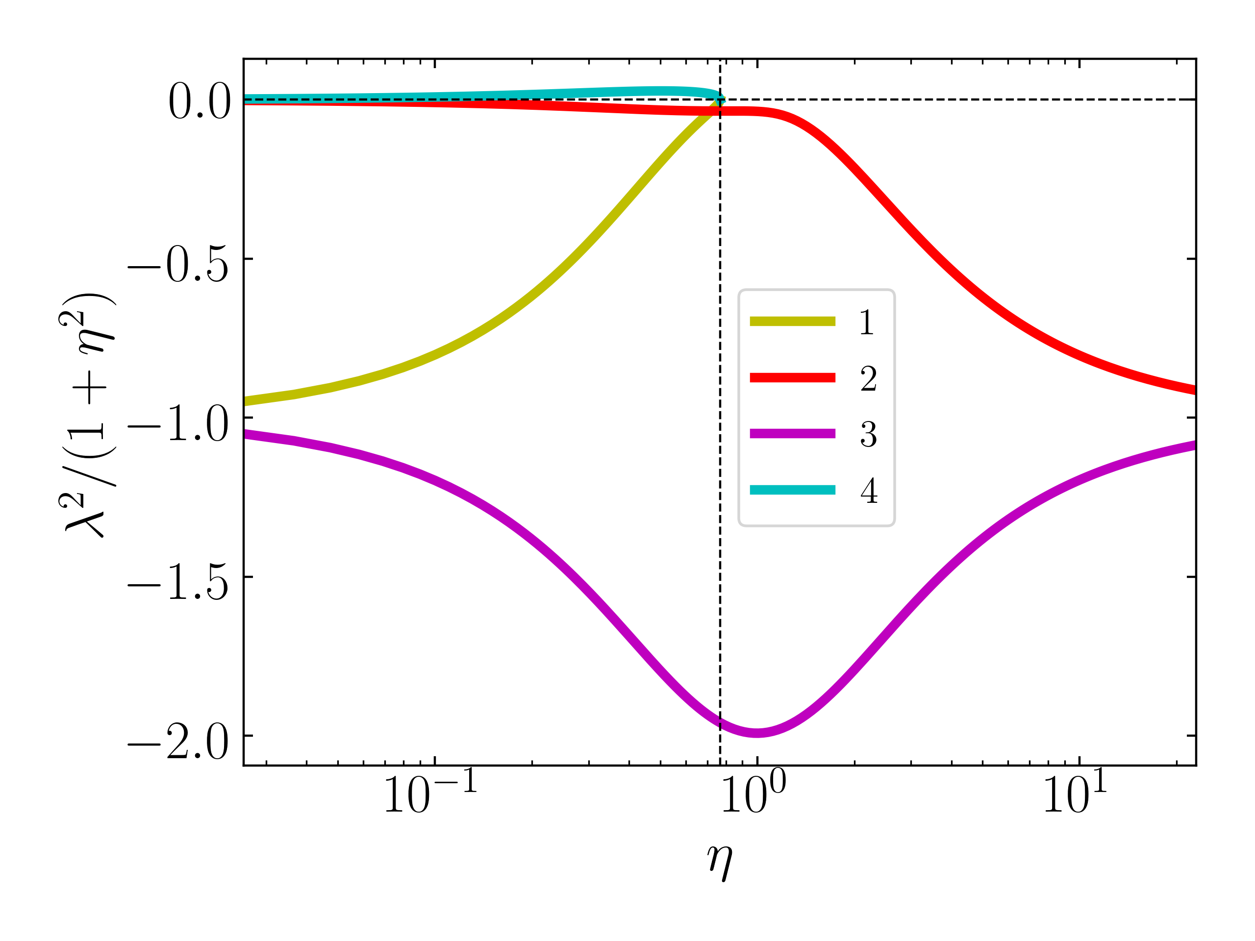
Figure 17: $\lambda^{2}$, given by Eq. (A3), evaluated at each of the Cassini States. The vertical axis is rescaled for clarity. Note that CS4 is unstable ($\lambda^{2}>0$) when it exists while all others are stable ($\lambda^{2}<0$). The thin horizontal dashed line is the instability boundary $\lambda^{2}=0$ while the thin vertical dashed line labels $\eta=\eta_{\rm c}$ [Eq. (14)].

Appendix B Approximate Adiabatic Evolution

In this appendix, we will use approximations valid for small $\eta$ to derive the explicit analytic expressions for the final obliquities at small $\theta_{\rm sd,i}$ and the associated probabilities for the II $\to$ I and II $\to$ III tracks. These are the only possible tracks for small $\eta$.

We first seek a simple parameterization for the separatrix, the level curve of the Hamiltonian intersecting the unstable equilibrium CS4. Points along the separatrix, parameterized by $\left(\phi,\theta_{\rm sep}(\phi)\right)$, satisfy $\mathcal{H}\left(\phi,\theta_{\rm sep}(\phi)\right)=\mathcal{H}\left(\phi_{4},\theta_{4}\right)$ where $\phi_{4}$ and $\theta_{4}$ are given in Appendix A.1. We obtain two solutions for $\theta_{\rm sep}$, given to leading order in $\eta$ by:

$$\cos\theta_{\rm sep}(\phi)\approx\cos\theta_{4}\pm\sqrt{2\eta\sin I\left(1-\cos\phi\right)}.$$ (B1)

These two solutions parameterize the two legs of the separatrix. Integration of the phase area enclosed by the separatrix yields then

$$\mathcal{A}_{\rm II}(\eta)\approx 16\sqrt{\eta\sin I}.$$ (B2)

We can now compute the final obliquities and their associated probabilities for each track as follows:

1. For a given $\theta_{\rm sd,i}$, we know that if $\eta\to\infty$ then the trajectory executes simple libration about $\hat{\boldsymbol{\mathbf{l}}}_{\rm d}$, and so $A=2\pi\left(1-\cos\theta_{\rm sd,i}\right)\approx\pi\theta_{\rm sd,i}^{2}$. This then implies $\eta_{\star}$ must be the solution to $\mathcal{A}_{\rm II}(\eta_{\star})=A$, or

   $$\eta_{\star}\approx\left(\frac{2\pi\left(1-\cos\theta_{\rm sd,i}\right)}{16}\right)^{2}\frac{1}{\sin I}\approx\left(\frac{\pi\theta_{\rm sd,i}^{2}}{16}\right)^{2}\frac{1}{\sin I}.$$ (B3)

2. Upon separatrix encounter, a transition to either zone I or zone III occurs. These can be calculated to have the associated probabilities [using the approximate area Eq. (B2) and Eqs. (25)]

   $$\Pr\left(\rm II\to I\right) \approx\frac{2\pi\eta_{\star}\cos I+4\sqrt{\eta_{\star}\sin I}}{8\sqrt{\eta_{\star}\sin I}},$$ (B4a)

   $$\Pr\left(\rm II\to III\right) \approx\frac{-2\pi\eta_{\star}\cos I+4\sqrt{\eta_{\star}\sin I}}{8\sqrt{\eta_{\star}\sin I}}.$$ (B4b)

3. Upon a transition to zone I or zone III, the final obliquity can be predicted by observing the final adiabatic invariant $A_{\rm f}=-\mathcal{A}_{\rm I}(\eta_{\star})$ in the zone I case and $A_{\rm f}=\mathcal{A}_{\rm I}(\eta_{\star})+\mathcal{A}_{\rm I}I(\eta_{\star})$ in the zone III case. As $\eta\to 0$, these correspond to obliquities

   $$\left(\cos\theta_{\rm f}\right)_{\rm II\to I} \approx\left(\frac{\pi\theta_{\rm sd,i}^{2}}{16}\right)^{2}\cot I+\frac{\theta_{\rm sd,i}^{2}}{4},$$ (B5a)

   $$\left(\cos\theta_{\rm f}\right)_{\rm II\to III} \approx\left(\frac{\pi\theta_{\rm sd,i}^{2}}{16}\right)^{2}\cot I-\frac{\theta_{\rm sd,i}^{2}}{4}.$$ (B5b)

   These are the black dotted lines overplotted in Fig. 5.

References

- Adams et al. (2019) Adams, A. D., Millholland, S., & Laughlin, G. P. 2019, arXiv preprint arXiv:1906.07615
- Anderson & Lai (2018) Anderson, K. R., & Lai, D. 2018, Monthly Notices of the Royal Astronomical Society, 480, 1402
- Batygin & Adams (2013) Batygin, K., & Adams, F. C. 2013, The Astrophysical Journal, 778, 169
- Benz et al. (1989) Benz, W., Slattery, W., & Cameron, A. 1989, Meteoritics, 24, 251
- Bryan et al. (2018) Bryan, M. L., Benneke, B., Knutson, H. A., Batygin, K., & Bowler, B. P. 2018, Nature Astronomy, 2, 138
- Bryan et al. (2020) Bryan, M. L., Chiang, E., Bowler, B. P., et al. 2020, The Astronomical Journal, 159, 181
- Colombo (1966) Colombo, G. 1966, SAO Special Report, 203
- Correia et al. (2003) Correia, A. C., Laskar, J., & de Surgy, O. N. 2003, Icarus, 163, 1
- Dones & Tremaine (1993) Dones, L., & Tremaine, S. 1993, Science, 259, 350
- Fabrycky et al. (2007) Fabrycky, D. C., Johnson, E. T., & Goodman, J. 2007, The Astrophysical Journal, 665, 754
- Hamilton & Ward (2004) Hamilton, D. P., & Ward, W. R. 2004, The Astronomical Journal, 128, 2510
- Henrard (1982) Henrard, J. 1982, Celestial Mechanics and Dynamical Astronomy, 27, 3
- Henrard & Murigande (1987) Henrard, J., & Murigande, C. 1987, Celestial Mechanics, 40, 345
- Inamdar & Schlichting (2015) Inamdar, N. K., & Schlichting, H. E. 2015, Monthly Notices of the Royal Astronomical Society, 448, 1751
- Izidoro et al. (2017) Izidoro, A., Ogihara, M., Raymond, S. N., et al. 2017, Monthly Notices of the Royal Astronomical Society, 470, 1750
- Korycansky et al. (1990) Korycansky, D., Bodenheimer, P., Cassen, P., & Pollack, J. 1990, Icarus, 84, 528
- Lai (2014) Lai, D. 2014, Monthly Notices of the Royal Astronomical Society, 440, 3532
- Lainey (2016) Lainey, V. 2016, Celestial Mechanics and Dynamical Astronomy, 126, 145
- Laskar & Robutel (1993) Laskar, J., & Robutel, P. 1993, Nature, 361, 608
- Lissauer et al. (1997) Lissauer, J. J., Berman, A. F., Greenzweig, Y., & Kary, D. M. 1997, Icarus, 127, 65
- Miguel & Brunini (2010) Miguel, Y., & Brunini, A. 2010, Monthly Notices of the Royal Astronomical Society, 406, 1935
- Millholland & Batygin (2019) Millholland, S., & Batygin, K. 2019, The Astrophysical Journal, 876, 119
- Millholland & Laughlin (2018) Millholland, S., & Laughlin, G. 2018, The Astrophysical Journal Letters, 869, L15
- Millholland & Laughlin (2019) —. 2019, Nature Astronomy, 3, 424
- Morbidelli et al. (2012) Morbidelli, A., Tsiganis, K., Batygin, K., Crida, A., & Gomes, R. 2012, Icarus, 219, 737
- Ohno & Zhang (2019) Ohno, K., & Zhang, X. 2019, The Astrophysical Journal, 874, 2
- Peale (1969) Peale, S. J. 1969, The Astronomical Journal, 74, 483
- Peale (1974) —. 1974, The Astronomical Journal, 79, 722
- Rogoszinski & Hamilton (2019) Rogoszinski, Z., & Hamilton, D. P. 2019, arXiv preprint arXiv:1908.10969
- Safronov & Zvjagina (1969) Safronov, V., & Zvjagina, E. 1969, Icarus, 10, 109
- Seager & Hui (2002) Seager, S., & Hui, L. 2002, The Astrophysical Journal, 574, 1004
- Snellen et al. (2014) Snellen, I. A., Brandl, B. R., de Kok, R. J., et al. 2014, Nature, 509, 63
- Touma & Wisdom (1993) Touma, J., & Wisdom, J. 1993, Science, 259, 1294
- Vokrouhlickỳ & Nesvornỳ (2015) Vokrouhlickỳ, D., & Nesvornỳ, D. 2015, The Astrophysical Journal, 806, 143
- Ward (1975) Ward, W. R. 1975, The Astronomical Journal, 80, 64
- Ward & Hamilton (2004) Ward, W. R., & Hamilton, D. P. 2004, The Astronomical Journal, 128, 2501
- Zanazzi & Lai (2018) Zanazzi, J., & Lai, D. 2018, Monthly Notices of the Royal Astronomical Society, 478, 835