11institutetext: R. Madani 22institutetext: M. Kheirandishfard33institutetext: 517 Nedderman Hall, University of Texas, Arlington, TX 76019, USA
33email: ramtin.madani@uta.edu,mohsen.kheirandishfard@mavs.uta.edu
44institutetext: J. Lavaei and A. Atamtürk 55institutetext: 4175 Etcheverry Hall, University of California, Berkeley, CA 94720, USA
Tel.: +1-510-642-4559
55email: lavaei@berkeley.edu,atamturk@berkeley.edu

Penalized Semidefinite Programming for Quadratically-Constrained Quadratic Optimization thanks: This work is in part supported by the NSF Award 1809454. Javad Lavaei is supported by an AFOSR YIP Award and ONR N000141712933. Alper Atamtürk is supported, in part, by grant FA9550-10-1-0168 from the Office of the Assistant Secretary of Defense for Research & Engineering, NSF award 1807260, DOE ARPA-E award 260801540061, and ONR award 12951270.

Ramtin Madani    Mohsen Kheirandishfard    Javad Lavaei    Alper Atamtürk
(Received: date / Accepted: date)
Abstract

In this paper, we give a new penalized semidefinite programming approach for non-convex quadratically-constrained quadratic programs (QCQPs). We incorporate penalty terms into the objective of convex relaxations in order to retrieve feasible and near-optimal solutions for non-convex QCQPs. We introduce a generalized linear independence constraint qualification (GLICQ) criterion and prove that any GLICQ regular point that is sufficiently close to the feasible set can be used to construct an appropriate penalty term and recover a feasible solution. Inspired by these results, we develop a heuristic sequential procedure that preserves feasibility and aims to improve the objective value at each iteration. Numerical experiments on large-scale system identification problems as well as benchmark instances from the library of quadratic programming (QPLIB) demonstrate the ability of the proposed penalized semidefinite programs in finding near-optimal solutions for non-convex QCQP.

Keywords:
Semidefinite programming non-convex optimization non-linear programming convex relaxation
pacs:
87.55.de
MSC:
65K05 90-08 90C26 90C22

1 Introduction

This paper studies a subclass of polynomial optimization, referred to as quadratically-constrained quadratic programming (QCQP), which minimizes a quadratic function within a feasible set that is also characterized by quadratic functions. QCQP arises in various scientific and engineering applications, such as electric power systems Madani et al. (2016, 2015b, 2015a, 2017b), imaging science Bandeira et al. (2014); Candes et al. (2015); Fogel et al. (2016); Singer (2011), signal processing Aittomaki and Koivunen (2009); Aubry et al. (2013); Chen and Vaidyanathan (2009); Li et al. (2012); Luo et al. (2010); Mariere et al. (2003), automatic control Fazelnia et al. (2017); Toker and Ozbay (1998); Madani et al. (2017b); Ahmadi and Majumdar (2019), quantum mechanics Hilling and Sudbery (2010); Deza and Laurent (1994); Laurent and Piovesan (2015); Burgdorf et al. (2015), and cybersecurity Cid et al. (2005, 2004); Courtois and Pieprzyk (2002); Murphy and Robshaw (2002). The development of efficient optimization techniques and numerical algorithms for QCQP has been an active area of research for decades. Due to the barriers imposed by NP-hardness, the focus of some research efforts has shifted from designing general-purpose algorithms to specialized methods that are robust and scalable for specific application domains. Notable examples for which methods with guaranteed performance have been offered in the literature include the problems of multisensor beamforming in communication theory Gershman et al. (2010), phase retrieval in signal processing Candes et al. (2013), and matrix completion in machine learning Mu et al. (2016); Candès and Recht (2009).

This paper advances a popular framework for the global analysis of QCQP through semidefinite programming (SDP) relaxations Sherali and Adams (1990); Nesterov et al. (1994); Lasserre (2001b, 2006); Josz and Molzahn (2018); Chen and Burer (2012); Papp and Alizadeh (2013); Mohammad-Nezhad and Terlaky (2017). A relaxation is said to be exact if it has the same optimal objective value as the original problem. SDP has been critically important for constructing strong convex relaxations of non-convex optimization problems and its exactness has been verified for numerous real-world problems Lasserre (2001a); Kim and Kojima (2003); Sojoudi and Lavaei (2013a, b); Burer and Ye (2018). Additionally, for many problems where an exact relaxation is not available, SDP relaxations have offered effective approximation algorithms Nesterov (1998); Ye (1999b, a); Zhang (2000); Zhang and Huang (2006); Luo et al. (2007); He et al. (2008, 2010). Geomans and Williamson Goemans and Williamson (1995) show that an SDP relaxation objective is within 14% of the optimal value for the MAXCUT problem on graphs with non-negative weights. Additionally, SDP relaxations are used within branch-and-bound algorithms Chen et al. (2017); Burer and Vandenbussche (2008) for finding globally optimal solutions to non-convex optimization problems.

In particular, forming hierarchies of SDP relaxations Lovász and Schrijver (1991); Sherali and Adams (1990); Lasserre (2001b, 2006); Josz and Molzahn (2018); Chen and Burer (2012); Papp and Alizadeh (2013); Mohammad-Nezhad and Terlaky (2017) has been proven to yield the convex hull of non-convex QCQP problems. Despite solid theoretical guarantees, one of the primary challenges for the application of SDP hierarchies beyond small-scale instances is the rapid growth of dimensionality. In response, one direction of research has exploited sparsity and structural patterns to boost efficiency Atamtürk and Gómez (2019); Han et al. (2020); Muramatsu and Suzuki (2003); Kim et al. (2003); Kim and Kojima (2003); Bao et al. (2011); Natarajan et al. (2013). Another direction, pursued in Alizadeh and Goldfarb (2003); Atamtürk and Narayanan (2007); Majumdar et al. (2014); Permenter and Parrilo (2018); Madani et al. (2017a); Ahmadi and Majumdar (2019); Bienstock and Munoz (2018), is to use lower-complexity relaxations as alternatives to computationally demanding SDP relaxations. In this paper, we offer an alternative approach, which focuses on penalizing the objective function of the SDP relaxations as opposed to strengthening the quality of the relaxations, which can be computationally prohibitive. We show that under certain conditions, incorporating a penalty term in the objective can remedy inexact relaxations and lead to feasible points for non-convex QCQPs.

1.1 Contributions

This paper is concerned with non-convex quadratically-constrained quadratic programs for which SDP relaxations are inexact. In order to recover feasible points for QCQP, we incorporate a linear penalty term into the objective of SDP relaxations and show that feasible and near-globally optimal points can be obtained for the original QCQP by solving the resulting penalized SDPs. The penalty term is based on an arbitrary initial point. Our first result states that if the initial point is feasible and satisfies the linear independence constraint qualification (LICQ) condition, then penalized SDP produces a unique solution that is feasible for the original QCQP and its objective value is not worse than that of the initial point. Our second result states that if the initial point is infeasible, but instead is sufficiently close to the feasible set and satisfies a generalized LICQ condition, then the unique optimal solution to penalized SDP is feasible for QCQP. Lastly, motivated by these results on constructing feasible points, we propose a heuristic sequential procedure for non-convex QCQP and demonstrate its performance on benchmark instances from the QPLIB library Furini et al. (2019) as well as on large-scale system identification problems.

The success of sequential frameworks and penalized SDP in solving bilinear matrix inequalities (BMIs) is demonstrated in Ibaraki and Tomizuka (2001); Kheirandishfard et al. (2018c, a). In Ashraphijuo et al. (2016), it is shown that penalized SDP is able to find the roots of overdetermined systems of polynomial equations. Moreover, the incorporation of penalty terms into the objective of SDP relaxations are proven to be effective for solving non-convex optimization problems in power systems Madani et al. (2015b, 2016); Zohrizadeh et al. (2018b, a). These papers show that penalizing certain physical quantities in power network optimization problems such as reactive power loss or thermal loss facilitates the recovery of feasible points from convex relaxations. In Ibaraki and Tomizuka (2001), a sequential framework is introduced for solving BMIs without theoretical guarantees. Papers Kheirandishfard et al. (2018c, a) investigate this approach further and offer theoretical results through the notion of generalized Mangasarian-Fromovitz regularity condition. However, these conditions are not valid in the presence of equality constraints and for general QCQPs. Motivated by the success of penalized SDP, this paper offers a theoretical framework for general QCQP and, by extension, polynomial optimization problems.

1.2 Notations

Throughout the paper, scalars, vectors, and matrices are respectively shown by italic letters, lower-case italic bold letters, and upper-case italic bold letters. The symbols \mathbb{R}, nsuperscript𝑛\mathbb{R}^{n}, and n×msuperscript𝑛𝑚\mathbb{R}^{n\times m} denote the sets of real scalars, real vectors of size n𝑛n, and real matrices of size n×m𝑛𝑚n\times m, respectively. The set of n×n𝑛𝑛n\times n real symmetric matrices is shown by 𝕊nsubscript𝕊𝑛\mathbb{S}_{n}. For a given vector 𝒂𝒂\boldsymbol{a} and a matrix 𝑨𝑨\boldsymbol{A}, the symbols aisubscript𝑎𝑖a_{i} and Aijsubscript𝐴𝑖𝑗A_{ij} respectively indicate the ithsuperscript𝑖𝑡i^{th} element of 𝒂𝒂\boldsymbol{a} and the (i,j)thsuperscript𝑖𝑗th(i,j)^{\mathrm{th}} element of 𝑨𝑨\boldsymbol{A}. The symbols ,\langle\cdot\,,\cdot\rangle and F\|\cdot\|_{\mathrm{F}} denote the Frobenius inner product and norm of matrices, respectively. The notation |||\cdot| represents either the absolute value operator or cardinality of a set, depending on the context. The notation 2\|\cdot\|_{2} denotes the 2subscript2\ell_{2} norm of vectors, matrices, and matrix pencils. The n×n𝑛𝑛n\times n identity matrix is denoted by 𝑰nsubscript𝑰𝑛\boldsymbol{I}_{n}. The origin of nsuperscript𝑛\mathbb{R}^{n} is denoted by 𝟎nsubscript0𝑛\boldsymbol{0}_{n}. The superscript ()superscripttop(\cdot)^{\top} and the symbol tr{}tr\mathrm{tr}\{\cdot\} represent the transpose and trace operators, respectively. Given a matrix 𝑨m×n𝑨superscript𝑚𝑛\boldsymbol{A}\in\mathbb{R}^{m\times n}, the notation σmin(𝑨)subscript𝜎𝑨\sigma_{\min}(\boldsymbol{A}) represents the minimum singular value of 𝑨𝑨\boldsymbol{A}. The notation 𝑨0succeeds-or-equals𝑨0\boldsymbol{A}\succeq 0 means that 𝑨𝑨\boldsymbol{A} is symmetric positive-semidefinite. For a pair of n×n𝑛𝑛n\times n symmetric matrices (𝑨,𝑩)𝑨𝑩(\boldsymbol{A},\boldsymbol{B}) and proper cone 𝒞𝕊n𝒞subscript𝕊𝑛\mathcal{C}\subseteq\mathbb{S}_{n}, the notation 𝑨𝒞𝑩subscriptsucceeds-or-equals𝒞𝑨𝑩\boldsymbol{A}\succeq_{\mathcal{C}}\boldsymbol{B} means that 𝑨𝑩𝒞𝑨𝑩𝒞\boldsymbol{A}-\boldsymbol{B}\in\mathcal{C}, whereas 𝑨𝒞𝑩subscriptsucceeds𝒞𝑨𝑩\boldsymbol{A}\succ_{\mathcal{C}}\boldsymbol{B} means that 𝑨𝑩𝑨𝑩\boldsymbol{A}-\boldsymbol{B} belongs to the interior of 𝒞𝒞\mathcal{C}. Given an integer r>1𝑟1r>1, define 𝒞rsubscript𝒞𝑟\mathcal{C}_{r} as the cone of n×n𝑛𝑛n\times n symmetric matrices whose r×r𝑟𝑟r\times r principal submatrices are all positive semidefinite. Similarly, define 𝒞rsubscriptsuperscript𝒞𝑟\mathcal{C}^{\ast}_{r} as the dual cone of 𝒞rsubscript𝒞𝑟\mathcal{C}_{r}, i.e., the cone of n×n𝑛𝑛n\times n symmetric matrices whose every r×r𝑟𝑟r\times r principal submatrix is positive semidefinite (i.e., factor-width bounded by r𝑟r). Given a matrix 𝑨m×n𝑨superscript𝑚𝑛\boldsymbol{A}\in\mathbb{R}^{m\times n} and two sets of positive integers 𝒮1subscript𝒮1\mathcal{S}_{1} and 𝒮2subscript𝒮2\mathcal{S}_{2}, define 𝑨{𝒮1,𝒮2}𝑨subscript𝒮1subscript𝒮2\boldsymbol{A}\{\mathcal{S}_{1},\mathcal{S}_{2}\} as the submatrix of 𝑨𝑨\boldsymbol{A} obtained by removing all rows of 𝑨𝑨\boldsymbol{A} whose indices do not belong to 𝒮1subscript𝒮1\mathcal{S}_{1}, and all columns of 𝑨𝑨\boldsymbol{A} whose indices do not belong to 𝒮2subscript𝒮2\mathcal{S}_{2}. Moreover, define 𝑨{𝒮1}𝑨subscript𝒮1\boldsymbol{A}\{\mathcal{S}_{1}\} as the submatrix of 𝑨𝑨\boldsymbol{A} obtained by removing all rows of 𝑨𝑨\boldsymbol{A} that do not belong to 𝒮1subscript𝒮1\mathcal{S}_{1}. Given a vector 𝒂n𝒂superscript𝑛\boldsymbol{a}\in\mathbb{R}^{n} and a set nsuperscript𝑛\mathcal{F}\subseteq\mathbb{R}^{n}, define d(𝒂)subscript𝑑𝒂d_{\mathcal{F}}(\boldsymbol{a}) as the minimum distance between 𝒂𝒂\boldsymbol{a} and members of \mathcal{F}. Given a pair of integers (n,r)𝑛𝑟(n,r), the binomial coefficient “n𝑛n choose r𝑟r” is denoted by (nr)binomial𝑛𝑟n\choose r. The notations 𝒙f(𝒂)subscript𝒙𝑓𝒂\nabla_{\boldsymbol{x}}f(\boldsymbol{a}) and 𝒙2f(𝒂)subscriptsuperscript2𝒙𝑓𝒂\nabla^{2}_{\boldsymbol{x}}f(\boldsymbol{a}), respectively, represent the gradient and Hessian of the function f𝑓f, with respect to the vector 𝒙𝒙\boldsymbol{x}, at a point 𝒂𝒂\boldsymbol{a}.

1.3 Outline

The remainder of the paper is organized as follows. In Section 2, we review the basic lifted and reformulation linearization technique (RLT) as well as the standard SDP relaxations. Section 3 presents the main results of the paper: the penalized SDP, its theoretical analysis on producing a feasible solution along with a generalized linear independence constraint qualification, and finally the sequential penalization procedure. In Section 4 we present numerical experiments to test the effectiveness of the sequential penalization approach for non-convex QCQPs from the library of quadratic programming instances (QPLIB) as well as large-scale system identification problems. Finally, we conclude in section 5 with a few final remarks.

2 Preliminaries

In this section, we review the lifting and reformulation-linearization technique (RLT) as well as the standard convex relaxations of QCQP that are necessary for the development of the main results on penalized SDP in Section 3. Consider a general quadratically-constrained quadratic program (QCQP):

minimize𝒙n𝒙superscript𝑛minimize\displaystyle\underset{\boldsymbol{x}\in\mathbb{R}^{n}}{\text{minimize}}\ \ q0(𝒙)subscript𝑞0𝒙\displaystyle q_{0}(\boldsymbol{x}) (1a)
s.t. qk(𝒙)0,kformulae-sequencesubscript𝑞𝑘𝒙0𝑘\displaystyle q_{k}(\boldsymbol{x})\leq 0,\ \ k\in\mathcal{I} (1b)
qk(𝒙)=0,k,formulae-sequencesubscript𝑞𝑘𝒙0𝑘\displaystyle q_{k}(\boldsymbol{x})=0,\ \ k\in\mathcal{E}, (1c)

where \mathcal{I} and \mathcal{E} index the sets of inequality and equality constraints, respectively. For every k{0}𝑘0k\in\{0\}\cup\mathcal{I}\cup\mathcal{E}, qk:n:subscript𝑞𝑘superscript𝑛q_{k}:\mathbb{R}^{n}\to\mathbb{R} is a quadratic function of the form qk(𝒙)𝒙𝑨k𝒙+2𝒃k𝒙+cksubscript𝑞𝑘𝒙superscript𝒙topsubscript𝑨𝑘𝒙2subscriptsuperscript𝒃top𝑘𝒙subscript𝑐𝑘q_{k}(\boldsymbol{x})\triangleq\boldsymbol{x}^{\top}\boldsymbol{A}_{k}\boldsymbol{x}+2\boldsymbol{b}^{\top}_{k}\boldsymbol{x}+c_{k}, where 𝑨k𝕊nsubscript𝑨𝑘subscript𝕊𝑛\boldsymbol{A}_{k}\in\mathbb{S}_{n}, 𝒃knsubscript𝒃𝑘superscript𝑛\boldsymbol{b}_{k}\in\mathbb{R}^{n}, and cksubscript𝑐𝑘c_{k}\in\mathbb{R}. Denote \mathcal{F} as the feasible set of the QCQP (1a)–(1c). To derive the optimality conditions for a given point, it is useful to define the Jacobian matrix of the constraint functions.

Definition 1 (Jacobian Matrix)

For every 𝒙^n^𝒙superscript𝑛\hat{\boldsymbol{x}}\in\mathbb{R}^{n}, the Jacobian matrix 𝒥(𝒙^)𝒥^𝒙\mathcal{J}(\hat{\boldsymbol{x}}) for the constraint functions {qk}ksubscriptsubscript𝑞𝑘𝑘\{q_{k}\}_{k\in\mathcal{I}\cup\mathcal{E}} is

𝒥(𝒙^)𝒥^𝒙\displaystyle\mathcal{J}(\hat{\boldsymbol{x}}) [𝒙q1(𝒙^),,𝒙q||(𝒙^)].absentsuperscriptsubscript𝒙subscript𝑞1^𝒙subscript𝒙subscript𝑞^𝒙top\displaystyle\triangleq[\nabla_{\boldsymbol{x}}q_{1}(\hat{\boldsymbol{x}}),\ldots,\nabla_{\boldsymbol{x}}q_{|\mathcal{I}\cup\mathcal{E}|}(\hat{\boldsymbol{x}})]^{\top}. (2)

For every 𝒬𝒬\mathcal{Q}\subseteq\mathcal{I}\cup\mathcal{E}, define 𝒥𝒬(𝒙^)subscript𝒥𝒬^𝒙\mathcal{J}_{\mathcal{Q}}(\hat{\boldsymbol{x}}) as the submatrix of 𝒥(𝒙^)𝒥^𝒙\mathcal{J}(\hat{\boldsymbol{x}}) resulting from the rows that belong to 𝒬𝒬\mathcal{Q}.

Given a feasible point for the QCQP (1a)–(1c), the well-known linear independence constraint qualification (LICQ) condition can be used as a regularity criterion.

Definition 2 (LICQ Condition)

A feasible point 𝒙^^𝒙\hat{\boldsymbol{x}}\in\mathcal{F} is LICQ regular if the rows of 𝒥^(𝒙^)subscript𝒥^^𝒙\mathcal{J}_{\hat{\mathcal{B}}}(\hat{\boldsymbol{x}}) are linearly independent, where ^{k|qk(𝒙^)=0}^conditional-set𝑘subscript𝑞𝑘^𝒙0\hat{\mathcal{B}}\triangleq\{k\in\mathcal{I}\cup\mathcal{E}\;|\;q_{k}(\hat{\boldsymbol{x}})=0\} denotes the set of binding constraints at 𝒙^^𝒙\hat{\boldsymbol{x}}.

Finding a feasible point for the QCQP (1a)–(1c), however, is NP-hard as the Boolean Satisfiability Problem (SAT) is a special case. Therefore, in Section 3, we introduce the notion of generalized LICQ as a regularity condition for both feasible and infeasible points.

2.1 Convex relaxation

A common approach for tackling the non-convex QCQP (1a)–(1c) introduces an auxiliary variable 𝑿𝕊n𝑿subscript𝕊𝑛\boldsymbol{X}\in\mathbb{S}_{n} accounting for 𝒙𝒙𝒙superscript𝒙top\boldsymbol{x}\boldsymbol{x}^{\top}. Then, the objective function (1a) and constraints (1b)–(1c) can be written as linear functions of 𝒙𝒙\boldsymbol{x} and 𝑿𝑿\boldsymbol{X}. For every k{0}𝑘0k\in\{0\}\cup\mathcal{I}\cup\mathcal{E}, define q¯k:n×𝕊n:subscript¯𝑞𝑘superscript𝑛subscript𝕊𝑛\bar{q}_{k}:\mathbb{R}^{n}\times\mathbb{S}_{n}\to\mathbb{R} as

q¯k(𝒙,𝑿)𝑨k,𝑿+2𝒃k𝒙+ck.subscript¯𝑞𝑘𝒙𝑿subscript𝑨𝑘𝑿2subscriptsuperscript𝒃top𝑘𝒙subscript𝑐𝑘\displaystyle\bar{q}_{k}(\boldsymbol{x},\boldsymbol{X})\triangleq\langle\boldsymbol{A}_{k},\boldsymbol{X}\rangle+2\boldsymbol{b}^{\top}_{k}\boldsymbol{x}+c_{k}. (3)

Consider the following relaxation of QCQP (1a)–(1c):

minimize𝒙n,𝑿𝕊nformulae-sequence𝒙superscript𝑛𝑿subscript𝕊𝑛minimize\displaystyle\underset{\begin{subarray}{l}\boldsymbol{x}\in\mathbb{R}^{n},\boldsymbol{X}\in\mathbb{S}_{n}\end{subarray}}{\text{minimize}}\ \ q¯0(𝒙,𝑿)subscript¯𝑞0𝒙𝑿\displaystyle\bar{q}_{0}(\boldsymbol{x},\boldsymbol{X}) (4a)
s.t. q¯k(𝒙,𝑿)0,kformulae-sequencesubscript¯𝑞𝑘𝒙𝑿0𝑘\displaystyle\bar{q}_{k}(\boldsymbol{x},\boldsymbol{X})\leq 0,\qquad\qquad k\in\mathcal{I} (4b)
q¯k(𝒙,𝑿)=0,kformulae-sequencesubscript¯𝑞𝑘𝒙𝑿0𝑘\displaystyle\bar{q}_{k}(\boldsymbol{x},\boldsymbol{X})=0,\qquad\qquad k\in\mathcal{E} (4c)
𝑿𝒙𝒙𝒞r0subscriptsucceeds-or-equalssubscript𝒞𝑟𝑿𝒙superscript𝒙top0\displaystyle\boldsymbol{X}-\boldsymbol{x}\boldsymbol{x}^{\top}\succeq_{\mathcal{C}_{r}}0 (4d)

where the additional conic constraint (4d) is a convex relaxation of the equation 𝑿=𝒙𝒙𝑿𝒙superscript𝒙top\boldsymbol{X}=\boldsymbol{x}\boldsymbol{x}^{\top}. We refer to the convex problem (4a)–(4d) as the r×r𝑟𝑟r\times r SDP relaxation of the QCQP (1a)–(1c). The choice r=n𝑟𝑛r=n yields the well-known semidefinite programming (SDP) relaxation. Additionally, in the homogeneous case (i.e., if 𝒃0=𝒃1==𝒃||=𝟎subscript𝒃0subscript𝒃1subscript𝒃0\boldsymbol{b}_{0}=\boldsymbol{b}_{1}=\dots=\boldsymbol{b}_{|\mathcal{I}\cup\mathcal{E}|}=\boldsymbol{0}), the case r=2𝑟2r=2 leads to the second-order conic programming (SOCP) relaxation.

In the presence of affine constraints, the RLT method of Sherali and Adams Sherali and Adams (2013) can be used to produce additional inequalities with respect to 𝒙𝒙\boldsymbol{x} and 𝑿𝑿\boldsymbol{X} to strengthen convex relaxations. This is covered in Appendix B.

If the relaxed problem (4a)–(4d) has an optimal solution (𝒙,𝑿)𝒙𝑿(\accentset{\ast}{\boldsymbol{x}},\accentset{\ast}{\boldsymbol{X}}) that satisfies 𝑿=𝒙𝒙𝑿𝒙superscript𝒙top\accentset{\ast}{\boldsymbol{X}}=\accentset{\ast}{\boldsymbol{x}}\accentset{\ast}{\boldsymbol{x}}^{\top}, then the relaxation is said to be exact and 𝒙𝒙\accentset{\ast}{\boldsymbol{x}} is a globally optimal solution for the QCQP (1a)–(1c). The next section offers a penalization method for addressing the case where relaxations are not exact.

3 Penalized SDP

If the relaxed problem (4a)–(4d) is not exact, the resulting solution is not necessarily feasible for the original QCQP (1a)–(1c). In this case, we use an initial point 𝒙^n^𝒙superscript𝑛\hat{\boldsymbol{x}}\in\mathbb{R}^{n} (either feasible or infeasible) to revise the objective function, resulting in a penalized SDP of the form:

minimize𝒙n,𝑿𝕊nformulae-sequence𝒙superscript𝑛𝑿subscript𝕊𝑛minimize\displaystyle\underset{\begin{subarray}{l}\boldsymbol{x}\in\mathbb{R}^{n},\boldsymbol{X}\in\mathbb{S}_{n}\end{subarray}}{\text{minimize}}\ \ q¯0(𝒙,𝑿)+η×(tr{𝑿}2𝒙^𝒙+𝒙^𝒙^)subscript¯𝑞0𝒙𝑿𝜂tr𝑿2superscript^𝒙top𝒙superscript^𝒙top^𝒙\displaystyle\bar{q}_{0}(\boldsymbol{x},\boldsymbol{X})+\eta\times(\mathrm{tr}\{\boldsymbol{X}\}-2\hat{\boldsymbol{x}}^{\!\top}\boldsymbol{x}+\hat{\boldsymbol{x}}^{\!\top}\hat{\boldsymbol{x}}) (5a)
s.t. q¯k(𝒙,𝑿)0,kformulae-sequencesubscript¯𝑞𝑘𝒙𝑿0𝑘\displaystyle\bar{q}_{k}(\boldsymbol{x},\boldsymbol{X})\leq 0,\qquad\qquad k\in\mathcal{I} (5b)
q¯k(𝒙,𝑿)=0,kformulae-sequencesubscript¯𝑞𝑘𝒙𝑿0𝑘\displaystyle\bar{q}_{k}(\boldsymbol{x},\boldsymbol{X})=0,\qquad\qquad k\in\mathcal{E} (5c)
𝑿𝒙𝒙𝒞r0subscriptsucceeds-or-equalssubscript𝒞𝑟𝑿𝒙superscript𝒙top0\displaystyle\boldsymbol{X}-\boldsymbol{x}\boldsymbol{x}^{\top}\succeq_{\mathcal{C}_{r}}0 (5d)

where η>0𝜂0\eta>0 is a fixed penalty parameter. Note that the penalty term tr{𝑿}2𝒙^𝒙+𝒙^𝒙^tr𝑿2superscript^𝒙top𝒙superscript^𝒙top^𝒙\mathrm{tr}\{\boldsymbol{X}\}-2\hat{\boldsymbol{x}}^{\!\top}\boldsymbol{x}+\hat{\boldsymbol{x}}^{\!\top}\hat{\boldsymbol{x}} equals zero for 𝑿=𝒙^𝒙^𝑿^𝒙superscript^𝒙top\boldsymbol{X}=\hat{\boldsymbol{x}}\hat{\boldsymbol{x}}^{\!\top}. The penalization is said to be tight if problem (5a)–(5d) has a unique optimal solution (𝒙,𝑿)𝒙𝑿(\accentset{\ast}{\boldsymbol{x}},\accentset{\ast}{\boldsymbol{X}}) that satisfies 𝑿=𝒙𝒙𝑿𝒙superscript𝒙top\accentset{\ast}{\boldsymbol{X}}=\accentset{\ast}{\boldsymbol{x}}\accentset{\ast}{\boldsymbol{x}}^{\top}. In the next section, we give sufficient conditions under which penalized SDP is tight.

3.1 Theoretical analysis

The following theorem guarantees that if 𝒙^^𝒙\hat{\boldsymbol{x}} is feasible and satisfies the LICQ regularity condition (in Section 2), then the solution of (5a)–(5d) is guaranteed to be feasible for the QCQP (1a)–(1c) for an appropriate choice of η𝜂\eta.

Theorem 3.1

Let 𝐱^^𝐱\hat{\boldsymbol{x}} be a feasible point for the QCQP (1a)–(1b) that satisfies the LICQ condition. For sufficiently large η>0𝜂0\eta>0, the SDP (5a)–(5d) has a unique optimal solution (𝐱,𝐗)𝐱𝐗(\accentset{\ast}{\boldsymbol{x}},\accentset{\ast}{\boldsymbol{X}}) such that 𝐗=𝐱𝐱𝐗𝐱superscript𝐱top\accentset{\ast}{\boldsymbol{X}}=\accentset{\ast}{\boldsymbol{x}}\accentset{\ast}{\boldsymbol{x}}^{\top}. Moreover, 𝐱𝐱\accentset{\ast}{\boldsymbol{x}} is feasible for (1a)–(1c) and satisfies q0(𝐱)q0(𝐱^)subscript𝑞0𝐱subscript𝑞0^𝐱q_{0}(\accentset{\ast}{\boldsymbol{x}})\leq q_{0}(\hat{\boldsymbol{x}}).

Proof

The proof is given in Section 3.2.

If 𝒙^^𝒙\hat{\boldsymbol{x}} is not feasible, but satisfies a generalized LICQ regularity condition, introduced below, and is close enough to the feasible set \mathcal{F}, then the penalization is still tight for large enough η>0𝜂0\eta>0. This result is described formally in Theorem 3.2. First, we define a distance measure from an arbitrary point in nsuperscript𝑛\mathbb{R}^{n} to the feasible set of the problem.

Definition 3 (Distance Function)

The distance function d:n:subscript𝑑superscript𝑛d_{\mathcal{F}}:\mathbb{R}^{n}\to\mathbb{R} is defined as

d(𝒙^)min{𝒙𝒙^2|𝒙}.subscript𝑑^𝒙conditionalsubscriptnorm𝒙^𝒙2𝒙\displaystyle d_{\mathcal{F}}(\hat{\boldsymbol{x}})\triangleq\min\{\|\boldsymbol{x}-\hat{\boldsymbol{x}}\|_{2}\,|\,\boldsymbol{x}\in\mathcal{F}\}. (6)
Definition 4 (Generalized LICQ Condition)

For every 𝒙^n^𝒙superscript𝑛\hat{\boldsymbol{x}}\in\mathbb{R}^{n}, the set of quasi-binding constraints is defined as

^^\displaystyle\!\!\!\hat{\mathcal{B}} {k|qk(𝒙^)+qk(𝒙^)2d(𝒙^)+2qk(𝒙^)22d(𝒙^)20}\displaystyle\triangleq\mathcal{E}\cup\bigg{\{}k\!\in\!\mathcal{I}\;\bigg{|}\;\!\!q_{k}(\hat{\boldsymbol{x}})\!+\!\|\nabla q_{k}(\hat{\boldsymbol{x}})\|_{2}d_{\mathcal{F}}(\hat{\boldsymbol{x}})\!+\!\frac{\|\nabla^{2}q_{k}(\hat{\boldsymbol{x}})\|_{2}}{2}\;d_{\mathcal{F}}(\hat{\boldsymbol{x}})^{2}\geq 0\bigg{\}}\cdot\!\! (7)

The point 𝒙^^𝒙\hat{\boldsymbol{x}} is said to satisfy the GLICQ condition if the rows of 𝒥^(𝒙^)subscript𝒥^^𝒙\mathcal{J}_{\hat{\mathcal{B}}}(\hat{\boldsymbol{x}}) are linearly independent. Moreover, the sensitivity function s:n:𝑠superscript𝑛s:\mathbb{R}^{n}\to\mathbb{R} is defined as

s(𝒙^){σmin(𝒥^(𝒙^))if 𝒙^ satisfies GLICQ0otherwise,𝑠^𝒙casessubscript𝜎subscript𝒥^^𝒙if 𝒙^ satisfies GLICQ0otherwise,\displaystyle\!\!\!s(\hat{\boldsymbol{x}})\!\triangleq\!\left\{\begin{array}[]{ll}\sigma_{\min}(\mathcal{J}_{\hat{\mathcal{B}}}(\hat{\boldsymbol{x}}))&\quad\text{if $\hat{\boldsymbol{x}}$ satisfies GLICQ}\\ 0&\quad\text{otherwise,}\end{array}\right.\!\!\! (10)

where σmin(𝒥^(𝒙^))subscript𝜎subscript𝒥^^𝒙\sigma_{\min}(\mathcal{J}_{\hat{\mathcal{B}}}(\hat{\boldsymbol{x}})) denotes the smallest singular value of 𝒥^(𝒙^)subscript𝒥^^𝒙\mathcal{J}_{\hat{\mathcal{B}}}(\hat{\boldsymbol{x}}).

Observe that if 𝒙^^𝒙\hat{\boldsymbol{x}} is feasible, then d(𝒙^)=0subscript𝑑^𝒙0d_{\mathcal{F}}(\hat{\boldsymbol{x}})=0, and GLICQ condition reduces to the LICQ condition. Moreover, GLICQ is satisfied if and only if s(𝒙^)>0𝑠^𝒙0s(\hat{\boldsymbol{x}})>0.

The next definition introduces the notion of matrix pencil corresponding to the QCQP (1a)–(1c), which will be used as a sensitivity measure.

Definition 5 (Pencil Norm)

For the QCQP (1a)-(1c), define the corresponding matrix pencil 𝑷:||×||𝕊n:𝑷superscriptsuperscriptsubscript𝕊𝑛\boldsymbol{P}:\mathbb{R}^{|\mathcal{I}|}\times\mathbb{R}^{|\mathcal{E}|}\to\mathbb{S}_{n} as follows:

𝑷(𝜸,𝝁)kγk𝑨k+kμk𝑨k.𝑷𝜸𝝁subscript𝑘subscript𝛾𝑘subscript𝑨𝑘subscript𝑘subscript𝜇𝑘subscript𝑨𝑘\displaystyle\boldsymbol{P}(\boldsymbol{\gamma},\boldsymbol{\mu})\triangleq\sum_{k\in\mathcal{I}}{\gamma_{k}\boldsymbol{A}_{k}}+\sum_{k\in\mathcal{E}}{\mu_{k}\boldsymbol{A}_{k}}. (11)

Moreover, define the pencil norm 𝑷2subscriptnorm𝑷2\|\boldsymbol{P}\|_{2} as

𝑷2max{𝑷(𝜸,𝝁)2𝜸22+𝝁22=1},subscriptnorm𝑷2subscriptnorm𝑷𝜸𝝁2subscriptsuperscriptnorm𝜸22subscriptsuperscriptnorm𝝁221\displaystyle\|\boldsymbol{P}\|_{2}\triangleq\max\big{\{}\|\boldsymbol{P}(\boldsymbol{\gamma},\boldsymbol{\mu})\|_{2}\,\big{|}\,\|\boldsymbol{\gamma}\|^{2}_{2}+\|\boldsymbol{\mu}\|^{2}_{2}=1\big{\}}, (12)

which is upperbounded by k𝑨k22subscript𝑘subscriptsuperscriptnormsubscript𝑨𝑘22\sqrt{\sum_{k\in\mathcal{I}\cup\mathcal{E}}\|\boldsymbol{A}_{k}\|^{2}_{2}} .

Theorem 3.2

Let 𝐱^n^𝐱superscript𝑛\hat{\boldsymbol{x}}\in\mathbb{R}^{n} satisfy the GLICQ condition for the QCQP (1a)-(1b), and assume that

d(𝒙^)<[1+(n1r1)]1s(𝒙^)2𝑷2,subscript𝑑^𝒙superscriptdelimited-[]1binomial𝑛1𝑟11𝑠^𝒙2subscriptnorm𝑷2\displaystyle d_{\mathcal{F}}(\hat{\boldsymbol{x}})<\left[1+{n-1\choose r-1}\right]^{-1}\frac{s(\hat{\boldsymbol{x}})}{2\|\boldsymbol{P}\|_{2}}\;, (13)

where (n1r1)binomial𝑛1𝑟1{n-1\choose r-1} denotes the binomial coefficient “n1𝑛1n-1 choose r1𝑟1r-1” and the distance function d()subscript𝑑d_{\mathcal{F}}(\cdot), sensitivity function s()𝑠s(\cdot) and pencil norm 𝐏2subscriptnorm𝐏2\|\boldsymbol{P}\|_{2} are given by Definitions 3, 4 and 5, respectively. If η𝜂\eta is sufficiently large, then the convex problem (5a)–(5d) has a unique optimal solution (𝐱,𝐗)𝐱𝐗(\accentset{\ast}{\boldsymbol{x}},\accentset{\ast}{\boldsymbol{X}}) such that 𝐗=𝐱𝐱𝐗𝐱superscript𝐱top\accentset{\ast}{\boldsymbol{X}}=\accentset{\ast}{\boldsymbol{x}}\accentset{\ast}{\boldsymbol{x}}^{\top} and 𝐱𝐱\accentset{\ast}{\boldsymbol{x}} is feasible for (1a)–(1c).

Proof

The proof is given in Section 3.2.

The motivation behind Theorem 3.2 is to show that even an infeasible initial point can produce feasible points. It should be noted that, in general, it is computationally hard to calculate the exact distance from \mathcal{F} and to verify GLICQ as a consequence. However, local search methods can be used in practice to find a local solution for (6), resulting in upper bounds on feasibility distance. In Section 4, we use this simple technique to verify condition (13) for several benchmark cases. Despite the theoretical insights offered by Theorems 3.1 and 3.2, they do not provide practical bounds for η𝜂\eta. Additionally, this section is primarily focused on offering a non-constructive proof for the existence of η𝜂\eta and we leave the derivation of analytical bounds for future work. In Section 4, we demonstrate that for real-world problems, appropriate choices of η𝜂\eta can be found via a simple bisection technique.

3.2 Proof of theorems

The rest of this section is devoted to proving Theorems 3.1 and 3.2. To this end, it is convenient to consider the following optimization problem:

minimize𝒙n𝒙superscript𝑛minimize\displaystyle\underset{\boldsymbol{x}\in\mathbb{R}^{n}}{\text{minimize}}\ \ q0(𝒙)+η𝒙𝒙^22subscript𝑞0𝒙𝜂subscriptsuperscriptnorm𝒙^𝒙22\displaystyle q_{0}(\boldsymbol{x})+\eta\|\boldsymbol{x}-\hat{\boldsymbol{x}}\|^{2}_{2} (14a)
s.t. qk(𝒙)0,kformulae-sequencesubscript𝑞𝑘𝒙0𝑘\displaystyle q_{k}(\boldsymbol{x})\leq 0,\quad\quad k\in\mathcal{I} (14b)
qk(𝒙)=0,k.formulae-sequencesubscript𝑞𝑘𝒙0𝑘\displaystyle q_{k}(\boldsymbol{x})=0,\quad\quad k\in\mathcal{E}. (14c)

Observe that the problem (5a) – (5d) is a convex relaxation of (14a) – (14c) and this is the motivation behind its introduction.

Consider an α>0𝛼0\alpha>0 for which the inequality

|q0(𝒙)|α𝒙𝒙^22+α,subscript𝑞0𝒙𝛼superscriptsubscriptnorm𝒙^𝒙22𝛼\displaystyle|q_{0}(\boldsymbol{x})|\leq\alpha\|\boldsymbol{x}-\hat{\boldsymbol{x}}\|_{2}^{2}+\alpha, (15)

is satisfied for every 𝒙n𝒙superscript𝑛\boldsymbol{x}\in\mathbb{R}^{n}. If η>α𝜂𝛼\eta>\alpha, then the objective function (14a) is lower bounded by α𝛼-\alpha. Hence, if \mathcal{F} is non-empty, then the optimal solution of (14a) – (14c) is attainable, i.e., there exists 𝒙𝒙\accentset{\ast}{\boldsymbol{x}}\in\mathcal{F} which satisfies

q0(𝒙)q0(𝒙)subscript𝑞0𝒙subscript𝑞0𝒙\displaystyle q_{0}(\accentset{\ast}{\boldsymbol{x}})\leq q_{0}(\boldsymbol{x})

for every 𝒙𝒙\boldsymbol{x}\in\mathcal{F}. To prove the existence of α𝛼\alpha, assume that

α𝛼absent\displaystyle\alpha\geq\; σmax([𝑨0𝒃0𝒃0𝒙^𝑨0𝒙^2𝒃0𝒙^])σmin1([𝑰n𝒙^𝒙^12+𝒙^𝒙^])subscript𝜎matrixsubscript𝑨0subscript𝒃0superscriptsubscript𝒃0topsuperscript^𝒙topsubscript𝑨0^𝒙2superscriptsubscript𝒃0top^𝒙subscriptsuperscript𝜎1matrixsubscript𝑰𝑛^𝒙superscript^𝒙top12superscript^𝒙top^𝒙\displaystyle\sigma_{\max}\left(\begin{bmatrix}\boldsymbol{A}_{0}&\;\;\boldsymbol{b}_{0}\\ \boldsymbol{b}_{0}^{\top}&\;\;-\hat{\boldsymbol{x}}^{\!\top}\!\boldsymbol{A}_{0}\hat{\boldsymbol{x}}-2\boldsymbol{b}_{0}^{\!\top}\hat{\boldsymbol{x}}\end{bmatrix}\right)\sigma^{-1}_{\min}\left(\begin{bmatrix}\,\boldsymbol{I}_{\!n}&\;-\hat{\boldsymbol{x}}\\ -\hat{\boldsymbol{x}}^{\!\top}&\;\frac{1}{2}\!+\!\hat{\boldsymbol{x}}^{\!\top}\!\hat{\boldsymbol{x}}\end{bmatrix}\right) (16a)
α𝛼absent\displaystyle\alpha\geq\; 2|𝒙^𝑨0𝒙^+2𝒃0𝒙^+c0|2superscript^𝒙topsubscript𝑨0^𝒙2superscriptsubscript𝒃0top^𝒙subscript𝑐0\displaystyle 2|\hat{\boldsymbol{x}}^{\!\top}\!\boldsymbol{A}_{0}\hat{\boldsymbol{x}}+2\boldsymbol{b}_{0}^{\!\top}\hat{\boldsymbol{x}}+c_{0}| (16b)

then we have

|q0(𝒙)|subscript𝑞0𝒙\displaystyle|q_{0}(\boldsymbol{x})| =|[𝒙1][𝑨0𝒃0𝒃0𝒙^𝑨0𝒙^2𝒃0𝒙^][𝒙1]+𝒙^𝑨0𝒙^+2𝒃0𝒙^+c0|absentmatrixsuperscript𝒙top1matrixsubscript𝑨0subscript𝒃0superscriptsubscript𝒃0topsuperscript^𝒙topsubscript𝑨0^𝒙2superscriptsubscript𝒃0top^𝒙matrix𝒙1superscript^𝒙topsubscript𝑨0^𝒙2superscriptsubscript𝒃0top^𝒙subscript𝑐0\displaystyle=\Big{|}\!\begin{bmatrix}\boldsymbol{x}^{\!\top}&1\end{bmatrix}\!\!\begin{bmatrix}\boldsymbol{A}_{0}&\;\;\boldsymbol{b}_{0}\\ \boldsymbol{b}_{0}^{\top}&\;\;-\hat{\boldsymbol{x}}^{\!\top}\!\boldsymbol{A}_{0}\hat{\boldsymbol{x}}-2\boldsymbol{b}_{0}^{\!\top}\hat{\boldsymbol{x}}\end{bmatrix}\!\!\begin{bmatrix}\boldsymbol{x}\\ 1\end{bmatrix}+\hat{\boldsymbol{x}}^{\!\top}\!\boldsymbol{A}_{0}\hat{\boldsymbol{x}}+2\boldsymbol{b}_{0}^{\!\top}\hat{\boldsymbol{x}}+c_{0}\Big{|} (17a)
α[𝒙1][𝑰n𝒙^𝒙^12+𝒙^𝒙^][𝒙1]+α2absent𝛼matrixsuperscript𝒙top1matrixsubscript𝑰𝑛^𝒙superscript^𝒙top12superscript^𝒙top^𝒙matrix𝒙1𝛼2\displaystyle\leq\alpha\,\begin{bmatrix}\boldsymbol{x}^{\!\top}&1\end{bmatrix}\!\!\begin{bmatrix}\,\boldsymbol{I}_{\!n}&\;-\hat{\boldsymbol{x}}\\ -\hat{\boldsymbol{x}}^{\!\top}&\;\frac{1}{2}\!+\!\hat{\boldsymbol{x}}^{\!\top}\!\hat{\boldsymbol{x}}\end{bmatrix}\!\!\begin{bmatrix}\boldsymbol{x}\\ 1\end{bmatrix}+\frac{\alpha}{2} (17b)
=α𝒙𝒙^22+αabsent𝛼superscriptsubscriptnorm𝒙^𝒙22𝛼\displaystyle=\alpha\|\boldsymbol{x}-\hat{\boldsymbol{x}}\|_{2}^{2}+\alpha (17c)

which concludes (15).

The next lemma shows that by increasing the penalty term η𝜂\eta, the optimal solution 𝒙𝒙\accentset{\ast}{\boldsymbol{x}} can get as close to the initial point 𝒙^^𝒙\hat{\boldsymbol{x}} as d(𝒙^)subscript𝑑^𝒙d_{\mathcal{F}}(\hat{\boldsymbol{x}}). This lemma will later be used to show that 𝒙𝒙\accentset{\ast}{\boldsymbol{x}} can inherit the LICQ property from 𝒙^^𝒙\hat{\boldsymbol{x}}.

Lemma 1

Given an arbitrary 𝐱^n^𝐱superscript𝑛\hat{\boldsymbol{x}}\in\mathbb{R}^{n} and ε>0𝜀0\varepsilon>0, for sufficiently large η>0𝜂0\eta>0, every optimal solution 𝐱𝐱\accentset{\ast}{\boldsymbol{x}} of the problem (14a)-(14c) satisfies

0𝒙𝒙^2d(𝒙^)ε.0subscriptnorm𝒙^𝒙2subscript𝑑^𝒙𝜀\displaystyle 0\leq\|\accentset{\ast}{\boldsymbol{x}}-\hat{\boldsymbol{x}}\|_{2}-d_{\mathcal{F}}(\hat{\boldsymbol{x}})\leq\varepsilon. (18)
Proof

Consider an optimal solution 𝒙𝒙\accentset{\ast}{\boldsymbol{x}}. Due to Definition 3, the distance between 𝒙^^𝒙\hat{\boldsymbol{x}} and every member of \mathcal{F} is not less than d(𝒙^)subscript𝑑^𝒙d_{\mathcal{F}}(\hat{\boldsymbol{x}}), which concludes the left side of (18). Let 𝒙dsubscript𝒙𝑑\boldsymbol{x}_{d} be an arbitrary member of the set {𝒙|𝒙𝒙^2=d(𝒙^)}conditional-set𝒙subscriptnorm𝒙^𝒙2subscript𝑑^𝒙\{\boldsymbol{x}\in\mathcal{F}\;|\;\|\boldsymbol{x}-\hat{\boldsymbol{x}}\|_{2}=d_{\mathcal{F}}(\hat{\boldsymbol{x}})\}. Due to the optimality of 𝒙𝒙\accentset{\ast}{\boldsymbol{x}}, we have

q0(𝒙)+η𝒙𝒙^22q0(𝒙d)+η𝒙d𝒙^22.subscript𝑞0𝒙𝜂subscriptsuperscriptnorm𝒙^𝒙22subscript𝑞0subscript𝒙𝑑𝜂subscriptsuperscriptnormsubscript𝒙𝑑^𝒙22\displaystyle q_{0}(\accentset{\ast}{\boldsymbol{x}})+\eta\|\accentset{\ast}{\boldsymbol{x}}-\hat{\boldsymbol{x}}\|^{2}_{2}\leq q_{0}(\boldsymbol{x}_{d})+\eta\|\boldsymbol{x}_{d}-\hat{\boldsymbol{x}}\|^{2}_{2}. (19)

According to the inequalities (19) and (15), one can write

(ηα)𝒙𝒙^22α(η+α)𝒙d𝒙^22+α𝜂𝛼subscriptsuperscriptnorm𝒙^𝒙22𝛼𝜂𝛼subscriptsuperscriptnormsubscript𝒙𝑑^𝒙22𝛼\displaystyle(\eta-\alpha)\|\accentset{\ast}{\boldsymbol{x}}-\hat{\boldsymbol{x}}\|^{2}_{2}-\alpha\leq(\eta+\alpha)\|\boldsymbol{x}_{d}-\hat{\boldsymbol{x}}\|^{2}_{2}+\alpha\quad (20a)
𝒙𝒙^22𝒙d𝒙^22+2αηα(1+𝒙d𝒙^22)absentsubscriptsuperscriptnorm𝒙^𝒙22subscriptsuperscriptnormsubscript𝒙𝑑^𝒙222𝛼𝜂𝛼1subscriptsuperscriptnormsubscript𝒙𝑑^𝒙22\displaystyle\Rightarrow\;\|\accentset{\ast}{\boldsymbol{x}}-\hat{\boldsymbol{x}}\|^{2}_{2}\leq\|\boldsymbol{x}_{d}-\hat{\boldsymbol{x}}\|^{2}_{2}+\frac{2\alpha}{\eta-\alpha}(1+\|\boldsymbol{x}_{d}-\hat{\boldsymbol{x}}\|^{2}_{2}) (20b)
𝒙𝒙^22d(𝒙^)2+2αηα(1+d(𝒙^)2),absentsubscriptsuperscriptnorm𝒙^𝒙22subscript𝑑superscript^𝒙22𝛼𝜂𝛼1subscript𝑑superscript^𝒙2\displaystyle\Rightarrow\;\|\accentset{\ast}{\boldsymbol{x}}-\hat{\boldsymbol{x}}\|^{2}_{2}\leq d_{\mathcal{F}}(\hat{\boldsymbol{x}})^{2}+\frac{2\alpha}{\eta-\alpha}(1+d_{\mathcal{F}}(\hat{\boldsymbol{x}})^{2}), (20c)

which concludes the right side of (18), provided that ηα+2α(1+d(𝒙^)2)[ε2+2εd(𝒙^)]1𝜂𝛼2𝛼1subscript𝑑superscript^𝒙2superscriptdelimited-[]superscript𝜀22𝜀subscript𝑑^𝒙1\eta\geq\alpha+2\alpha(1+d_{\mathcal{F}}(\hat{\boldsymbol{x}})^{2})[\varepsilon^{2}+2\varepsilon d_{\mathcal{F}}(\hat{\boldsymbol{x}})]^{-1}.

Lemma 2

Assume that 𝐱^n^𝐱superscript𝑛\hat{\boldsymbol{x}}\in\mathbb{R}^{n} satisfies the GLICQ condition for the problem (14a)–(14c). Given an arbitrary ε>0𝜀0\varepsilon>0, for sufficiently large η>0𝜂0\eta>0, every optimal solution 𝐱𝐱\accentset{\ast}{\boldsymbol{x}} of the problem satisfies

s(𝒙^)s(𝒙)2d(𝒙^)𝑷2+ε.𝑠^𝒙𝑠𝒙2subscript𝑑^𝒙subscriptnorm𝑷2𝜀\displaystyle s(\hat{\boldsymbol{x}})-s(\accentset{\ast}{\boldsymbol{x}})\leq 2d_{\mathcal{F}}(\hat{\boldsymbol{x}})\|\boldsymbol{P}\|_{2}+\varepsilon. (21)
Proof

Let ^^\hat{\mathcal{B}} and \accentset{\ast}{\mathcal{B}} denote the sets of quasi-binding constraints for 𝒙^^𝒙\hat{\boldsymbol{x}} and binding constraints for 𝒙𝒙\accentset{\ast}{\boldsymbol{x}}, respectively (based on Definition 4). Due to Lemma 1, for every k^𝑘^k\in\mathcal{I}\setminus\hat{\mathcal{B}} and every arbitrary ε1>0subscript𝜀10\varepsilon_{1}>0, we have

qk(𝒙)subscript𝑞𝑘𝒙\displaystyle\!\!\!q_{k}(\accentset{\ast}{\boldsymbol{x}}) qk(𝒙^)=2(𝑨k𝒙^+𝒃k)(𝒙𝒙^)+(𝒙𝒙^)𝑨k(𝒙𝒙^)subscript𝑞𝑘^𝒙2superscriptsubscript𝑨𝑘^𝒙subscript𝒃𝑘top𝒙^𝒙superscript𝒙^𝒙topsubscript𝑨𝑘𝒙^𝒙\displaystyle\hskip 11.38109pt\!-\!q_{k}(\hat{\boldsymbol{x}})\!=2(\boldsymbol{A}_{k}\hat{\boldsymbol{x}}\!+\!\boldsymbol{b}_{k})^{\!\top}(\accentset{\ast}{\boldsymbol{x}}-\hat{\boldsymbol{x}})\!+\!(\accentset{\ast}{\boldsymbol{x}}-\hat{\boldsymbol{x}})^{\!\top}\!\boldsymbol{A}_{k}(\accentset{\ast}{\boldsymbol{x}}-\hat{\boldsymbol{x}})
qk(𝒙^)2𝒙𝒙^2+𝑨k2𝒙𝒙^22absentsubscriptnormsubscript𝑞𝑘^𝒙2subscriptnorm𝒙^𝒙2subscriptnormsubscript𝑨𝑘2subscriptsuperscriptnorm𝒙^𝒙22\displaystyle\leq\|\nabla q_{k}(\hat{\boldsymbol{x}})\|_{2}\|\accentset{\ast}{\boldsymbol{x}}-\hat{\boldsymbol{x}}\|_{2}+\|\boldsymbol{A}_{k}\|_{2}\|\accentset{\ast}{\boldsymbol{x}}-\hat{\boldsymbol{x}}\|^{2}_{2}
qk(𝒙^)2d(𝒙^)+𝑨k2d(𝒙^)2+ε1<qk(𝒙^),absentsubscriptnormsubscript𝑞𝑘^𝒙2subscript𝑑^𝒙subscriptnormsubscript𝑨𝑘2subscript𝑑superscript^𝒙2subscript𝜀1subscript𝑞𝑘^𝒙\displaystyle\leq\|\nabla q_{k}(\hat{\boldsymbol{x}})\|_{2}d_{\mathcal{F}}(\hat{\boldsymbol{x}})+\|\boldsymbol{A}_{k}\|_{2}d_{\mathcal{F}}(\hat{\boldsymbol{x}})^{2}+\varepsilon_{1}\!<\!-q_{k}(\hat{\boldsymbol{x}}), (22)

if η𝜂\eta is sufficiently large, which yields ^^\accentset{\ast}{\mathcal{B}}\subseteq\hat{\mathcal{B}}. Let 𝝂|^|𝝂superscript^\boldsymbol{\nu}\in\mathbb{R}^{|\hat{\mathcal{B}}|} be the left singular vector of 𝒥^(𝒙)subscript𝒥^𝒙\mathcal{J}_{\hat{\mathcal{B}}}(\accentset{\ast}{\boldsymbol{x}}), corresponding to the smallest singular value. Hence

s(𝒙)𝑠𝒙\displaystyle\!\!\!\!s(\accentset{\ast}{\boldsymbol{x}}) =σmin{𝒥(𝒙)}σmin{𝒥^(𝒙)}=𝒥^(𝒙)𝝂2absentsubscript𝜎subscript𝒥𝒙subscript𝜎subscript𝒥^𝒙subscriptnormsubscript𝒥^superscript𝒙top𝝂2\displaystyle={\sigma_{\min}}\{\mathcal{J}_{\accentset{\ast}{\mathcal{B}}}(\accentset{\ast}{\boldsymbol{x}})\}\geq{\sigma_{\min}}\{\mathcal{J}_{\hat{\mathcal{B}}}(\accentset{\ast}{\boldsymbol{x}})\}\!=\!\|\mathcal{J}_{\hat{\mathcal{B}}}(\accentset{\ast}{\boldsymbol{x}})^{\top}\boldsymbol{\nu}\|_{2} (23a)
𝒥^(𝒙^)𝝂2[𝒥^(𝒙^)𝒥^(𝒙)]𝝂2absentsubscriptnormsubscript𝒥^superscript^𝒙top𝝂2subscriptnormsuperscriptdelimited-[]subscript𝒥^^𝒙subscript𝒥^𝒙top𝝂2\displaystyle\geq\|\mathcal{J}_{\hat{\mathcal{B}}}(\hat{\boldsymbol{x}})^{\top}\boldsymbol{\nu}\|_{2}-\|[\mathcal{J}_{\hat{\mathcal{B}}}(\hat{\boldsymbol{x}})-\mathcal{J}_{\hat{\mathcal{B}}}(\accentset{\ast}{\boldsymbol{x}})]^{\top}\boldsymbol{\nu}\|_{2} (23b)
σmin{𝒥^(𝒙^)}𝝂22𝑷2𝒙^𝒙2𝝂2absentsubscript𝜎subscript𝒥^^𝒙subscriptnorm𝝂22subscriptnorm𝑷2subscriptnorm^𝒙𝒙2subscriptnorm𝝂2\displaystyle\geq{\sigma_{\min}}\{\mathcal{J}_{\hat{\mathcal{B}}}(\hat{\boldsymbol{x}})\}\|\boldsymbol{\nu}\|_{2}-2\|\boldsymbol{P}\|_{2}\|\hat{\boldsymbol{x}}-\accentset{\ast}{\boldsymbol{x}}\|_{2}\|\boldsymbol{\nu}\|_{2} (23c)
s(𝒙^)2𝑷2𝒙^𝒙2absent𝑠^𝒙2subscriptnorm𝑷2subscriptnorm^𝒙𝒙2\displaystyle\geq s(\hat{\boldsymbol{x}})-2\|\boldsymbol{P}\|_{2}\|\hat{\boldsymbol{x}}-\accentset{\ast}{\boldsymbol{x}}\|_{2} (23d)
s(𝒙^)2d(𝒙^)𝑷2ε,absent𝑠^𝒙2subscript𝑑^𝒙subscriptnorm𝑷2𝜀\displaystyle\geq s(\hat{\boldsymbol{x}})-2d_{\mathcal{F}}(\hat{\boldsymbol{x}})\|\boldsymbol{P}\|_{2}-\varepsilon, (23e)

if η𝜂\eta is large, which concludes the inequality (21).

In light of Lemma 2, if 𝒙^^𝒙\hat{\boldsymbol{x}} is GLICQ regular and relatively close to \mathcal{F}, then 𝒙𝒙\accentset{\ast}{\boldsymbol{x}} is LICQ regular as well. This will be used next to prove the existence of Lagrange multipliers.

Lemma 3

Let 𝐱𝐱\accentset{\ast}{\boldsymbol{x}} be an optimal solution of the problem (14a)–(14c), and assume that 𝐱𝐱\accentset{\ast}{\boldsymbol{x}} is LICQ regular. There exists a pair of dual vectors (𝛄,𝛍)+||×||𝛄𝛍subscriptsuperscriptsuperscript(\accentset{\ast}{\boldsymbol{\gamma}},\accentset{\ast}{\boldsymbol{\mu}})\in\mathbb{R}^{|\mathcal{I}|}_{+}\times\mathbb{R}^{|\mathcal{E}|} that satisfies the following Karush-Kuhn-Tucker (KKT) conditions:

2(η𝑰+𝑨0)(𝒙𝒙^)+2(𝑨0𝒙^+𝒃0)+𝒥(𝒙)[𝜸,𝝁]=0,2𝜂𝑰subscript𝑨0𝒙^𝒙2subscript𝑨0^𝒙subscript𝒃0𝒥superscript𝒙topsuperscriptsuperscript𝜸topsuperscript𝝁toptop0\displaystyle\!\!\!\!\!\!2(\eta\boldsymbol{I}\!\!+\!\boldsymbol{A}_{0})(\accentset{\ast}{\boldsymbol{x}}\!-\!\hat{\boldsymbol{x}})\!+\!2(\boldsymbol{A}_{0}\hat{\boldsymbol{x}}+\boldsymbol{b}_{0})\!+\!\mathcal{J}(\accentset{\ast}{\boldsymbol{x}})^{\!\top}[\accentset{\ast}{\boldsymbol{\gamma}}^{\!\top},\accentset{\ast}{\boldsymbol{\mu}}^{\!\top}]^{\!\top}\!\!\!=0,\!\!\!\! (24a)
γkqk(𝒙)=0,k.formulae-sequencesubscript𝛾𝑘subscript𝑞𝑘𝒙0for-all𝑘\displaystyle\accentset{\ast}{\gamma}_{k}q_{k}(\accentset{\ast}{\boldsymbol{\boldsymbol{x}}})=0,\qquad\forall k\in\mathcal{I}.\!\!\!\! (24b)
Proof

Due to the LICQ condition, there exists a pair of dual vectors (𝜸,𝝁)+||×||𝜸𝝁subscriptsuperscriptsuperscript(\accentset{\ast}{\boldsymbol{\gamma}},\accentset{\ast}{\boldsymbol{\mu}})\in\mathbb{R}^{|\mathcal{I}|}_{+}\times\mathbb{R}^{|\mathcal{E}|}, which satisfies the KKT stationarity and complementary slackness conditions. Due to stationarity, we have

0=𝒙(𝒙,𝜸,𝝁)/20subscript𝒙𝒙𝜸𝝁2\displaystyle\!\!\!0=\nabla_{\!\boldsymbol{x}}\,\mathcal{L}(\accentset{\ast}{\boldsymbol{x}},\accentset{\ast}{\boldsymbol{\gamma}},\accentset{\ast}{\boldsymbol{\mu}})/2
=η(𝒙𝒙^)+(𝑨0𝒙+𝒃0)+𝑷(𝜸,𝝁)𝒙+kγk𝒃k+kμk𝒃kabsent𝜂𝒙^𝒙subscript𝑨0𝒙subscript𝒃0𝑷𝜸𝝁𝒙subscript𝑘subscript𝛾𝑘subscript𝒃𝑘subscript𝑘subscript𝜇𝑘subscript𝒃𝑘\displaystyle=\eta(\accentset{\ast}{\boldsymbol{x}}-\hat{\boldsymbol{x}})\!+\!(\boldsymbol{A}_{0}\accentset{\ast}{\boldsymbol{x}}\!+\!\boldsymbol{b}_{0})\!+\!\boldsymbol{P}(\accentset{\ast}{\boldsymbol{\gamma}},\accentset{\ast}{\boldsymbol{\mu}})\accentset{\ast}{\boldsymbol{x}}+\!\sum_{k\in\mathcal{I}}\accentset{\ast}{\gamma}_{k}\boldsymbol{b}_{k}\!+\!\!\sum_{k\in\mathcal{E}}\accentset{\ast}{\mu}_{k}\boldsymbol{b}_{k}\!
=(η𝑰+𝑨0)(𝒙𝒙^)+(𝑨0𝒙^+𝒃0)+𝒥(𝒙)[𝜸,𝝁]/2.absent𝜂𝑰subscript𝑨0𝒙^𝒙subscript𝑨0^𝒙subscript𝒃0𝒥superscript𝒙topsuperscriptsuperscript𝜸topsuperscript𝝁toptop2\displaystyle=(\eta\boldsymbol{I}\!+\!\boldsymbol{A}_{0})(\accentset{\ast}{\boldsymbol{x}}\!-\!\hat{\boldsymbol{x}})\!+\!(\boldsymbol{A}_{0}\hat{\boldsymbol{x}}\!+\!\boldsymbol{b}_{0})\!+\!\mathcal{J}(\accentset{\ast}{\boldsymbol{x}})^{\!\top}[\accentset{\ast}{\boldsymbol{\gamma}}^{\!\top},\accentset{\ast}{\boldsymbol{\mu}}^{\!\top}]^{\!\top}/2.\!\!\! (25)

Moreover, (24b) is concluded from the complementary slackness.

The next lemma bounds the Lagrange multipliers whose existence is proven previously. This bound is helpful to prove that 𝑿=𝒙𝒙𝑿𝒙superscript𝒙top\accentset{\ast}{\boldsymbol{X}}=\accentset{\ast}{\boldsymbol{x}}\accentset{\ast}{\boldsymbol{x}}^{\top}.

Lemma 4

Consider an arbitrary ε>0𝜀0\varepsilon>0 and suppose 𝐱^n^𝐱superscript𝑛\hat{\boldsymbol{x}}\in\mathbb{R}^{n} satisfies the inequality

s(𝒙^)>2d(𝒙^)𝑷2.𝑠^𝒙2subscript𝑑^𝒙subscriptnorm𝑷2\displaystyle s(\hat{\boldsymbol{x}})>2d_{\mathcal{F}}(\hat{\boldsymbol{x}})\|\boldsymbol{P}\|_{2}. (26)

If η𝜂\eta is sufficiently large, for every optimal solution 𝐱𝐱\accentset{\ast}{\boldsymbol{x}} of the problem (14a)–(14c), there exists a pair of dual vectors (𝛄,𝛍)+||×||𝛄𝛍subscriptsuperscriptsuperscript(\accentset{\ast}{\boldsymbol{\gamma}},\accentset{\ast}{\boldsymbol{\mu}})\in\mathbb{R}^{|\mathcal{I}|}_{+}\times\mathbb{R}^{|\mathcal{E}|} that satisfies the inequality

1η𝜸22+𝝁222d(𝒙^)s(𝒙^)2d(𝒙^)𝑷2+ε1𝜂subscriptsuperscriptnorm𝜸22subscriptsuperscriptnorm𝝁222subscript𝑑^𝒙𝑠^𝒙2subscript𝑑^𝒙subscriptnorm𝑷2𝜀\displaystyle\frac{1}{\eta}\sqrt{\|\accentset{\ast}{\boldsymbol{\gamma}}\|^{2}_{2}+\|\accentset{\ast}{\boldsymbol{\mu}}\|^{2}_{2}}\leq\frac{2d_{\mathcal{F}}(\hat{\boldsymbol{x}})}{s(\hat{\boldsymbol{x}})-2d_{\mathcal{F}}(\hat{\boldsymbol{x}})\|\boldsymbol{P}\|_{2}}+\varepsilon (27)

as well as the equations (24a) and (24b).

Proof

Due to Lemma 3, there exists (𝜸,𝝁)+||×||𝜸𝝁subscriptsuperscriptsuperscript(\accentset{\ast}{\boldsymbol{\gamma}},\accentset{\ast}{\boldsymbol{\mu}})\in\mathbb{R}^{|\mathcal{I}|}_{+}\times\mathbb{R}^{|\mathcal{E}|} that satisfies the equations (24a) and (24b). Let 𝝉[𝜸,𝝁]𝝉superscriptsuperscript𝜸topsuperscript𝝁toptop\boldsymbol{\tau}\triangleq[\accentset{\ast}{\boldsymbol{\gamma}}^{\top},\accentset{\ast}{\boldsymbol{\mu}}^{\top}]^{\top} and let \accentset{\ast}{\mathcal{B}} be the set of binding constraints for 𝒙𝒙\accentset{\ast}{\boldsymbol{x}}. Due to equations (24a) and (24b), one can write

2(η𝑰+𝑨0)(𝒙𝒙^)+2(𝑨0𝒙^+𝒃0)+𝒥(𝒙)𝝉{}2𝜂𝑰subscript𝑨0𝒙^𝒙2subscript𝑨0^𝒙subscript𝒃0subscript𝒥superscript𝒙top𝝉\displaystyle\!\!\!\!2(\eta\boldsymbol{I}+\boldsymbol{A}_{0})(\accentset{\ast}{\boldsymbol{x}}-\hat{\boldsymbol{x}})+2(\boldsymbol{A}_{0}\hat{\boldsymbol{x}}+\boldsymbol{b}_{0})+\mathcal{J}_{\accentset{\ast}{\mathcal{B}}}(\accentset{\ast}{\boldsymbol{x}})^{\!\top}\boldsymbol{\tau}\{\accentset{\ast}{\mathcal{B}}\} =0.absent0\displaystyle=0.\!\!\! (28)

Let ϕs(𝒙^)2d(𝒙^)𝑷2italic-ϕ𝑠^𝒙2subscript𝑑^𝒙subscriptnorm𝑷2\phi\triangleq s(\hat{\boldsymbol{x}})-2d_{\mathcal{F}}(\hat{\boldsymbol{x}})\|\boldsymbol{P}\|_{2} and define

ε1ϕ×ε2η1ϕ1(𝑨0𝒙^+𝒃02+d(𝒙^)𝑨02)ε+2+2η1𝑨02+2ϕ1d(𝒙^)\displaystyle\varepsilon_{1}\triangleq\phi\times\frac{\varepsilon-2\eta^{-1}{\phi}^{-1}(\|\boldsymbol{A}_{0}\hat{\boldsymbol{x}}\!+\!\boldsymbol{b}_{0}\|_{2}+d_{\mathcal{F}}(\hat{\boldsymbol{x}})\|\boldsymbol{A}_{0}\|_{2})}{\varepsilon+2+2\eta^{-1}\|\boldsymbol{A}_{0}\|_{2}+2{\phi}^{-1}d_{\mathcal{F}}(\hat{\boldsymbol{x}})}\cdot (29)

If η𝜂\eta is sufficiently large, ε1subscript𝜀1\varepsilon_{1} is positive and based on Lemmas 1 and 2, we have

𝝉2η=𝝉{}2η2(η𝑰+𝑨0)(𝒙𝒙^)+(𝑨0𝒙^+𝒃0)2ησmin{𝒥(𝒙)}subscriptnorm𝝉2𝜂subscriptnorm𝝉2𝜂2subscriptnorm𝜂𝑰subscript𝑨0𝒙^𝒙subscript𝑨0^𝒙subscript𝒃02𝜂subscript𝜎subscript𝒥𝒙\displaystyle\frac{\|\boldsymbol{\tau}\|_{2}}{\eta}=\frac{\|\boldsymbol{\tau}\{\accentset{\ast}{\mathcal{B}}\}\|_{2}}{\eta}\leq\frac{2\|(\eta\boldsymbol{I}+\boldsymbol{A}_{0})(\accentset{\ast}{\boldsymbol{x}}-\hat{\boldsymbol{x}})+(\boldsymbol{A}_{0}\hat{\boldsymbol{x}}+\boldsymbol{b}_{0})\|_{2}}{\eta\sigma_{\min}\{\mathcal{J}_{\accentset{\ast}{\mathcal{B}}}(\accentset{\ast}{\boldsymbol{x}})\}}
2η𝒙𝒙^2+2𝑨02𝒙𝒙^2+2𝑨0𝒙^+𝒃02ηs(𝒙)absent2𝜂subscriptnorm𝒙^𝒙22subscriptnormsubscript𝑨02subscriptnorm𝒙^𝒙22subscriptnormsubscript𝑨0^𝒙subscript𝒃02𝜂𝑠𝒙\displaystyle\leq\frac{2\eta\|\accentset{\ast}{\boldsymbol{x}}-\hat{\boldsymbol{x}}\|_{2}+2\|\boldsymbol{A}_{0}\|_{2}\|\accentset{\ast}{\boldsymbol{x}}-\hat{\boldsymbol{x}}\|_{2}+2\|\boldsymbol{A}_{0}\hat{\boldsymbol{x}}+\boldsymbol{b}_{0}\|_{2}}{\eta s(\accentset{\ast}{\boldsymbol{x}})}
2(d(𝒙^)+ε1)+2η1[𝑨02(d(𝒙^)+ε1)+𝑨0𝒙^+𝒃02]s(𝒙^)2d(𝒙^)𝑷2ε1absent2subscript𝑑^𝒙subscript𝜀12superscript𝜂1delimited-[]subscriptnormsubscript𝑨02subscript𝑑^𝒙subscript𝜀1subscriptnormsubscript𝑨0^𝒙subscript𝒃02𝑠^𝒙2subscript𝑑^𝒙subscriptnorm𝑷2subscript𝜀1\displaystyle\leq\frac{2(d_{\mathcal{F}}(\hat{\boldsymbol{x}})\!+\!\varepsilon_{1})\!+\!2\eta^{-1}[\|\boldsymbol{A}_{0}\|_{2}(d_{\mathcal{F}}(\hat{\boldsymbol{x}})\!+\!\varepsilon_{1})\!+\!\|\boldsymbol{A}_{0}\hat{\boldsymbol{x}}\!+\!\boldsymbol{b}_{0}\|_{2}]}{s(\hat{\boldsymbol{x}})-2d_{\mathcal{F}}(\hat{\boldsymbol{x}})\|\boldsymbol{P}\|_{2}-\varepsilon_{1}}
=2d(𝒙^)s(𝒙^)2d(𝒙^)𝑷2+ε,absent2subscript𝑑^𝒙𝑠^𝒙2subscript𝑑^𝒙subscriptnorm𝑷2𝜀\displaystyle=\frac{2d_{\mathcal{F}}(\hat{\boldsymbol{x}})}{s(\hat{\boldsymbol{x}})-2d_{\mathcal{F}}(\hat{\boldsymbol{x}})\|\boldsymbol{P}\|_{2}}+\varepsilon, (30)

where the last equality is a result of the equation (29).

The next two lemmas provide sufficient conditions for 𝑿=𝒙𝒙𝑿𝒙superscript𝒙top\accentset{\ast}{\boldsymbol{X}}=\accentset{\ast}{\boldsymbol{x}}\accentset{\ast}{\boldsymbol{x}}^{\top} with respect to Lagrange multipliers that will be used later to prove Theorems 3.1 and 3.2.

Lemma 5

Consider an optimal solution 𝐱𝐱\accentset{\ast}{\boldsymbol{x}} of the problem (14a)–(14c), and a pair of dual vectors (𝛄,𝛍)+||×||𝛄𝛍subscriptsuperscriptsuperscript(\accentset{\ast}{\boldsymbol{\gamma}},\accentset{\ast}{\boldsymbol{\mu}})\in\mathbb{R}^{|\mathcal{I}|}_{+}\times\mathbb{R}^{|\mathcal{E}|} that satisfies the conditions (24a) and (24b). If the matrix inequality

η𝑰+𝑨0+𝑷(𝜸,𝝁)𝒟r0,subscriptsucceedssubscript𝒟𝑟𝜂𝑰subscript𝑨0𝑷𝜸𝝁0\displaystyle\eta\boldsymbol{I}+\boldsymbol{A}_{0}+\boldsymbol{P}(\accentset{\ast}{\boldsymbol{\gamma}},\accentset{\ast}{\boldsymbol{\mu}})\succ_{\mathcal{D}_{r}}0, (31)

holds true, then the pair (𝐱,𝐱𝐱)𝐱𝐱superscript𝐱top(\accentset{\ast}{\boldsymbol{x}},\accentset{\ast}{\boldsymbol{x}}\accentset{\ast}{\boldsymbol{x}}^{\top}) is the unique primal solution to the penalized SDP (5a)–(5d).

Proof

Let 𝚲𝕊n+𝚲subscriptsuperscript𝕊𝑛\boldsymbol{\Lambda}\in\mathbb{S}^{+}_{n} denotes the dual variable associated with the conic constraint (5d). Then, the KKT conditions for the problem (5a)-(5d) can be written as follows:

𝒙¯(𝒙,𝑿,𝜸,𝝁,𝚲)subscript𝒙¯𝒙𝑿𝜸𝝁𝚲\displaystyle\!\!\!\nabla_{\!\boldsymbol{x}\phantom{\boldsymbol{X}}\!\!\!\!}\,\bar{\mathcal{L}}(\boldsymbol{x},\boldsymbol{X},\boldsymbol{\gamma},\boldsymbol{\mu},\boldsymbol{\Lambda}) =2(𝚲𝒙η𝒙^+𝒃0+kγk𝒃k+kμk𝒃k)=0,absent2𝚲𝒙𝜂^𝒙subscript𝒃0subscript𝑘subscript𝛾𝑘subscript𝒃𝑘subscript𝑘subscript𝜇𝑘subscript𝒃𝑘0\displaystyle=2\left(\boldsymbol{\Lambda}\boldsymbol{\boldsymbol{x}}-\eta\hat{\boldsymbol{x}}+\boldsymbol{b}_{0}+\!\sum_{k\in\mathcal{I}}\accentset{\ast}{\gamma}_{k}\boldsymbol{b}_{k}\!+\!\!\sum_{k\in\mathcal{E}}\accentset{\ast}{\mu}_{k}\boldsymbol{b}_{k}\!\right)=0, (32a)
𝑿¯(𝒙,𝑿,𝜸,𝝁,𝚲)subscript𝑿¯𝒙𝑿𝜸𝝁𝚲\displaystyle\!\!\!\nabla_{\!\boldsymbol{X}\phantom{\boldsymbol{x}}\!\!\!\!}\,\bar{\mathcal{L}}(\boldsymbol{x},\boldsymbol{X},\boldsymbol{\gamma},\boldsymbol{\mu},\boldsymbol{\Lambda}) =η𝑰+𝑨0+𝑷(𝜸,𝝁)𝚲=0,absent𝜂𝑰subscript𝑨0𝑷𝜸𝝁𝚲0\displaystyle=\eta\boldsymbol{I}+\boldsymbol{A}_{0}+\boldsymbol{P}({\boldsymbol{\gamma}},{\boldsymbol{\mu}})-\boldsymbol{\Lambda}=0, (32b)
γkqk(𝒙)subscript𝛾𝑘subscript𝑞𝑘𝒙\displaystyle\!\!\!\gamma_{k}q_{k}(\boldsymbol{\boldsymbol{x}}) =0,kformulae-sequenceabsent0for-all𝑘\displaystyle=0,\qquad\forall k\in\mathcal{I} (32c)
𝚲,𝒙𝒙𝑿𝚲𝒙superscript𝒙top𝑿\displaystyle\langle\boldsymbol{\Lambda},\,\boldsymbol{x}\boldsymbol{x}^{\top}\!-\!\boldsymbol{X}\rangle =0,absent0\displaystyle=0, (32d)

where ¯:n×𝕊n×||×||×𝕊n:¯superscript𝑛subscript𝕊𝑛superscriptsuperscriptsubscript𝕊𝑛\bar{\mathcal{L}}:\mathbb{R}^{n}\times\mathbb{S}_{n}\times\mathbb{R}^{|\mathcal{I}|}\times\mathbb{R}^{|\mathcal{E}|}\times\mathbb{S}_{n}\to\mathbb{R} is the Lagrangian function, equations (32a) and (32b) account for stationarity with respect to 𝒙𝒙\boldsymbol{x} and 𝑿𝑿\boldsymbol{X}, respectively, and equations (32c) and (32d) are the complementary slackness conditions for the constraints (5b) and (5d), respectively. Define

𝚲η𝑰+𝑨0+𝑷(𝜸,𝝁).𝚲𝜂𝑰subscript𝑨0𝑷𝜸𝝁\displaystyle\accentset{\ast}{\boldsymbol{\Lambda}}\triangleq\eta\boldsymbol{I}+\boldsymbol{A}_{0}+\boldsymbol{P}(\accentset{\ast}{\boldsymbol{\gamma}},\accentset{\ast}{\boldsymbol{\mu}}). (33)

Due to Lemma 3, if η𝜂\eta is sufficiently large, 𝒙𝒙\accentset{\ast}{\boldsymbol{x}} and (𝜸,𝝁)𝜸𝝁(\accentset{\ast}{\boldsymbol{\gamma}},\accentset{\ast}{\boldsymbol{\mu}}) satisfy the equations (24a) and (24b), which yield the optimality conditions (32a)-(32d), if 𝒙=𝒙𝒙𝒙\boldsymbol{x}=\accentset{\ast}{\boldsymbol{x}}, 𝑿=𝒙𝒙𝑿𝒙superscript𝒙top\boldsymbol{X}=\accentset{\ast}{\boldsymbol{x}}\accentset{\ast}{\boldsymbol{x}}^{\top}, 𝜸=𝜸𝜸𝜸\boldsymbol{\gamma}=\accentset{\ast}{\boldsymbol{\gamma}}, 𝝁=𝝁𝝁𝝁\boldsymbol{\mu}=\accentset{\ast}{\boldsymbol{\mu}}, and 𝚲=𝚲𝚲𝚲\boldsymbol{\Lambda}=\accentset{\ast}{\boldsymbol{\Lambda}}. Therefore, the pair (𝒙,𝒙𝒙)𝒙𝒙superscript𝒙top(\accentset{\ast}{\boldsymbol{x}},\accentset{\ast}{\boldsymbol{x}}\accentset{\ast}{\boldsymbol{x}}^{\top}) is a primal optimal points for the penalized SDP (5a)-(5d). Note that due to positive semidefiniteness of 𝚲𝚲\accentset{\ast}{\boldsymbol{\Lambda}}, the condition (32d) implies 𝒙𝒙𝑿=0𝒙superscript𝒙top𝑿0\boldsymbol{x}\boldsymbol{x}^{\top}\!-\!\boldsymbol{X}=0.

Since the KKT conditions hold for every pair of primal and dual solutions, we have

𝒙=𝚲1(η𝒙^𝒃0kγk𝒃kkμk𝒃k)𝒙superscript𝚲1𝜂^𝒙subscript𝒃0subscript𝑘subscript𝛾𝑘subscript𝒃𝑘subscript𝑘subscript𝜇𝑘subscript𝒃𝑘\displaystyle\accentset{\ast}{\boldsymbol{\boldsymbol{x}}}=\accentset{\ast}{\boldsymbol{\Lambda}}^{-1}\left(\eta\hat{\boldsymbol{x}}-\boldsymbol{b}_{0}-\!\sum_{k\in\mathcal{I}}\accentset{\ast}{\gamma}_{k}\boldsymbol{b}_{k}\!-\!\!\sum_{k\in\mathcal{E}}\accentset{\ast}{\mu}_{k}\boldsymbol{b}_{k}\right) (34)

and 𝑿=𝒙𝒙𝑿𝒙superscript𝒙top\accentset{\ast}{\boldsymbol{X}}=\accentset{\ast}{\boldsymbol{x}}\accentset{\ast}{\boldsymbol{x}}^{\top}, according to the equations (32a) and (32d), respectively, which implies the uniqueness of the solution.

Lemma 6

Consider an optimal solution 𝐱𝐱\accentset{\ast}{\boldsymbol{x}} of the problem (14a)-(14c), and a pair of dual vectors (𝛄,𝛍)+||×||𝛄𝛍subscriptsuperscriptsuperscript(\accentset{\ast}{\boldsymbol{\gamma}},\accentset{\ast}{\boldsymbol{\mu}})\in\mathbb{R}^{|\mathcal{I}|}_{+}\times\mathbb{R}^{|\mathcal{E}|} that satisfies the conditions (24a) and (24b). If the inequality,

1η𝜸22+𝝁22<(n1r1)11𝑷2𝑨02η𝑷21𝜂subscriptsuperscriptnorm𝜸22subscriptsuperscriptnorm𝝁22superscriptbinomial𝑛1𝑟111subscriptnorm𝑷2subscriptnormsubscript𝑨02𝜂subscriptnorm𝑷2\displaystyle\frac{1}{\eta}\sqrt{\|\accentset{\ast}{\boldsymbol{\gamma}}\|^{2}_{2}+\|\accentset{\ast}{\boldsymbol{\mu}}\|^{2}_{2}}<{n-1\choose r-1}^{-1}\frac{1}{\|\boldsymbol{P}\|_{2}}-\frac{\|\boldsymbol{A}_{0}\|_{2}}{\eta\|\boldsymbol{P}\|_{2}} (35)

holds true, then the pair (𝐱,𝐱𝐱)𝐱𝐱superscript𝐱top(\accentset{\ast}{\boldsymbol{x}},\accentset{\ast}{\boldsymbol{x}}\accentset{\ast}{\boldsymbol{x}}^{\top}) is the unique primal solution to the penalized SDP (5a)–(5d).

Proof

Based on Lemma 5, it suffices to prove the conic inequality (31). Define

𝑲𝑨0+𝑷(𝜸,𝝁).𝑲subscript𝑨0𝑷𝜸𝝁\displaystyle\boldsymbol{K}\triangleq\boldsymbol{A}_{0}+\boldsymbol{P}(\accentset{\ast}{\boldsymbol{\gamma}},\accentset{\ast}{\boldsymbol{\mu}}). (36)

It follows that

𝑲2subscriptnorm𝑲2\displaystyle\|\boldsymbol{K}\|_{2} 𝑨02+kγk𝑨k2+kμk𝑨k2,absentsubscriptnormsubscript𝑨02subscript𝑘subscript𝛾𝑘subscriptnormsubscript𝑨𝑘2subscript𝑘subscript𝜇𝑘subscriptnormsubscript𝑨𝑘2\displaystyle\leq\|\boldsymbol{A}_{0}\|_{2}+\sum_{k\in\mathcal{I}}{\accentset{\ast}{\gamma}_{k}\|\boldsymbol{A}_{k}\|_{2}}+\sum_{k\in\mathcal{E}}{\accentset{\ast}{\mu}_{k}\|\boldsymbol{A}_{k}\|_{2}}, (37a)
𝑨02+𝑷2𝜸22+𝝁22.absentsubscriptnormsubscript𝑨02subscriptnorm𝑷2subscriptsuperscriptnorm𝜸22subscriptsuperscriptnorm𝝁22\displaystyle\leq\|\boldsymbol{A}_{0}\|_{2}+\|\boldsymbol{P}\|_{2}\sqrt{\|\accentset{\ast}{\boldsymbol{\gamma}}\|^{2}_{2}+\|\accentset{\ast}{\boldsymbol{\mu}}\|^{2}_{2}}\;. (37b)

Let \mathcal{R} be the set of all r𝑟r-member subsets of {1,2,,n}12𝑛\{1,2,\ldots,n\}. Hence,

η𝑰+𝑲=𝒦𝑰{𝒦}𝑹𝒦𝑰{𝒦},𝜂𝑰𝑲subscript𝒦𝑰superscript𝒦topsubscript𝑹𝒦𝑰𝒦\displaystyle\eta\boldsymbol{I}+\boldsymbol{K}=\sum_{\mathcal{K}\in\mathcal{R}}{\boldsymbol{I}\{\mathcal{K}\}^{\top}\,\boldsymbol{R}_{\mathcal{K}}\,\boldsymbol{I}\{\mathcal{K}\}}, (38)

where

𝑹𝒦subscript𝑹𝒦\displaystyle\boldsymbol{R}_{\mathcal{K}} =(n1r1)1[η𝑰{𝒦,𝒦}+𝑲{𝒦,𝒦}].absentsuperscriptbinomial𝑛1𝑟11delimited-[]𝜂𝑰𝒦𝒦𝑲𝒦𝒦\displaystyle={{n-1}\choose{r-1}}^{-1}[\eta\boldsymbol{I}\{\mathcal{K},\mathcal{K}\}+\boldsymbol{K}\{\mathcal{K},\mathcal{K}\}]. (39)

Due to the inequalities (35) and (37), we have 𝑹𝒦0succeedssubscript𝑹𝒦0\boldsymbol{R}_{\mathcal{K}}\succ 0 for every 𝒦𝒦\mathcal{K}\in\mathcal{R}, which proves that η𝑰+𝑲𝒟r0subscriptsucceedssubscript𝒟𝑟𝜂𝑰𝑲0\eta\boldsymbol{I}+\boldsymbol{K}\succ_{\mathcal{D}_{r}}0.

Proof (Theorem 3.2)

Let 𝒙𝒙\accentset{\ast}{\boldsymbol{x}} be an optimal solution of the problem (14a)–(14c). According to the assumption (13), the inequality (26) holds true, and due to Lemma 4, if η𝜂\eta is sufficiently large, there exists a corresponding pair of dual vectors (𝜸,𝝁)𝜸𝝁(\accentset{\ast}{\boldsymbol{\gamma}},\accentset{\ast}{\boldsymbol{\mu}}) that satisfies the inequality (27). Now, according to the inequality (13), we have

2d(𝒙^)s(𝒙^)2d(𝒙^)𝑷21(n1r1)𝑷22subscript𝑑^𝒙𝑠^𝒙2subscript𝑑^𝒙subscriptnorm𝑷21binomial𝑛1𝑟1subscriptnorm𝑷2\displaystyle\frac{2d_{\mathcal{F}}(\hat{\boldsymbol{x}})}{s(\hat{\boldsymbol{x}})-2d_{\mathcal{F}}(\hat{\boldsymbol{x}})\|\boldsymbol{P}\|_{2}}\leq\frac{1}{{n-1\choose r-1}\|\boldsymbol{P}\|_{2}} (40)

and therefore (27) concludes (35). Hence, according to Lemma 6, the pair (𝒙,𝒙𝒙)𝒙𝒙superscript𝒙top(\accentset{\ast}{\boldsymbol{x}},\accentset{\ast}{\boldsymbol{x}}\accentset{\ast}{\boldsymbol{x}}^{\top}) is the unique primal solution to the penalized SDP (5a)–(5d).

Proof (Theorem 3.1)

If 𝒙^^𝒙\hat{\boldsymbol{x}} is feasible, then d(𝒙^)=0subscript𝑑^𝒙0d_{\mathcal{F}}(\hat{\boldsymbol{x}})=0. Therefore, the tightness of the penalization for Theorem 3.1 is a direct consequence of Theorem 3.2. Denote the unique optimal solution of the penalized SDP as (𝒙,𝒙𝒙)𝒙𝒙superscript𝒙top(\accentset{\ast}{\boldsymbol{x}},\accentset{\ast}{\boldsymbol{x}}\accentset{\ast}{\boldsymbol{x}}^{\top}). Then it is straightforward to verify the inequality q0(𝒙)q0(𝒙^)subscript𝑞0𝒙subscript𝑞0^𝒙q_{0}(\accentset{\ast}{\boldsymbol{x}})\leq q_{0}(\hat{\boldsymbol{x}}) by evaluating the objective function (5a) at the point (𝒙^,𝒙^𝒙^)^𝒙^𝒙superscript^𝒙top(\hat{\boldsymbol{x}},\hat{\boldsymbol{x}}\hat{\boldsymbol{x}}^{\top}).

3.3 Sequential penalization procedure

In practice, the penalized SDP (5a)–(5d) can be initialized by a point that may not satisfy the conditions of Theorem 3.1 or Theorem 3.2 as these conditions are only sufficient, but not necessary. If the chosen initial point 𝒙^^𝒙\hat{\boldsymbol{x}} does not result in a tight penalization, the penalized SDP(5a)–(5d) can be solved sequentially by updating the initial point until a feasible and near-optimal point is obtained. This heuristic procedure is described in Algorithm 1.

Algorithm 1 Sequential Penalized Conic Relaxation.
  initiate {qk}k{0}subscriptsubscript𝑞𝑘𝑘0\{q_{k}\}_{k\in\{0\}\cup\mathcal{I}\cup\mathcal{E}}, r2𝑟2r\geq 2, 𝒙^n^𝒙superscript𝑛\hat{\boldsymbol{x}}\in\mathbb{R}^{n}, and the fixed parameter η>0𝜂0\eta>0
  while stopping criterion is not met do
     solve the problem (5a)–(5d) with the initial point 𝒙^^𝒙\hat{\boldsymbol{x}} to obtain (𝒙,𝑿)𝒙𝑿(\accentset{\ast}{\boldsymbol{x}},\accentset{\ast}{\boldsymbol{X}})
     set 𝒙^𝒙^𝒙𝒙\hat{\boldsymbol{x}}\leftarrow\accentset{\ast}{\boldsymbol{x}}
  end while
  return  𝒙𝒙\accentset{\ast}{\boldsymbol{x}}

According to Theorem 3.2, once 𝒙^^𝒙\hat{\boldsymbol{x}} is close enough to the feasible set \mathcal{F}, the penalization becomes tight, i.e., a feasible solution 𝒙𝒙\accentset{\ast}{\boldsymbol{x}} is recovered as the unique optimal solution to (5a)–(5d). Afterwards, in the subsequent iterations, according to Theorem 3.1, feasibility is preserved and the objective value does not increase. Note that Theorems 3.1 and 3.2 do not guarantee the existence of a global η𝜂\eta that works for every member of the sequence generated by Algorithm 1. For this reason, we regard this procedure as a heuristic.

The following example illustrates the application of Algorithm 1 for a polynomial optimization.

Example 1

Consider the following three-dimensional polynomial optimization:

minimizea,b,c𝑎𝑏𝑐minimize\displaystyle\underset{a,b,c\in\mathbb{R}}{\mathrm{minimize}}\ \ a𝑎\displaystyle a (41a)
s.t.formulae-sequencest\displaystyle\ \ \ \ \mathrm{s.t.}\ \ \ a5b4c4+2a3+2a2b2ab2+6abc2=0superscript𝑎5superscript𝑏4superscript𝑐42superscript𝑎32superscript𝑎2𝑏2𝑎superscript𝑏26𝑎𝑏𝑐20\displaystyle a^{5}-b^{4}-c^{4}+2a^{3}+2a^{2}b-2ab^{2}+6abc-2=0 (41b)

To derive a QCQP reformulation of the problem (41a)–(41b), we consider a variable x8𝑥superscript8x\in\mathbb{R}^{8}, whose elements account for the monomials a𝑎a, b𝑏b, c𝑐c, a2superscript𝑎2a^{2}, b2superscript𝑏2b^{2}, c2superscript𝑐2c^{2}, ab𝑎𝑏ab, and a3superscript𝑎3a^{3}, respectively. This leads to the following QCQP:

minimize𝒙8,𝒙superscript8minimize\displaystyle\underset{\begin{subarray}{l}\boldsymbol{x}\in\mathbb{R}^{8},\end{subarray}}{\mathrm{minimize}}\ \ x1subscript𝑥1\displaystyle x_{1}\ (42a)
s.t.formulae-sequencest\displaystyle\ \ \ \ \mathrm{s.t.}\ \ \ x4x8x52x62+2x1x4+2x2x42x1x5+6x3x72=0subscript𝑥4subscript𝑥8superscriptsubscript𝑥52superscriptsubscript𝑥622subscript𝑥1subscript𝑥42subscript𝑥2subscript𝑥42subscript𝑥1subscript𝑥56subscript𝑥3subscript𝑥720\displaystyle x_{4}x_{8}-x_{5}^{2}-x_{6}^{2}+2x_{1}x_{4}+2x_{2}x_{4}-2x_{1}x_{5}+6x_{3}x_{7}-2=0 (42b)
x4x12=0subscript𝑥4subscriptsuperscript𝑥210\displaystyle x_{4}-x^{2}_{1}=0 (42c)
x5x22=0subscript𝑥5subscriptsuperscript𝑥220\displaystyle x_{5}-x^{2}_{2}=0 (42d)
x6x33=0subscript𝑥6subscriptsuperscript𝑥330\displaystyle x_{6}-x^{3}_{3}=0 (42e)
x7x1x2=0subscript𝑥7subscript𝑥1subscript𝑥20\displaystyle x_{7}-x_{1}x_{2}=0 (42f)
x8x1x4=0subscript𝑥8subscript𝑥1subscript𝑥40\displaystyle x_{8}-x_{1}x_{4}=0 (42g)

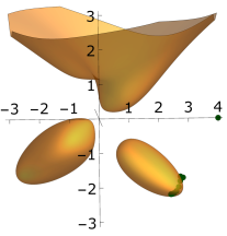
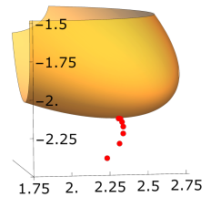
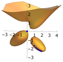
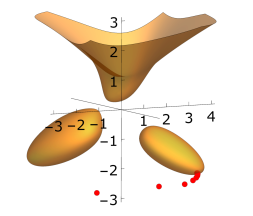
The transformation of the polynomial optimization to QCQP is standard and it is described in Appendix A for completeness. The global optimal objective value of the above QCQP equals 2.01982.0198-2.0198 and the lower-bound, offered by the standard SDP relaxation equals 89.890189.8901-89.8901. In order to solve the above QCQP, we run Algorithm 1, equipped with the SDP relaxation (no additional valid inequalities) and penalty term η=0.025𝜂0.025\eta=0.025. The trajectory with three different initializations 𝒙^1=[0,0,0,0,0,0,0]superscript^𝒙1superscript0000000top\hat{\boldsymbol{x}}^{1}=[0,0,0,0,0,0,0]^{\top}, 𝒙^2=[3,0,2,9,0,4,0,27]superscript^𝒙2superscript302904027top\hat{\boldsymbol{x}}^{2}=[-3,0,2,9,0,4,0,27]^{\top}, and 𝒙^3=[0,4,0,0,16,0,0,0]superscript^𝒙3superscript040016000top\hat{\boldsymbol{x}}^{3}=[0,4,0,0,16,0,0,0]^{\top} are given in Table 1 and shown in Fig. 1. In all three cases, the algorithm achieves feasibility in 1–8 rounds. Moreover, a feasible solution with less than 0.2%percent0.20.2\% gap from global optimality is attained within 10 rounds in all three cases. The example illustrates a case for which the heuristic Algorithm 1 is not sensitive to the choice of initial point.
Refer to caption
Refer to caption
Refer to caption
Refer to caption
Refer to caption
Refer to caption
Figure 1: Trajectory of Algorithm 1 for three different initializations. The yellow surface represents the feasible set and the , red and green points correspond to 𝒙^1superscript^𝒙1\hat{\boldsymbol{x}}^{1}, 𝒙^2superscript^𝒙2\hat{\boldsymbol{x}}^{2} and 𝒙^3superscript^𝒙3\hat{\boldsymbol{x}}^{3}, respectively.
Table 1: Trajectory of Algorithm 1 for three different initializations.
Round 𝒙^1superscript^𝒙1\hat{\boldsymbol{x}}^{1} 𝒙^2superscript^𝒙2\hat{\boldsymbol{x}}^{2} 𝒙^3superscript^𝒙3\hat{\boldsymbol{x}}^{3}
a𝑎a (obj.) b𝑏b c𝑐c

tr{𝑿𝒙𝒙}tr𝑿𝒙superscript𝒙top\mathrm{tr}\{\accentset{\ast}{\boldsymbol{X}}-\accentset{\ast}{\boldsymbol{x}}\accentset{\ast}{\boldsymbol{x}}^{\top}\}

a𝑎a (obj.) b𝑏b c𝑐c

tr{𝑿𝒙𝒙}tr𝑿𝒙superscript𝒙top\mathrm{tr}\{\accentset{\ast}{\boldsymbol{X}}-\accentset{\ast}{\boldsymbol{x}}\accentset{\ast}{\boldsymbol{x}}^{\top}\}

a𝑎a (obj.) b𝑏b c𝑐c

tr{𝑿𝒙𝒙}tr𝑿𝒙superscript𝒙top\mathrm{tr}\{\accentset{\ast}{\boldsymbol{X}}-\accentset{\ast}{\boldsymbol{x}}\accentset{\ast}{\boldsymbol{x}}^{\top}\}

0 0.0000 0.0000 0.0000 - -3.0000 0.0000 2.0000 - 0.0000 4.0000 0.0000 -
1 -1.2739 0.6601 -0.4697 2.1884 -2.5377 1.2831 -0.7380 138.9796 -1.5721 2.6848 -0.9492 39.2455
2 -1.5173 1.1445 -1.0128 <1011absentsuperscript1011<10^{-11} -2.4389 2.0715 -1.3946 51.1170 -1.5749 2.7588 -1.3854 13.5140
3 -1.6882 1.3773 -1.2015 <1011absentsuperscript1011<10^{-11} -2.2889 2.2685 -1.7098 23.0050 -1.6678 2.6583 -1.5228 0.9995
4 -1.8021 1.5739 -1.3561 <1011absentsuperscript1011<10^{-11} -2.1878 2.3416 -1.8442 11.4963 -1.8322 2.6083 -1.5587 <1011absentsuperscript1011<10^{-11}
5 -1.8824 1.7447 -1.4873 <1011absentsuperscript1011<10^{-11} -2.1194 2.3621 -1.9007 5.9206 -1.9460 2.5261 -1.6624 <1011absentsuperscript1011<10^{-11}
6 -1.9386 1.8930 -1.5992 <1011absentsuperscript1011<10^{-11} -2.0733 2.3611 -1.9250 2.9082 -2.0002 2.4391 -1.7847 <1011absentsuperscript1011<10^{-11}
7 -1.9760 2.0180 -1.6923 <1011absentsuperscript1011<10^{-11} -2.0423 2.3526 -1.9352 1.1594 -2.0156 2.3824 -1.8598 <1011absentsuperscript1011<10^{-11}
8 -1.9985 2.1175 -1.7656 <1011absentsuperscript1011<10^{-11} -2.0214 2.3426 -1.9393 0.0938 -2.0189 2.3532 -1.8938 <1011absentsuperscript1011<10^{-11}
9 -2.0104 2.1907 -1.8193 <1011absentsuperscript1011<10^{-11} -2.0197 2.3352 -1.9302 <1011absentsuperscript1011<10^{-11} -2.0196 2.3387 -1.9079 <1011absentsuperscript1011<10^{-11}
10 -2.0160 2.2408 -1.8559 <1011absentsuperscript1011<10^{-11} -2.0198 2.3304 -1.9240 <1011absentsuperscript1011<10^{-11} -2.0197 2.3313 -1.9135 <1011absentsuperscript1011<10^{-11}

4 Numerical experiments

In this section we describe numerical experiments to test the effectiveness of the sequential penalization method for non-convex QCQPs from the library of quadratic programming instances (QPLIB) Furini et al. (2019) as well as large-scale system identification problems Fattahi and Sojoudi (2018).

4.1 QPLIB problems

The experiments are performed on a desktop computer with a 12-core 3.0GHz CPU and 256GB RAM. MOSEK v8.1 ApS (2017) is used through MATLAB 2017a to solve the resulting SDPs. The size and number of constraints for each QPLIB instance are reported in Table 2.

4.1.1 Sequential penalization

Tables 3, 4, 5, and 6 report the results of Algorithm 1 for 2×2222\times 2 SDP, 2×2222\times 2 SDP+RLT, SDP, and SDP+RLT relaxations, respectively. The following valid inequalities are imposed on all of the convex relaxations:

Xkk(xklb+xkub)xk+xklbxkub0,subscript𝑋𝑘𝑘subscriptsuperscript𝑥lb𝑘subscriptsuperscript𝑥ub𝑘subscript𝑥𝑘subscriptsuperscript𝑥lb𝑘subscriptsuperscript𝑥ub𝑘0\displaystyle X_{kk}-(x^{\mathrm{lb}\!\!\!\!\!\phantom{\mathrm{ub}}}_{k}+x^{\mathrm{ub}\!\!\!\!\!\phantom{\mathrm{lb}}}_{k})x_{k}+x^{\mathrm{lb}\!\!\!\!\!\phantom{\mathrm{ub}}}_{k}x^{\mathrm{ub}\!\!\!\!\!\phantom{\mathrm{lb}}}_{k}\leq 0, k{1,,n}for-all𝑘1𝑛\displaystyle\qquad\forall k\in\{1,\ldots,n\} (43a)
Xkk(xkub+xkub)xk+xkubxkub0,subscript𝑋𝑘𝑘subscriptsuperscript𝑥ub𝑘subscriptsuperscript𝑥ub𝑘subscript𝑥𝑘subscriptsuperscript𝑥ub𝑘subscriptsuperscript𝑥ub𝑘0\displaystyle X_{kk}-(x^{\mathrm{ub}\!\!\!\!\!\phantom{\mathrm{lb}}}_{k}+x^{\mathrm{ub}\!\!\!\!\!\phantom{\mathrm{lb}}}_{k})x_{k}+x^{\mathrm{ub}\!\!\!\!\!\phantom{\mathrm{lb}}}_{k}x^{\mathrm{ub}\!\!\!\!\!\phantom{\mathrm{lb}}}_{k}\geq 0, k{1,,n}for-all𝑘1𝑛\displaystyle\qquad\forall k\in\{1,\ldots,n\} (43b)
Xkk(xklb+xklb)xk+xklbxklb0,subscript𝑋𝑘𝑘subscriptsuperscript𝑥lb𝑘subscriptsuperscript𝑥lb𝑘subscript𝑥𝑘subscriptsuperscript𝑥lb𝑘subscriptsuperscript𝑥lb𝑘0\displaystyle X_{kk}-(x^{\mathrm{lb}\!\!\!\!\!\phantom{\mathrm{ub}}}_{k}+x^{\mathrm{lb}\!\!\!\!\!\phantom{\mathrm{ub}}}_{k})x_{k}+x^{\mathrm{lb}\!\!\!\!\!\phantom{\mathrm{ub}}}_{k}x^{\mathrm{lb}\!\!\!\!\!\phantom{\mathrm{ub}}}_{k}\geq 0, k{1,,n}for-all𝑘1𝑛\displaystyle\qquad\forall k\in\{1,\ldots,n\} (43c)

where 𝒙lb,𝒙ubnsuperscript𝒙lbsuperscript𝒙ubsuperscript𝑛\boldsymbol{x}^{\mathrm{lb}},\boldsymbol{x}^{\mathrm{ub}}\in\mathbb{R}^{n} are given lower and upper bounds on 𝒙𝒙\boldsymbol{x}. Problem (4a)–(4d) is solved with the following four settings:

  • 2×2222\times 2 SDP relaxation: r=2𝑟2r=2 and valid inequalities (43a) – (43c).

  • 2×2222\times 2 SDP+RLT relaxation: 𝒱=×𝒱\mathcal{V}=\mathcal{H}\times\mathcal{H} and r=2𝑟2r=2.

  • SDP relaxation: r=n𝑟𝑛r=n and valid inequalities (43a) – (43c).

  • SDP+RLT relaxation: 𝒱=×𝒱\mathcal{V}=\mathcal{H}\times\mathcal{H} and r=n𝑟𝑛r=n,

where 𝒱𝒱\mathcal{V} and \mathcal{H} is defined in Appendix B. The assumption 𝒱=×𝒱\mathcal{V}=\mathcal{H}\times\mathcal{H} means that every pairs of linear constraints are used to generate RLT inequalities. Let (𝒙,𝑿)𝒙𝑿(\accentset{\ast}{\boldsymbol{x}},\accentset{\ast}{\boldsymbol{X}}) denote the optimal solution of the convex relaxation (4a)-(4d). We use the point 𝒙^=𝒙^𝒙𝒙\hat{\boldsymbol{x}}=\accentset{\ast}{\boldsymbol{x}} as the initial point of the algorithm.

The penalty parameter η𝜂\eta is chosen via bisection as the smallest number of the form α×10β𝛼superscript10𝛽\alpha\times 10^{\beta}, which results in a tight penalization during the first six rounds, where α{1,2,5}𝛼125\alpha\in\{1,2,5\} and β𝛽\beta is an integer. In all of the experiments, the value of η𝜂\eta has remained static throughout Algorithm 1. Denote the sequence of penalized SDP solutions obtained by Algorithm 1 as

(𝒙(1),𝑿(1)),(𝒙(2),𝑿(2)),(𝒙(3),𝑿(3)),superscript𝒙1superscript𝑿1superscript𝒙2superscript𝑿2superscript𝒙3superscript𝑿3\displaystyle(\boldsymbol{x}^{(1)},\boldsymbol{X}^{(1)}),\;\;(\boldsymbol{x}^{(2)},\boldsymbol{X}^{(2)}),\;\;(\boldsymbol{x}^{(3)},\boldsymbol{X}^{(3)}),\;\;\ldots

The smallest i𝑖i such that

tr{𝑿(i)𝒙(i)(𝒙(i))}<107trsuperscript𝑿𝑖superscript𝒙𝑖superscriptsuperscript𝒙𝑖topsuperscript107\displaystyle\mathrm{tr}\{\boldsymbol{X}^{(i)}-\boldsymbol{x}^{(i)}(\boldsymbol{x}^{(i)})^{\top}\}<10^{-7} (44)

is denoted by ifeassuperscript𝑖feasi^{\mathrm{feas}}, i.e., it is the number of rounds that Algorithm 1 needs to attain a tight penalization. Moreover, the smallest i𝑖i such that

q0(𝒙(i1))q0(𝒙(i))|q0(𝒙(i))|5×10⁴subscript𝑞0superscript𝒙𝑖1subscript𝑞0superscript𝒙𝑖subscript𝑞0superscript𝒙𝑖5superscript104\displaystyle\frac{q_{0}(\boldsymbol{x}^{(i-1)})-q_{0}(\boldsymbol{x}^{(i)})}{|q_{0}(\boldsymbol{x}^{(i)})|}\leq 5\times 10^{-4} (45)

is denoted by istopsuperscript𝑖stopi^{\mathrm{stop}}, and UBq0(𝒙(istop))UBsubscript𝑞0superscript𝒙superscript𝑖stop\mathrm{UB}\triangleq q_{0}(\boldsymbol{x}^{(i^{\mathrm{stop}})}). The following formula is used to calculate the final percentage gaps from the optimal costs reported by the QPLIB library:

GAP(%)\displaystyle\mathrm{GAP}(\%) =100×q0stopq0(𝒙QPLIB)|q0(𝒙QPLIB)|.absent100superscriptsubscript𝑞0stopsubscript𝑞0superscript𝒙QPLIBsubscript𝑞0superscript𝒙QPLIB\displaystyle=100\times\frac{q_{0}^{\mathrm{stop}}-q_{0}(\boldsymbol{x}^{\mathrm{QPLIB}})}{|q_{0}(\boldsymbol{x}^{\mathrm{QPLIB}})|}.\!\!\! (46)

Moreover, t𝑡t(s) denotes the cumulative solver time in seconds for the istopsuperscript𝑖stopi^{\mathrm{stop}} rounds. Our results are compared with BARON Tawarmalani and Sahinidis (2005) and COUENNE Belotti (2013) by fixing the maximum solver times equal to the accumulative solver times spent by Algorithm 1. We ran BARON and COUENNE through GAMS v25.1.2 GAMS Development Corporation (2013). The resulting lower bounds, upper bounds and GAPs (from the equation (46)) are reported in Tables 3, 4, 5, and 6.

Table 2: QPLIB benchmark problems.
​​​Inst​​​ Total Quad Total ​​​Inst​​​ Total Quad Total ​​​Inst​​​ Total Quad Total ​​​Inst​​​ Total Quad Total
Var Cons Cons Var Cons Cons Var Cons Cons Var Cons Cons
​​​ 0343 ​​​ 50 0 1 ​​​ 1353 ​​​ 50 1 6 ​​​ 1535 ​​​ 60 60 66 ​​​ 1773 ​​​ 60 1 7
​​​ 0911 ​​​ 50 50 50 ​​​ 1423 ​​​ 40 20 24 ​​​ 1619 ​​​ 50 25 30 ​​​ 1886 ​​​ 50 50 50
​​​ 0975 ​​​ 50 10 10 ​​​ 1437 ​​​ 50 1 11 ​​​ 1661 ​​​ 60 1 13 ​​​ 1913 ​​​ 48 48 48
​​​ 1055 ​​​ 40 20 20 ​​​ 1451 ​​​ 60 60 66 ​​​ 1675 ​​​ 60 1 13 ​​​ 1922 ​​​ 30 60 60
​​​ 1143 ​​​ 40 20 24 ​​​ 1493 ​​​ 40 1 5 ​​​ 1703 ​​​ 60 30 36 ​​​ 1931 ​​​ 40 40 40
​​​ 1157 ​​​ 40 1 9 ​​​ 1507 ​​​ 30 30 33 ​​​ 1745 ​​​ 50 50 55 ​​​ 1967 ​​​ 50 75 75
Table 3: Sequential penalized 2×2222\times 2 SDP.
​​​Inst​​​ Sequential penalized 2×2222\times 2 SDP BARON COUENNE
η𝜂\eta i\scaletofeas6ptsuperscript𝑖\scaletofeas6𝑝𝑡i^{\scaleto{\mathrm{feas}\mathstrut}{6pt}} i\scaletostop6ptsuperscript𝑖\scaletostop6𝑝𝑡i^{\scaleto{\mathrm{stop}\mathstrut}{6pt}} t𝑡t(s) UB GAP(%)​​​ LB UB GAP(%)​​​ LB UB GAP(%)​​​
​​​​ 0343\dagger ​​​​ ​​ ​​​ 5e+2 ​​​​​ ​​​​​​​​ 1 ​​​​​ ​​​​​​ 100 ​​​​​ ​​​​​​ 75.27 ​​​​​ ​​ -5.882 ​​​​​ ​​​​​​ 7.89 ​​​​​ ​​​​ ​ -95.372 ​​​ ​​​ -6.386 ​​​ ​​​​​​ 0.00 ​​​​​ ​​​​ ​ -7668.005 ​​​​​ ​​​ -6.386 ​​​ ​​​​​​ 0.00 ​​​​​​​​​
​​​​ 0911 ​​​​ ​​ ​​​ 1e+1 ​​​​​ ​​​​​​​​ 1 ​​​​​ ​​​​​​ 29 ​​​​​ ​​​​​​ 22.91 ​​​​​ ​​ -30.675 ​​​​​ ​​​​​​ 4.58 ​​​​​ ​​​​ ​ -172.777 ​​​ ​​​ 0.000 ​​​ ​​​​​​ 100 ​​​​​ ​​​​ ​ -172.777 ​​​ ​​​ -31.026 ​​​ ​​​​​​ 3.49 ​​​​​​​​​
​​​​ 0975 ​​​​ ​​ ​​​ 5e+0 ​​​​​ ​​​​​​​​ 6 ​​​​​ ​​​​​​ 18 ​​​​​ ​​​​​​ 46.36 ​​​​​ ​​ -36.434 ​​​​​ ​​​​​​ 3.75 ​​​​​ ​​​​ ​ -47.428 ​​​ ​​​ -37.801 ​​​ ​​​​​​ 0.14 ​​​​​ ​​​​ ​ -171.113 ​​​ ​​​ -37.213 ​​​ ​​​​​​ 1.69 ​​​​​​​​​
​​​​ 1055 ​​​​ ​​ ​​​ 1e+1 ​​​​​ ​​​​​​​​ 1 ​​​​​ ​​​​​​ 22 ​​​​​ ​​​​​​ 14.39 ​​​​​ ​​ -32.620 ​​​​​ ​​​​​​ 1.26 ​​​​​ ​​​​ ​ -37.841 ​​​ ​​​ -33.037 ​​​ ​​​​​​ 0.00 ​​​​​ ​​​​ ​ -199.457 ​​​ ​​​ -33.037 ​​​ ​​​​​​ 0.00 ​​​​​​​​​
​​​​ 1143 ​​​​ ​​ ​​​ 2e+1 ​​​​​ ​​​​​​​​ 1 ​​​​​ ​​​​​​ 44 ​​​​​ ​​​​​​ 25.68 ​​​​​ ​​ -55.417 ​​​​​ ​​​​​​ 3.20 ​​​​​ ​​​​ ​ -69.522 ​​​ ​​​ -57.247 ​​​ ​​​​​​ 0.00 ​​​​​ ​​​​ ​ -384.45 ​​​ ​​​ -56.237 ​​​ ​​​​​​ 1.76 ​​​​​​​​​
​​​​ 1157 ​​​​ ​​ ​​​ 2e+0 ​​​​​ ​​​​​​​​ 2 ​​​​​ ​​​​​​ 9 ​​​​​ ​​​​​​ 9.01 ​​​​​ ​​ -10.938 ​​​​​ ​​​​​​ 0.10 ​​​​​ ​​​​ ​ -11.414 ​​​ ​​​ -10.948 ​​​ ​​​​​​ 0.00 ​​​​​ ​​​​ ​ -80.51 ​​​ ​​​ -10.948 ​​​ ​​​​​​ 0.00 ​​​​​​​​​
​​​​ 1353 ​​​​ ​​ ​​​ 5e+0 ​​​​​ ​​​​​​​​ 1 ​​​​​ ​​​​​​ 48 ​​​​​ ​​​​​​ 84.90 ​​​​​ ​​ -7.700 ​​​​​ ​​​​​​ 0.19 ​​​​​ ​​​​ ​ -7.925 ​​​ ​​​ -7.714 ​​​ ​​​​​​ 0.00 ​​​​​ ​​​​ ​ -73.28 ​​​ ​​​ -7.714 ​​​ ​​​​​​ 0.00 ​​​​​​​​​
​​​​ 1423 ​​​​ ​​ ​​​ 5e+0 ​​​​​ ​​​​​​​​ 1 ​​​​​ ​​​​​​ 29 ​​​​​ ​​​​​​ 17.44 ​​​​​ ​​ -14.684 ​​​​​ ​​​​​​ 1.90 ​​​​​ ​​​​ ​ -16.313 ​​​ ​​​ -14.968 ​​​ ​​​​​​ 0.00 ​​​​​ ​​​​ ​ -76.13 ​​​ ​​​ -14.871 ​​​ ​​​​​​ 0.65 ​​​​​​​​​
​​​​ 1437 ​​​​ ​​ ​​​ 5e+0 ​​​​​ ​​​​​​​​ 1 ​​​​​ ​​​​​​ 36 ​​​​​ ​​​​​​ 54.57 ​​​​​ ​​ -7.785 ​​​​​ ​​​​​​ 0.06 ​​​​​ ​​​​ ​ -9.601 ​​​ ​​​ -7.789 ​​​ ​​​​​​ 0.00 ​​​​​ ​​​​ ​ -87.58 ​​​ ​​​ -7.789 ​​​ ​​​​​​ 0.00 ​​​​​​​​​
​​​​ 1451 ​​​​ ​​ ​​​ 2e+1 ​​​​​ ​​​​​​​​ 4 ​​​​​ ​​​​​​ 21 ​​​​​ ​​​​​​ 20.86 ​​​​​ ​​ -85.598 ​​​​​ ​​​​​​ 2.26 ​​​​​ ​​​​ ​ -135.140 ​​​ ​​​ -87.577 ​​​ ​​​​​​ 0.00 ​​​​​ ​​​​ ​ -468.04 ​​​ ​​​ -86.860 ​​​ ​​​​​​ 0.82 ​​​​​​​​​
​​​​ 1493 ​​​​ ​​ ​​​ 2e+1 ​​​​​ ​​​​​​​​ 1 ​​​​​ ​​​​​​ 18 ​​​​​ ​​​​​​ 14.49 ​​​​​ ​​ -41.910 ​​​​​ ​​​​​​ 2.90 ​​​​​ ​​​​ ​ -47.239 ​​​ ​​​ -43.160 ​​​ ​​​​​​ 0.00 ​​​​​ ​​​​ ​ -395.69 ​​​ ​​​ -43.160 ​​​ ​​​​​​ 0.00 ​​​​​​​​​
​​​​ 1507 ​​​​ ​​ ​​​​ 2e+0 ​​​​​ ​​​​​​​​ 1 ​​​​​ ​​​​​​ 15 ​​​​​ ​​​​​​ 8.98 ​​​​​ ​​ -8.289 ​​​​​ ​​​​​​ 0.15 ​​​​​ ​​​​ ​ -49.709 ​​​ ​​​ -8.301 ​​​ ​​​​​​ 0.00 ​​​​​ ​​​​ ​ -44.37 ​​​ ​​​ -8.301 ​​​ ​​​​​​ 0.00 ​​​​​​​​​
​​​​ 1535 ​​​​ ​​ ​​​ 5e+0 ​​​​​ ​​​​​​​​ 1 ​​​​​ ​​​​​​ 26 ​​​​​ ​​​​​​ 28.16 ​​​​​ ​​ -10.948 ​​​​​ ​​​​​​ 5.51 ​​​​​ ​​​​ ​ -13.407 ​​​ ​​​ -11.397 ​​​ ​​​​​​ 1.63 ​​​​​ ​​​​ ​ -107.86 ​​​ ​​​ -11.398 ​​​ ​​​​​​ 1.63 ​​​​​​​​​
​​​​ 1619 ​​​​ ​​ ​​​ 5e+0 ​​​​​ ​​​​​​​​ 1 ​​​​​ ​​​​​​ 39 ​​​​​ ​​​​​​ 32.34 ​​​​​ ​​ -9.210 ​​​​​ ​​​​​​ 0.08 ​​​​​ ​​​​ ​ -10.302 ​​​ ​​​ -9.217 ​​​ ​​​​​​ 0.00 ​​​​​ ​​​​ ​ -74.55 ​​​ ​​​ -9.217 ​​​ ​​​​​​ 0.00 ​​​​​​​​​
​​​​ 1661 ​​​​ ​​ ​​​ 5e+0 ​​​​​ ​​​​​​​​ 1 ​​​​​ ​​​​​​ 32 ​​​​​ ​​​​​​ 87.50 ​​​​​ ​​ -15.666 ​​​​​ ​​​​​​ 1.81 ​​​​​ ​​​​ ​ -19.667 ​​​ ​​​ -15.955 ​​​ ​​​​​​ 0.00 ​​​​​ ​​​​ ​ -139.25 ​​​ ​​​ -15.955 ​​​ ​​​​​​ 0.00 ​​​​​​​​​
​​​​ 1675 ​​​​ ​​ ​​​ 2e+1 ​​​​​ ​​​​​​​​ 1 ​​​​​ ​​​​​​ 21 ​​​​​ ​​​​​​ 36.38 ​​​​​ ​​ -75.485 ​​​​​ ​​​​​​ 0.24 ​​​​​ ​​​​ ​ -96.864 ​​​ ​​​ -75.669 ​​​ ​​​​​​ 0.00 ​​​​​ ​​​​ ​ -435.48 ​​​ ​​​ -75.669 ​​​ ​​​​​​ 0.00 ​​​​​​​​​
​​​​ 1703 ​​​​ ​​ ​​​ 5e+1 ​​​​​ ​​​​​​​​ 2 ​​​​​ ​​​​​​ 30 ​​​​​ ​​​​​​ 31.82 ​​​​​ ​​ -130.902 ​​​​​ ​​​​​​ 1.43 ​​​​​ ​​​​ ​ -180.935 ​​​ ​​​ -132.802 ​​​ ​​​​​​ 0.00 ​​​​​ ​​​​ ​ -929.92 ​​​ ​​​ -132.802 ​​​ ​​​​​​ 0.00 ​​​​​​​​​
​​​​ 1745 ​​​​ ​​ ​​​ 2e+1 ​​​​​ ​​​​​​​​ 1 ​​​​​ ​​​​​​ 26 ​​​​​ ​​​​​​ 22.15 ​​​​​ ​​ -71.704 ​​​​​ ​​​​​​ 0.93 ​​​​​ ​​​​ ​ -77.465 ​​​ ​​​ -72.377 ​​​ ​​​​​​ 0.00 ​​​​​ ​​​​ ​ -317.99 ​​​ ​​​ -72.377 ​​​ ​​​​​​ 0.00 ​​​​​​​​​
​​​​ 1773 ​​​​ ​​ ​​​ 5e+0 ​​​​​ ​​​​​​​​ 1 ​​​​​ ​​​​​​ 56 ​​​​​ ​​​​​​ 148.79 ​​​​​ ​​ -14.154 ​​​​​ ​​​​​​ 3.34 ​​​​​ ​​​​ ​ -21.581 ​​​ ​​​ -14.642 ​​​ ​​​​​​ 0.00 ​​​​​ ​​​​ ​ -118.65 ​​​ ​​​ -14.642 ​​​ ​​​​​​ 0.00 ​​​​​​​​​
​​​​ 1886 ​​​​ ​​ ​​​ 2e+1 ​​​​​ ​​​​​​​​ 1 ​​​​​ ​​​​​​ 34 ​​​​​ ​​​​​​ 26.82 ​​​​​ ​​ -78.604 ​​​​​ ​​​​​​ 0.09 ​​​​​ ​​​​ ​ -135.615 ​​​ ​​​ -78.672 ​​​ ​​​​​​ 0.00 ​​​​​ ​​​​ ​ -324.87 ​​​ ​​​ -78.672 ​​​ ​​​​​​ 0.00 ​​​​​​​​​
​​​​ 1913 ​​​​ ​​ ​​​ 1e+1 ​​​​​ ​​​​​​​​ 1 ​​​​​ ​​​​​​ 28 ​​​​​ ​​​​​​ 21.91 ​​​​​ ​​ -51.889 ​​​​​ ​​​​​​ 0.42 ​​​​​ ​​​​ ​ -68.555 ​​​ ​​​ -52.109 ​​​ ​​​​​​ 0.00 ​​​​​ ​​​​ ​ -164.26 ​​​ ​​​ -51.478 ​​​ ​​​​​​ 1.21 ​​​​​​​​​
​​​​ 1922 ​​​​ ​​ ​​​ 1e+1 ​​​​​ ​​​​​​​​ 1 ​​​​​ ​​​​​​ 23 ​​​​​ ​​​​​​ 11.16 ​​​​​ ​​ -35.437 ​​​​​ ​​​​​​ 1.43 ​​​​​ ​​​​ ​ -121.872 ​​​ ​​​ -35.951 ​​​ ​​​​​​ 0.00 ​​​​​ ​​​​ ​ -123.2 ​​​ ​​​ -35.951 ​​​ ​​​​​​ 0.00 ​​​​​​​​​
​​​​ 1931 ​​​​ ​​ ​​​ 1e+1 ​​​​​ ​​​​​​​​ 1 ​​​​​ ​​​​​​ 13 ​​​​​ ​​​​​​ 8.78 ​​​​​ ​​ -53.684 ​​​​​ ​​​​​​ 3.64 ​​​​​ ​​​​ ​ -85.196 ​​​ ​​​ -55.709 ​​​ ​​​​​​ 0.00 ​​​​​ ​​​​ ​ -204.08 ​​​ ​​​ -54.290 ​​​ ​​​​​​ 2.55 ​​​​​​​​​
​​​​ 1967 ​​​​ ​​ ​​​ 5e+1 ​​​​​ ​​​​​​​​ 1 ​​​​​ ​​​​​​ 32 ​​​​​ ​​​​​​ 27.23 ​​​​​ ​​ -105.570 ​​​​​ ​​​​​​ 1.87 ​​​​​ ​​​​ ​ -136.098 ​​​ ​​​ 0.000 ​​​ ​​​​​​ 100 ​​​​​ ​​​​ ​ -622.57 ​​​ ​​​ -107.581 ​​​ ​​​​​​ 0.00 ​​​​​​​​​
​​​​ Max ​​​​ ​​ ​​​ 500 ​​​​​ ​​​​​​​​ 6 ​​​​​ ​​​​​​ 100 ​​​​​ ​​​​​​ 148.79 ​​​​​ ​​​​​​ 7.89 ​​​​​ ​​​​​​ 100 ​​​​​ ​​​​​​ 3.34 ​​​​​​​​​
Table 4: Sequential penalized 2×2222\times 2 SDP+RLT.
​​​Inst​​​ Sequential 2×2222\times 2 SDP+RLT BARON COUENNE
η𝜂\eta i\scaletofeas6ptsuperscript𝑖\scaletofeas6𝑝𝑡i^{\scaleto{\mathrm{feas}\mathstrut}{6pt}} i\scaletostop6ptsuperscript𝑖\scaletostop6𝑝𝑡i^{\scaleto{\mathrm{stop}\mathstrut}{6pt}} t𝑡t(s) UB GAP(%)​​​ LB UB GAP(%)​​​ LB UB GAP(%)​​​
​​​​ 0343 ​​​​ ​​ ​​​ 1e+2 ​​​​​ ​​​​​​​​ 4 ​​​​​ ​​​​​​ 24 ​​​​​ ​​​​​​ 25.23 ​​​​​ ​​ -5.945 ​​​​​ ​​​​​​ 6.91 ​​​​​ ​​​​ ​ -95.372 ​​​ ​​​ -6.386 ​​​ ​​​​​​ 0.00 ​​​​​ ​​​​ ​ -7668.005 ​​​ ​​​ -6.386 ​​​ ​​​​​​ 0.00 ​​​​​​​​​
​​​​ 0911 ​​​​ ​​ ​​​ 1e+1 ​​​​​ ​​​​​​​​ 1 ​​​​​ ​​​​​​ 33 ​​​​​ ​​​​​​ 27.69 ​​​​​ ​​ -30.923 ​​​​​ ​​​​​​ 3.81 ​​​​​ ​​​​ ​ -172.777 ​​​ ​​​ -32.148 ​​​ ​​​​​​ 0.00 ​​​​​ ​​​​ ​ -172.777 ​​​ ​​​ -31.026 ​​​ ​​​​​​ 3.49 ​​​​​​​​​
​​​​ 0975 ​​​​ ​​ ​​​ 5e+0 ​​​​​ ​​​​​​​​ 6 ​​​​​ ​​​​​​ 15 ​​​​​ ​​​​​​ 4.10 ​​​​​ ​​ -36.300 ​​​​​ ​​​​​​ 13.17 ​​​​​ ​​​​ ​ -47.428 ​​​ ​​​ -37.794 ​​​ ​​​​​​ 0.16 ​​​​​ ​​​​ ​ -171.113 ​​​ ​​​ -36.812 ​​​ ​​​​​​ 2.75 ​​​​​​​​​
​​​​ 1055 ​​​​ ​​ ​​​ 1e+1 ​​​​​ ​​​​​​​​ 1 ​​​​​ ​​​​​​ 24 ​​​​​ ​​​​​​ 16.78 ​​​​​ ​​ -32.666 ​​​​​ ​​​​​​ 1.12 ​​​​​ ​​​​ ​ -37.841 ​​​ ​​​ -33.037 ​​​ ​​​​​​ 0.00 ​​​​​ ​​​​ ​ -199.457 ​​​ ​​​ -33.037 ​​​ ​​​​​​ 0.00 ​​​​​​​​​
​​​​ 1143 ​​​​ ​​ ​​​ 2e+1 ​​​​​ ​​​​​​​​ 1 ​​​​​ ​​​​​​ 30 ​​​​​ ​​​​​​ 32.66 ​​​​​ ​​ -55.507 ​​​​​ ​​​​​​ 3.04 ​​​​​ ​​​​ ​ -69.522 ​​​ ​​​ -57.247 ​​​ ​​​​​​ 0.00 ​​​​​ ​​​​ ​ -384.45 ​​​ ​​​ -56.237 ​​​ ​​​​​​ 1.76 ​​​​​​​​​
​​​​ 1157 ​​​​ ​​ ​​​ 2e+0 ​​​​​ ​​​​​​​​ 1 ​​​​​ ​​​​​​ 0 ​​​​​ ​​​​​​ 1.14 ​​​​​ ​​ -10.948 ​​​​​ ​​​​​​ 0.00 ​​​​​ ​​​​ ​ -11.414 ​​​ ​​​ -10.948 ​​​ ​​​​​​ 0.00 ​​​​​ ​​​​ ​ -80.51 ​​​ ​​​ -10.948 ​​​ ​​​​​​ 0.00 ​​​​​​​​​
​​​​ 1353 ​​​​ ​​ ​​​ 1e+0 ​​​​​ ​​​​​​​​ 3 ​​​​​ ​​​​​​ 11 ​​​​​ ​​​​​​ 19.41 ​​​​​ ​​ -7.711 ​​​​​ ​​​​​​ 0.05 ​​​​​ ​​​​ ​ -7.925 ​​​ ​​​ -7.714 ​​​ ​​​​​​ 0.00 ​​​​​ ​​​​ ​ -73.28 ​​​ ​​​ -7.714 ​​​ ​​​​​​ 0.00 ​​​​​​​​​
​​​​ 1423 ​​​​ ​​ ​​​ 2e+0 ​​​​​ ​​​​​​​​ 3 ​​​​​ ​​​​​​ 14 ​​​​​ ​​​​​​ 16.41 ​​​​​ ​​ -14.730 ​​​​​ ​​​​​​ 1.59 ​​​​​ ​​​​ ​ -16.313 ​​​ ​​​ -14.968 ​​​ ​​​​​​ 0.00 ​​​​​ ​​​​ ​ -76.13 ​​​ ​​​ -14.871 ​​​ ​​​​​​ 0.65 ​​​​​​​​​
​​​​ 1437 ​​​​ ​​ ​​​ 5e-1 ​​​​​ ​​​​​​​​ 4 ​​​​​ ​​​​​​ 8 ​​​​​ ​​​​​​ 21.62 ​​​​​ ​​ -7.788 ​​​​​ ​​​​​​ 0.02 ​​​​​ ​​​​ ​ -9.601 ​​​ ​​​ -7.789 ​​​ ​​​​​​ 0.00 ​​​​​ ​​​​ ​ -87.58 ​​​ ​​​ -7.789 ​​​ ​​​​​​ 0.00 ​​​​​​​​​
​​​​ 1451 ​​​​ ​​ ​​​ 2e+1 ​​​​​ ​​​​​​​​ 2 ​​​​​ ​​​​​​ 36 ​​​​​ ​​​​​​ 100.50 ​​​​​ ​​ -87.502 ​​​​​ ​​​​​​ 0.09 ​​​​​ ​​​​ ​ -135.140 ​​​ ​​​ -87.577 ​​​ ​​​​​​ 0.00 ​​​​​ ​​​​ ​ -468.04 ​​​ ​​​ -87.283 ​​​ ​​​​​​ 0.34 ​​​​​​​​​
​​​​ 1493 ​​​​ ​​ ​​​ 1e+1 ​​​​​ ​​​​​​​​ 3 ​​​​​ ​​​​​​ 13 ​​​​​ ​​​​​​ 13.69 ​​​​​ ​​ -41.804 ​​​​​ ​​​​​​ 3.14 ​​​​​ ​​​​ ​ -47.239 ​​​ ​​​ -43.160 ​​​ ​​​​​​ 0.00 ​​​​​ ​​​​ ​ -395.69 ​​​ ​​​ -43.160 ​​​ ​​​​​​ 0.00 ​​​​​​​​​
​​​​ 1507 ​​​​ ​​ ​​​ 1e+0 ​​​​​ ​​​​​​​​ 6 ​​​​​ ​​​​​​ 13 ​​​​​ ​​​​​​ 10.31 ​​​​​ ​​ -8.295 ​​​​​ ​​​​​​ 0.08 ​​​​​ ​​​​ ​ -49.709 ​​​ ​​​ -8.301 ​​​ ​​​​​​ 0.00 ​​​​​ ​​​​ ​ -44.37 ​​​ ​​​ -8.301 ​​​ ​​​​​​ 0.00 ​​​​​​​​​
​​​​ 1535 ​​​​ ​​ ​​​ 2e+0 ​​​​​ ​​​​​​​​ 3 ​​​​​ ​​​​​​ 23 ​​​​​ ​​​​​​ 83.47 ​​​​​ ​​ -11.241 ​​​​​ ​​​​​​ 2.98 ​​​​​ ​​​​ ​ -13.407 ​​​ ​​​ -11.586 ​​​ ​​​​​​ 0.00 ​​​​​ ​​​​ ​ -107.86 ​​​ ​​​ -11.398 ​​​ ​​​​​​ 1.62 ​​​​​​​​​
​​​​ 1619 ​​​​ ​​ ​​​ 2e+0 ​​​​​ ​​​​​​​​ 3 ​​​​​ ​​​​​​ 20 ​​​​​ ​​​​​​ 35.62 ​​​​​ ​​ -9.213 ​​​​​ ​​​​​​ 0.05 ​​​​​ ​​​​ ​ -10.302 ​​​ ​​​ -9.217 ​​​ ​​​​​​ 0.00 ​​​​​ ​​​​ ​ -74.55 ​​​ ​​​ -9.217 ​​​ ​​​​​​ 0.00 ​​​​​​​​​
​​​​ 1661 ​​​​ ​​ ​​​ 1e+0 ​​​​​ ​​​​​​​​ 3 ​​​​​ ​​​​​​ 8 ​​​​​ ​​​​​​ 35.85 ​​​​​ ​​ -15.666 ​​​​​ ​​​​​​ 1.81 ​​​​​ ​​​​ ​ -19.667 ​​​ ​​​ -15.955 ​​​ ​​​​​​ 0.00 ​​​​​ ​​​​ ​ -139.25 ​​​ ​​​ -15.955 ​​​ ​​​​​​ 0.00 ​​​​​​​​​
​​​​ 1675 ​​​​ ​​ ​​​ 1e+1 ​​​​​ ​​​​​​​​ 3 ​​​​​ ​​​​​​ 11 ​​​​​ ​​​​​​ 41.30 ​​​​​ ​​ -75.537 ​​​​​ ​​​​​​ 0.17 ​​​​​ ​​​​ ​ -96.864 ​​​ ​​​ -75.669 ​​​ ​​​​​​ 0.00 ​​​​​ ​​​​ ​ -435.48 ​​​ ​​​ -75.669 ​​​ ​​​​​​ 0.00 ​​​​​​​​​
​​​​ 1703 ​​​​ ​​ ​​​ 2e+1 ​​​​​ ​​​​​​​​ 5 ​​​​​ ​​​​​​ 22 ​​​​​ ​​​​​​ 62.63 ​​​​​ ​​ -131.330 ​​​​​ ​​​​​​ 1.11 ​​​​​ ​​​​ ​ -180.935 ​​​ ​​​ -132.802 ​​​ ​​​​​​ 0.00 ​​​​​ ​​​​ ​ -929.92 ​​​ ​​​ -132.802 ​​​ ​​​​​​ 0.00 ​​​​​​​​​
​​​​ 1745 ​​​​ ​​ ​​​ 5e+0 ​​​​​ ​​​​​​​​ 4 ​​​​​ ​​​​​​ 19 ​​​​​ ​​​​​​ 40.44 ​​​​​ ​​ -72.351 ​​​​​ ​​​​​​ 0.04 ​​​​​ ​​​​ ​ -77.465 ​​​ ​​​ -72.377 ​​​ ​​​​​​ 0.00 ​​​​​ ​​​​ ​ -317.99 ​​​ ​​​ -72.377 ​​​ ​​​​​​ 0.00 ​​​​​​​​​
​​​​ 1773 ​​​​ ​​ ​​​ 5e+0 ​​​​​ ​​​​​​​​ 1 ​​​​​ ​​​​​​ 56 ​​​​​ ​​​​​​ 120.65 ​​​​​ ​​ -14.176 ​​​​​ ​​​​​​ 3.19 ​​​​​ ​​​​ ​ -21.581 ​​​ ​​​ -14.642 ​​​ ​​​​​​ 0.00 ​​​​​ ​​​​ ​ -118.65 ​​​ ​​​ -14.642 ​​​ ​​​​​​ 0.00 ​​​​​​​​​
​​​​ 1886 ​​​​ ​​ ​​​ 2e+1 ​​​​​ ​​​​​​​​ 1 ​​​​​ ​​​​​​ 35 ​​​​​ ​​​​​​ 28.19 ​​​​​ ​​ -78.620 ​​​​​ ​​​​​​ 0.07 ​​​​​ ​​​​ ​ -135.615 ​​​ ​​​ -78.672 ​​​ ​​​​​​ 0.00 ​​​​​ ​​​​ ​ -324.87 ​​​ ​​​ -78.672 ​​​ ​​​​​​ 0.00 ​​​​​​​​​
​​​​ 1913 ​​​​ ​​ ​​​ 5e+0 ​​​​​ ​​​​​​​​ 4 ​​​​​ ​​​​​​ 18 ​​​​​ ​​​​​​ 15.10 ​​​​​ ​​ -51.879 ​​​​​ ​​​​​​ 0.44 ​​​​​ ​​​​ ​ -68.555 ​​​ ​​​ -52.109 ​​​ ​​​​​​ 0.00 ​​​​​ ​​​​ ​ -164.26 ​​​ ​​​ -51.348 ​​​ ​​​​​​ 1.46 ​​​​​​​​​
​​​​ 1922 ​​​​ ​​ ​​​ 1e+1 ​​​​​ ​​​​​​​​ 1 ​​​​​ ​​​​​​ 26 ​​​​​ ​​​​​​ 13.22 ​​​​​ ​​ -35.451 ​​​​​ ​​​​​​ 1.39 ​​​​​ ​​​​ ​ -121.872 ​​​ ​​​ -35.951 ​​​ ​​​​​​ 0.00 ​​​​​ ​​​​ ​ -123.2 ​​​ ​​​ -35.951 ​​​ ​​​​​​ 0.00 ​​​​​​​​​
​​​​ 1931 ​​​​ ​​ ​​​ 1e+1 ​​​​​ ​​​​​​​​ 1 ​​​​​ ​​​​​​ 13 ​​​​​ ​​​​​​ 8.59 ​​​​​ ​​ -53.709 ​​​​​ ​​​​​​ 3.59 ​​​​​ ​​​​ ​ -85.196 ​​​ ​​​ -55.709 ​​​ ​​​​​​ 0.00 ​​​​​ ​​​​ ​ -204.08 ​​​ ​​​ -54.290 ​​​ ​​​​​​ 2.55 ​​​​​​​​​
​​​​ 1967 ​​​​ ​​ ​​​ 5e+1 ​​​​​ ​​​​​​​​ 1 ​​​​​ ​​​​​​ 38 ​​​​​ ​​​​​​ 33.01 ​​​​​ ​​ -105.616 ​​​​​ ​​​​​​ 1.83 ​​​​​ ​​​​ ​ -136.098 ​​​ ​​​ 0.000 ​​​ ​​​​​​ 100 ​​​​​ ​​​​ ​ -622.57 ​​​ ​​​ -107.581 ​​​ ​​​​​​ 0.00 ​​​​​​​​​
​​​​ Max ​​​​ ​​ ​​​ 100 ​​​​​ ​​​​​​​​ 6 ​​​​​ ​​​​​​ 56 ​​​​​ ​​​​​​ 120.65 ​​​​​ ​​​​​​ 13.17 ​​​​​ ​​​​​​ 100 ​​​​​ ​​​​​​ 3.49 ​​​​​​​​​
Table 5: Sequential penalized SDP.
​​​Inst​​​ Sequential SDP BARON COUENNE
η𝜂\eta i\scaletofeas6ptsuperscript𝑖\scaletofeas6𝑝𝑡i^{\scaleto{\mathrm{feas}\mathstrut}{6pt}} i\scaletostop6ptsuperscript𝑖\scaletostop6𝑝𝑡i^{\scaleto{\mathrm{stop}\mathstrut}{6pt}} t𝑡t(s) UB GAP(%)​​​ LB UB GAP(%)​​​ LB UB GAP(%)​​​
​​​​ 0343 ​​​​ ​​ ​​​ 1e+2 ​​​​​ ​​​​​​​​ 1 ​​​​​ ​​​​​​ 53 ​​​​​ ​​​​​​ 29.24 ​​​​​ ​​ -6.379 ​​​​​ ​​​​​​ 0.12 ​​​​​ ​​​​ ​ -95.372 ​​​ ​​​ -6.386 ​​​ ​​​​​​ 0.00 ​​​​​ ​​​​ ​ -7668.005 ​​​ ​​​ -6.386 ​​​ ​​​​​​ 0.00 ​​​​​​​​​
​​​​ 0911 ​​​​ ​​ ​​​ 2e+0 ​​​​​ ​​​​​​​​ 1 ​​​​​ ​​​​​​ 9 ​​​​​ ​​​​​​ 5.19 ​​​​​ ​​ -31.811 ​​​​​ ​​​​​​ 1.05 ​​​​​ ​​​​ ​ -172.777 ​​​ ​​​ 0.000 ​​​ ​​​​​​ 100 ​​​​​ ​​​​ ​ -172.777 ​​​ ​​​ -31.026 ​​​ ​​​​​​ 3.49 ​​​​​​​​​
​​​​ 0975 ​​​​ ​​ ​​​ 2e+0 ​​​​​ ​​​​​​​​ 2 ​​​​​ ​​​​​​ 13 ​​​​​ ​​​​​​ 8.18 ​​​​​ ​​ -37.845 ​​​​​ ​​​​​​ 0.02 ​​​​​ ​​​​ ​ -47.428 ​​​ ​​​ -37.794 ​​​ ​​​​​​ 0.16 ​​​​​ ​​​​ ​ -171.113 ​​​ ​​​ -36.812 ​​​ ​​​​​​ 2.75 ​​​​​​​​​
​​​​ 1055 ​​​​ ​​ ​​​ 5e+0 ​​​​​ ​​​​​​​​ 1 ​​​​​ ​​​​​​ 8 ​​​​​ ​​​​​​ 4.36 ​​​​​ ​​ -32.528 ​​​​​ ​​​​​​ 1.54 ​​​​​ ​​​​ ​ -37.841 ​​​ ​​​ -33.037 ​​​ ​​​​​​ 0.00 ​​​​​ ​​​​ ​ -199.457 ​​​ ​​​ -33.037 ​​​ ​​​​​​ 0.00 ​​​​​​​​​
​​​​ 1143 ​​​​ ​​ ​​​ 5e+0 ​​​​​ ​​​​​​​​ 4 ​​​​​ ​​​​​​ 15 ​​​​​ ​​​​​​ 7.89 ​​​​​ ​​ -55.606 ​​​​​ ​​​​​​ 2.87 ​​​​​ ​​​​ ​ -69.522 ​​​ ​​​ -57.247 ​​​ ​​​​​​ 0.00 ​​​​​ ​​​​ ​ -384.45 ​​​ ​​​ -53.367 ​​​ ​​​​​​ 6.78 ​​​​​​​​​
​​​​ 1157 ​​​​ ​​ ​​​ 1e+0 ​​​​​ ​​​​​​​​ 1 ​​​​​ ​​​​​​ 5 ​​​​​ ​​​​​​ 3.15 ​​​​​ ​​ -10.945 ​​​​​ ​​​​​​ 0.03 ​​​​​ ​​​​ ​ -11.414 ​​​ ​​​ -10.948 ​​​ ​​​​​​ 0.00 ​​​​​ ​​​​ ​ -80.51 ​​​ ​​​ -10.948 ​​​ ​​​​​​ 0.00 ​​​​​​​​​
​​​​ 1353 ​​​​ ​​ ​​​ 1e+0 ​​​​​ ​​​​​​​​ 1 ​​​​​ ​​​​​​ 10 ​​​​​ ​​​​​​ 6.12 ​​​​​ ​​ -7.712 ​​​​​ ​​​​​​ 0.03 ​​​​​ ​​​​ ​ -7.925 ​​​ ​​​ -7.714 ​​​ ​​​​​​ 0.00 ​​​​​ ​​​​ ​ -73.28 ​​​ ​​​ -7.714 ​​​ ​​​​​​ 0.00 ​​​​​​​​​
​​​​ 1423 ​​​​ ​​ ​​​ 1e+0 ​​​​​ ​​​​​​​​ 1 ​​​​​ ​​​​​​ 5 ​​​​​ ​​​​​​ 3.28 ​​​​​ ​​ -14.676 ​​​​​ ​​​​​​ 1.95 ​​​​​ ​​​​ ​ -16.313 ​​​ ​​​ -14.968 ​​​ ​​​​​​ 0.00 ​​​​​ ​​​​ ​ -76.13 ​​​ ​​​ -14.078 ​​​ ​​​​​​ 5.94 ​​​​​​​​​
​​​​ 1437 ​​​​ ​​ ​​​ 1e+0 ​​​​​ ​​​​​​​​ 1 ​​​​​ ​​​​​​ 7 ​​​​​ ​​​​​​ 4.30 ​​​​​ ​​ -7.787 ​​​​​ ​​​​​​ 0.03 ​​​​​ ​​​​ ​ -9.601 ​​​ ​​​ -7.789 ​​​ ​​​​​​ 0.00 ​​​​​ ​​​​ ​ -87.58 ​​​ ​​​ -7.789 ​​​ ​​​​​​ 0.00 ​​​​​​​​​
​​​​ 1451 ​​​​ ​​ ​​​ 5e+0 ​​​​​ ​​​​​​​​ 2 ​​​​​ ​​​​​​ 6 ​​​​​ ​​​​​​ 5.09 ​​​​​ ​​ -85.972 ​​​​​ ​​​​​​ 1.83 ​​​​​ ​​​​ ​ -135.140 ​​​ ​​​ - ​​​ ​​​​​​ - ​​​​​ ​​​​ ​ -468.04 ​​​ ​​​ - ​​​ ​​​​​​ - ​​​​​​​​​
​​​​ 1493 ​​​​ ​​ ​​​ 5e+0 ​​​​​ ​​​​​​​​ 1 ​​​​​ ​​​​​​ 6 ​​​​​ ​​​​​​ 4.10 ​​​​​ ​​ -43.160 ​​​​​ ​​​​​​ 0.00 ​​​​​ ​​​​ ​ -47.239 ​​​ ​​​ -43.160 ​​​ ​​​​​​ 0.00 ​​​​​ ​​​​ ​ -395.69 ​​​ ​​​ -43.160 ​​​ ​​​​​​ 0.00 ​​​​​​​​​
​​​​ 1507 ​​​​ ​​ ​​​ 5e-1 ​​​​​ ​​​​​​​​ 3 ​​​​​ ​​​​​​ 6 ​​​​​ ​​​​​​ 3.28 ​​​​​ ​​ -8.291 ​​​​​ ​​​​​​ 0.12 ​​​​​ ​​​​ ​ -49.709 ​​​ ​​​ -8.301 ​​​ ​​​​​​ 0.00 ​​​​​ ​​​​ ​ -44.37 ​​​ ​​​ -8.301 ​​​ ​​​​​​ 0.00 ​​​​​​​​​
​​​​ 1535 ​​​​ ​​ ​​​ 1e+0 ​​​​​ ​​​​​​​​ 1 ​​​​​ ​​​​​​ 16 ​​​​​ ​​​​​​ 13.05 ​​​​​ ​​ -11.363 ​​​​​ ​​​​​​ 1.93 ​​​​​ ​​​​ ​ -13.407 ​​​ ​​​ -11.397 ​​​ ​​​​​​ 1.63 ​​​​​ ​​​​ ​ -107.86 ​​​ ​​​ -11.398 ​​​ ​​​​​​ 1.63 ​​​​​​​​​
​​​​ 1619 ​​​​ ​​ ​​​ 1e+0 ​​​​​ ​​​​​​​​ 1 ​​​​​ ​​​​​​ 7 ​​​​​ ​​​​​​ 4.64 ​​​​​ ​​ -9.213 ​​​​​ ​​​​​​ 0.05 ​​​​​ ​​​​ ​ -10.302 ​​​ ​​​ -9.217 ​​​ ​​​​​​ 0.00 ​​​​​ ​​​​ ​ -74.55 ​​​ ​​​ -9.217 ​​​ ​​​​​​ 0.00 ​​​​​​​​​
​​​​ 1661 ​​​​ ​​ ​​​ 1e+0 ​​​​​ ​​​​​​​​ 1 ​​​​​ ​​​​​​ 12 ​​​​​ ​​​​​​ 7.57 ​​​​​ ​​ -15.955 ​​​​​ ​​​​​​ 0.00 ​​​​​ ​​​​ ​ -19.667 ​​​ ​​​ -15.955 ​​​ ​​​​​​ 0.00 ​​​​​ ​​​​ ​ -139.25 ​​​ ​​​ -15.955 ​​​ ​​​​​​ 0.00 ​​​​​​​​​
​​​​ 1675 ​​​​ ​​ ​​​ 5e+0 ​​​​​ ​​​​​​​​ 1 ​​​​​ ​​​​​​ 5 ​​​​​ ​​​​​​ 3.75 ​​​​​ ​​ -75.550 ​​​​​ ​​​​​​ 0.16 ​​​​​ ​​​​ ​ -96.864 ​​​ ​​​ -75.669 ​​​ ​​​​​​ 0.00 ​​​​​ ​​​​ ​ -435.48 ​​​ ​​​ -75.669 ​​​ ​​​​​​ 0.00 ​​​​​​​​​
​​​​ 1703 ​​​​ ​​ ​​​ 1e+1 ​​​​​ ​​​​​​​​ 1 ​​​​​ ​​​​​​ 10 ​​​​​ ​​​​​​ 6.96 ​​​​​ ​​ -132.539 ​​​​​ ​​​​​​ 0.20 ​​​​​ ​​​​ ​ -180.935 ​​​ ​​​ -131.466 ​​​ ​​​​​​ 1.01 ​​​​​ ​​​​ ​ -929.92 ​​​ ​​​ - ​​​ ​​​​​​ - ​​​​​​​​​
​​​​ 1745 ​​​​ ​​ ​​​ 5e+0 ​​​​​ ​​​​​​​​ 1 ​​​​​ ​​​​​​ 8 ​​​​​ ​​​​​​ 4.75 ​​​​​ ​​ -71.828 ​​​​​ ​​​​​​ 0.76 ​​​​​ ​​​​ ​ -77.465 ​​​ ​​​ -72.377 ​​​ ​​​​​​ 0.00 ​​​​​ ​​​​ ​ -317.99 ​​​ ​​​ -72.377 ​​​ ​​​​​​ 0.00 ​​​​​​​​​
​​​​ 1773 ​​​​ ​​ ​​​ 1e+0 ​​​​​ ​​​​​​​​ 1 ​​​​​ ​​​​​​ 8 ​​​​​ ​​​​​​ 5.44 ​​​​​ ​​ -14.633 ​​​​​ ​​​​​​ 0.06 ​​​​​ ​​​​ ​ -21.581 ​​​ ​​​ -14.642 ​​​ ​​​​​​ 0.00 ​​​​​ ​​​​ ​ -118.65 ​​​ ​​​ -14.636 ​​​ ​​​​​​ 0.04 ​​​​​​​​​
​​​​ 1886 ​​​​ ​​ ​​​ 5e+0 ​​​​​ ​​​​​​​​ 2 ​​​​​ ​​​​​​ 9 ​​​​​ ​​​​​​ 5.84 ​​​​​ ​​ -78.659 ​​​​​ ​​​​​​ 0.02 ​​​​​ ​​​​ ​ -135.615 ​​​ ​​​ -49.684 ​​​ ​​​​​​ 36.84 ​​​​​ ​​​​ ​ -324.87 ​​​ ​​​ -78.672 ​​​ ​​​​​​ 0.00 ​​​​​​​​​
​​​​ 1913 ​​​​ ​​ ​​​ 5e+0 ​​​​​ ​​​​​​​​ 1 ​​​​​ ​​​​​​ 20 ​​​​​ ​​​​​​ 12.48 ​​​​​ ​​ -51.866 ​​​​​ ​​​​​​ 0.47 ​​​​​ ​​​​ ​ -68.555 ​​​ ​​​ -52.109 ​​​ ​​​​​​ 0.00 ​​​​​ ​​​​ ​ -164.26 ​​​ ​​​ -51.348 ​​​ ​​​​​​ 1.46 ​​​​​​​​​
​​​​ 1922 ​​​​ ​​ ​​​ 5e+0 ​​​​​ ​​​​​​​​ 1 ​​​​​ ​​​​​​ 7 ​​​​​ ​​​​​​ 4.34 ​​​​​ ​​ -35.452 ​​​​​ ​​​​​​ 1.39 ​​​​​ ​​​​ ​ -121.872 ​​​ ​​​ -35.916 ​​​ ​​​​​​ 0.10 ​​​​​ ​​​​ ​ -123.2 ​​​ ​​​ -35.951 ​​​ ​​​​​​ 0.00 ​​​​​​​​​
​​​​ 1931 ​​​​ ​​ ​​​ 5e+0 ​​​​​ ​​​​​​​​ 1 ​​​​​ ​​​​​​ 10 ​​​​​ ​​​​​​ 5.87 ​​​​​ ​​ -54.894 ​​​​​ ​​​​​​ 1.46 ​​​​​ ​​​​ ​ -85.196 ​​​ ​​​ -55.709 ​​​ ​​​​​​ 0.00 ​​​​​ ​​​​ ​ -204.08 ​​​ ​​​ -54.290 ​​​ ​​​​​​ 2.55 ​​​​​​​​​
​​​​ 1967 ​​​​ ​​ ​​​ 1e+1 ​​​​​ ​​​​​​​​ 1 ​​​​​ ​​​​​​ 6 ​​​​​ ​​​​​​ 5.49 ​​​​​ ​​ -104.752 ​​​​​ ​​​​​​ 2.63 ​​​​​ ​​​​ ​ -136.098 ​​​ ​​​ 0.000 ​​​ ​​​​​​ 100 ​​​​​ ​​​​ ​ -622.57 ​​​ ​​​ -107.581 ​​​ ​​​​​​ 0.00 ​​​​​​​​​
​​​​ Max ​​​​ ​​ ​​​ 100 ​​​​​ ​​​​​​​​ 4 ​​​​​ ​​​​​​ 53 ​​​​​ ​​​​​​ 29.24 ​​​​​ ​​​​​​ 2.87 ​​​​​ ​​​​​​ 100 ​​​​​ ​​​​​​ 6.78 ​​​​​​​​​

Rows 1451 and 1703 are excluded from maximum computations due to missing entries.
ifeas=1superscript𝑖feas1i^{\mathrm{feas}}=1 is predicted by Theorem 3.2.

Table 6: Sequential penalized SDP+RLT.
​​​Inst​​​ Sequential SDP+RLT BARON COUENNE
η𝜂\eta i\scaletofeas6ptsuperscript𝑖\scaletofeas6𝑝𝑡i^{\scaleto{\mathrm{feas}\mathstrut}{6pt}} i\scaletostop6ptsuperscript𝑖\scaletostop6𝑝𝑡i^{\scaleto{\mathrm{stop}\mathstrut}{6pt}} t𝑡t(s) UB GAP(%)​​​ LB UB GAP(%)​​​ LB UB GAP(%)​​​
​​​​ 0343 ​​​​ ​​ ​​​ 0e+0 ​​​​​ ​​​​​​​​ 0 ​​​​​ ​​​​​​ 0 ​​​​​ ​​​​​​ 1.42 ​​​​​ ​​ -6.386 ​​​​​ ​​​​​​ 0.00 ​​​​​ ​​​​ ​ -95.372 ​​​ ​​​ -6.386 ​​​ ​​​​​​ 0.00 ​​​​​ ​​​​ ​ -7668.005 ​​​ ​​​ -6.386 ​​​ ​​​​​​ 0.00 ​​​​​​​​​
​​​​ 0911 ​​​​ ​​ ​​​ 2e-1 ​​​​​ ​​​​​​​​ 4 ​​​​​ ​​​​​​ 5 ​​​​​ ​​​​​​ 13.08 ​​​​​ ​​ -32.147 ​​​​​ ​​​​​​ 0.00 ​​​​​ ​​​​ ​ -172.777 ​​​ ​​​ 0.000 ​​​ ​​​​​​ 100 ​​​​​ ​​​​ ​ -172.777 ​​​ ​​​ -31.026 ​​​ ​​​​​​ 3.49 ​​​​​​​​​
​​​​ 0975 ​​​​ ​​ ​​​ 2e-1 ​​​​​ ​​​​​​​​ 3 ​​​​​ ​​​​​​ 5 ​​​​​ ​​​​​​ 12.75 ​​​​​ ​​ -37.852 ​​​​​ ​​​​​​ 0.00 ​​​​​ ​​​​ ​ -47.428 ​​​ ​​​ -37.794 ​​​ ​​​​​​ 0.16 ​​​​​ ​​​​ ​ -171.113 ​​​ ​​​ -36.812 ​​​ ​​​​​​ 2.75 ​​​​​​​​​
​​​​ 1055 ​​​​ ​​ ​​​ 1e+0 ​​​​​ ​​​​​​​​ 5 ​​​​​ ​​​​​​ 8 ​​​​​ ​​​​​​ 9.56 ​​​​​ ​​ -32.874 ​​​​​ ​​​​​​ 0.49 ​​​​​ ​​​​ ​ -37.841 ​​​ ​​​ -33.037 ​​​ ​​​​​​ 0.00 ​​​​​ ​​​​ ​ -199.457 ​​​ ​​​ -33.037 ​​​ ​​​​​​ 0.00 ​​​​​​​​​
​​​​ 1143 ​​​​ ​​ ​​​ 5e-1 ​​​​​ ​​​​​​​​ 4 ​​​​​ ​​​​​​ 5 ​​​​​ ​​​​​​ 7.27 ​​​​​ ​​ -57.241 ​​​​​ ​​​​​​ 0.01 ​​​​​ ​​​​ ​ -69.522 ​​​ ​​​ -57.247 ​​​ ​​​​​​ 0.00 ​​​​​ ​​​​ ​ -384.45 ​​​ ​​​ -53.367 ​​​ ​​​​​​ 6.78 ​​​​​​​​​
​​​​ 1157 ​​​​ ​​ ​​​ 0e+0 ​​​​​ ​​​​​​​​ 0 ​​​​​ ​​​​​​ 0 ​​​​​ ​​​​​​ 0.88 ​​​​​ ​​ -10.948 ​​​​​ ​​​​​​ 0.00 ​​​​​ ​​​​ ​ -11.414 ​​​ ​​​ -10.948 ​​​ ​​​​​​ 0.00 ​​​​​ ​​​​ ​ -80.51 ​​​ ​​​ -10.948 ​​​ ​​​​​​ 0.00 ​​​​​​​​​
​​​​ 1353 ​​​​ ​​ ​​​ 0e+0 ​​​​​ ​​​​​​​​ 0 ​​​​​ ​​​​​​ 0 ​​​​​ ​​​​​​ 0.45 ​​​​​ ​​ -7.714 ​​​​​ ​​​​​​ 0.00 ​​​​​ ​​​​ ​ -7.925 ​​​ ​​​ -7.714 ​​​ ​​​​​​ 0.00 ​​​​​ ​​​​ ​ -73.28 ​​​ ​​​ -7.714 ​​​ ​​​​​​ 0.00 ​​​​​​​​​
​​​​ 1423 ​​​​ ​​ ​​​ 2e-1 ​​​​​ ​​​​​​​​ 1 ​​​​​ ​​​​​​ 2 ​​​​​ ​​​​​​ 2.82 ​​​​​ ​​ -14.929 ​​​​​ ​​​​​​ 0.25 ​​​​​ ​​​​ ​ -16.313 ​​​ ​​​ -14.968 ​​​ ​​​​​​ 0.00 ​​​​​ ​​​​ ​ -76.13 ​​​ ​​​ -14.078 ​​​ ​​​​​​ 5.94 ​​​​​​​​​
​​​​ 1437 ​​​​ ​​ ​​​ 1e-2 ​​​​​ ​​​​​​​​ 1 ​​​​​ ​​​​​​ 2 ​​​​​ ​​​​​​ 7.02 ​​​​​ ​​ -7.789 ​​​​​ ​​​​​​ 0.00 ​​​​​ ​​​​ ​ -9.601 ​​​ ​​​ -7.789 ​​​ ​​​​​​ 0.00 ​​​​​ ​​​​ ​ -87.58 ​​​ ​​​ -7.789 ​​​ ​​​​​​ 0.00 ​​​​​​​​​
​​​​ 1451 ​​​​ ​​ ​​​ 2e+0 ​​​​​ ​​​​​​​​ 2 ​​​​​ ​​​​​​ 5 ​​​​​ ​​​​​​ 24.45 ​​​​​ ​​ -87.573 ​​​​​ ​​​​​​ 0.01 ​​​​​ ​​​​ ​ -135.140 ​​​ ​​​ -87.577 ​​​ ​​​​​​ 0.00 ​​​​​ ​​​​ ​ -468.04 ​​​ ​​​ -86.860 ​​​ ​​​​​​ 0.82 ​​​​​​​​​
​​​​ 1493 ​​​​ ​​ ​​​ 5e-1 ​​​​​ ​​​​​​​​ 1 ​​​​​ ​​​​​​ 2 ​​​​​ ​​​​​​ 2.76 ​​​​​ ​​ -43.160 ​​​​​ ​​​​​​ 0.00 ​​​​​ ​​​​ ​ -47.239 ​​​ ​​​ -43.160 ​​​ ​​​​​​ 0.00 ​​​​​ ​​​​ ​ -395.69 ​​​ ​​​ -43.160 ​​​ ​​​​​​ 0.00 ​​​​​​​​​
​​​​ 1507 ​​​​ ​​ ​​​ 0e+0 ​​​​​ ​​​​​​​​ 0 ​​​​​ ​​​​​​ 0 ​​​​​ ​​​​​​ 0.61 ​​​​​ ​​ -8.301 ​​​​​ ​​​​​​ 0.00 ​​​​​ ​​​​ ​ -49.709 ​​​ ​​​ -8.301 ​​​ ​​​​​​ 0.00 ​​​​​ ​​​​ ​ -44.37 ​​​ ​​​ -8.301 ​​​ ​​​​​​ 0.00 ​​​​​​​​​
​​​​ 1535 ​​​​ ​​ ​​​ 5e-1 ​​​​​ ​​​​​​​​ 1 ​​​​​ ​​​​​​ 10 ​​​​​ ​​​​​​ 38.01 ​​​​​ ​​ -11.536 ​​​​​ ​​​​​​ 0.43 ​​​​​ ​​​​ ​ -13.407 ​​​ ​​​ -11.397 ​​​ ​​​​​​ 1.63 ​​​​​ ​​​​ ​ -107.86 ​​​ ​​​ -11.398 ​​​ ​​​​​​ 1.62 ​​​​​​​​​
​​​​ 1619 ​​​​ ​​ ​​​ 0e+0 ​​​​​ ​​​​​​​​ 0 ​​​​​ ​​​​​​ 0 ​​​​​ ​​​​​​ 2.38 ​​​​​ ​​ -9.217 ​​​​​ ​​​​​​ 0.00 ​​​​​ ​​​​ ​ -10.302 ​​​ ​​​ -9.217 ​​​ ​​​​​​ 0.00 ​​​​​ ​​​​ ​ -74.55 ​​​ ​​​ -9.217 ​​​ ​​​​​​ 0.00 ​​​​​​​​​
​​​​ 1661 ​​​​ ​​ ​​​ 1e-1 ​​​​​ ​​​​​​​​ 1 ​​​​​ ​​​​​​ 2 ​​​​​ ​​​​​​ 12.88 ​​​​​ ​​ -15.955 ​​​​​ ​​​​​​ 0.00 ​​​​​ ​​​​ ​ -19.667 ​​​ ​​​ -15.955 ​​​ ​​​​​​ 0.00 ​​​​​ ​​​​ ​ -139.25 ​​​ ​​​ -15.955 ​​​ ​​​​​​ 0.00 ​​​​​​​​​
​​​​ 1675 ​​​​ ​​ ​​​ 5e-1 ​​​​​ ​​​​​​​​ 4 ​​​​​ ​​​​​​ 0 ​​​​​ ​​​​​​ 4.22 ​​​​​ ​​ -75.669 ​​​​​ ​​​​​​ 0.00 ​​​​​ ​​​​ ​ -96.864 ​​​ ​​​ -75.669 ​​​ ​​​​​​ 0.00 ​​​​​ ​​​​ ​ -435.48 ​​​ ​​​ -75.669 ​​​ ​​​​​​ 0.00 ​​​​​​​​​
​​​​ 1703 ​​​​ ​​ ​​​ 2e+0 ​​​​​ ​​​​​​​​ 1 ​​​​​ ​​​​​​ 3 ​​​​​ ​​​​​​ 13.50 ​​​​​ ​​ -72.376 ​​​​​ ​​​​​​ 0.00 ​​​​​ ​​​​ ​ -77.465 ​​​ ​​​ - ​​​ ​​​​​​ - ​​​​​ ​​​​ ​ -317.99 ​​​ ​​​ -72.377 ​​​ ​​​​​​ 0.00 ​​​​​​​​​
​​​​ 1773 ​​​​ ​​ ​​​ 2e-1 ​​​​​ ​​​​​​​​ 3 ​​​​​ ​​​​​​ 4 ​​​​​ ​​​​​​ 18.01 ​​​​​ ​​ -14.626 ​​​​​ ​​​​​​ 0.11 ​​​​​ ​​​​ ​ -21.581 ​​​ ​​​ -14.642 ​​​ ​​​​​​ 0.00 ​​​​​ ​​​​ ​ -118.65 ​​​ ​​​ -14.636 ​​​ ​​​​​​ 0.04 ​​​​​​​​​
​​​​ 1886 ​​​​ ​​ ​​​ 2e+0 ​​​​​ ​​​​​​​​ 2 ​​​​​ ​​​​​​ 4 ​​​​​ ​​​​​​ 9.05 ​​​​​ ​​ -78.643 ​​​​​ ​​​​​​ 0.04 ​​​​​ ​​​​ ​ -135.615 ​​​ ​​​ -78.672 ​​​ ​​​​​​ 0.00 ​​​​​ ​​​​ ​ -324.87 ​​​ ​​​ -78.672 ​​​ ​​​​​​ 0.00 ​​​​​​​​​
​​​​ 1913 ​​​​ ​​ ​​​ 1e+0 ​​​​​ ​​​​​​​​ 2 ​​​​​ ​​​​​​ 6 ​​​​​ ​​​​​​ 11.49 ​​​​​ ​​ -52.108 ​​​​​ ​​​​​​ 0.00 ​​​​​ ​​​​ ​ -68.555 ​​​ ​​​ -52.109 ​​​ ​​​​​​ 0.00 ​​​​​ ​​​​ ​ -164.26 ​​​ ​​​ -51.348 ​​​ ​​​​​​ 1.46 ​​​​​​​​​
​​​​ 1922 ​​​​ ​​ ​​​ 2e+0 ​​​​​ ​​​​​​​​ 1 ​​​​​ ​​​​​​ 5 ​​​​​ ​​​​​​ 3.35 ​​​​​ ​​ -35.556 ​​​​​ ​​​​​​ 1.10 ​​​​​ ​​​​ ​ -121.872 ​​​ ​​​ -35.741 ​​​ ​​​​​​ 0.58 ​​​​​ ​​​​ ​ -123.2 ​​​ ​​​ -35.951 ​​​ ​​​​​​ 0.00 ​​​​​​​​​
​​​​ 1931 ​​​​ ​​ ​​​ 1e+0 ​​​​​ ​​​​​​​​ 1 ​​​​​ ​​​​​​ 2 ​​​​​ ​​​​​​ 2.99 ​​​​​ ​​ -55.674 ​​​​​ ​​​​​​ 0.06 ​​​​​ ​​​​ ​ -85.196 ​​​ ​​​ -53.760 ​​​ ​​​​​​ 3.50 ​​​​​ ​​​​ ​ -204.08 ​​​ ​​​ -54.290 ​​​ ​​​​​​ 2.55 ​​​​​​​​​
​​​​ 1967 ​​​​ ​​ ​​​ 5e+0 ​​​​​ ​​​​​​​​ 1 ​​​​​ ​​​​​​ 8 ​​​​​ ​​​​​​ 16.11 ​​​​​ ​​ -107.052 ​​​​​ ​​​​​​ 0.49 ​​​​​ ​​​​ ​ -136.098 ​​​ ​​​ 0.000 ​​​ ​​​​​​ 100 ​​​​​ ​​​​ ​ -622.57 ​​​ ​​​ -107.581 ​​​ ​​​​​​ 0.00 ​​​​​​​​​
​​​​ Max ​​​​ ​​ ​​​ 5 ​​​​​ ​​​​​​​​ 5 ​​​​​ ​​​​​​ 10 ​​​​​ ​​​​​​ 38 ​​​​​ ​​​​​​ 1.1 ​​​​​ ​​​​​​ 100 ​​​​​ ​​​​​​ 6.78 ​​​​​​​​​

Row 1703 is excluded from maximum computations due to missing entries.

As demonstrated in the tables, penalized 2×2222\times 2 SDP+RLT, SDP, and SDP+RLT have successfully obtained feasible points within 4%percent44\% gaps from QPLIB solutions. Sequential SDP requires a smaller number of rounds compared to sequential 2×2222\times 2 SDP to meet the stopping criterion (45). Using any of the relaxations, the infeasible initial points can be rounded to a feasible point with only two round of Algorithm 1 and all relaxations arrive at satisfactory gaps percentages. As demonstrated by the tables, the proposed sequential approach exhibits reasonable performance in comparison with the non-convex optimizers BARON and COUENNE.

Figures 2, shows the convergence of Algorithm 1 for cases 1507. The choice of η𝜂\eta for all curves are taken from the corresponding rows of the Tables 3, 4, 5, and 6.
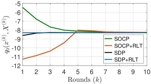
Refer to caption
Figure 2: Convergence of sequential 2×2222\times 2 SDP, 2×2222\times 2 SDP+RLT, SDP, and SDP+RLT for inst. 1507.

4.1.2 Choice of the penalty parameter η𝜂\eta

In this experiment the sensitivity of different penalization methods to the choice of the penalty parameter η𝜂\eta is tested. To this end, one round of the penalized SDP (5a)-(5d) is solved for a wide range of η𝜂\eta values. The benchmark case 1143 is used for this experiment. If η𝜂\eta is small, none of the proposed penalized SDPs are tight for the case 1143. As the value of η𝜂\eta increases, the feasibility violation tr{𝑿𝒙𝒙}tr𝑿𝒙superscript𝒙top\mathrm{tr}\{\accentset{\ast}{\boldsymbol{X}}-\accentset{\ast}{\boldsymbol{x}}\accentset{\ast}{\boldsymbol{x}}^{\top}\} abruptly vanishes once crossing η=1.9𝜂1.9\eta=1.9, η=7.7𝜂7.7\eta=7.7, and η=19.6𝜂19.6\eta=19.6, for the penalized 2×2222\times 2 SDP, SDP and SDP+RLT, respectively. Remarkably, if 𝒙SDP+RLTsuperscript𝒙SDPRLT\accentset{\ast}{\boldsymbol{x}}^{\mathrm{SDP+RLT}} is used as the initial point and η2similar-to-or-equals𝜂2\eta\simeq 2, then the penalized SDP+RLT (5a)-(5d) produces a feasible point for the benchmark case 1143 whose objective value is within 0.2% of the reported optimal cost q0(𝒙QPLIB)subscript𝑞0superscript𝒙QPLIBq_{0}(\boldsymbol{x}^{\mathrm{QPLIB}}).

Additionally, Figure 3 shows the result of one round penalized SDP for a wide range of η𝜂\eta values, on cases QPLIB 1423, 1675, and 1967. As demonstrated by the figures, the resulting objective values of penalized SDP grow slowly beyond certain limits of η𝜂\eta. This indicates that the proposed approach is not very sensitive to the choice of η𝜂\eta and a wide range of η𝜂\eta values can be used for penalization.
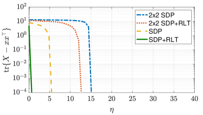
Refer to caption

​​ Refer to caption
Refer to caption​​ Refer to caption

Figure 3: The effect of η𝜂\eta on the performance of penalized 2×2222\times 2 SDP, 2×2222\times 2 SDP+RLT, SDP, and SDP+RLT for cases QPLIB 1423, 1675, and 1967.

4.2 Large-scale system identification problems

Following Fattahi and Sojoudi (2018), this case study is concerned with the problem of identifying the parameters of linear dynamical systems given limited observations and non-uniform snapshots of state vectors. Optimization is an important tool for problems involving dynamical systems such as the identification of transfer functions and control synthesis Rotkowitz and Lall (2005); Wang et al. (2019, 2018); Kheirandishfard et al. (2018b); Fattahi et al. (2018). One of these computationally-hard problems is system identification based solely on data (without intrusive means) which has been widely studied in the literature of control Sarkar and Rakhlin (2018); Pereira et al. (2010). In this case study, we cast system identification as a non-convex QCQP and evaluate the ability of the proposed penalized SDP in solving very large scale instances of this problem.

Consider a discrete-time linear system described by the system of equations:

𝒛[τ+1]𝒛delimited-[]𝜏1\displaystyle\boldsymbol{z}[\tau+1] =𝑨𝒛[τ]+𝑩𝒖[τ]+𝒘[τ]absent𝑨𝒛delimited-[]𝜏𝑩𝒖delimited-[]𝜏𝒘delimited-[]𝜏\displaystyle=\boldsymbol{A}\boldsymbol{z}[\tau]+\boldsymbol{B}\boldsymbol{u}[\tau]+\boldsymbol{w}[\tau] τ=1,2,,T1𝜏12𝑇1\displaystyle\tau=1,2,\ldots,T-1 (47a)

where

  • {𝒛[τ]n}τ=1Tsubscriptsuperscript𝒛delimited-[]𝜏superscript𝑛𝑇𝜏1\{\boldsymbol{z}[\tau]\in\mathbb{R}^{n}\}^{T}_{\tau=1} are the state vectors that are known at times τ{τ1,,τo}𝜏subscript𝜏1subscript𝜏𝑜\tau\in\{\tau_{1},\ldots,\tau_{o}\},

  • {𝒖[τ]m}τ=1Tsubscriptsuperscript𝒖delimited-[]𝜏superscript𝑚𝑇𝜏1\{\boldsymbol{u}[\tau]\in\mathbb{R}^{m}\}^{T}_{\tau=1} are the known control command vectors.

  • 𝑨n×n𝑨superscript𝑛𝑛\boldsymbol{A}\in\mathbb{R}^{n\times n} and 𝑩n×m𝑩superscript𝑛𝑚\boldsymbol{B}\in\mathbb{R}^{n\times m} are fixed unknown matrices, and

  • {𝒘[τ]n}τ=1Tsubscriptsuperscript𝒘delimited-[]𝜏superscript𝑛𝑇𝜏1\{\boldsymbol{w}[\tau]\in\mathbb{R}^{n}\}^{T}_{\tau=1} account for the unknown disturbance vectors.

Our goal is to estimate the pair of ground truth matrices (𝑨¯,𝑩¯)¯𝑨¯𝑩(\bar{\boldsymbol{A}},\bar{\boldsymbol{B}}), given a sample trajectory of the control commands {𝒖¯[τ]n}τ=1Tsubscriptsuperscript¯𝒖delimited-[]𝜏superscript𝑛𝑇𝜏1\{\bar{\boldsymbol{u}}[\tau]\in\mathbb{R}^{n}\}^{T}_{\tau=1} and the incomplete state vectors {𝒛¯[τ]n}τ{τ1,,τo}subscript¯𝒛delimited-[]𝜏superscript𝑛𝜏subscript𝜏1subscript𝜏𝑜\{\bar{\boldsymbol{z}}[\tau]\in\mathbb{R}^{n}\}_{\tau\in\{\tau_{1},\ldots,\tau_{o}\}}. To this end, we employ the minimum least absolute value estimator which amounts to the following QCQP:

minimize{𝒚[τ]n}τ=1T1{𝒛[τ]n}τ=1T𝑨n×n𝑩n×msubscriptsuperscript𝒚delimited-[]𝜏superscript𝑛𝑇1𝜏1subscriptsuperscript𝒛delimited-[]𝜏superscript𝑛𝑇𝜏1𝑨superscript𝑛𝑛𝑩superscript𝑛𝑚minimize\displaystyle\underset{\begin{subarray}{l}\phantom{\boldsymbol{B}\boldsymbol{A}\boldsymbol{z}}\{\boldsymbol{y}[\tau]\in\mathbb{R}^{n}\}^{T-1}_{\tau=1}\\ \phantom{\boldsymbol{A}\boldsymbol{B}\boldsymbol{y}}\{\boldsymbol{z}[\tau]\in\mathbb{R}^{n}\}^{T}_{\tau=1}\\ \phantom{\boldsymbol{B}\boldsymbol{y}\{\boldsymbol{z}[\tau]}\boldsymbol{A}\in\mathbb{R}^{n\times n}\\ \phantom{\boldsymbol{A}\boldsymbol{y}\{\boldsymbol{z}[\tau]}\boldsymbol{B}\in\mathbb{R}^{n\times m}\end{subarray}}{\text{minimize}} τ=1T1𝟏n𝒚[τ]subscriptsuperscript𝑇1𝜏1subscriptsuperscript1top𝑛𝒚delimited-[]𝜏\displaystyle\sum^{T-1}_{\tau=1}{\boldsymbol{1}^{\top}_{n}\boldsymbol{y}[\tau]} (48a)
   subject to 𝒚[τ]+𝒛[τ+1]𝑨𝒛[τ]𝑩𝒖¯[τ]𝒚delimited-[]𝜏𝒛delimited-[]𝜏1𝑨𝒛delimited-[]𝜏𝑩¯𝒖delimited-[]𝜏\displaystyle\boldsymbol{y}[\tau]\geq+\boldsymbol{z}[\tau+1]-\boldsymbol{A}\boldsymbol{z}[\tau]-\boldsymbol{B}\bar{\boldsymbol{u}}[\tau] τ{1,2,,T1},𝜏12𝑇1\displaystyle\tau\in\{1,2,\ldots,T-1\}, (48b)
𝒚[τ]𝒛[τ+1]+𝑨𝒛[τ]+𝑩𝒖¯[τ]𝒚delimited-[]𝜏𝒛delimited-[]𝜏1𝑨𝒛delimited-[]𝜏𝑩¯𝒖delimited-[]𝜏\displaystyle\boldsymbol{y}[\tau]\geq-\boldsymbol{z}[\tau+1]+\boldsymbol{A}\boldsymbol{z}[\tau]+\boldsymbol{B}\bar{\boldsymbol{u}}[\tau] τ{1,2,,T1},𝜏12𝑇1\displaystyle\tau\in\{1,2,\ldots,T-1\}, (48c)
𝒛[τ]=𝒛¯[τ]𝒛delimited-[]𝜏¯𝒛delimited-[]𝜏\displaystyle\boldsymbol{z}[\tau]=\bar{\boldsymbol{z}}[\tau] τ{τ1,,τo}.𝜏subscript𝜏1subscript𝜏𝑜\displaystyle\tau\in\{\tau_{1},\ldots,\tau_{o}\}. (48d)

For every τ{1,2,,T1}𝜏12𝑇1\tau\in\{1,2,\ldots,T-1\}, the auxiliary variable 𝒚[τ]n𝒚delimited-[]𝜏superscript𝑛\boldsymbol{y}[\tau]\in\mathbb{R}^{n} accounts for |𝒛[τ+1]𝑨𝒛[τ]𝑩𝒖¯[τ]|𝒛delimited-[]𝜏1𝑨𝒛delimited-[]𝜏𝑩¯𝒖delimited-[]𝜏|\boldsymbol{z}[\tau+1]-\boldsymbol{A}\boldsymbol{z}[\tau]-\boldsymbol{B}\bar{\boldsymbol{u}}[\tau]|. This relation is imposed through the pair of constraints (48b) and (48c).

The problem (48a)–(48d), can be cast in the form of (1a)-(1c), with respect to the vector

𝒙[𝒛[1],,𝒛[T],vec{𝑨},α𝒚[1],,α𝒚[T1],αvec{𝑩}],𝒙𝒛superscriptdelimited-[]1top𝒛superscriptdelimited-[]𝑇topvecsuperscript𝑨top𝛼𝒚superscriptdelimited-[]1top𝛼𝒚superscriptdelimited-[]𝑇1top𝛼vecsuperscript𝑩top\displaystyle\boldsymbol{x}\triangleq[\boldsymbol{z}[1]^{\top},\,\ldots,\,\boldsymbol{z}[T]^{\top},\mathrm{vec}\{\boldsymbol{A}\}^{\top},\alpha\,\boldsymbol{y}[1]^{\top},\,\ldots,\,\alpha\,\boldsymbol{y}[T-1]^{\top},\alpha\,\mathrm{vec}\{\boldsymbol{B}\}^{\top}],\!\!\! (49)

where α𝛼\alpha is a preconditioning constant. To solve the resulting problem, we use the sequential Algorithm 1 equipped with the 2×2222\times 2 SDP relaxation and the initial point 𝒙^=𝟎^𝒙0\hat{\boldsymbol{x}}=\boldsymbol{0}.

We consider system identification problems with n=25𝑛25n=25, m=20𝑚20m=20, T=500𝑇500T=500 and o=400𝑜400o=400. In every experiment, {τ1,,τo}subscript𝜏1subscript𝜏𝑜\{\tau_{1},\ldots,\tau_{o}\} is a uniformly selected subset of {1,2,,T}12𝑇\{1,2,\ldots,T\}. The resulting QCQP variable 𝒙𝒙\boldsymbol{x} is 236052360523605-dimensional and the problem is 161001610016100-dimensional if we exclude the known state vectors {𝒛¯[τ]n}τ{τ1,,τo}subscript¯𝒛delimited-[]𝜏superscript𝑛𝜏subscript𝜏1subscript𝜏𝑜\{\bar{\boldsymbol{z}}[\tau]\in\mathbb{R}^{n}\}_{\tau\in\{\tau_{1},\ldots,\tau_{o}\}}. Due to sparsity of the QCQP (48a)-(48d) each round of the penalized 2×2222\times 2 SDP is solved within 30 minutes, by omitting the elements of the lifted variable 𝑿𝑿\boldsymbol{X} that do not appear in the objective and constraints. All of the convex programs are solved using MOSEK v8.1 ApS (2017) through MATLAB 2017a and on a desktop computer with a 12-core 3.0GHz CPU and 256GB RAM. Due to the sheer size of this problem, we were only able to solve instances with T70𝑇70T\leq 70 using BARON and COUENNE non of which resulted in successful recovery of the unknown matrices due to limited data points.
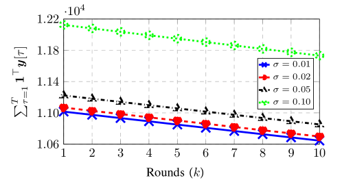
Refer to caption
Figure 4: Convergence of the sequential penalized 2×2222\times 2 SDP for large-scale system identification with different disturbance levels.

The ground truth values are chosen as follows:

  • The elements of 𝑨¯25×25¯𝑨superscript2525\bar{\boldsymbol{A}}\in\mathbb{R}^{25\times 25} have zero-mean Gaussian distribution and the matrix is scaled in such a way that the largest singular value is equal to 0.50.50.5.

  • Every element of 𝑩¯25×20¯𝑩superscript2520\bar{\boldsymbol{B}}\in\mathbb{R}^{25\times 20}, {𝒖¯[τ]20}τ=1Tsubscriptsuperscript¯𝒖delimited-[]𝜏superscript20𝑇𝜏1\{\bar{\boldsymbol{u}}[\tau]\in\mathbb{R}^{20}\}^{T}_{\tau=1} and 𝒛¯[1]25¯𝒛delimited-[]1superscript25\bar{\boldsymbol{z}}[1]\in\mathbb{R}^{25} have standard normal distribution.

  • The elements of {𝒘¯[τ]25}τ=1T1subscriptsuperscript¯𝒘delimited-[]𝜏superscript25𝑇1𝜏1\{\bar{\boldsymbol{w}}[\tau]\in\mathbb{R}^{25}\}^{T-1}_{\tau=1} have independent zero-mean Gaussian distribution with the standard deviation σ{0.01,0.02,0.05,0.10}𝜎0.010.020.050.10\sigma\in\{0.01,0.02,0.05,0.10\}.

For each experiment, we ran Algorithm 1 for 10 rounds. The preconditioning and penalty terms are set to α=103𝛼superscript103\alpha=10^{-3} and η=40𝜂40\eta=40, respectively. For each σ{0.01,0.02,\sigma\in\{0.01,0.02, 0.05,0.10}0.05,0.10\}, we have run 10 random experiments resulting in the average recovery errors 0.00050.00050.0005, 0.00100.00100.0010, 0.00260.00260.0026, and 0.00620.00620.0062, respectively, for 1n𝑨¯𝑨(10)F1𝑛subscriptnorm¯𝑨superscript𝑨10𝐹\frac{1}{n}\|\bar{\boldsymbol{A}}-\boldsymbol{A}^{(10)}\|_{F}, and the average errors 0.00140.00140.0014, 0.00280.00280.0028, 0.00700.00700.0070, and 0.01410.01410.0141, respectively, for (mn)12𝑩¯𝑩(10)Fsuperscript𝑚𝑛12subscriptnorm¯𝑩superscript𝑩10𝐹(mn)^{-\frac{1}{2}}\|\bar{\boldsymbol{B}}-\boldsymbol{B}^{(10)}\|_{F}. In all of the trials, a feasible point is obtained in the first round of Algorithm 1. Figure 4 illustrates the convergence behavior of the objective functions for one of the trials for each disturbance level.

5 Conclusions

This paper introduces a penalization approach for constructing feasible and near-optimal solutions to non-convex quadratically-constrained quadratic programming (QCQP) problems. Given an arbitrary initial point (feasible or infeasible) for the original QCQP, penalized semidefinite programs are formulated by adding a linear term to the objective. A generalized linear independence constraint qualification (LICQ) condition is introduced as a regularity criterion for initial points, and it is shown that the solution of penalized SDP is feasible for QCQP if the initial point is regular and close to the feasible set. We show that the proposed penalized SDPs can be solved sequentially in order to improve the objective of the feasible solution. Numerical experiments on QPLIB benchmark cases demonstrate that the proposed sequential approach compares favorably with non-convex optimizers BARON and COUENNE. Moreover, the scalability of the proposed method is demonstrated on large-scale system identification problems.

Acknowledgements.
The authors are grateful to GAMS Development Corporation for providing them with unrestricted access to a full set of solvers throughout the project.

References

  • Ahmadi and Majumdar (2019) Ahmadi AA, Majumdar A (2019) DSOS and SDSOS optimization: more tractable alternatives to sum of squares and semidefinite optimization. SIAM Journal on Applied Algebraic Geometry 3(2):193–230
  • Aittomaki and Koivunen (2009) Aittomaki T, Koivunen V (2009) Beam pattern optimization by minimization of quartic polynomial. In: 2009 IEEE/SP 15th Workshop on Statistical Signal Processing, IEEE, pp 437–440
  • Alizadeh and Goldfarb (2003) Alizadeh F, Goldfarb D (2003) Second-order cone programming. Mathematical Programming 95(1):3–51
  • ApS (2017) ApS M (2017) The MOSEK optimization toolbox for MATLAB manual. Version 8.1. URL http://docs.mosek.com/8.1/toolbox/index.html
  • Ashraphijuo et al. (2016) Ashraphijuo M, Madani R, Lavaei J (2016) Characterization of rank-constrained feasibility problems via a finite number of convex programs. In: 2016 IEEE 55th Conference on Decision and Control (CDC), IEEE, pp 6544–6550
  • Atamtürk and Gómez (2019) Atamtürk A, Gómez A (2019) Rank-one convexification for sparse regression. arXiv preprint arXiv:190110334
  • Atamtürk and Narayanan (2007) Atamtürk A, Narayanan V (2007) Cuts for conic mixed-integer programming. In: Fischetti M, Williamson DP (eds) Integer Programming and Combinatorial Optimization, Springer, Berlin, Heidelberg, pp 16–29
  • Aubry et al. (2013) Aubry A, De Maio A, Jiang B, Zhang S (2013) Ambiguity function shaping for cognitive radar via complex quartic optimization. IEEE Transactions on Signal Processing 61(22):5603–5619
  • Bandeira et al. (2014) Bandeira AS, Boumal N, Singer A (2014) Tightness of the maximum likelihood semidefinite relaxation for angular synchronization. arXiv preprint arXiv:14113272
  • Bao et al. (2011) Bao X, Sahinidis NV, Tawarmalani M (2011) Semidefinite relaxations for quadratically constrained quadratic programming: A review and comparisons. Mathematical Programming 129:129–157
  • Belotti (2013) Belotti P (2013) COUENNE: A user’s manual. Tech. rep., Technical report, Lehigh University
  • Bienstock and Munoz (2018) Bienstock D, Munoz G (2018) LP formulations for polynomial optimization problems. SIAM Journal on Optimization 28(2):1121–1150
  • Burer and Vandenbussche (2008) Burer S, Vandenbussche D (2008) A finite branch-and-bound algorithm for nonconvex quadratic programming via semidefinite relaxations. Mathematical Programming 113(2):259–282
  • Burer and Ye (2018) Burer S, Ye Y (2018) Exact semidefinite formulations for a class of (random and non-random) nonconvex quadratic programs. arXiv preprint arXiv:180202688
  • Burgdorf et al. (2015) Burgdorf S, Laurent M, Piovesan T (2015) On the closure of the completely positive semidefinite cone and linear approximations to quantum colorings. arXiv preprint arXiv:150202842
  • Candès and Recht (2009) Candès EJ, Recht B (2009) Exact matrix completion via convex optimization. Foundations of Computational Mathematics 9(6):717–772
  • Candes et al. (2013) Candes EJ, Strohmer T, Voroninski V (2013) Phaselift: Exact and stable signal recovery from magnitude measurements via convex programming. Communications on Pure and Applied Mathematics 66(8):1241–1274
  • Candes et al. (2015) Candes EJ, Eldar YC, Strohmer T, Voroninski V (2015) Phase retrieval via matrix completion. SIAM Review 57(2):225–251
  • Chen et al. (2017) Chen C, Atamtürk A, Oren SS (2017) A spatial branch-and-cut method for nonconvex QCQP with bounded complex variables. Mathematical Programming 165(2):549–577
  • Chen and Vaidyanathan (2009) Chen CY, Vaidyanathan P (2009) Mimo radar waveform optimization with prior information of the extended target and clutter. IEEE Transactions on Signal Processing 57(9):3533–3544
  • Chen and Burer (2012) Chen J, Burer S (2012) Globally solving nonconvex quadratic programming problems via completely positive programming. Mathematical Programming Computation 4(1):33–52
  • Cid et al. (2004) Cid C, Murphy S, Robshaw M (2004) Computational and algebraic aspects of the advanced encryption standard. In: Proceedings of the Seventh International Workshop on Computer Algebra in Scientific Computing-CASC, vol 2004
  • Cid et al. (2005) Cid C, Murphy S, Robshaw MJ (2005) Small scale variants of the aes. In: International Workshop on Fast Software Encryption, Springer, pp 145–162
  • Courtois and Pieprzyk (2002) Courtois NT, Pieprzyk J (2002) Cryptanalysis of block ciphers with overdefined systems of equations. In: International Conference on the Theory and Application of Cryptology and Information Security, Springer, pp 267–287
  • Deza and Laurent (1994) Deza M, Laurent M (1994) Applications of cut polyhedra-II. Journal of Computational and Applied Mathematics 55(2):217–247
  • Fattahi and Sojoudi (2018) Fattahi S, Sojoudi S (2018) Data-driven sparse system identification. In: 56th Annual Allerton Conference on Communication, Control, and Computing (Allerton), IEEE
  • Fattahi et al. (2018) Fattahi S, Fazelnia G, Lavaei J, Arcak M (2018) Transformation of optimal centralized controllers into near-globally optimal static distributed controllers. IEEE Transactions on Automatic Control 64(1):66–80
  • Fazelnia et al. (2017) Fazelnia G, Madani R, Kalbat A, Lavaei J (2017) Convex relaxation for optimal distributed control problems. IEEE Transactions on Automatic Control 62(1):206–221
  • Fogel et al. (2016) Fogel F, Waldspurger I, dAspremont A (2016) Phase retrieval for imaging problems. Mathematical Programming Computation 8:311–335
  • Furini et al. (2019) Furini F, Traversi E, Belotti P, Frangioni A, Gleixner A, Gould N, Liberti L, Lodi A, Misener R, Mittelmann H, Sahinidis N, Vigerske S, Wiegele A (2019) QPLIB: A library of quadratic programming instances. Mathematical Programming Computation 11:237–310, URL http://qplib.zib.de/
  • GAMS Development Corporation (2013) GAMS Development Corporation (2013) General Algebraic Modeling System (GAMS) Release 24.2.1. Washington, DC, USA, URL http://www.gams.com/
  • Gershman et al. (2010) Gershman AB, Sidiropoulos ND, Shahbazpanahi S, Bengtsson M, Ottersten B (2010) Convex optimization-based beamforming: From receive to transmit and network designs. IEEE Signal Process Mag 27(3):62–75
  • Goemans and Williamson (1995) Goemans MX, Williamson DP (1995) Improved approximation algorithms for maximum cut and satisfiability problems using semidefinite programming. Journal of the ACM (JACM) 42(6):1115–1145
  • Han et al. (2020) Han S, Gómez A, Atamtürk A (2020) 2x2-convexifications for convex quadratic optimization with indicator variables. arXiv preprint arXiv:200407448
  • He et al. (2008) He S, Luo Z, Nie J, Zhang S (2008) Semidefinite relaxation bounds for indefinite homogeneous quadratic optimization. SIAM Journal on Optimization 19:503–523
  • He et al. (2010) He S, Li Z, Zhang S (2010) Approximation algorithms for homogeneous polynomial optimization with quadratic constraints. Mathematical Programming 125:353–383
  • Hilling and Sudbery (2010) Hilling JJ, Sudbery A (2010) The geometric measure of multipartite entanglement and the singular values of a hypermatrix. Journal of Mathematical Physics 51(7):072102
  • Ibaraki and Tomizuka (2001) Ibaraki S, Tomizuka M (2001) Rank minimization approach for solving BMI problems with random search. In: Proceedings of the 2001 American Control Conference.(Cat. No. 01CH37148), IEEE, vol 3, pp 1870–1875
  • Josz and Molzahn (2018) Josz C, Molzahn DK (2018) Lasserre hierarchy for large scale polynomial optimization in real and complex variables. SIAM Journal on Optimization 28(2):1017–1048
  • Kheirandishfard et al. (2018a) Kheirandishfard M, Zohrizadeh F, Adil M, Madani R (2018a) Convex relaxation of bilinear matrix inequalities part II: Applications to optimal control synthesis. In: IEEE 57th Annual Conference on Decision and Control (CDC)
  • Kheirandishfard et al. (2018b) Kheirandishfard M, Zohrizadeh F, Adil M, Madani R (2018b) Convex relaxation of bilinear matrix inequalities part ii: Applications to optimal control synthesis. In: 2018 IEEE Conference on Decision and Control (CDC), IEEE, pp 75–82
  • Kheirandishfard et al. (2018c) Kheirandishfard M, Zohrizadeh F, Madani R (2018c) Convex relaxation of bilinear matrix inequalities part I: Theoretical results. In: IEEE 57th Annual Conference on Decision and Control (CDC),
  • Kim and Kojima (2003) Kim S, Kojima M (2003) Exact solutions of some nonconvex quadratic optimization problems via SDP and SOCP relaxations. Computational Optimization and Applications 26(2):143–154
  • Kim et al. (2003) Kim S, Kojima M, Yamashita M (2003) Second order cone programming relaxation of a positive semidefinite constraint. Optimization Methods and Software 18:535–541
  • Lasserre (2001a) Lasserre JB (2001a) An explicit exact SDP relaxation for nonlinear 0-1 programs. In: Integer Programming and Combinatorial Optimization, Springer, pp 293–303
  • Lasserre (2001b) Lasserre JB (2001b) Global optimization with polynomials and the problem of moments. SIAM Journal on Optimization 11:796–817
  • Lasserre (2006) Lasserre JB (2006) Convergent SDP-relaxations in polynomial optimization with sparsity. SIAM Journal on Optimization 17:822–843
  • Laurent and Piovesan (2015) Laurent M, Piovesan T (2015) Conic approach to quantum graph parameters using linear optimization over the completely positive semidefinite cone. SIAM Journal on Optimization 25(4):2461–2493
  • Li et al. (2012) Li Z, He S, Zhang S (2012) Approximation methods for polynomial optimization: Models, Algorithms, and Applications. Springer Science & Business Media
  • Lovász and Schrijver (1991) Lovász L, Schrijver A (1991) Cones of matrices and set-functions and 0–1 optimization. SIAM Journal on Optimization 1(2):166–190
  • Luo et al. (2007) Luo Z, Sidiropoulos N, Tseng P, Zhang S (2007) Approximation bounds for quadratic optimization with homogeneous quadratic constraints. SIAM Journal on Optimization 18:1–28
  • Luo et al. (2010) Luo ZQ, Ma Wk, So AMC, Ye Y, Zhang S (2010) Semidefinite relaxation of quadratic optimization problems. IEEE Signal Processing Magazine 27(3):20–34
  • Madani et al. (2014) Madani R, Fazelnia G, Lavaei J (2014) Rank-2 matrix solution for semidefinite relaxations of arbitrary polynomial optimization problems. Preprint
  • Madani et al. (2015a) Madani R, Lavaei J, Baldick R (2015a) Convexification of power flow problem over arbitrary networks. In: 2015 54th IEEE Conference on Decision and Control (CDC), IEEE, pp 1–8
  • Madani et al. (2015b) Madani R, Sojoudi S, Lavaei J (2015b) Convex relaxation for optimal power flow problem: Mesh networks. IEEE Transactions on Power Systems 30(1):199–211
  • Madani et al. (2016) Madani R, Ashraphijuo M, Lavaei J (2016) Promises of conic relaxation for contingency-constrained optimal power flow problem. IEEE Transactions on Power Systems 31(2):1297–1307
  • Madani et al. (2017a) Madani R, Atamtürk A, Davoudi A (2017a) A scalable semidefinite relaxation approach to grid scheduling. arXiv preprint arXiv:170703541
  • Madani et al. (2017b) Madani R, Sojoudi S, Fazelnia G, Lavaei J (2017b) Finding low-rank solutions of sparse linear matrix inequalities using convex optimization. SIAM Journal on Optimization 27(2):725–758
  • Majumdar et al. (2014) Majumdar A, Ahmadi AA, Tedrake R (2014) Control and verification of high-dimensional systems with DSOS and SDSOS programming. In: Decision and Control (CDC), 2014 IEEE 53rd Annual Conference on, IEEE, pp 394–401
  • Mariere et al. (2003) Mariere B, Luo ZQ, Davidson TN (2003) Blind constant modulus equalization via convex optimization. IEEE Transactions on Signal Processing 51(3):805–818
  • Mohammad-Nezhad and Terlaky (2017) Mohammad-Nezhad A, Terlaky T (2017) A rounding procedure for semidefinite optimization. Submitted to Operations Research Letters
  • Mu et al. (2016) Mu C, Zhang Y, Wright J, Goldfarb D (2016) Scalable robust matrix recovery: Frank–Wolfe meets proximal methods. SIAM Journal on Scientific Computing 38(5):A3291–A3317
  • Muramatsu and Suzuki (2003) Muramatsu M, Suzuki T (2003) A new second-order cone programming relaxation for max-cut problems. Journal of the Operations Research Society of Japan 46:164–177
  • Murphy and Robshaw (2002) Murphy S, Robshaw MJ (2002) Essential algebraic structure within the aes. In: Annual International Cryptology Conference, Springer, pp 1–16
  • Natarajan et al. (2013) Natarajan K, Shi D, Toh KC (2013) A penalized quadratic convex reformulation method for random quadratic unconstrained binary optimization. Optimization Online
  • Nesterov (1998) Nesterov Y (1998) Semidefinite relaxation and nonconvex quadratic optimization. Optimization Methods and Software 9:141–160
  • Nesterov et al. (1994) Nesterov Y, Nemirovskii AS, Ye Y (1994) Interior-point polynomial algorithms in convex programming. SIAM
  • Papp and Alizadeh (2013) Papp D, Alizadeh F (2013) Semidefinite characterization of sum-of-squares cones in algebras. SIAM Journal on Optimization 23(3):1398–1423
  • Pereira et al. (2010) Pereira J, Ibrahimi M, Montanari A (2010) Learning networks of stochastic differential equations. In: Advances in Neural Information Processing Systems, pp 172–180
  • Permenter and Parrilo (2018) Permenter F, Parrilo P (2018) Partial facial reduction: simplified, equivalent SDPs via approximations of the PSD cone. Mathematical Programming 171:1–54
  • Rotkowitz and Lall (2005) Rotkowitz M, Lall S (2005) A characterization of convex problems in decentralized control. IEEE transactions on Automatic Control 50(12):1984–1996
  • Sarkar and Rakhlin (2018) Sarkar T, Rakhlin A (2018) How fast can linear dynamical systems be learned? arXiv preprint arXiv:181201251
  • Sherali and Adams (1990) Sherali HD, Adams WP (1990) A hierarchy of relaxations between the continuous and convex hull representations for zero-one programming problems. SIAM Journal on Discrete Mathematics 3(3):411–430
  • Sherali and Adams (2013) Sherali HD, Adams WP (2013) A reformulation-linearization technique for solving discrete and continuous nonconvex problems, vol 31. Springer Science & Business Media
  • Singer (2011) Singer A (2011) Angular synchronization by eigenvectors and semidefinite programming. Applied and Computational Harmonic Analysis 30(1):20–36
  • Sojoudi and Lavaei (2013a) Sojoudi S, Lavaei J (2013a) On the exactness of semidefinite relaxation for nonlinear optimization over graphs: Part I. In: Decision and Control (CDC), 2013 IEEE 52nd Annual Conference on, IEEE, pp 1043–1050
  • Sojoudi and Lavaei (2013b) Sojoudi S, Lavaei J (2013b) On the exactness of semidefinite relaxation for nonlinear optimization over graphs: Part II. In: Decision and Control (CDC), 2013 IEEE 52nd Annual Conference on, IEEE, pp 1043–1050
  • Tawarmalani and Sahinidis (2005) Tawarmalani M, Sahinidis NV (2005) A polyhedral branch-and-cut approach to global optimization. Mathematical Programming 103:225–249
  • Toker and Ozbay (1998) Toker O, Ozbay H (1998) On the complexity of purely complex μ𝜇\mu computation and related problems in multidimensional systems. IEEE Transactions on Automatic Control 43(3):409–414
  • Wang et al. (2018) Wang YS, Matni N, Doyle JC (2018) Separable and localized system-level synthesis for large-scale systems. IEEE Transactions on Automatic Control 63(12):4234–4249
  • Wang et al. (2019) Wang YS, Matni N, Doyle JC (2019) A system level approach to controller synthesis. IEEE Transactions on Automatic Control
  • Ye (1999a) Ye Y (1999a) Approximating global quadratic optimization with convex quadratic constraints. Journal of Global Optimization 15:1–17
  • Ye (1999b) Ye Y (1999b) Approximating quadratic programming with bound and quadratic constraints. Mathematical Programming 84:219–226
  • Zhang (2000) Zhang S (2000) Quadratic maximization and semidefinite relaxation. Mathematical Programming 87:453–465
  • Zhang and Huang (2006) Zhang S, Huang Y (2006) Complex quadratic optimization and semidefinite programming. SIAM Journal on Optimization 87:871–890
  • Zohrizadeh et al. (2018a) Zohrizadeh F, Kheirandishfard M, Nasir A, Madani R (2018a) Sequential relaxation of unit commitment with AC transmission constraints. In: IEEE 57th Annual Conference on Decision and Control (CDC)
  • Zohrizadeh et al. (2018b) Zohrizadeh F, Kheirandishfard M, Quarm E, Madani R (2018b) Penalized parabolic relaxation for optimal power flow problem. In: IEEE 57th Annual Conference on Decision and Control (CDC)

Appendix A Application to polynomial optimization

In this section, we show that the proposed penalized SDP approach can be used for polynomial optimization as well. A polynomial optimization problem is formulated as

minimize𝒙n𝒙superscript𝑛minimize\displaystyle\underset{\boldsymbol{x}\in\mathbb{R}^{n}}{\text{minimize}}\ \ u0(𝒙)subscript𝑢0𝒙\displaystyle u_{0}(\boldsymbol{x}) (50a)
s.t. uk(𝒙)0,kformulae-sequencesubscript𝑢𝑘𝒙0𝑘\displaystyle u_{k}(\boldsymbol{x})\leq 0,\quad\quad k\in\mathcal{I} (50b)
uk(𝒙)=0,k,formulae-sequencesubscript𝑢𝑘𝒙0𝑘\displaystyle u_{k}(\boldsymbol{x})=0,\quad\quad k\in\mathcal{E}, (50c)

for every k{0}𝑘0k\in\{0\}\cup\mathcal{I}\cup\mathcal{E}, where each function uk:n:subscript𝑢𝑘superscript𝑛u_{k}:\mathbb{R}^{n}\to\mathbb{R} is a polynomial of arbitrary degree. Problem (50a)–(50c) can be reformulated as a QCQP of the form:

minimize𝒙n,𝒚oformulae-sequence𝒙superscript𝑛𝒚superscript𝑜minimize\displaystyle\underset{\begin{subarray}{l}\boldsymbol{x}\in\mathbb{R}^{n},{\boldsymbol{y}}\in\mathbb{R}^{o}\end{subarray}}{\!\!\text{minimize}}\ \ w0(𝒙,𝒚)subscript𝑤0𝒙𝒚\displaystyle\!\!\!\!\phantom{v_{i}}w_{0}(\boldsymbol{x},\boldsymbol{y}) (51a)
s.t. wk(𝒙,𝒚)0,kformulae-sequencesubscript𝑤𝑘𝒙𝒚0𝑘\displaystyle\!\!\!\!\phantom{v_{i}}w_{k}(\boldsymbol{x},\boldsymbol{y})\leq 0,\quad\quad k\in\mathcal{I} (51b)
wk(𝒙,𝒚)=0,kformulae-sequencesubscript𝑤𝑘𝒙𝒚0𝑘\displaystyle\!\!\!\!\phantom{v_{i}}w_{k}(\boldsymbol{x},\boldsymbol{y})=0,\quad\quad k\in\mathcal{E} (51c)
vi(𝒙,𝒚)=0,i𝒪,formulae-sequencesubscript𝑣𝑖𝒙𝒚0𝑖𝒪\displaystyle\!\!\!\!\phantom{w_{k}}v_{i}(\boldsymbol{x},\boldsymbol{y})=0,\quad\quad i\in\mathcal{O}, (51d)

where 𝒚|𝒪|𝒚superscript𝒪\boldsymbol{y}\in\mathbb{R}^{|\mathcal{O}|} is an auxiliary variable, and v1,,v|𝒪|subscript𝑣1subscript𝑣𝒪v_{1},\ldots,v_{|\mathcal{O}|} and w0,w1,,w|{0}|subscript𝑤0subscript𝑤1subscript𝑤0w_{0},w_{1},\ldots,w_{|\{0\}\cup\mathcal{I}\cup\mathcal{E}|} are quadratic functions with the following properties:

  • For every 𝒙n𝒙superscript𝑛\boldsymbol{x}\in\mathbb{R}^{n}, the function 𝒗(𝒙,):|𝒪||𝒪|:𝒗𝒙superscript𝒪superscript𝒪\boldsymbol{v}(\boldsymbol{x},\cdot):\mathbb{R}^{|\mathcal{O}|}\to\mathbb{R}^{|\mathcal{O}|} is invertible,

  • If 𝒗(𝒙,𝒚)=𝟎n𝒗𝒙𝒚subscript0𝑛\boldsymbol{v}(\boldsymbol{x},\boldsymbol{y})=\boldsymbol{0}_{n}, then wk(𝒙,𝒚)=uk(𝒙)subscript𝑤𝑘𝒙𝒚subscript𝑢𝑘𝒙w_{k}(\boldsymbol{x},\boldsymbol{y})=u_{k}(\boldsymbol{x}) for every k{0}𝑘0k\in\{0\}\cup\mathcal{I}\cup\mathcal{E}.

Based on the above properties, there is a one-to-one correspondence between the feasible sets of (50a)–(50c) and (51a)–(51d). Moreover, a feasible point (𝒙,𝒚)𝒙𝒚(\accentset{\ast}{\boldsymbol{x}},\accentset{\ast}{\boldsymbol{y}}) is an optimal solution to the QCQP (51a)–(51d) if and only if 𝒙𝒙\accentset{\ast}{\boldsymbol{x}} is an optimal solution to the polynomial optimization problem (50a)–(50c).

Theorem A.1 (​​Madani et al. (2014))

Suppose that {uk}k{0}subscriptsubscript𝑢𝑘𝑘0\{u_{k}\}_{k\in\{0\}\cup\mathcal{I}\cup\mathcal{E}} are polynomials of degree at most d𝑑d, consisting of m𝑚m monomials in total. There exists a QCQP reformulation of the polynomial optimization (50a)–(50c) in the form of (51a)–(51d), where |𝒪|mn(log2(d)+1)𝒪𝑚𝑛subscript2𝑑1{|\mathcal{O}|}\leq mn\left(\lfloor\log_{2}(d)\rfloor+1\right).

The next proposition shows that the LICQ regularity of a point 𝒙^n^𝒙superscript𝑛\hat{\boldsymbol{x}}\in\mathbb{R}^{n} is inherited by the corresponding point (𝒙^,𝒚^)n×o^𝒙^𝒚superscript𝑛superscript𝑜(\hat{\boldsymbol{x}},\hat{\boldsymbol{y}})\in\mathbb{R}^{n}\times\mathbb{R}^{o} of the QCQP reformulation (51a)-(51d).

Proposition 1

Consider a pair of vectors 𝐱^n^𝐱superscript𝑛\hat{\boldsymbol{x}}\in\mathbb{R}^{n} and 𝐲^|𝒪|^𝐲superscript𝒪\hat{\boldsymbol{y}}\in\mathbb{R}^{|\mathcal{O}|} satisfying 𝐯(𝐱^,𝐲^)=𝟎n𝐯^𝐱^𝐲subscript0𝑛\boldsymbol{v}(\hat{\boldsymbol{x}},\hat{\boldsymbol{y}})=\boldsymbol{0}_{n}. The following two statements are equivalent:

  1. 1.

    𝒙^^𝒙\hat{\boldsymbol{x}} is feasible and satisfies the LICQ condition for the polynomial optimization problem (50a)–(50b).

  2. 2.

    (𝒙^,𝒚^)^𝒙^𝒚(\hat{\boldsymbol{x}},\hat{\boldsymbol{y}}) is feasible and satisfies the LICQ condition for the QCQP (51a)–(51d).

Proof

From 𝒖(𝒙^)=𝒘(𝒙^,𝒚^)𝒖^𝒙𝒘^𝒙^𝒚\boldsymbol{u}(\hat{\boldsymbol{x}})=\boldsymbol{w}(\hat{\boldsymbol{x}},\hat{\boldsymbol{y}}) and the invertiblity assumption for 𝒗(𝒙^,)𝒗^𝒙\boldsymbol{v}(\hat{\boldsymbol{x}},\cdot), we have

𝒖(𝒙^)𝒙𝒖^𝒙𝒙\displaystyle\!\!\!\!\!\frac{\partial\boldsymbol{u}(\hat{\boldsymbol{x}})}{\partial\boldsymbol{x}} =[𝒘(𝒙^,𝒚^)𝒙𝒘(𝒙^,𝒚^)𝒚][𝑰(𝒗(𝒙^,𝒚^)𝒚)1𝒗(𝒙^,𝒚^)𝒙]absentmatrix𝒘^𝒙^𝒚𝒙𝒘^𝒙^𝒚𝒚superscriptmatrix𝑰superscript𝒗^𝒙^𝒚𝒚1𝒗^𝒙^𝒚𝒙top\displaystyle\!=\!\!\begin{bmatrix}\frac{\partial\boldsymbol{w}(\hat{\boldsymbol{x}},\hat{\boldsymbol{y}})}{\partial\boldsymbol{x}}&\frac{\partial\boldsymbol{w}(\hat{\boldsymbol{x}},\hat{\boldsymbol{y}})}{\partial\boldsymbol{y}}\end{bmatrix}\!\!\begin{bmatrix}\boldsymbol{I}&-\!\left(\!\frac{\partial\boldsymbol{v}(\hat{\boldsymbol{x}},\hat{\boldsymbol{y}})}{\partial\boldsymbol{y}}\!\right)^{\!\!-1}\frac{\partial\boldsymbol{v}(\hat{\boldsymbol{x}},\hat{\boldsymbol{y}})}{\partial\boldsymbol{x}}\!\end{bmatrix}^{\!\top}
=𝒘(𝒙^,𝒚^)𝒙𝒘(𝒙^,𝒚^)𝒚(𝒗(𝒙^,𝒚^)𝒚)1𝒗(𝒙^,𝒚^)𝒙.absent𝒘^𝒙^𝒚𝒙𝒘^𝒙^𝒚𝒚superscript𝒗^𝒙^𝒚𝒚1𝒗^𝒙^𝒚𝒙\displaystyle=\!\frac{\partial\boldsymbol{w}(\hat{\boldsymbol{x}},\hat{\boldsymbol{y}})}{\partial\boldsymbol{x}}\!-\!\frac{\partial\boldsymbol{w}(\hat{\boldsymbol{x}},\hat{\boldsymbol{y}})}{\partial\boldsymbol{y}}\!\left(\!\frac{\partial\boldsymbol{v}(\hat{\boldsymbol{x}},\hat{\boldsymbol{y}})}{\partial\boldsymbol{y}}\!\right)^{\!\!-1}\!\frac{\partial\boldsymbol{v}(\hat{\boldsymbol{x}},\hat{\boldsymbol{y}})}{\partial\boldsymbol{x}}.\!\!\! (52)

Therefore, 𝒥PO(𝒙^)=𝒖(𝒙^)𝒙subscript𝒥PO^𝒙𝒖^𝒙𝒙\mathcal{J}_{\mathrm{PO}}(\hat{\boldsymbol{x}})=\frac{\partial\boldsymbol{u}(\hat{\boldsymbol{x}})}{\partial\boldsymbol{x}} is equal to the Schur complement of

𝒥QCQP(𝒙^,𝒚^)=[𝒘(𝒙^,𝒚^)𝒙𝒘(𝒙^,𝒚^)𝒚𝒗(𝒙^,𝒚^)𝒙𝒗(𝒙^,𝒚^)𝒚],subscript𝒥QCQP^𝒙^𝒚matrix𝒘^𝒙^𝒚𝒙𝒘^𝒙^𝒚𝒚𝒗^𝒙^𝒚𝒙𝒗^𝒙^𝒚𝒚\displaystyle\mathcal{J}_{\mathrm{QCQP}}(\hat{\boldsymbol{x}},\hat{\boldsymbol{y}})=\begin{bmatrix}\frac{\partial\boldsymbol{w}(\hat{\boldsymbol{x}},\hat{\boldsymbol{y}})}{\partial\boldsymbol{x}}&\frac{\partial\boldsymbol{w}(\hat{\boldsymbol{x}},\hat{\boldsymbol{y}})}{\partial\boldsymbol{y}}\\ \frac{\partial\boldsymbol{v}(\hat{\boldsymbol{x}},\hat{\boldsymbol{y}})}{\partial\boldsymbol{x}}&\frac{\partial\boldsymbol{v}(\hat{\boldsymbol{x}},\hat{\boldsymbol{y}})}{\partial\boldsymbol{y}}\\ \end{bmatrix}, (53)

which is the Jacobian matrix of the QCQP (51a)–(51d) at the point (𝒙^,𝒚^)^𝒙^𝒚(\hat{\boldsymbol{x}},\hat{\boldsymbol{y}}). As a result, the matrix 𝒥PO(𝒙^)subscript𝒥PO^𝒙\mathcal{J}_{\mathrm{PO}}(\hat{\boldsymbol{x}}) is singular if and only if 𝒥QCQP(𝒙^,𝒚^)subscript𝒥QCQP^𝒙^𝒚\mathcal{J}_{\mathrm{QCQP}}(\hat{\boldsymbol{x}},\hat{\boldsymbol{y}}) is singular.

Appendix B Reformulation-Linearization Technique

This appendix covers the reformulation-linearization technique (RLT) of Sherali and Adams Sherali and Adams (2013) as an approach to strengthen convex relaxations of the form (4a)–(4d) in the presence of affine constraints. Define \mathcal{L} as the set of affine constrains in the QCQP (1a)–(1c), i.e., {k|𝑨k=𝟎n×n}conditional-set𝑘subscript𝑨𝑘subscript0𝑛𝑛\mathcal{L}\triangleq\{k\in\mathcal{I}\cup\mathcal{E}\;|\;\boldsymbol{A}_{k}=\boldsymbol{0}_{n\times n}\}. Define also

𝑯𝑯\displaystyle\boldsymbol{H} [𝑩{},𝑩{},𝑩{}],absentsuperscript𝑩superscripttop𝑩superscripttop𝑩superscripttoptop\displaystyle\triangleq[\!\!\phantom{\boldsymbol{c}}\boldsymbol{B}\{\mathcal{L}\cap\mathcal{I}\}^{\top},\!\!\phantom{\boldsymbol{c}}\boldsymbol{B}\{\mathcal{L}\cap\mathcal{E}\}^{\top},-\!\!\phantom{\boldsymbol{c}}\boldsymbol{B}\{\mathcal{L}\cap\mathcal{E}\}^{\top}]^{\top}, (54a)
𝒉𝒉\displaystyle\boldsymbol{h} [𝒄{},𝒄{},𝒄{}],absentsuperscript𝒄superscripttop𝒄superscripttop𝒄superscripttoptop\displaystyle\triangleq[\!\!\!\phantom{\boldsymbol{B}}\boldsymbol{c}\{\mathcal{L}\cap\mathcal{I}\}^{\top}\,,\!\!\!\phantom{\boldsymbol{B}}\boldsymbol{c}\{\mathcal{L}\cap\mathcal{E}\}^{\top}\,,-\!\!\!\phantom{\boldsymbol{B}}\boldsymbol{c}\{\mathcal{L}\cap\mathcal{E}\}^{\top}\,]^{\top}, (54b)

where 𝑩[𝒃1,,𝒃||]𝑩superscriptsubscript𝒃1subscript𝒃top\boldsymbol{B}\triangleq[\boldsymbol{b}_{1},\ldots,\boldsymbol{b}_{|\mathcal{I}\cap\mathcal{E}|}]^{\top} and 𝒄[c1,,c||]𝒄superscriptsubscript𝑐1subscript𝑐top\boldsymbol{c}\triangleq[c_{1},\ldots,c_{|\mathcal{I}\cap\mathcal{E}|}]^{\top}. Every 𝒙𝒙\boldsymbol{x}\in\mathcal{F} satisfies

𝑯𝒙+𝒉0,𝑯𝒙𝒉0\displaystyle\boldsymbol{H}\boldsymbol{x}+\boldsymbol{h}\leq 0, (55)

and, as a result, all elements of the matrix

𝑯𝒙𝒙𝑯+𝒉𝒙𝑯+𝑯𝒙𝒉+𝒉𝒉𝑯𝒙superscript𝒙topsuperscript𝑯top𝒉superscript𝒙topsuperscript𝑯top𝑯𝒙superscript𝒉top𝒉superscript𝒉top\displaystyle\boldsymbol{H}\boldsymbol{x}\boldsymbol{x}^{\!\top}\!\boldsymbol{H}^{\top}+\boldsymbol{h}\boldsymbol{x}^{\!\top}\!\boldsymbol{H}^{\!\top}+\boldsymbol{H}\boldsymbol{x}\boldsymbol{h}^{\!\top}+\boldsymbol{h}\boldsymbol{h}^{\!\top} (56)

are non-negative if 𝒙𝒙\boldsymbol{x} is feasible. Hence, the inequality

𝒆i𝑽(𝒙,𝒙𝒙)𝒆j0subscriptsuperscript𝒆top𝑖𝑽𝒙𝒙superscript𝒙topsubscript𝒆𝑗0\displaystyle\boldsymbol{e}^{\top}_{i}\boldsymbol{V}(\boldsymbol{x},\boldsymbol{x}\boldsymbol{x}^{\top})\boldsymbol{e}_{j}\geq 0 (57)

holds true for every 𝒙𝒙\boldsymbol{x}\in\mathcal{F} and (i,j)×𝑖𝑗(i,j)\in\mathcal{H}\times\mathcal{H}, where 𝑽:n×𝕊n𝕊||:𝑽superscript𝑛subscript𝕊𝑛subscript𝕊\boldsymbol{V}:\mathbb{R}^{n}\times\mathbb{S}_{n}\to\mathbb{S}_{|\mathcal{H}|} is defined as

𝑽(𝒙,𝑿)𝑯𝑿𝑯+𝒉𝒙𝑯+𝑯𝒙𝒉+𝒉𝒉,𝑽𝒙𝑿𝑯𝑿superscript𝑯top𝒉superscript𝒙topsuperscript𝑯top𝑯𝒙superscript𝒉top𝒉superscript𝒉top\displaystyle\boldsymbol{V}(\boldsymbol{x},\boldsymbol{X})\triangleq\boldsymbol{H}\boldsymbol{X}\boldsymbol{H}^{\top}+\boldsymbol{h}\boldsymbol{x}^{\!\top}\!\boldsymbol{H}^{\top}+\boldsymbol{H}\boldsymbol{x}\boldsymbol{h}^{\!\top}+\boldsymbol{h}\boldsymbol{h}^{\!\top}, (58)

{1,,||+2||}12\mathcal{H}\triangleq\{1,\ldots,|\mathcal{L}\cap\mathcal{I}|+2|\mathcal{L}\cap\mathcal{E}|\}, and 𝒆1,,𝒆||subscript𝒆1subscript𝒆\boldsymbol{e}_{1},\ldots,\boldsymbol{e}_{|\mathcal{H}|} denote the standard bases in ||superscript\mathbb{R}^{|\mathcal{H}|}.

This leads to a strengthened relaxation of QCQP (1a)–(1c):

minimize𝒙n,𝑿𝕊nformulae-sequence𝒙superscript𝑛𝑿subscript𝕊𝑛minimize\displaystyle\underset{\begin{subarray}{l}\boldsymbol{x}\in\mathbb{R}^{n},\boldsymbol{X}\in\mathbb{S}_{n}\end{subarray}}{\text{minimize}}\ \ q¯0(𝒙,𝑿)subscript¯𝑞0𝒙𝑿\displaystyle\bar{q}_{0}(\boldsymbol{x},\boldsymbol{X}) (59a)
s.t. q¯k(𝒙,𝑿)0,kformulae-sequencesubscript¯𝑞𝑘𝒙𝑿0𝑘\displaystyle\bar{q}_{k}(\boldsymbol{x},\boldsymbol{X})\leq 0,\qquad\qquad k\in\mathcal{I} (59b)
q¯k(𝒙,𝑿)=0,kformulae-sequencesubscript¯𝑞𝑘𝒙𝑿0𝑘\displaystyle\bar{q}_{k}(\boldsymbol{x},\boldsymbol{X})=0,\qquad\qquad k\in\mathcal{E} (59c)
𝑿𝒙𝒙𝒞r0subscriptsucceeds-or-equalssubscript𝒞𝑟𝑿𝒙superscript𝒙top0\displaystyle\boldsymbol{X}-\boldsymbol{x}\boldsymbol{x}^{\top}\succeq_{\mathcal{C}_{r}}0 (59d)
𝒆i𝑽(𝒙,𝑿)𝒆j0,(i,j)𝒱formulae-sequencesubscriptsuperscript𝒆top𝑖𝑽𝒙𝑿subscript𝒆𝑗0𝑖𝑗𝒱\displaystyle\boldsymbol{e}^{\top}_{i}\boldsymbol{V}(\boldsymbol{x},\boldsymbol{X})\boldsymbol{e}_{j}\geq 0,\qquad\ (i,j)\in\mathcal{V} (59e)

where 𝒱×𝒱\mathcal{V}\subseteq\mathcal{H}\times\mathcal{H} is a selection of RLT inequalities.