The 3-dimensional distribution of quarks in momentum space

Abstract

We present the distribution of unpolarized quarks in a transversely polarized proton in three-dimensional momentum space. Our results are based on the extractions of the unpolarized and Sivers transverse momentum dependent parton distributions (TMDs) in a fully consistent TMD framework.

The antipode of taking a picture of a black hole is to take a picture of the inside of a proton, unveiling its internal constituents, confined in the most common element of the visible universe by the strong forces of Quantum Chromodynamics (QCD). Using data obtained from the scattering of a hard virtual photon off a proton, we map the density of quarks in three dimensions, i.e., as a function of their longitudinal momentum (along the photon’s direction) and their transverse momentum (orthogonal to the photon). If the proton is unpolarized, the distribution is cylindrically symmetric: we determine it using recent results from our group [1]. If the proton is polarized in the transverse plane, the distributions of up and down quarks turn out to be distorted in opposite directions. This distortion, known as Sivers effect [2], is related to quark orbital angular momentum. We determine its details with the same formalism used for the unpolarized distribution. In this way, we obtain a consistent picture of the full 3-dimensional momentum distribution of quarks in a transversely polarized proton. Our study constitutes a benchmark for future determinations of multi-dimensional quark distributions, one of the main goals of existing and planned experimental facilities [3, 4, 5, 6].

We consider a frame where the proton has momentum $P$ with space component in the $+\hat{z}$ direction, is polarized in the $+\hat{y}$ direction, and is probed by a spacelike virtual photon with momentum $q$ (with $Q^{2}=-q^{2}$) in the $-\hat{z}$ direction. We define the $\widehat{xy}$ plane as transverse and we denote it with the subscript $T$. We consider the light-cone $+$ direction $(\hat{t}+\hat{z})/\sqrt{2}$ and we define it as longitudinal. If $Q^{2}$ is much larger than the proton’s mass $M^{2}$, the proton’s momentum is approximately longitudinal ($P^{+}$ is the dominant component).

Our goal is to reconstruct the distribution of unpolarized quarks inside the nucleon as a function of three components of their momentum. In the frame we are considering, the distribution of a quark with flavor $a$ in a transversely polarized nucleon $N^{\uparrow}$ can be written in terms of two Transverse Momentum Distributions (TMDs) as [7]

$$\begin{split}\rho^{a}_{N^{\uparrow}}(x,k_{x},k_{y};Q^{2})&=f_{1}^{a}(x,k_{T}^{2};Q^{2})-\frac{k_{x}}{M}f_{1T}^{\perp a}(x,k_{T}^{2};Q^{2})\,,\end{split}$$ (1)

where $f_{1}^{a}$ is the unpolarized TMD and $f_{1T}^{\perp a}$ is the Sivers TMD [2], $k$ is the momentum of the quark, $k_{T}$ the modulus of its transverse component, and $x=k^{+}/P^{+}$ is its longitudinal momentum fraction. $Q^{2}$ plays the role of a resolution scale.

Recent extractions of $f_{1}$ have been published in Refs. [1, 8, 9, 10]. Several parametrizations of $f_{1T}^{\perp}$ have been released up to now [11, 12, 13, 14, 15, 16, 17, 18, 19, 20]. At variance with these works, in this paper we start from a recent determination of $f_{1}$ by our group [1] and we extract $f_{1T}^{\perp}$ using the same formalism, namely for the first time we reconstruct the 3-dimensional quark density of Eq. (1) in a fully consistent way within the TMD framework. Later publications have appeared [21, 22, 23] which adopt the same strategy; in the following, we will discuss a comparison with their results.

Both unpolarized and Sivers TMDs appear in the cross section of polarized Semi-Inclusive Deep-Inelastic Scattering (SIDIS) and vector-boson production processes. For SIDIS we consider the process $\ell(l)+N(P)\rightarrow\ell(l^{\prime})+h(P_{h})+X$, where a lepton $\ell$ with momentum $l$ scatters off a nucleon target $N$ with mass $M$ and momentum $P$. In the final state, the scattered lepton with momentum $l^{\prime}=l-q$ is detected, together with a hadron $h$ with momentum $P_{h}$ and transverse momentum $P_{hT}$. We define the usual SIDIS variables $x_{\rm Bj}=Q^{2}/(2P\cdot q)$, $\;y=P\cdot q/(P\cdot l)$, and $z=P\cdot P_{h}/(P\cdot q)$. In this study, we neglect power corrections of order $M^{2}/Q^{2}$ and $P_{hT}^{2}/Q^{2}$, which allow us also to identify $x_{\rm Bj}=x$.

At leading twist and for a transversely polarized nucleon target $N^{\uparrow}$, the SIDIS cross section can be parametrized in terms of five structure functions [24]:

$$\frac{d\sigma}{dxdydzd\phi_{S}d\phi_{h}dP_{hT}^{2}} = \frac{\alpha^{2}}{xyQ^{2}}\,\Bigg{\{}A(y)\,F_{UU,T}+B(y)\,\cos 2\phi_{h}\,F_{UU}^{\cos 2\phi_{h}}$$ (2)

$$+|\bm{S}_{T}|\,\Big{[}A(y)\,\sin(\phi_{h}-\phi_{S})\,F_{UT,T}^{\sin(\phi_{h}-\phi_{S})}+B(y)\,\sin(\phi_{h}+\phi_{S})\,F_{UT}^{\sin(\phi_{h}+\phi_{S})}+B(y)\,\sin(3\phi_{h}-\phi_{S})\,F_{UT}^{\sin(3\phi_{h}-\phi_{S})}\Big{]}\Bigg{\}}\;,$$

where $\alpha$ is the fine structure constant, $\phi_{h}$ and $\phi_{S}$ indicate the azimuthal orientations of $\bm{P}_{hT}$ and the target polarization $\bm{S}_{T}$ in the transverse plane, respectively, the structure functions depend only on $(x,z,P_{hT}^{2},Q^{2})$, and

$$A(y)=1-y+\frac{1}{2}y^{2}\quad,\quad B(y)=1-y\;.$$ (3)

The structure function $F_{UU,T}$ can be obtained from the unpolarized cross section after integrating upon all azimuthal angles. The polarized structure function $F_{UT,T}^{\sin(\phi_{h}-\phi_{S})}$ is experimentally measurable through the single spin asymmetry (SSA)

$$A_{UT}^{\sin(\phi_{h}-\phi_{S})}(x,z,P_{hT}^{2},Q^{2})=\frac{\int d\phi_{S}d\phi_{h}[d\sigma^{\uparrow}-d\sigma^{\downarrow}]\sin(\phi_{h}-\phi_{S})}{\int d\phi_{S}d\phi_{h}[d\sigma^{\uparrow}+d\sigma^{\downarrow}]}\approx\frac{F_{UT,T}^{\sin(\phi_{h}-\phi_{S})}}{F_{UU,T}}\;.$$ (4)

Factorization theorems make it possible to write the structure functions at small transverse momentum ($P_{hT}^{2}\ll Q^{2}$) in terms of TMDs and to derive their evolution equations. The latter ones are more involved than in the collinear framework because TMDs generally depend on two scales, $\mu^{2}$ and $\zeta$, that renormalize ultraviolet and rapidity divergences, respectively [25]. These two scales are usually chosen to be equal to the virtual photon mass: $\mu^{2}=\zeta=Q^{2}$.

The unpolarized TMD $f_{1}$ enters the structure function $F_{UU,T}$, while the Sivers TMD $f_{1T}^{\perp}$ enters the structure function $F_{UT,T}^{\sin(\phi_{h}-\phi_{S})}$. Both structure functions can be defined as convolutions of TMDs upon quark transverse momenta [24], or as Fourier transforms of a product of functions in $b_{T}$ [26]. At leading order in the strong coupling $\alpha_{s}$ (LO), they read

$$\begin{split}F_{UU,T}(x,z,P_{hT}^{2},Q^{2})&=\sum_{a}e_{a}^{2}x\int d^{2}\bm{k}_{T}\,d^{2}\bm{P}_{T}\,\delta^{(2)}\bigl{(}z\bm{k}_{T}+\bm{P}_{T}-\bm{P}_{hT}\bigr{)}f_{1}^{a}(x,k_{T}^{2};Q^{2})D_{1}^{a\to h}(z,P_{T}^{2};Q^{2})\\ &=\frac{1}{2\pi}\sum_{a}e^{2}_{a}x\int^{\infty}_{0}db_{T}b_{T}J_{0}(b_{T}P_{hT}/z)\widetilde{f}_{1}^{a}(x,b_{T}^{2};Q^{2})\widetilde{D}_{1}^{a\to h}(z,b_{T}^{2};Q^{2})\,,\end{split}$$ (5)

$$\begin{split}F_{UT,T}^{\sin(\phi_{h}-\phi_{S})}(x,z,P_{hT}^{2},Q^{2})&=-\sum_{a}e_{a}^{2}x\int d^{2}\bm{k}_{T}\,d^{2}\bm{P}_{T}\,\delta^{(2)}\bigl{(}z\bm{k}_{T}+\bm{P}_{T}-\bm{P}_{hT}\bigr{)}\frac{\bm{P}_{hT}\cdot\bm{k}_{T}}{|\bm{P}_{hT}|M}f_{1T}^{\perp a}(x,k_{T}^{2};Q^{2})D_{1}^{a\to h}(z,P_{T}^{2};Q^{2})\\ &=-\frac{M}{2\pi}\sum_{a}e^{2}_{a}x\int^{\infty}_{0}db_{T}b_{T}^{2}J_{1}(b_{T}P_{hT}/z)\widetilde{f}_{1T}^{\perp(1)a}(x,b_{T};Q^{2})\widetilde{D}_{1}^{a\to h}(z,b_{T}^{2};Q^{2})\,,\end{split}$$ (6)

where $\widetilde{D}_{1}^{a\to h}$ is the Fourier-transformed expression of the corresponding TMD fragmentation function that describes how the parton $a$ converts into a hadron $h$ with transverse momentum $\bm{P}_{hT}$ and carrying a fraction $z$ of the parton energy. The Fourier transform of the unpolarized TMD is defined as

$$\widetilde{f}_{1}^{a}(x,b_{T}^{2};Q^{2})=\int d^{2}\bm{k}_{T}e^{i\bm{b}_{T}\cdot\bm{k}_{T}}f_{1}^{a}(x,k_{T}^{2};Q^{2})=\pi\int_{0}^{\infty}dk_{T}^{2}J_{0}(b_{T}k_{T})f_{1}^{a}(x,k_{T}^{2};Q^{2})\;,$$ (7)

where $J_{l}$ is the spherical Bessel functions of order $l$. Note that there is a factor $2\pi$ difference compared to the definition in the extraction of Ref. [1], denoted as Pavia17, which has been taken into account in the rest of the article. A similar definition holds for $\widetilde{D}_{1}^{a\to h}$.

In Eq. (6), we have also introduced the first derivative of the Sivers function in Fourier space [26]:

$$\begin{split}&\widetilde{f}_{1T}^{\perp(1)a}(x,b_{T}^{2};Q^{2})=-\frac{2}{M^{2}}\partial_{b_{T}^{2}}\widetilde{f}_{1T}^{\perp a}(x,b_{T}^{2};Q^{2})=\frac{\pi}{M^{2}}\int_{0}^{\infty}dk_{T}^{2}\frac{k_{T}}{b_{T}}J_{1}(b_{T}k_{T})f_{1T}^{\perp a}(x,k_{T}^{2};Q^{2})\,.\end{split}$$ (8)

The limit of this formula for $b_{T}\to 0$ corresponds to the definition of the first $k_{T}$-moment of the Sivers function:

$$\lim_{b_{T}\to 0}\widetilde{f}_{1T}^{\perp(1)a}(x,b_{T}^{2};Q^{2})=\int d^{2}\bm{k}_{T}\frac{k_{T}^{2}}{2M^{2}}f_{1T}^{\perp a}(x,k_{T}^{2};Q^{2})=f_{1T}^{\perp(1)a}(x;Q^{2})\,,$$ (9)

which is an $x$-dependent function and is related to the so-called Qiu-Sterman function [27, 28]. The precise connection with the Qiu-Sterman function is nontrivial when considering higher-order corrections (see, e.g., [29, 30, 31]). However, these differences are relevant beyond the order we consider in our analysis.

The unpolarized TMD $f_{1}$ and the Sivers TMD $f_{1T}^{\perp}$ appear also in the process $A^{\uparrow}(P_{A},S_{AT})+B(P_{B})\to\gamma^{*}/W^{\pm}/Z^{0}+X$, where a hadron $A$ with momentum $P_{A}$ and transverse polarization $S_{AT}$ scatters off an unpolarized hadron $B$ with momentum $P_{B}$, producing a vector boson with four-momentum $q$ and rapidity $y=\frac{1}{2}\log[(q^{0}+q_{z})/(q^{0}-q_{z})]$, where $\bm{P}_{A}$ points towards the $\hat{z}$ direction [1].

At leading twist and for $q_{T}\ll q$, the cross section can be parametrized in terms of five structure functions [32]. The relevant terms for the Sivers effect can be expressed as [1, 21]

$$\frac{d\sigma}{dQ^{2}dydq_{T}^{2}}=\sigma_{0}^{V}\,\Big{[}F_{UU}^{1}+\sin(\phi_{q}-\phi_{S})\,F_{TU}^{1}\Big{]}\;,$$ (10)

where $Q^{2}=q^{2}$ is the invariant mass of the final state, $\phi_{q}$ and $\phi_{S}$ indicate the azimuthal orientations of $\bm{q}_{T}$ and $\bm{S}_{AT}$ in the transverse plane, respectively, and for $V=\gamma^{*},W^{\pm},Z^{0}$ we have

$$\sigma_{0}^{\gamma^{*}}=\frac{4\pi^{2}\alpha^{2}}{3Q^{2}sN_{c}}\;,\quad\sigma_{0}^{W^{\pm}}=\frac{\sqrt{2}\pi G_{F}M_{W}^{2}B_{R}^{W}}{sN_{c}}\,\delta(Q^{2}-M_{W}^{2})\;,\quad\sigma_{0}^{Z^{0}}=\frac{\sqrt{2}\pi G_{F}M_{Z}^{2}B_{R}^{Z}}{sN_{c}}\,\delta(Q^{2}-M_{Z}^{2})\;,$$ (11)

where $s=(P_{A}+P_{B})^{2}$, $N_{c}$ is the number of colors, $G_{F}$ is the Fermi weak coupling constant, and $B_{R}^{W/Z}$ is the branching ratio for the decay of vector bosons $W^{\pm}$ and $Z^{0}$ with mass $M_{W}$ and $M_{Z}$, respectively [33].

Again, the structure function $F_{TU}^{1}$ for the Sivers effect is measurable through the SSA

$$A_{N}^{V}(x_{A},x_{B},q_{T}^{2},Q^{2})=\frac{F_{TU}^{1}}{F_{UU}^{1}}\;,$$ (12)

where $x_{A}=e^{y}Q/\sqrt{s},\,x_{B}=e^{-y}Q/\sqrt{s}$, and at LO the structure functions read

$$F_{UU}^{1}(x_{A},x_{B},q_{T}^{2},Q^{2}) =\overline{\sum}_{a,a^{\prime}}|V_{aa^{\prime}}^{V}|^{2}\int\frac{db_{T}b_{T}}{2\pi}J_{0}(b_{T}q_{T})\widetilde{f}_{1}^{a}(x_{A},b_{T}^{2};Q^{2})\widetilde{f}_{1}^{a^{\prime}}(x_{B},b_{T}^{2};Q^{2})\;,$$ (13)

$$F_{TU}^{1}(x_{A},x_{B},q_{T}^{2},Q^{2}) =-M\overline{\sum}_{a,a^{\prime}}|V_{aa^{\prime}}^{V}|^{2}\int\frac{db_{T}b_{T}^{2}}{2\pi}J_{1}(b_{T}q_{T})\widetilde{f}_{1T}^{\perp(1)a}(x_{A},b_{T}^{2};Q^{2})\widetilde{f}_{1}^{a^{\prime}}(x_{B},b_{T}^{2};Q^{2})\;,$$ (14)

where the symbol $\overline{\sum}$ implies adding the contribution of the flavor sum with $A\leftrightarrow B$. For $V=W^{\pm}$, the $|V_{aa^{\prime}}^{W}|^{2}$ are the elements of the CKM matrix and $a,a^{\prime}$ run over light quark and antiquark flavors corresponding to $W^{\pm}$ production:

$$W^{+}\rightarrow u\overline{d},\,u\overline{s},\,c\overline{d},\,c\overline{s}\;,\quad W^{-}\rightarrow d\overline{u},\,d\overline{c},\,s\overline{u},\,s\overline{c}\;.$$ (15)

For $V=\gamma^{*},Z^{0}$, we have [1, 21]

$$|V_{aa^{\prime}}^{\gamma^{*}}|^{2}=e_{a}^{2}\delta_{aa^{\prime}}\;,\quad|V_{aa^{\prime}}^{Z}|^{2}=\Big{[}(I_{3a}-2e_{a}\sin^{2}\theta_{W})^{2}+(I_{3a})^{2}\Big{]}\,\delta_{aa^{\prime}}\;,$$ (16)

where $\theta_{W}$ is the Weinberg angle, and the weak isospin $I_{3a}=+1/2$ for $a=u,c,t$ and $-1/2$ for $a=d,s,b$.

In this work, we take the unpolarized functions $f_{1}$ and $D_{1}$ from the Pavia17 extraction [1]. We extract the Sivers function using the very same approach: it is based on the TMD framework formulated in Ref. [25], which in turn elaborates on the original work of Collins, Soper, Sterman [34] (hence, in the following we refer to it as the CSS approach). The renormalization group evolution of TMDs is encoded in the so-called Sudakov form factor $S$, which contains the contribution of large logarithms. In this work, we perform the resummation of these logarithms at the next-to-leading-logarithmic (NLL) accuracy, as defined in detail in Ref. [10]. The expression of $S$ greatly simplifies if the starting scale of evolution is chosen as $\mu_{b}=2e^{-\gamma_{E}}/b_{T}$ [25], where $\gamma_{E}$ is the Euler constant. However, at large $b_{T}$ the TMD evolution runs into a nonperturbative region and becomes unreliable. In the CSS approach, this pathology is cured by the so-called $b_{*}$-prescription, which amounts to replacing $\mu_{b}=2e^{-\gamma_{E}}/b_{T}$ with $\mu_{b}=2e^{-\gamma_{E}}/b_{*}(b_{T})$, where $b_{*}$ is an arbitrary function of $b_{T}$ with appropriate asymptotic conditions [25]. In accordance with the extraction of the unpolarized TMD [1], in this analysis we adopt the following function

$$b_{*}(b_{T})=b_{\mathrm{bmax}}\,\left(\frac{1-e^{-b_{T}^{4}/b_{\mathrm{max}}^{4}}}{1-e^{-b_{T}^{4}/b_{\mathrm{min}}^{4}}}\right)^{\frac{1}{4}}\;,$$ (17)

where

$$b_{\mathrm{bmax}}=2e^{-\gamma_{E}}\;\mbox{GeV}^{-1}\;,\quad b_{\mathrm{min}}=2e^{-\gamma_{E}}/Q\;.$$ (18)

With this choice, at large $b_{T}$ the function $b_{*}(b_{T})$ saturates to $b_{\mathrm{max}}$, as already suggested by the CSS approach, and the scale $\mu_{b}$ freezes at 1 GeV. In this way, the perturbative contributions to the TMD smoothly merge into the nonperturbative region, described by a parametric function (see below). At small $b_{T}$ (large $k_{T}$), the TMD formalism is not valid and must match onto the fixed-order formalism. The way the matching is implemented is not unique and the TMD contribution can be arbitrarily modified in this region. At variance with the standard CSS approach, in Eq. (17) we modify the high-transverse-momentum behavior of TMDs as $b_{*}(b_{T})\stackrel{{\scriptstyle b_{T}\to 0}}{{\longrightarrow}}b_{\mathrm{min}}$, which implies $\mu_{b}\to Q$ and preserves a meaningful definition of the integrals inside the Sudakov form factor $S$ [1]. The latter prescription partially corresponds to modifying the resummed logarithms as in Ref. [35] (and similarly in Refs. [36, 37]).

At NLL accuracy, the TMD evolution of the Sivers function from a starting scale $Q_{0}^{2}$ to a generic scale $Q^{2}$ is formally very similar to the unpolarized TMD $f_{1}$ [1]:

$$\begin{split}\widetilde{f}_{1T}^{\perp(1)a}(x,b_{T}^{2};Q^{2})&=e^{S(\mu_{b}^{2},Q^{2})}\ e^{g_{K}(b_{T})\ln(Q^{2}/Q_{0}^{2})}f_{1T}^{\perp(1)a}(x;\mu_{b}^{2})\ \widetilde{f}_{1T{\rm NP}}^{\perp}(x,b_{T}^{2})\,.\end{split}$$ (19)

The $g_{K}(b_{T})$ is the above mentioned universal parametric function that describes the nonperturbative evolution. Together with the perturbative Sudakov form factor $S$, it is the same function that drives the evolution of the unpolarized TMD $f_{1}$ and is taken from the Pavia17 fit [1]. Without this information, it would not be possible to reliably calculate the Sivers function at the experimental scales. At the initial scale $Q=Q_{0}=1$ GeV, we have $b_{\mathrm{max}}\equiv b_{\mathrm{min}}$ and $\mu_{b}=Q_{0}$: the exponentials reduce to unity and evolution effects are switched off. The Sivers function has an intrinsic nonperturbative $b_{T}$-distribution given by the function $\widetilde{f}_{1T{\rm NP}}^{\perp}$, which needs to be determined from experimental data. For perturbative small values of $b_{T}$, it can be shown that consistently $\widetilde{f}_{1T{\rm NP}}^{\perp}(x,b_{T}^{2})\to 1$ [10]. Hence, in the limit $b_{T}\to 0$ from Eq. (19) we recover Eq. (9): in the perturbative regime the TMD function $\widetilde{f}_{1T}^{\perp(1)}$ is indeed matched through the Operator Product Expansion onto a collinear function represented by the first $k_{T}$-moment of the Sivers function, $f_{1T}^{\perp(1)}$.

For $f_{1T}^{\perp(1)}$, we apply the same evolution as the collinear parton density $f_{1}$ using the HOPPET code [38]. This is an approximation of the full evolution [39, 40, 41, 42, 43, 44, 21]. In order to estimate the impact of the collinear evolution, we compared predictions obtained with our assumptions and predictions with no evolution. We found no significant difference in SIDIS kinematics (containing almost all data used in our fit) because of the limited range in $Q^{2}$ being spanned. For vector boson production, the difference becomes more relevant, but in both cases the theoretical predictions are small compared to the data, which are few and affected by large errors. In conclusion, the approximation in the implementation of collinear evolution does not affect the results of our present fit. The situation will certainly change when more and more precise data at high $Q$ will be available.

The Sivers function must satisfy the positivity bounds [45] 

$$\left[\frac{k_{T}^{2}}{2M^{2}}\,f_{1T}^{\perp}(x,k_{T}^{2})\right]^{2}\leq\frac{k_{T}^{2}}{4M^{2}}f_{1}^{2}(x,k_{T}^{2})$$ (20)

for any value of $x$ and $k_{T}$. This constraint is essential to guarantee that the quark density distribution of Eq. (1) is positive everywhere. Therefore, it is convenient to parametrize the nonperturbative function $\widetilde{f}_{1T{\rm NP}}^{\perp}$ of Eq. (19) in momentum space. At the initial scale ($Q_{0}=1$ GeV), we write the Sivers function as

$$f_{1T}^{\perp a}(x,k_{T}^{2};Q_{0}^{2})=f_{1T}^{\perp(1)a}(x;Q_{0}^{2})\,f_{1T\mathrm{NP}}^{\perp}(x,k_{T}^{2})\,.$$ (21)

The nonperturbative term $f_{1T\mathrm{NP}}^{\perp}$ is given by

$$f_{1T\mathrm{NP}}^{\perp}(x,k_{T}^{2})=\frac{(1+\lambda_{S}\,k_{T}^{2})\,e^{-k_{T}^{2}/M_{1}^{2}}}{\pi K(x)\,(M_{1}^{2}+\lambda_{S}M_{1}^{4})}\,f_{1\mathrm{NP}}(x,k_{T}^{2})\;,$$ (22)

where $f_{1\mathrm{NP}}$ is the corresponding nonperturbative term of the unpolarized TMD $f_{1}$, and is consistently taken from the Pavia17 extraction [1]. More details about the explicit form of the involved functions can be found in A. The $M_{1},\,\lambda_{S}$ are free parameters, and $K(x)$ is a normalization factor to guarantee that the weighted integral of $f_{1T{\rm NP}}^{\perp}$ is 1 and the proper definition of first $k_{T}$-moment of the Sivers function is recovered in Eq. (21) (see A for details).

The first transverse moment $f_{1T}^{\perp(1)a}$ is parametrized as

$$\begin{split}f_{1T}^{\perp(1)a}&(x;Q_{0}^{2})=\frac{N_{\mathrm{Siv}}^{a}}{G_{\mathrm{max}}^{a}}\,K(x)\,x^{\alpha_{a}}(1-x)^{\beta_{a}}\Big{[}1+A_{a}\,T_{1}(x)+B_{a}\,T_{2}(x)\Big{]}\,f_{1}^{a}(x;Q_{0}^{2})\,,\end{split}$$ (23)

where $T_{n}(x)$ are Chebyshev polynomials of order $n$. The unpolarized collinear parton densities $f_{1}^{a}$ are taken from the GJR parametrization [47], consistently with the Pavia17 fit. The flavor-dependent factor $G_{\mathrm{max}}^{a}$, and the constraint $|N_{\mathrm{Siv}}^{a}|\leq 1$, are introduced to guarantee that the Sivers function of Eq. (21) satisfies the positivity condition of Eq. (20) (see A for more details). The free parameters $N_{\mathrm{Siv}}$, $\alpha,\beta,A,B$ are different for up, down, and sea quarks.

The actual total number of free parameters is 17. We fix them by fitting experimental data for the single transverse-spin asymmetries $A_{UT}^{\sin(\phi_{h}-\phi_{S})}$ of Eq. (4) for SIDIS measurements, and $A_{N}^{V}$ of Eq. (12) for vector-boson-production measurements. In our fit, we include SIDIS measurements by the HERMES [48], COMPASS [49, 50] and JLab collaborations [51], and $W/Z$-production measurements taken by the STAR collaboration [52]. Usually, the SIDIS asymmetries are presented as projections of the same dataset in $x$, $z$, and $P_{hT}$. To avoid fully correlated measurements, we fit only the $x$ projection because it has a direct impact on the $x$-dependence of the collinear function $f_{1T}^{\perp(1)}$. Similarly, for the STAR dataset we include only one of the projections of the measurements, specifically the data projected in rapidity. We select data by applying the same criteria used in the Pavia17 fit for unpolarized TMD, i.e., $Q^{2}>1.4$ GeV², $0.20<z<0.74$ and $P_{hT}<\min[0.2Q,\,0.7Qz]+0.5$ GeV [1]. With these kinematic cuts, we have a total of $125$ data points: $30$ from HERMES, $82$ from COMPASS (32 from the 2009 analysis, and 50 from the 2017 analysis), $6$ from JLab, and $7$ from STAR.

Similarly to our previous Pavia17 extraction and to other studies of parton densities [53, 54, 55], we perform the fit using the bootstrap method. The method consists in creating $\mathcal{M}$ different replicas of the $n$ original data by randomly shifting them with a Gaussian noise with the same variance as the experimental measurement. Each replica represents the possible outcome of an independent measurement. The number $\mathcal{M}$ is fixed by accurately reproducing the mean and standard deviation of the original data points. In our case, it turns out $\mathcal{M}=200$, which is also consistent with our Pavia17 fit [1]. We denote the replicated measurements as $A_{r}^{\rm Siv}$, with the $r$ index running from 1 to ${\cal M}$, and with $A_{\mbox{\tiny th}}^{\text{Siv}}\bigl{(}\{p_{r}\}\bigr{)}$ the outcome of the calculated asymmetry using our functional form with the set of parameters $\{p_{r}\}$. Once replicas are generated, a minimization procedure is applied to each replica separately to search for the parameter values, $\{p_{r0}\}$, that minimize the error function

$$E_{r}^{2}\bigl{(}\{p_{r}\}\bigr{)}=\sum_{i,j=1}^{n}\Bigl{(}A_{r}^{\text{Siv}}-A_{\mbox{\tiny th}}^{\text{Siv}}\bigl{(}\{p_{r}\}\bigr{)}\Bigr{)}_{i}V_{ij}^{-1}\Bigl{(}A_{r}^{\text{Siv}}-A_{\mbox{\tiny th}}^{\text{Siv}}\bigl{(}\{p_{r}\}\bigr{)}\Bigr{)}_{j}\ ,$$ (24)

where the covariance matrix is constructed as

$$V_{ij}=\left[\bigl{(}\Delta A_{\mbox{\tiny stat}}^{\text{Siv}}\bigr{)}_{i}^{2}+\bigl{(}\Delta A_{\mbox{\tiny sys,unc}}^{\text{Siv}}\bigr{)}_{i}^{2}+\bigl{(}\Delta A_{\mbox{\tiny th}}^{\text{Siv}}\bigr{)}_{i}^{2}\right]\delta_{ij}+\sum_{i,j=1}^{n}\bigl{(}\Delta A_{\mbox{\tiny corr}}^{\text{Siv}}\bigr{)}_{i}\bigl{(}\Delta A_{\mbox{\tiny corr}}^{\text{Siv}}\bigr{)}_{j}\ .$$ (25)

For each pair of experimental points $(i,j),$ the covariance matrix contains the contributions of the statistical $\Delta A_{\mbox{\tiny stat}}^{\text{Siv}}$ and uncorrelated systematic $\Delta A_{\mbox{\tiny sys,unc}}^{\text{Siv}}$ experimental errors, the theoretical error $\Delta A_{\mbox{\tiny th}}^{\text{Siv}}$ due to the uncertainty in the unpolarized TMDs, as well as the correlated experimental uncertainties $\Delta A_{\mbox{\tiny corr}}^{\text{Siv}}$ (like, for example, a $7.3\%$ target polarization correlated uncertainty for the HERMES data). Following the procedure outlined in Ref. [10], we apply the iterative $t_{0}$-prescription [56] in order to avoid the D’Agostini bias that would lead to underestimate the predictions. The initial parameter values are chosen randomly within reasonable intervals. For each replica, the goodness of the fit is evaluated using the usual $\chi^{2}$ test, which corresponds to the error function of Eq. (24), but with the original experimental data instead of the replicated ones. The maximal information about our results is given by the full ensemble of 200 replicas, combined with the corresponding unpolarized TMD replicas. To report our results in a concise way, we adopt the following choice: for any result ($\chi^{2}$ values, parameter values, resulting distribution functions) we quote intervals containing 68% of the replicas, obtained by excluding the upper 16% and lower 16% values. These intervals correspond to the $1\sigma$ confidence level only if the observable’s values follow a Gaussian distribution, which is not true in general. When it is not possible to draw uncertainty bands, we report the results obtained using replica 105, which was selected as a representative replica, since its parameters are the closest to the average ones both in the unpolarized and polarized case.

In Tab. 1 we give the value of the parameters obtained from our fit. For each one, we quote the central 68% of the 200 replica values (by quoting the average $\pm$ the semi-difference of the upper and lower limits). Parameters of replica 105, used for the multidimensional plots, are also given.

	$M_{1}$	$\lambda_{S}$	$\alpha_{d}$	$\alpha_{u}$	$\alpha_{s}$
All replicas	$0.45\pm 0.10$	$2.45\pm 2.38$	$1.64\pm 0.87$	$0.51\pm 0.38$	$0.62\pm 0.52$
Replica 105	$0.44$	$2.00$	$0.94$	$0.41$	$0.61$
	$\beta_{d}$	$\beta_{u}$	$\beta_{s}$	$A_{d}$	$A_{u}$	$A_{s}$
All replicas	$6.59\pm 3.41$	$2.83\pm 2.26$	$5.23\pm 4.77$	$3.66\pm 16.28$	$-2.33\pm 5.43$	$13.67\pm 22.58$
Replica 105	$10.00$	$1.66$	$8.23$	$-0.78$	$-0.58$	$-1.44$
	$B_{d}$	$B_{u}$	$B_{s}$	$N_{\rm Siv}^{d}$	$N_{\rm Siv}^{u}$	$N_{\rm Siv}^{s}$
All replicas	$3.40\pm 6.78$	$2.11\pm 3.81$	$-0.10\pm 5.13$	$0.00\pm 1.00$	$-0.03\pm 0.46$	$0.24\pm 0.53$
Replica 105	$0.98$	$1.12$	$0.92$	$-1.00$	$0.42$	$0.28$

Table 1: Values of the best fit parameters for the Sivers distribution. For each parameter, the upper row contains the central 68% confidence interval obtained from 200 replicas by indicating the average value $\pm$ the semi-difference of the upper and lower limits. The lower row refers to the replica 105 whose parameter values are the closest to the average ones.

We obtain an excellent agreement between the experimental measurements and our theoretical prediction, with an overall value of $\chi^{2}/$d.o.f. $=1.12\pm 0.04$ (total $\chi^{2}=121\pm 5$). In B, we collected all figures that show the quality of our fit. Our parametrization is able to describe very well the COMPASS 2009 data set [49] (32 points with $\chi^{2}=26.5\pm 4.2$; see Fig. 3), the COMPASS 2017 data set [50] (50 points with $\chi^{2}=31.3\pm 3.8$; see Figs. 4 and 5), and the JLab data set [51] (6 points with $\chi^{2}=4.1\pm 0.7$; see Fig. 6). The agreement with the HERMES data set [48] is somewhat worse (30 points with $\chi^{2}=46.2\pm 3.8$; see Fig. 7). We checked that the largest contribution to the $\chi^{2}$ comes from the subset of data with $K^{-}$ in the final state [57]. Looking at the previous figures it is important to notice, as a check of the results validity, that our predictions well describe also the $z$ and $P_{hT}$ distributions, even if those projections of the data were not included in the fit (see B for more details).

The agreement with vector-boson-production STAR measurements [52] is worse than the SIDIS case, with a $\chi^{2}=13.97\pm 0.6$ for $7$ points. However, the lower number of points (see Fig. 8) indicates that STAR data have less influence on the global fit than the SIDIS data. In any case, we observe that our predictions follow the sign of the measurements, being negative for $W^{+}$ and positive for $W^{-}$ and $Z^{0}$. The agreement is similar for the data points projected in $p_{T}$ not included in the fit (see B for more details).

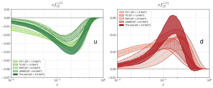
Figure 1: The first transverse moment $xf_{1T}^{\perp(1)}$ of the Sivers TMD as a function of $x$ for the up (left panel) and down quark (right panel). Solid band: the 68% confidence interval obtained in this work at $Q^{2}=4$ GeV². Hatched bands from PV11 [15], EIKV [17], TC18 [18], JAM20 [20] parametrizations, and at different $Q^{2}$ as indicated in the figure.

In Fig. 1, we show the first transverse moment $xf_{1T}^{\perp(1)}$ (Eq. (9), multiplied by $x$) as a function of $x$ at $Q_{0}=2$ GeV for the up (left panel) and down quark (right panel). We compare our results (solid band) with other parametrizations available in the literature [15, 17, 18, 20] (hatched bands, as indicated in the figure). In agreement with previous studies, the distribution for the up quark is negative, while for the down quark is positive and both have a similar magnitude. The Sivers function for sea quarks is very small and compatible with zero.

The authors of Ref. [21] also find results very similar to the ones in Fig. 1 when they fit the same SIDIS data and COMPASS Drell–Yan data with pion beams [58]. In this case, they also compute predictions for $W^{\pm}$ and $Z^{0}$ production at STAR kinematics which are very close to our fitted bands displayed in Fig. 8. Their strategy is very similar to the one adopted in this work but at higher perturbative accuracy, although their unpolarized TMDs are not obtained from an actual fit. However, when they include the STAR data in the global fit they artificially increase the statistical weight of those data by a factor $\sim 13$. Their global $\chi^{2}$ largely deteriorates and the uncertainty on the Sivers function significantly increases. Our finding is that because of large experimental errors STAR data does not affect much our final results when including them in the global fit, as discussed in detail in B.

The authors of Ref. [23] also perform a consistent extraction of both unpolarized and Sivers TMDs, and build contour plots of the density distribution in Eq. (1) similar to Fig. 2. A direct comparison is more difficult because the evolution of TMDs is achieved in a different framework, and the classification of the perturbative accuracy does not match the standard described in Ref. [10]. The displayed $x$-dependence of their Qiu-Sterman function (or related first $k_{T}$-moment of the Sivers function as in Eq. (9)) is roughly similar, at least for up and down quarks. However, the sea-quark channel shows large oscillations at large $x$, which entail a strong breaking of the positivity constraint of Eq. (20).

In general, the result of a fit is biased whenever a specific fitting functional form is chosen at the initial scale. In our case, we tried to reduce this bias by adopting a flexible functional form, as it is evident particularly in Eq. (23). Nevertheless, we stress that our extraction is still affected by this bias and extrapolations outside the range where data exist ($0.01\lesssim x\lesssim 0.3$) should be taken with due care. At variance with previous studies, in the denominator of the asymmetries in Eqs. (4) and (12) we are using unpolarized TMDs that were extracted from data in our previous Pavia17 fit, with their own uncertainties. Therefore, our uncertainty bands in Fig. 1 represent a realistic estimate of the statistical error of the Sivers function.

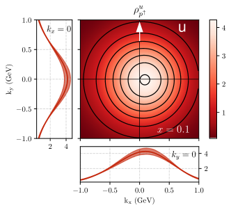
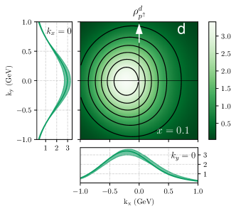
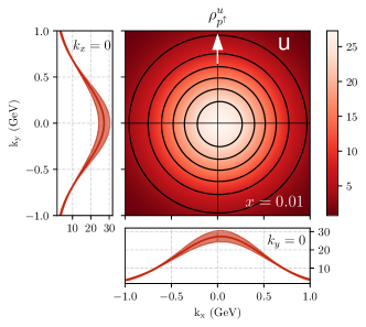
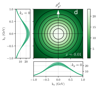
Figure 2: The density distribution $\rho_{p^{\uparrow}}^{a}$ of an unpolarized quark with flavor $a$ in a proton polarized along the $+y$ direction and moving towards the reader, as a function of $(k_{x},k_{y})$ at $Q^{2}=4$ GeV². Left panels for the up quark, right panels for the down quark. Upper panels for results at $x=0.1$, lower panels at $x=0.01$. For each panel, lower ancillary plots represent the 68% uncertainty band of the distribution at $k_{y}=0$ (where the effect of the distortion due to the Sivers function is maximal) while left ancillary plots at $k_{x}=0$ (where the distribution is the same as for an unpolarized proton). Results in the contour plots and the solid lines in the projections correspond to replica 105 (see text).

In Fig. 2, we show the density distribution $\rho^{a}_{p^{\uparrow}}$ of an unpolarized quark $a$ in a transversely polarized proton defined in Eq. (1), at $x=0.1$ (upper panels) and $x=0.01$ (lower panels) and at the scale $Q^{2}=4$ GeV². The proton is moving towards the reader and is polarized along the $+y$ direction. Since the up Sivers function is negative, the induced distortion is positive along the $+x$ direction for the up quark (left panels), and opposite for the down quark (right panels).

At $x=0.1$ the distortion due to the Sivers effect is evident, since we are close to the maximum value of the function shown in Fig. 1. The distortion is more pronounced for down quarks, because the Sivers function is larger and at the same time the unpolarized TMD is smaller. The peak positions are approximately $(k_{x})_{\text{max}}\approx 0.1$ GeV for up quarks and $-0.15$ GeV for down quarks. At lower values of $x$, the distortion disappears. These plots suggest that a virtual photon hitting a transversely polarized proton effectively “sees” more up quarks to its right and more down quarks to its left in momentum space.

The existence of this distortion requires two ingredients. First of all, the wavefunction describing quarks inside the proton must have a component with nonvanishing angular momentum. Secondly, effects due to final state interactions should be present [59], which in Feynman gauge can be described as the exchange of Coulomb gluons between the quark and the rest of the proton [60]. In simplified models [61], it is possible to separate these two ingredients and obtain an estimate of the angular momentum carried by each quark [62]. It turns out that up quarks give almost 50% contribution to the proton’s spin, while all other quarks and antiquarks give less than 10% [15]. We will leave this model-dependent study to a future publication. A model-independent estimate of quark angular momentum requires the determination of parton distributions that depend simultaneously on momentum and position [63, 64]. Nevertheless, the study of TMDs, and of the Sivers function in particular, can provide important constraints on models of the nucleon [65] and test lattice QCD computations [66].

In the near future, more data are expected from experiments at Jefferson Laboratory and CERN. Pioneering measurements in Drell-Yan processes with pion beams have been already reported [58], but they are not included in the present analysis because we do not have yet a consistent description of quark unpolarized TMDs in a pion. In the longer term, the recently approved Electron Ion Collider project [3, 4] will provide a large amount of data in different kinematic regions compared to present experiments [67]. With this abundance of data, we will be able to reduce the error bands, extend the range of validity of the extractions to lower and higher values of $x$, and obtain a much more detailed knowledge of the 3-dimensional distribution of partons in momentum space.

Appendix A Details about the fitting functional form

The functional form we chose to parametrize the Sivers function is built in order to automatically satisfy the positivity bound

$$\left[\frac{k_{T}^{2}}{2M^{2}}\,f_{1T}^{\perp}(x,k_{T}^{2})\right]^{2}\leq\frac{k_{T}^{2}}{4M^{2}}f_{1}^{2}(x,k_{T}^{2})\;.$$ (26)

It is given by

$$f_{1T}^{\perp a}(x,k_{T}^{2};Q_{0}^{2})=f_{1T}^{\perp(1)a}(x;Q_{0}^{2})\,f_{1T\mathrm{NP}}^{\perp}(x,k_{T}^{2})\;,$$ (27)

with

$$f_{1T\mathrm{NP}}^{\perp}(x,k_{T}^{2})=\frac{(1+\lambda_{S}\,k_{T}^{2})\,e^{-k_{T}^{2}/M_{1}^{2}}}{\pi K(x)\,(M_{1}^{2}+\lambda_{S}M_{1}^{4})}\,f_{1\mathrm{NP}}(x,k_{T}^{2})\;.$$ (28)

The $f_{1\mathrm{NP}}$ is the nonperturbative part of the unpolarized TMD $f_{1}$ and is taken from the Pavia17 extraction [1]:

$$f_{1\mathrm{NP}}(x,k_{T}^{2})=\frac{1}{\pi}\frac{1+\lambda k_{T}^{2}}{g_{1}(x)+\lambda g_{1}^{2}(x)}e^{-k_{T}^{2}/g_{1}(x)},$$ (29)

with

$$g_{1}(x) =N_{1}\;\frac{(1-x)^{\alpha}\ x^{\sigma}}{(1-\hat{x})^{\alpha}\ \hat{x}^{\sigma}}\,,\qquad\hat{x}=0.1\,.$$ (30)

The distributions of values for the parameters $N_{1}$, $\alpha$, $\sigma$, $\lambda$ are obtained from the Pavia17 fit and can be found in the NangaParbat repository . For convenience, we report here the values for the relevant replica 105

$$N_{1} =0.285\ {\rm GeV}^{2}, \alpha =2.98, \sigma =0.173, \lambda =0.39\ {\rm GeV}^{-2}\;.$$ (31)

In Eq. (28), the $M_{1},\,\lambda_{S}$ are free parameters. The $K(x)$ is a normalization factor to guarantee that the weighted integral of $f_{1T{\rm NP}}^{\perp}$ is 1 and the proper definition of the first $k_{T}$-moment of the Sivers function is recovered in Eq. (27). It is given by

$$K(x) \equiv\pi\int dk_{T}^{2}\frac{k_{T}^{2}}{2M^{2}}\frac{\Big{(}1+\lambda_{S}k_{T}^{2}\Big{)}}{\pi\Big{(}M_{1}^{2}+\lambda_{S}M_{1}^{4}\Big{)}}e^{-k_{T}^{2}/M_{1}^{2}}\frac{(1+\lambda k_{T}^{2})}{\pi\Big{(}g_{1}(x)+\lambda[g_{1}(x)]^{2}\Big{)}}e^{-k_{T}^{2}/g_{1}(x)}$$ (32)

$$=\,\frac{g_{1}(x)\,M_{1}^{2}}{2\pi M^{2}\Big{(}1+\lambda g_{1}(x)\Big{)}\,\Big{(}g_{1}(x)+M_{1}^{2}\Big{)}^{2}\,\Big{(}1+\lambda_{S}M_{1}^{2}\Big{)}}\,\left[1+2(\lambda+\lambda_{S})\,\frac{g_{1}(x)\,M_{1}^{2}}{g_{1}(x)+M_{1}^{2}}+6\lambda\lambda_{S}\,\left(\frac{g_{1}(x)\,M_{1}^{2}}{g_{1}(x)+M_{1}^{2}}\right)^{2}\right]\;.$$

The Fourier transform of $f_{1T\mathrm{NP}}^{\perp}$ in Eq. (28) reads

$$\widetilde{f}_{1T{\rm NP}}^{\perp}(x,b_{T}^{2}) =\pi\int dk_{T}^{2}\,J_{0}(k_{T}b_{T})\,f_{1T{\rm NP}}^{\perp}(x,k_{T}^{2})=\frac{\exp\left(-\frac{b_{T}^{2}}{4}\,\frac{g_{1}M_{1}^{2}}{g_{1}+M_{1}^{2}}\right)}{\pi\,K(x)\,\Big{(}1+\lambda_{S}M_{1}^{2}\Big{)}\,\Big{(}1+\lambda g_{1}\Big{)}\,\Big{(}g_{1}+M_{1}^{2}\Big{)}}$$

$$\!\!\!\!\!\!\!\!\times\Bigg{\{}1+\left(\lambda+\lambda_{S}+2\lambda\lambda_{S}\frac{g_{1}M_{1}^{2}}{g_{1}+M_{1}^{2}}\right)\,\frac{g_{1}M_{1}^{2}}{g_{1}+M_{1}^{2}}\,\left(1-\frac{b_{T}^{2}}{4}\,\frac{g_{1}M_{1}^{2}}{g_{1}+M_{1}^{2}}\right)-\frac{b_{T}^{2}}{2}\,\left(\frac{g_{1}M_{1}^{2}}{g_{1}+M_{1}^{2}}\right)^{3}\,\lambda\lambda_{S}\,\left(1-\frac{b_{T}^{2}}{8}\,\frac{g_{1}M_{1}^{2}}{g_{1}+M_{1}^{2}}\right)\,\Bigg{\}}$$

$$=\frac{2M^{2}\,(g_{1}+M_{1}^{2})\,\exp\left(-\frac{b_{T}^{2}}{4}\,\frac{g_{1}M_{1}^{2}}{g_{1}+M_{1}^{2}}\right)}{g_{1}M_{1}^{2}\,\left[1+\left(\lambda+\lambda_{S}+3\lambda\lambda_{S}\,\frac{g_{1}M_{1}^{2}}{g_{1}+M_{1}^{2}}\right)\,2\,\frac{g_{1}M_{1}^{2}}{g_{1}+M_{1}^{2}}\right]}$$

$$\!\!\!\!\!\!\!\!\times\Bigg{\{}1+\left(\lambda+\lambda_{S}+2\lambda\lambda_{S}\frac{g_{1}M_{1}^{2}}{g_{1}+M_{1}^{2}}\right)\,\frac{g_{1}M_{1}^{2}}{g_{1}+M_{1}^{2}}\,\left(1-\frac{b_{T}^{2}}{4}\,\frac{g_{1}M_{1}^{2}}{g_{1}+M_{1}^{2}}\right)-\frac{b_{T}^{2}}{2}\,\left(\frac{g_{1}M_{1}^{2}}{g_{1}+M_{1}^{2}}\right)^{3}\,\lambda\lambda_{S}\,\left(1-\frac{b_{T}^{2}}{8}\,\frac{g_{1}M_{1}^{2}}{g_{1}+M_{1}^{2}}\right)\,\Bigg{\}}\;.$$ (33)

The first transverse moment is parametrized as

$$\begin{split}f_{1T}^{\perp(1)a}&(x;Q_{0}^{2})=\frac{N_{\mathrm{Siv}}^{a}}{G_{\mathrm{max}}^{a}}\,K(x)\,x^{\alpha_{a}}(1-x)^{\beta_{a}}\left[1+A_{a}\,T_{1}(x)+B_{a}\,T_{2}(x)\right]\,f_{1}^{a}(x;Q_{0}^{2})\,,\end{split}$$ (34)

where $T_{n}(x)$ are Chebyshev polynomials of order $n$, and the unpolarized collinear parton densities $f_{1}^{a}$ are taken from the GJR parametrization [47], consistently with the Pavia17 fit. The flavor-dependent factor $G_{\mathrm{max}}^{a}$ is defined as

$$G_{\mathrm{max}}^{a}=\max_{k_{T}}\Biggl{[}\frac{k_{T}}{\pi M}\,\biggl{|}\frac{1+\lambda_{S}k_{T}^{2}}{M_{1}^{2}+\lambda_{S}M_{1}^{4}}\biggr{|}\,e^{-k_{T}^{2}/M_{1}^{2}}\Biggr{]}\;\max_{x}\Biggl{[}x^{\alpha_{a}}(1-x)^{\beta_{a}}\,\bigl{|}1+A_{a}\,T_{1}(x)+B_{a}\,T_{2}(x)\bigr{|}\,\Biggr{]}\;.$$ (35)

Together with the constraint $|N_{\mathrm{Siv}}^{a}|\leq 1$, it is introduced into Eq. (34) to guarantee that the Sivers function of Eq. (27) satisfies the positivity condition of Eq. (26). For the relevant replica 105 we have

$$G_{\mathrm{max}}^{u} =1.99\times 10^{-2}, G_{\mathrm{max}}^{d} =5.58\times 10^{-4}, G_{\mathrm{max}}^{s} =2.42\times 10^{-3}.$$ (36)

Appendix B Comparison with data

In this section, we present figures showing the quality of our fit. In all plots, our results are represented by solid bands whenever data points are actually included in the fit, while hatched bands are predictions for the same measurements projected over different kinematic variables. The predictions are obtained by integrating upon the variables over which they are not projected.

In Fig. 3, we report the results for the COMPASS 2009 run [49] (32 points with $\chi^{2}=26.5\pm 4.2$), while in Fig. 4 and Fig. 5 we show the 2017 run for positive and negative final state hadrons, respectively [50] (50 points with $\chi^{2}=31.3\pm 3.8$). The results for JLab [51] are depicted in Fig. 6 (6 points with $\chi^{2}=4.1\pm 0.7$). The HERMES results [48], together with predictions of projections on different variables, are shown in Fig. 7 (30 points with $\chi^{2}=46.2\pm 3.8$). Finally, Fig. 8 contains the results for $W^{\pm}$ and $Z^{0}$ production measured by the STAR Collaboration [52] (7 points with $\chi^{2}=13.97\pm 0.6$).

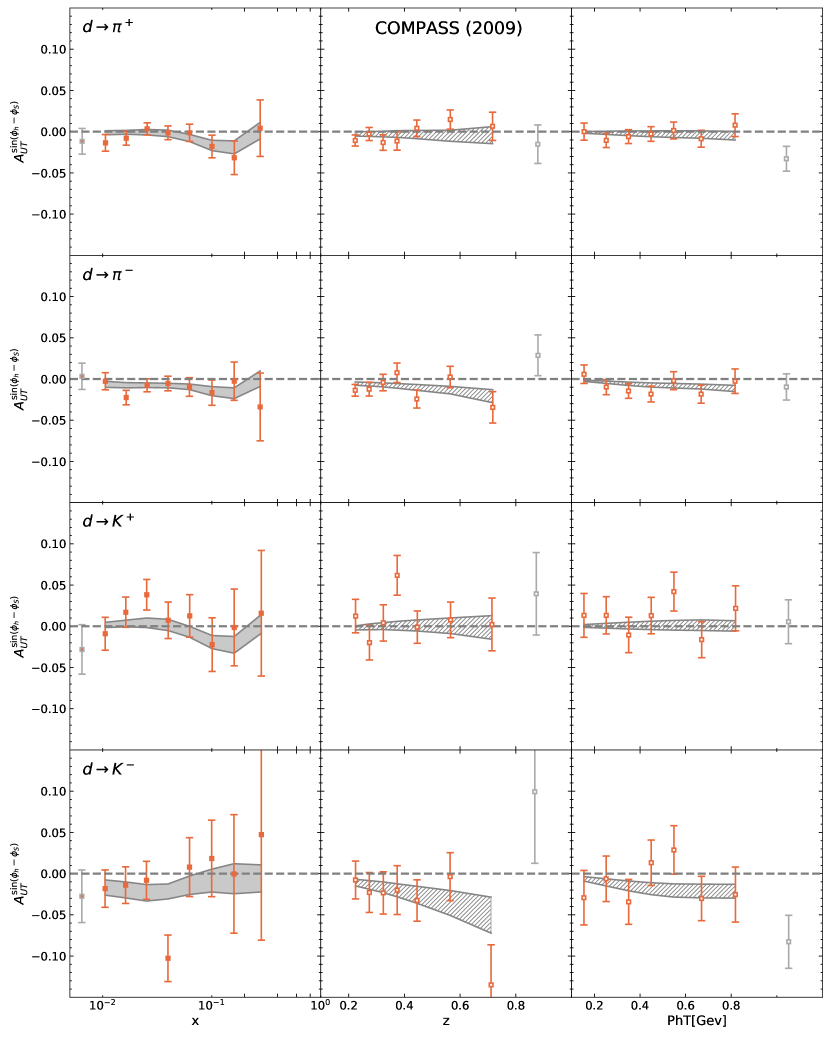
Figure 3: COMPASS 2009 Sivers asymmetries from SIDIS off a deuteron target (⁶LiD) with production of $\pi^{+}$, $\pi^{-}$, $K^{+}$, $K^{-}$ in the final state [49], presented as function of $x$, $z$, $P_{hT}$. Only the $x$-dependent projections have been included in the fit (solid bands), the dependence on other variables is predicted (hatched bands).

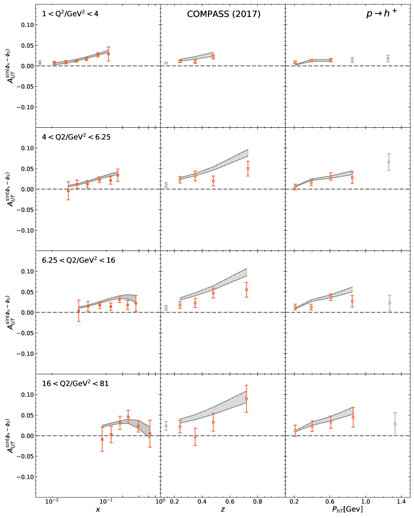
Figure 4: COMPASS 2017 Sivers asymmetries from SIDIS off a proton target (NH₃) with production of positive hadrons $h^{+}$ [50], presented as function of $x$, $z$, $P_{hT}$ and divided in four different $Q^{2}$ bins. Same notation as in previous figure.

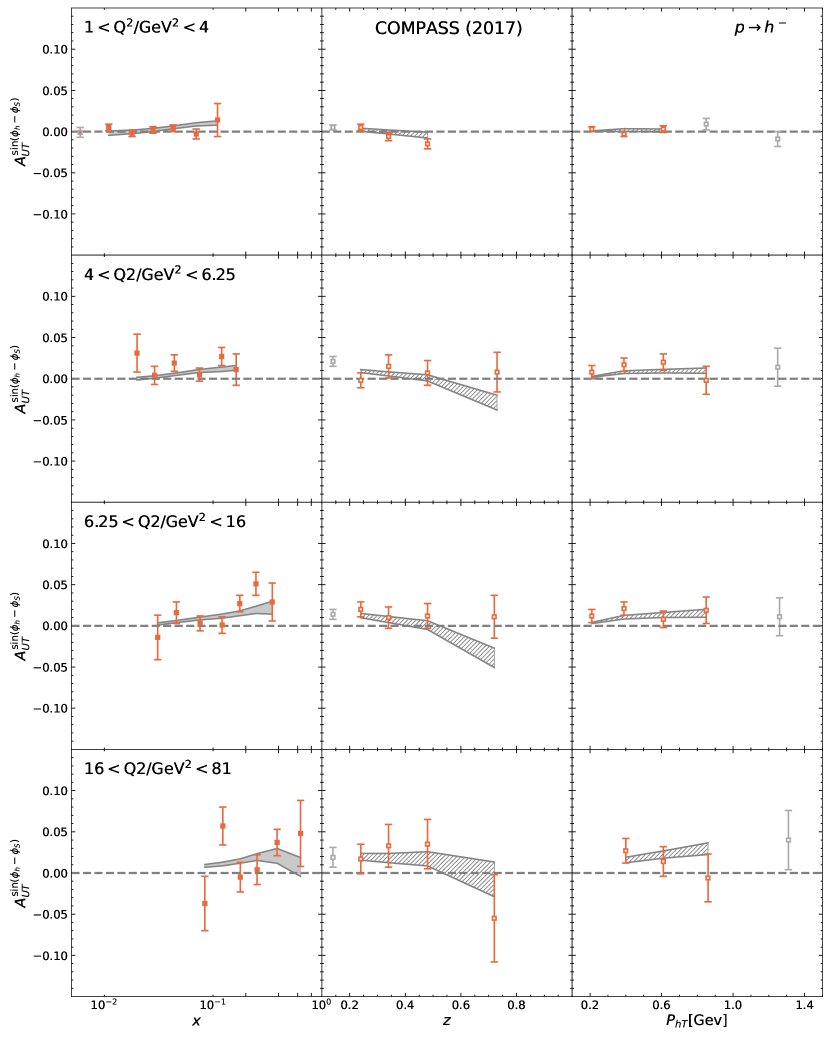
Figure 5: COMPASS 2017 Sivers asymmetries from SIDIS off a proton target (NH₃) with production of negative hadrons $h^{-}$ [50], presented as function of $x$, $z$, $P_{hT}$ and divided in four different $Q^{2}$ bins. Same notation as in Fig. 3.

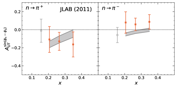
Figure 6: JLab Sivers asymmetries from SIDIS off a deuteron target (⁶LiD) with production of positive and negative $\pi$ in the final state [51], presented as function of $x$. Same notation as in Fig. 3.

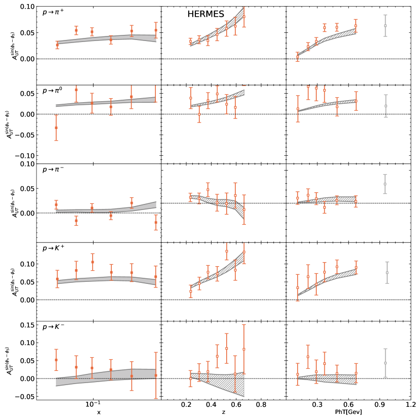
Figure 7: HERMES Sivers asymmetries from SIDIS off a proton target (H) with production of $\pi^{+}$, $\pi^{0}$, $\pi^{-}$, $K^{+}$, $K^{-}$ in the final state [48], presented as a function of $x$, $z$, $P_{hT}$. Same notation as in Fig. 3.

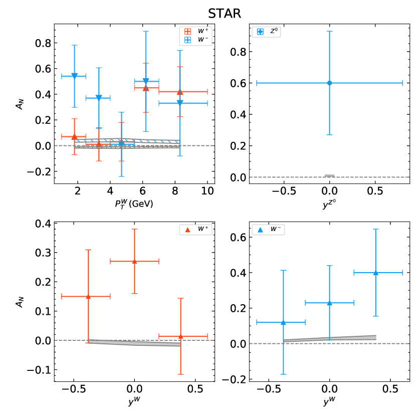
Figure 8: STAR Sivers asymmetries from $p-p^{\uparrow}$ collisions producing $W^{\pm}$ and $Z^{0}$ in the final state [52], presented as function of rapidity $y$ and $p_{T}^{W}$. Same notation as in Fig. 3.

References

Bacchetta et al. [2017]
A. Bacchetta,
F. Delcarro,
C. Pisano,
M. Radici, and
A. Signori,
JHEP 06, 081
(2017), [Erratum: JHEP06,051(2019)].
Sivers [1990]
D. W. Sivers,
Phys. Rev. D41,
83 (1990).
Boer et al. [2011a]
D. Boer et al.
(2011a), arXiv:1108.1713 [nucl-th].
Accardi et al. [2016]
A. Accardi et al.,
Eur. Phys. J. A52,
268 (2016).
Dudek et al. [2012]
J. Dudek et al.,
Eur. Phys. J. A48,
187 (2012).
Aschenauer et al. [2016]
E.-C. Aschenauer
et al. (2016), arXiv:1602.03922 [nucl-ex].
Bacchetta et al. [2004]
A. Bacchetta,
U. D’Alesio,
M. Diehl, and
C. A. Miller,
Phys. Rev. D70,
117504 (2004).
Bertone et al. [2019]
V. Bertone,
I. Scimemi, and
A. Vladimirov,
JHEP 06, 028
(2019).
Scimemi and Vladimirov [2020]
I. Scimemi and
A. Vladimirov,
JHEP 06, 137
(2020).
Bacchetta et al. [2020]
A. Bacchetta,
V. Bertone,
C. Bissolotti,
G. Bozzi,
F. Delcarro,
F. Piacenza, and
M. Radici,
JHEP 07, 117
(2020).
Anselmino et al. [2005]
M. Anselmino,
M. Boglione,
U. D’Alesio,
A. Kotzinian,
F. Murgia, and
A. Prokudin,
Phys. Rev. D72,
094007 (2005), [Erratum:
Phys. Rev.D72,099903(2005)].
Collins et al. [2006]
J. C. Collins,
A. V. Efremov,
K. Goeke,
S. Menzel,
A. Metz, and
P. Schweitzer,
Phys. Rev. D73,
014021 (2006).
Vogelsang and Yuan [2005]
W. Vogelsang and
F. Yuan,
Phys. Rev. D72,
054028 (2005).
Anselmino et al. [2009]
M. Anselmino,
M. Boglione,
U. D’Alesio,
A. Kotzinian,
S. Melis,
F. Murgia,
A. Prokudin, and
C. Turk,
Eur. Phys. J. A39,
89 (2009).
Bacchetta and Radici [2011]
A. Bacchetta and
M. Radici,
Phys. Rev. Lett. 107,
212001 (2011).
Sun and Yuan [2013]
P. Sun and
F. Yuan,
Phys. Rev. D 88,
114012 (2013).
Echevarria et al. [2014]
M. G. Echevarria,
A. Idilbi,
Z.-B. Kang, and
I. Vitev,
Phys. Rev. D89,
074013 (2014).
Boglione et al. [2018]
M. Boglione,
U. D’Alesio,
C. Flore, and
J. O. Gonzalez-Hernandez,
JHEP 07, 148
(2018).
Luo and Sun [2020]
X. Luo and
H. Sun,
Phys. Rev. D101,
074016 (2020).
Cammarota et al. [2020]
J. Cammarota,
L. Gamberg,
Z.-B. Kang,
J. A. Miller,
D. Pitonyak,
A. Prokudin,
T. C. Rogers,
and N. Sato
(2020), arXiv:2002.08384 [hep-ph].
Echevarria et al. [2021]
M. G. Echevarria,
Z.-B. Kang, and
J. Terry,
JHEP 01, 126
(2021).
Bury et al. [2021a]
M. Bury,
A. Prokudin, and
A. Vladimirov,
Phys. Rev. Lett. 126,
112002 (2021a).
Bury et al. [2021b]
M. Bury,
A. Prokudin, and
A. Vladimirov,
JHEP 05, 151
(2021b).
Bacchetta et al. [2007]
A. Bacchetta,
M. Diehl,
K. Goeke,
A. Metz,
P. J. Mulders,
and M. Schlegel,
JHEP 02, 093
(2007).
Boer et al. [2011b]
D. Boer,
L. Gamberg,
B. Musch, and
A. Prokudin,
JHEP 10, 021
(2011b).
Qiu and Sterman [1999]
J.-w. Qiu and
G. F. Sterman,
Phys. Rev. D59,
014004 (1999).
Boer et al. [2003]
D. Boer,
P. J. Mulders,
and F. Pijlman,
Nucl. Phys. B667,
201 (2003).
Ji et al. [2006]
X. Ji,
J.-W. Qiu,
W. Vogelsang,
and F. Yuan,
Phys. Rev. Lett. 97,
082002 (2006).
Scimemi et al. [2019]
I. Scimemi,
A. Tarasov, and
A. Vladimirov,
JHEP 05, 125
(2019).
Ebert et al. [2022]
M. A. Ebert,
J. K. L. Michel,
I. W. Stewart,
and Z. Sun
(2022), arXiv:2201.07237 [hep-ph].
Arnold et al. [2009]
S. Arnold,
A. Metz, and
M. Schlegel,
Phys. Rev. D 79,
034005 (2009).
Zyla et al. [2020]
P. A. Zyla et al.
(Particle Data Group), PTEP
2020, 083C01
(2020).
Collins et al. [1985]
J. C. Collins,
D. E. Soper, and
G. F. Sterman,
Nucl. Phys. B250,
199 (1985).
Bozzi et al. [2011]
G. Bozzi,
S. Catani,
G. Ferrera,
D. de Florian,
and M. Grazzini,
Phys. Lett. B 696,
207 (2011).
Boer and den Dunnen [2014]
D. Boer and
W. J. den Dunnen,
Nucl. Phys. B 886,
421 (2014).
Collins et al. [2016]
J. Collins,
L. Gamberg,
A. Prokudin,
T. C. Rogers,
N. Sato, and
B. Wang,
Phys. Rev. D 94,
034014 (2016).
Salam and Rojo [2009]
G. P. Salam and
J. Rojo,
Comput. Phys. Commun. 180,
120 (2009).
Kang and Qiu [2009]
Z.-B. Kang and
J.-W. Qiu,
Phys. Rev. D 79,
016003 (2009).
Braun et al. [2009]
V. M. Braun,
A. N. Manashov,
and B. Pirnay,
Phys. Rev. D 80,
114002 (2009), [Erratum:
Phys.Rev.D 86, 119902 (2012)].
Vogelsang and Yuan [2009]
W. Vogelsang and
F. Yuan,
Phys. Rev. D 79,
094010 (2009).
Zhou et al. [2009]
J. Zhou,
F. Yuan, and
Z.-T. Liang,
Phys. Rev. D 79,
114022 (2009).
Kang and Qiu [2012]
Z.-B. Kang and
J.-W. Qiu,
Phys. Lett. B 713,
273 (2012).
Schafer and Zhou [2012]
A. Schafer and
J. Zhou,
Phys. Rev. D 85,
117501 (2012).
Bacchetta et al. [2000]
A. Bacchetta,
M. Boglione,
A. Henneman, and
P. J. Mulders,
Phys. Rev. Lett. 85,
712 (2000).
Bhattacharya et al. [2021]
S. Bhattacharya,
Z.-B. Kang,
A. Metz,
G. Penn, and
D. Pitonyak
(2021), arXiv:2110.10253 [hep-ph].
Gluck et al. [2008]
M. Gluck,
P. Jimenez-Delgado,
and E. Reya,
Eur. Phys. J. C53,
355 (2008).
Airapetian et al. [2009]
A. Airapetian
et al. (HERMES),
Phys. Rev. Lett. 103,
152002 (2009).
Alekseev et al. [2009]
M. Alekseev et al.
(COMPASS), Phys. Lett.
B673, 127 (2009).
Adolph et al. [2017]
C. Adolph et al.
(COMPASS), Phys. Lett.
B770, 138 (2017).
Qian et al. [2011]
X. Qian et al.
(Jefferson Lab Hall A), Phys. Rev.
Lett. 107, 072003
(2011).
Adamczyk et al. [2016]
L. Adamczyk et al.
(STAR), Phys. Rev. Lett.
116, 132301
(2016).
Forte et al. [2002]
S. Forte,
L. Garrido,
J. I. Latorre,
and A. Piccione,
JHEP 05, 062
(2002).
Ball et al. [2010a]
R. D. Ball,
L. Del Debbio,
S. Forte,
A. Guffanti,
J. I. Latorre,
J. Rojo, and
M. Ubiali,
Nucl. Phys. B838,
136 (2010a).
Radici et al. [2015]
M. Radici,
A. Courtoy,
A. Bacchetta,
and
M. Guagnelli,
JHEP 05, 123
(2015).
Ball et al. [2010b]
R. D. Ball,
L. Del Debbio,
S. Forte,
A. Guffanti,
J. I. Latorre,
J. Rojo, and
M. Ubiali
(NNPDF), JHEP
05, 075
(2010b).
Signori et al. [2013]
A. Signori,
A. Bacchetta,
M. Radici, and
G. Schnell,
JHEP 1311, 194
(2013).
Aghasyan et al. [2017]
M. Aghasyan et al.
(COMPASS), Phys. Rev. Lett.
119, 112002
(2017).
Brodsky et al. [2002]
S. J. Brodsky,
D. S. Hwang, and
I. Schmidt,
Phys. Lett. B530,
99 (2002).
Ji and Yuan [2002]
X.-d. Ji and
F. Yuan,
Phys. Lett. B543,
66 (2002).
Pasquini et al. [2019]
B. Pasquini,
S. Rodini, and
A. Bacchetta,
Phys. Rev. D100,
054039 (2019).
Burkardt [2002]
M. Burkardt,
Phys. Rev. D66,
114005 (2002).
Ji [1997]
X.-D. Ji,
Phys. Rev. Lett. 78,
610 (1997).
Lorce et al. [2012]
C. Lorce,
B. Pasquini,
X. Xiong, and
F. Yuan,
Phys. Rev. D85,
114006 (2012).
Burkardt and Pasquini [2016]
M. Burkardt and
B. Pasquini,
Eur. Phys. J. A52,
161 (2016).
Yoon et al. [2017]
B. Yoon,
M. Engelhardt,
R. Gupta,
T. Bhattacharya,
J. R. Green,
B. U. Musch,
J. W. Negele,
A. V. Pochinsky,
A. Schäfer, and
S. N. Syritsyn,
Phys. Rev. D96,
094508 (2017).
Abdul Khalek et al. [2021]
R. Abdul Khalek
et al. (2021), arXiv:2103.05419
[physics.ins-det].