The Lyapunov exponents and the neighbourhood of periodic orbits

Abstract

We show that the Lyapunov exponents of a periodic orbit can be easily obtained from the eigenvalues of the monodromy matrix. It turns out that the Lyapunov exponents of simply stable periodic orbits are all zero, simply unstable periodic orbits have only one positive Lyapunov exponent, doubly unstable periodic orbits have two different positive Lyapunov exponents and the two positive Lyapunov exponents of complex unstable periodic orbits are equal. We present a numerical example for periodic orbits in a realistic galactic potential. Moreover, the center manifold theorem allowed us to show that stable, simply unstable and doubly unstable periodic orbits are the mothers of families of, respectively, regular, partially and fully chaotic orbits in their neighbourhood.

1 Introduction

In several previous articles (Muzzio, Carpintero & Wachlin, 2005; Muzzio, 2006; Muzzio, Navone & Zorzi, 2009; Zorzi & Muzzio, 2012; Carpintero, Muzzio & Navone, 2014; Carpintero & Muzzio, 2016) we have investigated the role that chaos plays in the dynamics of stellar systems. Since these systems can be described by autonomous Hamiltonians, their orbits have always two Lyapunov exponents equal to zero, and the remaining four are always two pairs of opposite real numbers (e.g., Benettin et al., 1976). This means that there may be zero, one or two positive Lyapunov exponents. No positive Lyapunov exponents means that there is no direction in phase space along which two initially infinitesimally separated orbits diverge exponentially, that is, the original orbit is regular. Otherwise, the orbit is chaotic. But chaotic orbits are evidently not all the same: there are those with only one positive Lyapunov exponent, called partially chaotic orbits, and those with two positive Lyapunov exponents, called fully chaotic orbits. One of the main results from our abovementioned works was that fully chaotic orbits are a disjoint family from the partially chaotic orbits, even in their spatial distribution inside the system.

Contopoulos, Galgani & Giorgilli (1978) and Pettini & Vulpiani (1984) had also reported the finding of partially chaotic orbits in other autonomous Hamiltonian systems, but their existence was denied by Froeschlé (1970, 1971) and by Lichtenberg & Lieberman (1992). Nevertheless, more recently, Muzzio (2017, 2018) proved their existence over, at least, time intervals of 50 million Hubble times.

On the other hand, studies of the stability of periodic orbits in the three-body problem (Hadjidemetriou, 1975) and in triaxial potentials (Magnenat, 1982; Contopoulos & Magnenat, 1985; Contopoulos, 2002) have yielded a wealth of phenomena of interest. The different classes of instability of these orbits are determined according to the eigenvalues of the monodromy matrix of the periodic orbit. In particular, Contopoulos & Magnenat (1985) have classified the orbits into four categories: stable, unstable, doubly unstable and complex unstable. The question naturally arises of whether these orbits are somehow related to the regular, partially and fully chaotic orbits. Therefore, we decided to investigate the relationship between the eigenvalues of the monodromy matrix of periodic orbits and the Lyapunov exponents of those orbits and we found that, in fact, the latter can be computed from the former. Besides, the stability of the periodic orbits, influences decisively the phase space in their neighbourhood and it turns out that, just as stable periodic orbits are surrounded by regular orbits, simply unstable periodic orbits are surrounded by partially chaotic orbits and doubly and complex unstable periodic orbits are surrounded by fully chaotic orbits. The present paper presents our results. Section 2 gives our analytical proof, section 3 presents a numerical example and our conclusions are described in Section 4.

2 Lyapunov exponents and periodic motion

2.1 Lyapunov exponents as eigenvalues of the main fundamental matrix

In a 3D potential, a regular orbit is defined as an orbit which obeys al least three isolating integrals of motion (e.g., Binney & Tremaine, 2008); otherwise, it is irregular. On the other hand, a chaotic orbit is defined as an orbit which has sensitivity to the initial conditions, that is, if its initial phase space position $\textbf{{w}}_{0}\equiv(\textbf{{x}}_{0},\textbf{{v}}_{0})$ is infinitesimally perturbed, then the new orbit (hereafter called perturbed orbit) diverges exponentially from the original one. Though there is no proof that every irregular orbit is chaotic, we will stick to the widespread custom of considering both sets as the same.

The standard gauge to measure the rate of divergence between an orbit and its perturbed sister is the set of Lyapunov exponents, sometimes called Lyapunov characteristic numbers or Lyapunov characteristic exponents. If we choose six independent directions of the phase space $\textbf{{e}}_{i}$, $i=1,\dots,6$, and perturb the initial conditions in the direction $j$ by the amount $\delta w_{j}(0)$, then the Lyapunov exponents are defined by (e.g., Lichtenberg & Lieberman, 1992)

$$\lambda_{i}=\lim_{t\to\infty}{1\over t}\ln{|\delta w_{i}(t)|\over|\delta w_{i}(0)|},\quad i=1,\dots,6,$$ (1)

where $\delta w_{i}(t)$ is the component of the deviation at time $t$ of the initial $i$th component of the deviation $\delta w_{i}(0)$, and the norm $|\cdot|$ is any norm of the phase space, normally the Euclidean one.

Numerically, the deviation $\delta\textbf{{w}}(t)$ can be computed starting from the equations of motion

$$\textbf{{\.{w}}}=\textbf{{F}}(\textbf{{w}}),$$ (2)

where $\textbf{{w}}(t)$ is the phase point of the orbit, $\textbf{{\.{w}}}(t)$ its velocity, and F are the functions that define the dynamical system. Developing Eqs. (2) in a Taylor series around the unperturbed orbit and retaining only the first order, we obtain the so called variational equations:

$${\text{d}\over\text{d}t}(\delta\textbf{{w}})=\left.{\partial\textbf{{F}}\over\partial\textbf{{w}}}\right|_{\textbf{{w}}}\cdot\delta\textbf{{w}}.$$ (3)

The set of variational equations (3) for the six components of the deviation is, then, a system of linear, homogeneous, ordinary differential equations. For this kind of systems, a fundamental matrix $\textbf{{S}}(t)$ is defined as a matrix whose columns are linearly independent solutions of the system (e.g., Roxin & Spinadel, 1976). In our case,

$$\textbf{{S}}(t)=(\delta\textbf{{w}}_{1},\dots,\delta\textbf{{w}}_{6}),$$ (4)

where each $\delta\textbf{{w}}_{i}$ is an independent solution of Eq. (3) and represents a column, is the fundamental matrix of the variational equations. It is then clear that

$$\textbf{{\.{S}}}(t)=\left.{\partial\textbf{{F}}\over\partial\textbf{{w}}}\right|_{\textbf{{w}}}\cdot\textbf{{S}}(t).$$ (5)

Since the $\delta\textbf{{w}}_{i}$ are linearly independent solutions, then

$$\textbf{{S}}\cdot\textbf{{S}}^{\textsf{T}}=\text{diag}(|\delta\textbf{{w}}_{1}|^{2},\dots,|\delta\textbf{{w}}_{6}|^{2})=\textbf{{S}}^{2},$$ (6)

where $(\cdot)^{\textsf{T}}$ indicates transposition. If we choose $\textbf{{S}}(t)$ such that $\textbf{{S}}(0)=\textbf{{1}}$, i.e., the identity matrix (in which case $\textbf{{S}}(t)$ is called main fundamental matrix), Eq. (1) shows that the set of Lyapunov exponents can be expressed as the eigenvalues of a (diagonal) matrix L where

$$\textbf{{L}}=\lim_{t\to\infty}{1\over 2t}\ln(\textbf{{S}}^{2})=\lim_{t\to\infty}{1\over t}\ln|\textbf{{S}}|,$$ (7)

where $|\textbf{{S}}|=\text{diag}(|\delta\textbf{{w}}_{1}|,\dots,|\delta\textbf{{w}}_{6}|)$ (e.g., Benettin et al., 1980).

Now, let

$$\textbf{{w}}(t)=\textbf{{G}}(t,\textbf{{w}}_{0})$$ (8)

be the solution of Eq. (2) with initial condition $\textbf{{w}}(0)=\textbf{{w}}_{0}$, and let the matrix M be defined by

$$\textbf{{M}}(t)={\partial\textbf{{G}}(t,\textbf{{w}}_{0})\over\partial\textbf{{w}}_{0}}={\partial\textbf{{w}}(t)\over\partial\textbf{{w}}_{0}},$$ (9)

i.e. $\textbf{{M}}(t)$ is the matrix that evolves the initial perturbation until time $t$:

$$\delta\textbf{{w}}(t)=\textbf{{M}}(t)\cdot\delta\textbf{{w}}_{0}.$$ (10)

Now, by applying the chain rule, we have

$$\textbf{{\.{M}}}={\partial\textbf{{\.{w}}}\over\partial\textbf{{w}}_{0}}={\partial\textbf{{\.{w}}}\over\partial\textbf{{w}}}\cdot{\partial\textbf{{w}}\over\partial\textbf{{w}}_{0}}={\partial\textbf{{F}}\over\partial\textbf{{w}}}\cdot\textbf{{M}},$$ (11)

i.e., M turns out to be the fundamental matrix S of the variational equations (cf. Eq. (5)).

2.2 Lyapunov exponents of a periodic motion

We now specialise in periodic motion. Let the solution of Eq. (2) represent a periodic orbit of period $T$. The stability of such an orbit can be established studying the behavior of a second orbit obtained by perturbing the initial conditions, i.e. by integrating the variational equations. Let M be the fundamental matrix of this system; it satisfies (cf. Eq. (11))

$$\textbf{{\.{M}}}(t)=\left.{\partial\textbf{{\.{w}}}\over\partial\textbf{{w}}}\right|_{\textbf{{w}}}\cdot\textbf{{M}}(t).$$ (12)

According to the Floquet theorem (Floquet, 1883), the fundamental matrix $\textbf{{M}}(t)$ in this case is also periodic with period $T$. This property, along with Eq. (10) and the assumption that $\textbf{{M}}(0)=\textbf{{1}}$ allow us to write

$$\delta\textbf{{w}}(T)=\textbf{{M}}(T)\cdot\delta\textbf{{w}}(0).$$ (13)

The main fundamental matrix evaluated at $t=T$, $\textbf{{M}}(T)$, is called the monodromy matrix of the periodic orbit (e.g. Contopoulos, 2002).

Since the motion is periodic with period $T$, then

$$\begin{split}\delta\textbf{{w}}(2T)&=\textbf{{M}}(2T)\cdot\delta\textbf{{w}}(0)\\ &=\textbf{{M}}(T)\cdot\left[\textbf{{M}}(T)\cdot\delta\textbf{{w}}(0)\right]\\ &=\left[\textbf{{M}}(T)\right]^{2}\cdot\delta\textbf{{w}}(0),\end{split}$$ (14)

so we have, for $n\in{\mathbb{N}}$,

$$\textbf{{M}}(nT)=\left[\textbf{{M}}(T)\right]^{n}.$$ (15)

Then, the Lyapunov exponents can be easily computed as the natural logarithms of the eigenvalues of the monodromy matrix divided by $T$ (cf. Eq.(7)):

$$\begin{split}\textbf{{L}}&=\lim_{t\to\infty}{1\over t}\ln\left|\textbf{{M}}(t)\right|\\ &=\lim_{n\to\infty}{1\over nT}\ln\left|\textbf{{M}}(nT)\right|\\ &={1\over T}\ln\left|\textbf{{M}}(T)\right|,\end{split}$$ (16)

where in the last line we have used Eq. (15). If we let $\ell_{i}$, $i=1,\dots,6$ be the six eigenvalues of $\textbf{{M}}(T)$, then we have

$$\lambda_{i}={1\over T}\ln|\ell_{i}|.$$ (17)

As usual, the $\ell_{i}$’s are obtained as the six roots of the characteristic polynomial of $\textbf{{M}}(T)$,

$$a_{6}\ell^{6}+a_{5}\ell^{5}+a_{4}\ell^{4}+a_{3}\ell^{3}+a_{2}\ell^{2}+a_{1}\ell+a_{0}=0,$$ (18)

where the $a_{i}$ are real numbers. The two null Lyapunov exponents imply that two of the eigenvalues are always unity. After dividing by $(\ell-1)^{2}$, the remaining polynomial we write as

$$c_{4}\ell^{4}+c_{3}\ell^{3}+c_{2}\ell^{2}+c_{1}\ell+c_{0}=0.$$ (19)

We also know that the four remaining Lyapunov exponents come in pairs of opposite numbers, so the corresponding eigenvalues are pairs of reciprocal numbers. Let $\{\ell_{1},\ell_{2}=\ell_{1}^{-1},\ell_{3},\ell_{4}=\ell_{3}^{-1}\}$ be those eigenvalues. Then, the polynomial (19) can be written

$$\ell^{4}+\alpha\ell^{3}+\beta\ell^{2}+\alpha\ell+1=0,$$ (20)

where

$$\begin{split}\alpha&=-(\ell_{1}+\ell_{2}+\ell_{3}+\ell_{4}),\\ \beta&=\ell_{1}\ell_{3}+\ell_{1}\ell_{4}+\ell_{2}\ell_{3}+\ell_{2}\ell_{4}+2.\end{split}$$ (21)

Following the standard notation initiated by Hadjidemetriou (1975), we let

$$\begin{split}b_{1}&=-(\ell_{1}+\ell_{2}),\\ b_{2}&=-(\ell_{3}+\ell_{4}),\end{split}$$ (22)

with which

$$\begin{split}\alpha&=b_{1}+b_{2},\\ \beta&=b_{1}b_{2}+2,\end{split}$$ (23)

and, therefore,

$$\begin{split}b_{1}&={1\over 2}\left(\alpha+\sqrt{\Delta}\right),\\ b_{2}&={1\over 2}\left(\alpha-\sqrt{\Delta}\right),\end{split}$$ (24)

where

$$\Delta=\alpha^{2}-4(\beta-2).$$ (25)

With this notation, the four roots (eigenvalues) can be written as

$$\begin{split}\ell_{1,2}&={1\over 2}\left(-b_{1}\pm\sqrt{b_{1}^{2}-4}\right),\\ \ell_{3,4}&={1\over 2}\left(-b_{2}\pm\sqrt{b_{2}^{2}-4}\right).\end{split}$$ (26)

2.3 Stability of a periodic motion

Although the Lyapunov exponents of a periodic motion can be effortlessly computed from the eigenvalues of the monodromy matrix, the stability of its orbits is usually studied by considering $\Delta$, $b_{1}$ and $b_{2}$ (e.g. Hadjidemetriou, 1975; Magnenat, 1982; Contopoulos & Magnenat, 1985; Patsis & Zachilas, 1990, 1994; Contopoulos, 2002), which are combinations of those eigenvalues:

$$\Delta=(-\ell_{1}-\ell_{2}+\ell_{3}+\ell_{4})^{2}$$ (27)

and $b_{1}$, $b_{2}$ given by Eq. (22). Using this three indicators, a periodic orbit is found to be (e.g., Contopoulos, 2002):

1. Stable, if $\Delta>0$, $|b_{1}|<2$, and $|b_{2}|<2$. In this case, all the eigenvalues are complex numbers lying on the unit circle, and, besides their reciprocal property $\ell_{1}\ell_{2}=\ell_{3}\ell_{4}=1$, the pairs also obey $\ell_{1}=\ell_{2}^{*}$ and $\ell_{3}=\ell_{4}^{*}$, where the asterisk means complex conjugation.

2. Unstable, if $\Delta>0$, $|b_{1}|<2$, and $|b_{2}|>2$ or $\Delta>0$, $|b_{1}|>2$, and $|b_{2}|<2$. In this case, a pair of reciprocal roots are complex conjugate lying on the unit circle, and the other two roots are real.

3. Doubly Unstable, if $\Delta>0$, $|b_{1}|>2$, and $|b_{2}|>2$. All four roots are real.

4. Complex Unstable, if $\Delta<0$. In this case, besides $\ell_{1}\ell_{2}=\ell_{3}\ell_{4}=1$, we have $\ell_{1}=\ell_{3}^{*}$ and $\ell_{2}=\ell_{4}^{*}$, that is, the reciprocal and conjugate pairs are different.

Now, we want to write these four types of stability in terms of the Lyapunov exponents. According to Eq. (17), any pair of reciprocal eigenvalues $\ell_{i}=\ell_{j}^{-1}$ will yield

$$\lambda_{i}={1\over T}\ln|\ell_{i}|={1\over T}\ln|\ell_{j}^{-1}|=-{1\over T}\ln|\ell_{j}|=-\lambda_{j},$$ (28)

and any pair of conjugate eigenvalues $\ell_{i}=\ell_{j}^{*}$ will yield

$$\lambda_{i}={1\over T}\ln|\ell_{i}|={1\over T}\ln|\ell_{j}^{*}|={1\over T}\ln|\ell_{j}|=\lambda_{j}.$$ (29)

The different stability cases then yield:

1. Stable orbits. Both pairs of roots are simultaneously reciprocal and conjugate. For the first pair $\{\ell_{1},\ell_{2}\}$ we have $\lambda_{1}=-\lambda_{2}$ and $\lambda_{1}=\lambda_{2}$, and the same for $\{\ell_{3},\ell_{4}\}$. Therefore,

   $$\lambda_{1}=\lambda_{2}=\lambda_{3}=\lambda_{4}=0,$$ (30)

   that is, stable periodic orbits have all their Lyapunov exponents equal to zero.

2. Unstable orbits. Two of the roots are reciprocal and conjugate, so the previous analysis apply. The other two are only reciprocal. Therefore, we have

   $$\begin{split}\lambda_{1}&=\lambda_{2}=0,\\ \lambda_{3}&=-\lambda_{4}\end{split}$$ (31)

   if $|b_{1}|<2$, or with the pairs interchanged if $|b_{2}|<2$. Thus, unstable periodic orbits have only two non-zero and opposite Lyapunov exponents.

3. Doubly Unstable orbits. Now both pairs are only reciprocal, so we have

   $$\begin{split}\lambda_{1}&=-\lambda_{2},\\ \lambda_{3}&=-\lambda_{4}.\end{split}$$ (32)

   Therefore, there are four non-zero Lyapunov exponents that are opposite in pairs for doubly unstable orbits.

4. Complex Unstable orbits. In this case we have $\lambda_{1}=-\lambda_{2}$, $\lambda_{3}=-\lambda_{4}$, $\lambda_{1}=\lambda_{3}$, $\lambda_{2}=\lambda_{4}$, and therefore

   $$\lambda_{1}=-\lambda_{2}=\lambda_{3}=-\lambda_{4},$$ (33)

   that is, a complex unstable orbit has two equal pairs of opposite non-zero Lyapunov exponents.

2.4 The neigbourhood of periodic orbits.

Thus far, we have only dealt with the periodic orbits themselves, but the theorem of existence of center manifolds (e.g. Guckenheimer & Holmes, 2013; Berglund, 2001) allows us to extend our results to the neighbourhood of those orbits, and will lead us to an important conclusion. Let us consider the 4D Poincaré map around the fixed point of a simply unstable periodic orbit which has one positive, one negative and two zero eigenvalues. Thus, according to the theorem, there exist in the neighbourhood of the fixed point a 1D unstable local invariant manifold, a 1D stable local invariant manifold and a 2D centre invariant manifold. Therefore, the Lyapunov exponents of the orbits in that neighbourhood will be one negative, one positive and four zero (two due to the centre invariant manifold and two due to the conservation of energy), i.e., they are partially chaotic orbits. The same reasoning can be applied to the stable and to the doubly unstable orbits. In brief, stable and simply and unstable periodic orbits are the mothers of families of, respectively, regular and partially chaotic orbits, while both doubly and complex unstable periodic orbits are the mothers of families of fully chaotic orbits.

3 Numerical example

Patsis & Zachilas (1990) investigated the stability of the periodic orbits along the axis of rotation of a model galaxy using the monodromy matrix. They modeled the potential with a disc of the Miyamoto & Nagai (1975) type and a triaxial logarithmic halo. We used their potential together with the Liamag routine, kindly provided by D. Pfenniger (see Udry & Pfenniger, 1988) to obtain the Lyapunov exponents. We selected initial conditions for orbits along the axis of rotation with different energies and values of the angular velocity; the integration time was $10^{6}$ time units. Two positive Lyapunov exponents were considered equal when they differed by less than $1.25\times 10^{-4}$.

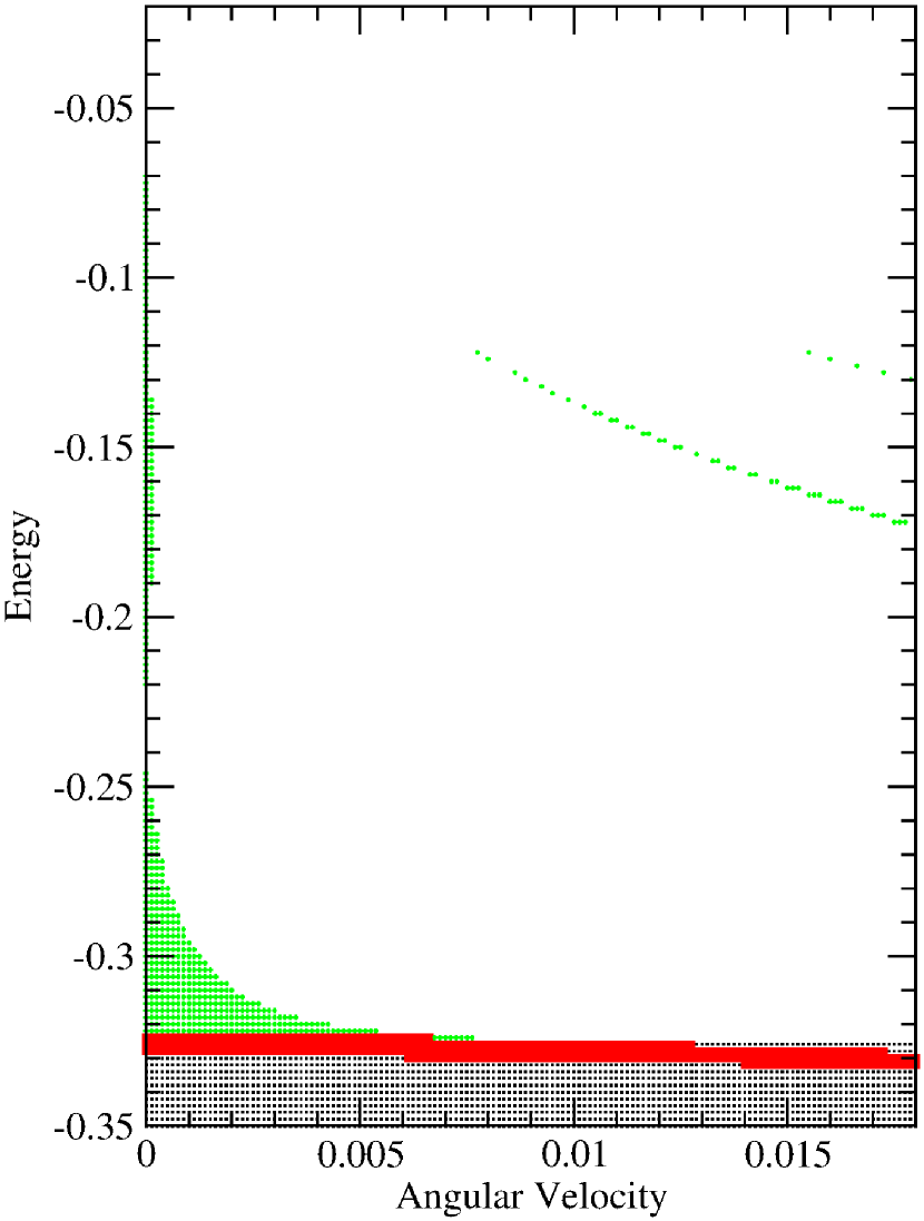
Figure 1: Types of orbits in the angular velocity vs. energy diagram. Orbits with null Lyapunov exponents are shown as dots (black in the electronic version) and orbits with only one positive Lyapunov exponent as filled squares (red in the electronic version). The blank space corresponds to orbits with two equal non-zero Lyapunov exponents and plus signs (green in the electronic version) represent orbits with two non-zero Lyapunov exponents that are not equal.

Fig. 1 presents our results and it can be compared with Figure 2 of Patsis & Zachilas (1990). The stable and simply unstable regions of their diagram agree very well with the regions of our Fig. 1 that correspond, respectively, to our regions with all null and with just one positive Lyapunov exponents. The comparison of the doubly unstable and complex unstable regions of Patsis and Zachilas with our regions occupied by orbits with two positive Lyapunov exponents and, respectively, $\lambda_{1}\neq\lambda_{2}$ and $\lambda_{1}=\lambda_{2}$ shows, however, some small disagreements. For a rotationless galaxy our results give orbits with $\lambda_{1}=\lambda_{2}>0$ for energies between $-0.245$ and $-0.220$ as well as for energies larger than $-0.070$, although the results of Patsis and Zachilas give doubly unstable orbits for all energies. Besides, the two lanes of orbits with two positive Lyapunov exponents and $\lambda_{1}\neq\lambda_{2}$ in the upper right region of our figure do not extend to energies larger than $-0.120$, while the corresponding lanes of doubly unstable orbits of Patsis and Zachilas continue up to the top of their figure. The problem is that the differences between $\lambda_{1}$ and $\lambda_{2}$ are very small in those regions and close to the precision of our computations. The differences between the two positive Lyapunov exponents of the orbits in the uppermost right lane, for example, are about $1.50\times 10^{-4}$, i.e. very near our limiting value of $1.25\times 10^{-4}$. The method of the monodromy matrix seems, therefore, to be better than Lyapunov exponents to distinguish doubly unstable from complex unstable periodic orbits, but that is not a problem for us because we did not intend to replace the method of the monodromy matrix by the use of Lyapunov exponents.

4 Conclusions

We have proven that stable periodic orbits have null Lyapunov exponents, simply unstable periodic orbits have only one positive Lyapunov exponent, doubly unstable periodic orbits have two different positive Lyapunov exponents and complex unstable periodic orbits have two equal positive Lyapunov exponents. A corollary of our result is that complex instability does not exist in systems with two-dimensional (2D) configuration spaces, an assertion that Contopoulos (2002, p. 287) gives without proof, because complex instability demands an exponential expansion in two dimensions but only one is available in 2D autonomous systems (the other one has a zero Lyapunov exponent).

The most important result of our study is that the stability of the periodic orbits (revealed by their Lyapunov exponents) drastically affects the phase space in their neighborhood and, as a result, stable, simply unstable and both doubly and complex unstable periodic orbits should be surrounded by families of, respectively, regular, partially and fully chaotic orbits. Thus, our result gives further support to the existence of partially chaotic orbits.

We have investigated the presence of chaos in many galactic models in the past and our experience is that $\lambda_{1}$ is usually much larger than $\lambda_{2}$ when both are not zero. Thus, it was surprising to find that almost 98 per cent of the orbits with two non-zero Lyapunov exponents in Figure 1 have $\lambda_{1}=\lambda_{2}$. The most likely explanation for this oddity is that all the orbits in that sample are periodic, while in our models it would have been almost impossible to find a periodic orbit by chance.

References

- Benettin et al. (1976) Benettin G., Galgani L., Strelcyn J.-M., 1976, Phys. Rev. A, 14, 2338
- Benettin et al. (1980) Benettin G., Galgani L., Giorgilli A., Strelcyn J.-M., 1980, Meccanica, 15, 9
- Berglund (2001) Berglund N., 2001, arXiv Mathematics e-prints, p. math/0111177
- Binney & Tremaine (2008) Binney J., Tremaine S., 2008, Galactic Dynamics: (Second Edition). Princeton Series in Astrophysics, Princeton University Press, http://books.google.com.ar/books?id=qxWt20TH--cC
- Carpintero & Muzzio (2016) Carpintero D. D., Muzzio J. C., 2016, MNRAS, 459, 1082
- Carpintero et al. (2014) Carpintero D. D., Muzzio J. C., Navone H. D., 2014, MNRAS, 438, 2871
- Contopoulos (2002) Contopoulos G., 2002, Order and chaos in dynamical astronomy
- Contopoulos & Magnenat (1985) Contopoulos G., Magnenat P., 1985, Celestial Mechanics, 37, 387
- Contopoulos et al. (1978) Contopoulos G., Galgani L., Giorgilli A., 1978, Phys. Rev. A, 18, 1183
- Floquet (1883) Floquet G., 1883, Annales de l’École Normale Supérieure, 12, 47
- Froeschlé (1970) Froeschlé C., 1970, A&A, 4, 115
- Froeschlé (1971) Froeschlé C., 1971, Ap&SS, 14, 110
- Guckenheimer & Holmes (2013) Guckenheimer J., Holmes P., 2013, Nonlinear Oscillations, Dynamical Systems, and Bifurcations of Vector Fields. Applied Mathematical Sciences, Springer New York, https://books.google.com.ar/books?id=XYIpBAAAQBAJ
- Hadjidemetriou (1975) Hadjidemetriou J. D., 1975, Celestial Mechanics, 12, 255
- Lichtenberg & Lieberman (1992) Lichtenberg A., Lieberman M., 1992, Regular and Chaotic Dynamics
- Magnenat (1982) Magnenat P., 1982, Celestial Mechanics, 28, 319
- Miyamoto & Nagai (1975) Miyamoto M., Nagai R., 1975, PASJ, 27, 533
- Muzzio (2006) Muzzio J. C., 2006, Celestial Mechanics and Dynamical Astronomy, 96, 85
- Muzzio (2017) Muzzio J. C., 2017, MNRAS, 471, 4099
- Muzzio (2018) Muzzio J. C., 2018, MNRAS, 473, 4636
- Muzzio et al. (2005) Muzzio J. C., Carpintero D. D., Wachlin F. C., 2005, Celest. Mech. Dynam. Astron., 91, 173
- Muzzio et al. (2009) Muzzio J. C., Navone H. D., Zorzi A. F., 2009, Celest. Mech. Dynam. Astron., 105, 379
- Patsis & Zachilas (1990) Patsis P. A., Zachilas L., 1990, A&A, 227, 37
- Patsis & Zachilas (1994) Patsis P. A., Zachilas L., 1994, International Journal of Bifurcation and Chaos, 6, 1399
- Pettini & Vulpiani (1984) Pettini M., Vulpiani A., 1984, Physics Letters A, 106, 207
- Roxin & Spinadel (1976) Roxin E. O., Spinadel V. W., 1976, Ecuaciones diferenciales parciales, 2nd edn. Editorial Universitaria de Buenos Aires
- Udry & Pfenniger (1988) Udry S., Pfenniger D., 1988, A&A, 198, 135
- Wiggins (1990) Wiggins S., 1990, Introduction to Applied Nonlinear Dynamical Systems and Chaos. Springer, https://ci.nii.ac.jp/naid/10007477604/en/
- Zorzi & Muzzio (2012) Zorzi A. F., Muzzio J. C., 2012, MNRAS, 423, 1955