Fractional norms and quasinorms do not help to overcome the curse of dimensionality

Abstract

The curse of dimensionality causes the well-known and widely discussed problems for machine learning methods. There is a hypothesis that using of the Manhattan distance and even fractional quasinorms lp (for p less than 1) can help to overcome the curse of dimensionality in classification problems. In this study, we systematically test this hypothesis. We confirm that fractional quasinorms have a greater relative contrast or coefficient of variation than the Euclidean norm l2, but we also demonstrate that the distance concentration shows qualitatively the same behaviour for all tested norms and quasinorms and the difference between them decays as dimension tends to infinity. Estimation of classification quality for kNN based on different norms and quasinorms shows that a greater relative contrast does not mean better classifier performance and the worst performance for different databases was shown by different norms (quasinorms). A systematic comparison shows that the difference of the performance of kNN based on lp for p=2, 1, and 0.5 is statistically insignificant.

I Introduction

The term “curse of dimensionality” was introduced by Bellman [1]. Nowadays, this is a general term for problems related to high dimensional data, for example, for Bayesian modelling [2], nearest neighbour prediction [3] and search [4], neural networks [5], and many others. Many authors [6], [7], [8], [9], [10] studied the “meaningfulness” of distance based classification in high dimensions. These studies are related to the distance concentration, which means that in high dimensional space the distances between almost all pairs of points have almost the same value.

The term “blessing of dimensionality” was introduced by Kainen in 1997 [11]. The “blessing of dimensionality” considers the same distance concentration effect from the different point of view [12], [13], [14], [15], [16]. The distance concentration was discovered in the foundation of statistical physics and analysed further in the context of probability theory, functional analysis, and geometry (reviewed by [17], [14], [18], [19]). The blessing of dimensionality allows us to use some specific high dimensional properties to solve problems [20],[21]. The important property is linear separability of points from random sets in high dimensions [14], [16].

The $l_{p}$ functional $\|x\|_{p}$ in $d$ dimensional vector space is defined as

$$\|x\|_{p}=\left(\sum_{i=1}^{d}x_{i}^{p}\right)^{1/p}.$$ (1)

It is a norm for $p\geq 1$ and a quasinorm for $0<p<1$ because of violation of the triangle inequality [22]. It is well known that for $p<q$ we have $\|x\|_{p}\geq\|x\|_{q},\forall x$.

Measurement of dissimilarity and errors by subquadratic functionals reduces the effect of outliers and can help to construct more robust data analysis methods [23], [8], [19]. Utilisation of these functionals for struggling with the curse of dimensionality was proposed in several works [8], [19], [24], [25] [26], [27].

In 2001, C.C. Aggarwal with co-authors [8] described briefly the effect of using fractional quasinorms for high-dimensional problems. They demonstrated that using of $l_{p}$ ($p\leq 1$) can compensate the distance concentration. This idea was used further in many works [28], [29], [10]. One of the main problems of $l_{p}$ quasinorms usage for $p<1$ is time of calculation of minimal distances and solution of optimization problems with $l_{p}$ functional (which a even non-convex for $p<1$). Several methods have been developed to accelerate the calculations [28], [30]. The main outcome of [8] was the use of Manhattan distance instead of Euclidean one [31], [32], [33]. The main reason for this is the fact that for $p<1$ functional $l_{p}$ is not a norm but is a non-convex quasinorm. All methods and algorithms which assume triangle inequality [32], [34], [35] cannot use such a quasinorm.

Comparison of different $l_{p}$ functionals for data mining problems is yet fragmental, see, for example, [8], [36], [37]. In our study, we performed systematic testing. In general case distance concentration for $l_{p}$ functionals was less for lower $p$ but for all $p$ the shape of distance concentration as a function of dimension is qualitatively the same. Moreover, the difference in distance concentration for different $p$ decreases with dimension increasing. We systematically tested the hypothesis that the measurement of dissimilarity by subquadratic norms $l_{p}(1\leq p<2)$ or even quasinorms $(0<p<1)$ can help to overcome the curse of dimensionality in classification problems. We demonstrated that these norms and quasinorms do not improve k Nearest Neighbour (kNN) classifiers in high dimensions systematically and significantly.

There are two main results in this study: (i) usage of $l_{p}$ functionals with small $p$ does not prevent the distance concentration and (ii) the smaller distance concentration does not mean the better accuracy of kNN classification.

The further part of our paper is organised as follows. In Section ‘Measure concentration’ we presented results of an empirical test of distance concentration for Relative Contrast (RC) and Coefficient of Variation (CV) also known as relative variance. In Section ‘Dimension estimation’ we presented description of 6 used dimensions. In Section ‘Comparison of $l_{p}$ functionals’ we describe the approaches used for $l_{p}$ functionals comparison, the used databases and the classification quality measures. In Section ‘Dimension comparison’ we presented results of 6 discussed dimensions comparison. In Section ‘Results of $l_{p}$ functionals comparison’ we presented results of the described tests to compare different $l_{p}$ functionals. In Section ‘Discussion’ discussion and outlook are presented.

All software and databases used for this study can be found in [38]. Some results of this work were presented partially at IJCNN2019 [39].

II Measure concentration

Let us consider a database $X$ with $n$ data points $X={x_{1},\ldots,x_{n}}$ and $d$ real-valued attributes, $x_{i}=(x_{i1},\ldots,x_{id})$. We consider databases of two types: randomly generated database with i.i.d. components from the uniform distribution on the interval $[0,1]$ (this section) and real life databases (Section IV). The $l_{p}$ functional for vector $x$ is defined by (1). For comparability of results in this study we consider set of norms and quasinorms used in [8] with one more quasinorm ($l_{0.01}$): $l_{0.01},l_{0.1},l_{0.5},l_{1},l_{2},l_{4},l_{10},l_{\infty}$.

Fig. 1 shows forms of unit level sets for all considered norms and quasinorms excluding $l_{0.01}$ and $l_{0.1}$. For these two quasinorms, graphs are visually indistinguishable from the central cross.

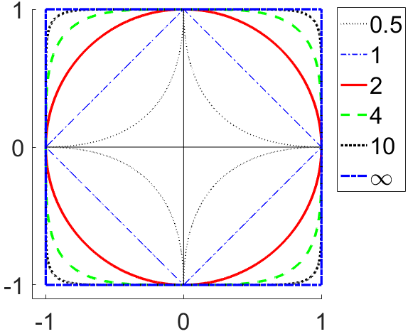
Figure 1: Unit level sets for $l_{p}$ functionals (“Unit spheres”).

Several different indicators were used to study distance concentration:

• Relative Contrast (RC) [6], [8], [19]

  $$\text{RC}_{p}(X,y)=\frac{|\max_{i}\|x_{i}-y\|_{p}-\min_{i}\|x_{i}-y\|_{p}|}{\min_{i}\|x_{i}-y\|_{p}};$$ (2)

• Coefficient of Variations (CV) or relative variance [34], [35], [19]

  $$\text{CV}_{p}(X,y)=\frac{\sqrt{var(\|x_{i}-y\|_{p}|)}}{mean(\|x_{i}-y\|_{p})},$$ (3)

  where $var(x)$ is variance and $mean(x)$ is mean value of random variable $x$;

• Hubness (popular nearest neighbours) [10].

In our study we use RC and CV.

Table 2 in [8] shows that fraction of cases where $\text{RC}_{1}>\text{RC}_{2}$ increases with dimension. It can be easily shown that for specific choice of $X$ and $y$ all three relations between RC₁ and RC₂ are possible $\text{RC}_{1}(X,y)>\text{RC}_{2}(X,y)$, $\text{RC}_{1}(X,y)=\text{RC}_{2}(X,y)$, or $\text{RC}_{1}(X,y)<\text{RC}_{2}(X,y)$. To evaluate the probabilities of these three outcomes, we performed the following experiment. We generated dataset $X$ with $k$ points and $100$ coordinates. Each coordinate of each point was uniformly randomly generated for the interval $[0,1]$. For each dimension $d=1,2,3,4,10,15,20,100$ we create $d$ dimensional database $X_{d}$ by selection of the first $d$ coordinates of points in $X$. We calculated $\text{RC}_{p}$ as the mean value of RC for each point of $X_{d}$:

$$\text{RC}_{p}=\frac{1}{k}\sum_{i=1}^{k}\text{RC}_{p}(X_{d}\backslash\{x_{i}\},x_{i}),$$

where $X\backslash\{y\}$ is the database $X$ without point $y$. We repeated this procedure 1000 times and calculated the fraction of cases when $\text{RC}_{1}(X,y)>\text{RC}_{2}(X,y)$. Results of this experiment are presented in Table I. Table I shows that for $k=10$ points our results are very similar to the results presented in Table 2 in [8]. Increasing of number of points shows that already for relatively small number of points ($k\approx 20$) for almost all databases $\text{RC}_{1}(X,y)>\text{RC}_{2}(X,y)$.

TABLE I: Comparison of RC for $l_{1}$ and $l_{2}$ for different dimension (Dim) and different number of points

Dim	$P(\text{RC}_{2}<\text{RC}_{1})$ for # of points
	10 [8]	10	20	100
1	0	0	0	0
2	0.850	0.850	0.960	1.00
3	0.887	0.930	0.996	1.00
4	0.913	0.973	0.996	1.00
10	0.956	0.994	1.00	1.00
15	0.961	1.000	1.00	1.00
20	0.971	0.999	1.00	1.00
100	0.982	1.000	1.00	1.00

This means that appearance of non-negligible fraction of cases where $\text{RC}_{2}>\text{RC}_{1}$ is caused by very small size of a sample. For not so small samples we almost always have $\text{RC}_{2}<\text{RC}_{1}$. The main reason for this is different pairs of closest and furthest points for different metrics. Several examples of such sets are presented in Fig. 2. Fig. 2 shows that $\text{RC}_{2}<\text{RC}_{\infty}$ in rows 3, 5, 6, and 8 and $\text{RC}_{1}<\text{RC}_{2}$ in row 6. These results allows us to formulate a hypothesis that in general case almost always $\text{RC}_{p}<\text{RC}_{q},\forall p>q$. RC widely used to study properties of finite set of points but for distributions of points the CV is more appropriate. We assume that for CV hypothesis $\text{CV}_{p}<\text{CV}_{q},\forall p>q$ is also true.

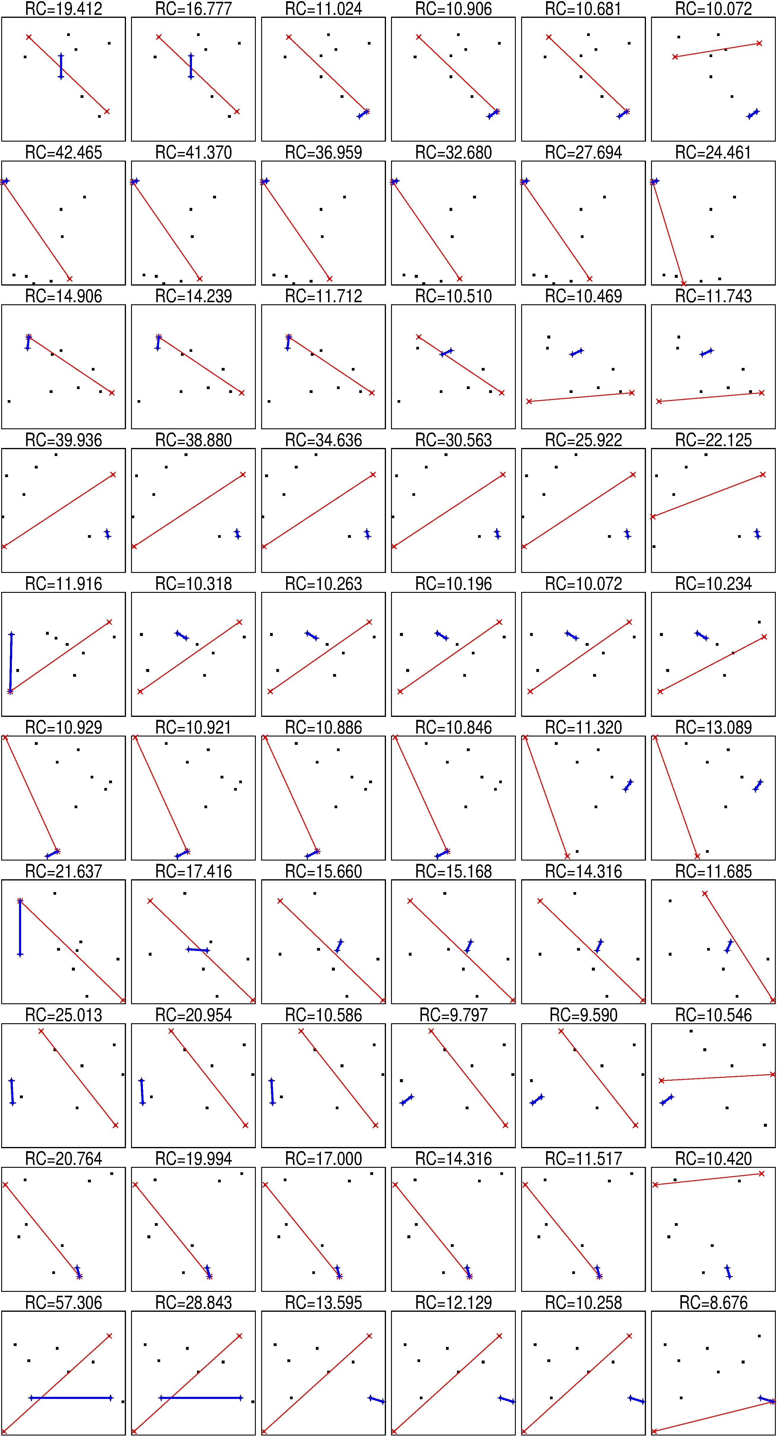
Figure 2: 10 randomly generated sets of 10 points, thin red line connects the furthest points and bold blue line connects closest points, columns (from left to right) corresponds to $p=0.01,0.1,0.5,1,2,\infty$

To check this hypothesis we performed the following experiment. We generated database $X$ with 10,000 points in 200 dimensional space. Each coordinate of each point was uniformly randomly generated for the interval $[0,1]$. We selected the set of dimensions $d=1,2,3,4,5,10,15,\ldots,195,200$ and the set of $l_{p}$ functionals $l_{0.01},l_{0.1},l_{0.5},l_{1},l_{2},l_{4},l_{10},l_{\infty}$. For each dimension $d$ we prepared the database $X_{d}$ as the set of the first $d$ coordinates of points in database $X$. For each database $X_{d}$ and $l_{p}$ functional we calculate the set of all pairwise distances $D_{dp}$. Then we estimated the following values:

$$\text{RC}_{p}=\frac{\max D_{dp}-\min D_{dp}}{\min D_{dp}},\text{CV}_{p}=\frac{\sqrt{var(D_{dp})}}{mean(D_{dp})}.$$

Graphs of $\text{RC}_{p}$ and $\text{CV}_{p}$ are presented in Fig. 3. Fig. 3 shows that our hypotheses are true. We can see that RC and CV as functions of dimension have qualitatively the same shape but in different scales: RC in the logarithmic scale. The paper [8] states that qualitatively different behaviour of $\max_{i}\|x_{i}\|_{p}-\max_{i}\|x_{i}\|_{p}$ for different $p$. We can state that for relative values we observe qualitatively the same behaviour with small quantitative difference $\text{RC}_{p}-\text{RC}_{q}$ which decreases with dimensionality increasing. This means that that there could be some preference in usage of lower values of $p$ but the fractional metrics do not provide a panacea from the curse of dimensionality. To analyse this hypothesis, we study the real live benchmarks in the next section.

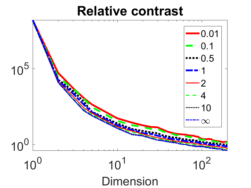
Figure 3: Changes of RC (left) and CV (right) with dimension increasing for several metrics

III Dimension estimation

To consider high dimensional data and curse or blessing of dimensionality, it is necessary to determine what a dimension is. There are many different notions of dimension. Evaluation of dimension become very important with appearing of many “big data” databases. The number of attributes is dimension of vector space or Hamel dimension [40] (denoted further as #Attr). Fortunately, for the data mining problems the space dimension is not so important as a data dimension. Intrinsic or effective dimension of data is not so well defined term by an obvious reason: the datasets are finite and, therefore, the direct application of the topological definitions of dimension gives zero. The most popular approach to definition of data dimension is approximation of data sets by a continuous topological object. Perhaps, the first and, at the same time, the widely used definition of intrinsic dimension is the dimension of linear manifold of “the best fit to data” with sufficiently small deviations [41]. The simplest way to calculate such dimension is Principle Component Analysis (PCA) [42]. Unfortunately there is no unique methods to define number of informative (important, relevant, etc.) PCs [43], [44], [45]. Two most widely used methods are Kaiser rule [46] (denoted further as PCA-K), [47] and Broken stick rule [43] (denoted further as PCA-BS).

Let us consider a database $X$ with $n$ data points $X={x_{1},\ldots,x_{n}}$ and $d$ real-valued attributes, $x_{i}=(x_{i1},\ldots,x_{id})$. Principal components correspond to eigenvalues of empirical covariance matrix $\Sigma(X)=X^{T}X$. This matrix is symmetric and non-negative defined. This means that eigenvalues of $\Sigma(X)$ matrix are non-negative real numbers. Let us denote these values as $\lambda_{1}\geq\lambda_{2}\geq\cdots\geq\lambda_{d}$. Fraction of Variance Explained (FVE) by $i$ PC is $f_{i}=\frac{\lambda_{i}}{\sum_{j=1}^{d}\lambda_{j}}$.

Kaiser rule states that all PC with FVE greater or equal to average FVE ($1/d$) are informative.

Let us consider unit interval (stick) randomly broken into $d$ fragments. Let us numerate this fragments with decreasing of their length: $s_{1}\geq s_{2}\geq\cdots\geq s_{d}$. Expected length of $i$ fragment is

$$b_{i}=\frac{1}{d}\sum_{j=i}^{d}\frac{1}{j}.$$ (4)

Broken stick rule states that the first $k$ PCs are informative, where $k$ is the maximal number such that $f_{i}\geq b_{i},\forall i\leq k$.

In many problems empirical covariance matrix degenerates. Let us consider projection of data onto the first $k$ PCs: $\hat{X}=XV$, where columns of matrix $V$ are the first $k$ eigenvectors of $\Sigma(X)$ matrix. Eigenvalues of the empirical covariance matrix $\Sigma(\hat{(}X))$ are $\lambda_{1},\lambda_{2},\ldots,\lambda_{k}$. After dimensionality reduction the condition number of the reduced covariance matrix should not be high in order to avoid the multicollinearity problems. The relevant definition [16] of the intrinsic dimensionality refers directly to the conditional number of $\Sigma(X)$ matrix: $k$ is the number of the informative PCs if it is the smallest number such that

$$\frac{\lambda_{k+1}}{\lambda_{1}}<\frac{1}{C},$$ (5)

where C is specified conditional number, for example $C=10$. This approach is referred further as PCA-CN. The PCA-CN intrinsic dimensionality is defined as the number of eigenvalues of the covariance matrix that exceed a fixed percent of its largest eigenvalue [48].

Development of the idea of data approximation led to Principal Manifolds [49] and more sophisticated approximators like Principal graphs and complexes [50], [51]. These approaches provide tools for evaluating the intrinsic dimensionality of data and measuring the data complexity [52]. Another approach uses the complexes with vertices in data points: just connect the points with distance less than $\varepsilon$ for variable $\varepsilon$ and receive an object of combinatorial topology, a simplicial complex [53]. All these methods use an object embedded into a dataspace. They are called Injective Methods [54]. Additionally, a family of Projective Methods was developed. They do not construct an approximator but project the dataspace on a lower dimensional space with preservation of objects similarity or dissimilarity. For a brief review of modern injective and projective methods we refer to [54].

Recent development of curse/blessing dimensionality studies introduce new method of intrinsic dimension evaluation separability analysis. Detailed description of this method can be found in [16] and [55] (denoted further as SepD). For this study we used implementation of separability analysis from the [56]. The main notion of this approach is $\alpha$ Fisher separability: point $x$ of dataset $X$ is $\alpha$ Fisher separable from dataset $X$ if

$$(x,y)\leq\alpha(x,x),\forall y\in X,y\neq x,$$ (6)

where $(x,y)$ is dot product of vectors $x$ and $y$.

The last used in this study intrinsic dimension is fractal dimension (denoted further as FracD). There are many versions of fractal dimension and we used R implementation from the RDimtools package [57]. The considered definition of a fractal dimension is

$$d_{f}=\lim_{r\to 0}\frac{\log(N(r))}{\log(1/r)},$$

where $r$ is the $d$-cubic box size in the regular grid and $N(r)$ is number of cells with data points in this grid. Since we work with the finite dataset the limit is substituted by slope of linear regression without intercept.

IV Comparison of $l_{p}$ functionals

In Section II, we demonstrated that $\text{RC}_{p}$ is higher for smaller $p$. Paper [6] shows that greater RC means ‘more meaningful’ task for kNN. We decide to compare different $l_{p}$ functions for kNN classification. Classification has one additional benefit in comparison with regression and clustering problems: classification quality measure is classifier independent and similarity measure independent [58]. For this study we selected three classification quality measures: Total Number of neighbours of the Same Class (TNNSC), accuracy (fraction of correctly recognised cases), sum of sensitivity (fraction of correctly solved cases of positive class) and specificity (fraction of correctly solved cases of negative class). TNNSC is not an obvious measure of classification quality and we use it for comparability of our results with [8]. The 11 nearest neighbours as the method of classification was selected also for comparability with [8].

IV-A Databases for comparison

We selected 25 databases from UCI data repository [59]. We applied the following criteria for the database selection:

1. Data are not time-series.

2. Database is formed for the binary classification problem.

3. Database does not contain any missed values.

4. Number of attributes is less than number of observations and is greater than 3.

5. All predictors are binary or numeric.

Totally, we selected 25 databases and 37 binary classification problems. For simplicity further we call each problem a ‘database’. The list of selected databases is presented in Table II.

TABLE II: Databases selected for analysis

Name	Source	#Attr.	Cases	PCA-K	PCA-BS	PCA-CN	SepD	FracD
Blood	[60]	4	748	2	2	3	2.4	1.6
Banknote authentication	[61]	4	1,372	2	2	3	2.6	1.9
Cryotherapy	[62], [63], [64]	6	90	3	0	6	4.1	2.5
Vertebral Column	[65]	6	310	2	1	5	4.4	2.3
Immunotherapy	[62], [63], [66]	7	90	3	0	7	5.1	3.2
HTRU2	[67], [68], [69]	8	17,898	2	2	4	3.06	2.4
ILPD (Indian Liver
Patient Dataset)	[70]	10	579	4	0	7	4.3	2.1
Planning Relax	[71]	10	182	4	0	6	6.09	3.6
MAGIC Gamma Telescope	[72]	10	19,020	3	1	6	4.6	2.9
EEG Eye State	[73]	14	14,980	4	4	5	2.1	1.2
Climate Model Simulation
Crashes	[74]	18	540	10	0	18	16.8	21.7
Diabetic Retinopathy Debrecen	[75], [76]	19	1,151	5	3	8	4.3	2.3
SPECT Heart	[77]	22	267	7	3	12	4.9	11.5
Breast Cancer	[78]	30	569	6	3	5	4.3	3.5
Ionosphere	[79]	34	351	8	4	9	3.9	3.5
QSAR biodegradation	[80], [81]	41	1,055	11	6	15	5.4	3.1
SPECTF Heart	[77]	44	267	10	3	6	5.6	7
MiniBooNE particle
identification	[82]	50	130,064	4	1	1	0.5	2.7
First-order theorem proving
(6 tasks)	[83], [84]	51	6,118	13	7	9	3.4	2.04
Connectionist Bench (Sonar)	[85]	60	208	13	6	11	6.1	5.5
Quality Assessment of
Digital Colposcopies (7 tasks)	[86], [87]	62	287	11	6	9	5.6	4.7
LFW	[88]	128	13,233	51	55	57	13.8	19.3
Musk 1	[89]	166	476	23	9	7	4.1	4.4
Musk 2	[89]	166	6,598	25	13	6	4.1	7.8
Madelon	[90], [91]	500	2,600	224	0	362	436.3	13.5
Gisette	[92], [90]	5,000	7,000	1465	133	25	10.2	2.04

We do not try to identify the best database preprocessing for each database. We simply use three preprocessing for each database:

• empty preprocessing means usage data ‘as is’;

• standardisation means to shift and scale data to have zero mean and unit variance;

• min-max normalization means to shift and scale data to belong interval $[0,1]$.

IV-B Approaches to comparison

Our purpose is to compare metrics but not to create the best classifier to solve each problem. Following [1] we use 11NN classifier. One of the reasons to select kNN is strong dependence of kNN on selected metrics and, on the other hand, the absence of any assumption about data, excluding the principle: tell me your neighbours, and will I tell you what you are. In our study we consider 11NN with $l_{0.01},l_{0.1},l_{0.5},l_{1},l_{2},l_{4},l_{10},l_{\infty}$ as different algorithms. We applied the following indicators to compare 11NN classifiers (algorithms) for listed $l_{p}$ functionals:

• number of databases for which algorithm is the best [93];

• number of databases for which algorithm is the worst [93];

• number of databases for which algorithm has performance which statistically insignificantly different from the best;

• number of databases for which algorithm has performance which statistically insignificantly different from the worst;

• Friedman test [94], [95] and post hoc Nomenyi test [96] which were specially developed for multiple algorithms comparison;

• Wilcoxon signed rank test was used for comparison of three pairs of metrics.

The first four approaches we call frequency comparison. To avoid discrepancies, a description of all statistical tests used is presented below.

IV-B1 Proportion estimation

Since two measures of classification quality accuracy and $\text{TNNSC}/(11\times n)$, where $n$ is number of cases in database, are proportions we can apply z-test of proportion estimations [97]. We to compare two proportions with the same sample size, hence, we can use simplified formula for test statistics:

$$z=\frac{|p_{1}-p_{2}|}{\sqrt{\frac{p_{1}+p_{2}}{n}\big{(}1-\frac{p_{1}+p_{2}}{2}\big{)}}},$$

where $p_{1}$ and $p_{2}$ are two proportions to compare. P-value of this test is probability of observing by chance the same or greater $z$ if both samples are taken from the same population. P-value is $p_{z}=\Phi(-z)$, where $\Phi(z)$ is standard cumulative normal distribution. We also meet the problem of reasonable selection of significance level. Selected databases contain from 90 to 130,064 cases. Usage of the same threshold for all databases is meaningless [98], [99]. The necessary sample size $n$ can be estimated through the specified significance level of $1-\alpha$, the statistical power $1-\beta$, the expected effect size $e$, and the population variance $s^{2}$. For the normal distribution (since we use z-test):

$$n=\frac{2(z_{1-\alpha}+z_{1-\beta})^{2}s^{2}}{d^{2}}.$$

In this study, we assume that the significance level is equal to the statistical power $\alpha=\beta$, the expected effect size is 1% (1% difference in accuracy is big enough), and the population variance can be estimated by

$$s^{2}=n\frac{n_{+}}{n}\big{(}1-\frac{n_{+}}{n}\big{)}=\frac{n_{+}(n-n_{+})}{n},$$

where $n_{+}$ is number of cases in the positive class. Under this assumptions, we can estimate reasonable significance level as

$$\alpha=\Phi\left(\frac{d}{s}\sqrt{\frac{n}{8}}\right).$$

Usage of 8 $l_{p}$ functionals means multiple testing. To avoid overdetection problem we apply Bonferroni correction [100]. From the other side, usage of too big significance level is also meaningless [98]. As a result we select the significance level as

$$\alpha=\max\bigg{\{}\frac{1}{28}\Phi\bigg{(}\frac{d}{s}\sqrt{\frac{n}{8}}\bigg{)},0.00001\bigg{\}}.$$

Differences between two proportions (TNNSC or accuracies) is statistically significant if $p_{z}<\alpha$. It is necessary to stress that for TNNSC the number of cases is $11n$ because we consider 11 neighbours for each point.

IV-B2 Friedman test and post hoc Nomenyi test

One of the widely used statistical tests for algorithms comparison on many databases is Friedman test [94], [95]. To apply this test, we need firstly to apply tied ranking for the classification quality measure for one database: if several classifiers provide exactly the same quality measure then rank of all such classifiers will be equal to average value of the ranks for which they were tied [95]. Let us denote the number of used databases as $N$, the number of used classifiers as $m$ and the rank of classifier $i$ for database $j$ as $r_{ji}$. Mean rank of classifier $i$ is

$$R_{i}=\frac{1}{N}\sum_{j=1}^{N}r_{ji}.$$

Test statistics is

$$\chi^{2}_{F}=\frac{4N^{2}(m-1)\Big{(}\sum_{i=1}^{m}R_{i}^{2}-\frac{m(m+1)^{2}}{4}\Big{)}}{4\sum_{i=1}^{m}\sum_{j=1}^{N}r_{ji}^{2}-Nm(m+1)^{2}}.$$

Test statistics under null hypothesis that all classifiers have the same performance follows $\chi^{2}$ distribution with $m-1$ degrees of freedom. P-value of this test is probability of observing by chance the same or greater $\chi^{2}_{F}$ if all classifiers have the same performance. P-value is $p_{\chi}=1-F(\chi^{2}_{F};m-1)$, where $F(\chi;df)$ is cumulative $\chi^{2}$ distribution with $df$ degrees of freedom. Since we have 37 databases only we decide to use 95% significance level.

If Friedman test shows enough evidence to reject null hypothesis then we can conclude that not all classifiers have the same performance. To identify the pairs of classifiers with significantly different performance we applied post hoc Nomenyi test [96]. Test statistics for comparison of $i$ and $j$ classifiers is $|R_{i}-R_{j}|$. To identify pairs with statistically significant differences the critical distance

$$\text{CD}=q_{\alpha m}\sqrt{\frac{m(m+1)}{6N}}.$$

is used. $q_{\alpha m}$ is critical value for Nomenyi test with significance level of $1-\alpha$ and $m$ degrees of freedom. The difference of classifiers performances is statistically significant with significance level of $1-\alpha$ if $|R_{i}-R_{j}|>CD$.

IV-B3 Wilcoxon signed rank test

To compare the performance of two classifiers on several databases we applied Wilcoxon signed rank test [101]. For this test we used standard Matlab function signrank [102].

V Dimension comparison

We can see in Table II that for all definitions of intrinsic dimension of data this dimension does not grow monotonically with the number of attributes for the given set of benchmarks. The correlation matrix of all six dimensions is presented in Table III. There are two groups of highly correlated:

• #Attr, PCA-K and PCA-BS;

• PCA-CN and SepD.

The correlations between groups are low (maximal value 0.154). The last dimension - FracD - is correlated (but not strongly correlated) with PCA-CN and SepD.

TABLE III: Correlation matrix for six dimensions: two groups of highly correlated estimates are highlighted by background

Dimension	#Attr	PCA-K	PCA-BS	PCA-CN	SepD	FracD
#Attr	1.000	0.998	0.923	0.098	0.065	-0.081
PCA-K	0.998	1.000	0.917	0.154	0.119	-0.057
PCA-BS	0.923	0.917	1.000	0.018	-0.058	0.075
PCA-CN	0.098	0.154	0.018	1.000	0.992	0.405
SepD	0.065	0.119	-0.058	0.992	1.000	0.343
FracD	-0.081	-0.057	0.075	0.405	0.343	1.000

Let us consider the first group of correlated dimensions. Linear regressions PCA-K and PCA-BS of #Attr are

$$\begin{split}\text{PCA-K}&=0.29\text{\#Attr},\\ \text{PCA-BS}&=0.027\text{\#Attr}.\end{split}$$

It is necessary to emphasize that coefficient 0.29 (0.027 for PCA-BS) was defined for datasets considered in this study only and can be different for another datasets but multiple R squared equals 0.998 (0.855 for PCA-BS) shows that this dependence is not occasional. What is a reason of so strong correlations of these dimensions. It can be shown that these dimensions are sensitive to irrelevant or redundant features. The simplest example is adding of highly correlated attributes. To illustrate this property of considered dimensions let us consider abstract database $X$ with $d$ standardised attributes and covariance matrix $\Sigma$. This covariance matrix has $d$ eigenvalues $\lambda_{1}\geq\lambda_{2}\geq\ldots\geq\lambda_{d}$ and corresponding eigenvectors $v_{1},\ldots,v_{d}$. To define PCA-K dimension we have to compare FVE of each PC with threshold $1/d$. Since all attributes are standardised we have unit values in the main diagonal of matrix $\Sigma$. This mean that $\sum_{i=1}^{d}\lambda_{i}=d$ and FVE of $i$ PC is $f_{i}=\frac{\lambda_{i}}{\sum_{j=1}^{d}\lambda_{j}}=\lambda_{i}/d$.

Consider duplication of attributes: add to the data table new attributes which are copies of the original attributes. This operation does not add any information to the data and, in principle, should not affect the internal dimension of the data for any reasonable definition.

Let us denote all object for this new database by $(1)$ in the superscript. New dataset can be denoted as $X^{(1)}=X|X$ where symbol $|$ denotes concatenation of two row vectors. For any data vectors $x^{(1)}$ and $y^{(1)}$ the dot product will be $(x^{(1)})^{\intercal}y^{(1)}=2x^{\intercal}y$, where $\intercal$ means matrix (vector) transpose.

For new dataset $X^{(1)}$ the covariance matrix has a form

$$\Sigma^{(1)}=\begin{bmatrix}\Sigma&\Sigma\\ \Sigma&\Sigma\end{bmatrix}.$$

The first $d$ eigenvectors can be presented in the form $v^{(1)}_{i}=(v_{i}^{\intercal}|v_{i}^{\intercal})^{\intercal}$. Now we can calculate product of $v^{(1)}_{i}$ and $\Sigma^{(1)}$:

$$\begin{split}\Sigma^{(1)}v^{(1)}_{i}=\begin{bmatrix}\Sigma&\Sigma\\ \Sigma&\Sigma\end{bmatrix}\begin{pmatrix}v_{i}\\ v_{i}\end{pmatrix}&=\begin{pmatrix}\Sigma v_{i}+\Sigma v_{i}\\ \Sigma v_{i}+\Sigma v_{i}\end{pmatrix}\\ =\begin{pmatrix}\lambda_{i}v_{i}+\lambda_{i}v_{i}\\ \lambda_{i}v_{i}+\lambda_{i}v_{i}\end{pmatrix}&=2\lambda_{i}\begin{pmatrix}v_{i}\\ v_{i}\end{pmatrix}=2\lambda_{i}v_{i}^{(1)}.\end{split}$$

As we can see each of the first $d$ eigenvalues become twice greater ($\lambda^{(1)}_{i}=2\lambda_{i},\forall i\leq d$). This means that FVE of the first $d$ PCs have the same values

$$f_{i}^{(1)}=\frac{\lambda^{(1)}_{i}}{2d}=\frac{2\lambda_{i}}{2d}=\frac{\lambda_{i}}{d}=f_{i},\forall i\leq d$$

Since sum of eigenvalues of matrix $\Sigma^{(1)}$ is $2d$ we can conclude that $\lambda^{(1)}_{i}=0,\forall i>d$. We can repeat described procedure several times and define values $\lambda^{(m)}_{i}=m\lambda_{i},f_{i}^{(m)}=f_{i}\forall i\leq d$ and $\lambda^{(m)}_{i}=0,\forall i>d$, where $m$ is number of adding copies of attributes. We need two more prepositions for broken stick. Let us have $d=2k$, then $b^{(1)}_{k+s}>b_{k+s},\forall s>0,b^{(1)}_{k-s}<b_{k-s},\forall s\geq 0$. Indeed, from (4):

$$\begin{split}b^{(1)}_{k+s}&=\frac{1}{4k}\sum_{j=k+s}^{4k}\frac{1}{j}\\ &=\frac{1}{4k}\Bigg{(}\sum_{j=k+s}^{2k}\frac{1}{j}+\sum_{j=k+1}^{2k}\frac{1}{2j}+\sum_{j=k+1}^{2k}\frac{1}{2j-1}\Bigg{)}\\ &>\frac{1}{4k}\Bigg{(}\sum_{j=k+s}^{2k}\frac{1}{j}+\sum_{j=k+1}^{2k}\frac{1}{2j}+\sum_{j=k+1}^{2k}\frac{1}{2j}\Bigg{)}\\ &=\frac{1}{4k}\Bigg{(}\sum_{j=k+s}^{2k}\frac{1}{j}+\frac{1}{2}\sum_{j=k+1}^{2k}\frac{1}{j}+\frac{1}{2}\sum_{j=k+1}^{2k}\frac{1}{j}\Bigg{)}\\ &=\frac{1}{2}\Bigg{(}\frac{1}{2k}\sum_{j=k+s}^{2k}\frac{1}{j}+\frac{1}{2k}\sum_{j=k+1}^{2k}\frac{1}{j}\Bigg{)}=\frac{1}{2}(b_{k+s}+b_{k+1})\\ &\geq\frac{1}{2}(b_{k+s}+b_{k+s})=b_{k+s}\end{split}$$

and

$$\begin{split}b^{(1)}_{k-s}&=\frac{1}{4k}\sum_{j=k-s}^{4k}\frac{1}{j}\\ &=\frac{1}{4k}\Bigg{(}\sum_{j=k-s}^{2k}\frac{1}{j}+\sum_{j=k+1}^{2k}\frac{1}{2j}+\sum_{j=k+1}^{2k}\frac{1}{2j-1}\Bigg{)}\\ &<\frac{1}{4k}\Bigg{(}\sum_{j=k-s}^{2k}\frac{1}{j}+\sum_{j=k+1}^{2k}\frac{1}{2j}+\sum_{j=k+1}^{2k}\frac{1}{2j-2}\Bigg{)}\\ &=\frac{1}{4k}\Bigg{(}\sum_{j=k-s}^{2k}\frac{1}{j}+\sum_{j=k+1}^{2k}\frac{1}{2j}+\sum_{j=k+1}^{2k}\frac{1}{2j}-\frac{1}{4k}\Bigg{)}\\ &<\frac{1}{2}\Bigg{(}\frac{1}{2k}\sum_{j=k-s}^{2k}\frac{1}{j}+\frac{1}{2k}\sum_{j=k+1}^{2k}\frac{1}{j}\Bigg{)}\\ &=\frac{1}{2}(b_{k-s}+b_{k+1})\leq\frac{1}{2}(b_{k-s}+b_{k-s})=b_{k-s}\end{split}$$

For case where $d=2k+1$ we have $b^{(1)}_{k+s}>b_{k+s},\forall s>1,b^{(1)}_{k-s}<b_{k-s},\forall s\geq-1$. Indeed, from (4):

$$\begin{split}b^{(1)}_{k+s}&=\frac{1}{4k}\sum_{j=k+s}^{4k+2}\frac{1}{j}\\ &=\frac{1}{4k}\Bigg{(}\sum_{j=k+s}^{2k+1}\frac{1}{j}+\sum_{j=k+1}^{2k+1}\frac{1}{2j}+\sum_{j=k+2}^{2k+1}\frac{1}{2j-1}\Bigg{)}\\ &>\frac{1}{4k}\Bigg{(}\sum_{j=k+s}^{2k+1}\frac{1}{j}+\sum_{j=k+1}^{2k+1}\frac{1}{2j}+\sum_{j=k+2}^{2k+1}\frac{1}{2j}\Bigg{)}\\ &=\frac{1}{2}b_{k+s}+\frac{1}{4}b_{k+1}+\frac{1}{4}b_{k+2}\\ &>\frac{1}{2}b_{k+s}+\frac{1}{4}b_{k+s}+\frac{1}{4}b_{k+s}=b_{k+s}\end{split}$$

and

$$\begin{split}b^{(1)}_{k-s}&=\frac{1}{4k}\sum_{j=k-s}^{4k+2}\frac{1}{j}\\ &=\frac{1}{4k}\Bigg{(}\sum_{j=k-s}^{2k+1}\frac{1}{j}+\sum_{j=k+1}^{2k+1}\frac{1}{2j}+\sum_{j=k+2}^{2k+1}\frac{1}{2j-1}\Bigg{)}\\ &<\frac{1}{4k}\Bigg{(}\sum_{j=k-s}^{2k+1}\frac{1}{j}+\sum_{j=k+1}^{2k+1}\frac{1}{2j}+\sum_{j=k+2}^{2k+1}\frac{1}{2j-2}\Bigg{)}\\ &=\frac{1}{4k}\Bigg{(}\sum_{j=k-s}^{2k+1}\frac{1}{j}+\sum_{j=k+1}^{2k+1}\frac{1}{2j}+\sum_{j=k+1}^{2k}\frac{1}{2j}\Bigg{)}\\ &<\frac{1}{4k}\Bigg{(}\sum_{j=k-s}^{2k+1}\frac{1}{j}+\sum_{j=k+1}^{2k+1}\frac{1}{2j}+\sum_{j=k+1}^{2k+1}\frac{1}{2j}\Bigg{)}\\ &=\frac{1}{2}b_{k-s}+\frac{1}{2}b_{k+1}\leq b_{k-s}\end{split}$$

Now we are ready to evaluate the effect of duplication of attributes on the linear dimension estimate, bearing in mind that nothing should change for reasonable definitions.

• For the vector space dimension we have simple formula: $\text{\#Attr}^{(m)}=md$.

• For Kaiser rule dimension PCA-K we have different threshold and now all PCs with FVE greater than $1/md$ are significant. This means that for all PCs with nonzero eigenvalues we can take big enough $m$ to provide “informativeness” of this PCs. Threshold of significance decays linearly with $m$ increasing.

• For broken stick dimension PCA-BS we observe initially increasing of threshold for the last half of original PCs but then thresholds $b^{(m)}_{i}$ will decay with $m$ increasing for all $i\leq d$. This means that for all PCs with nonlinear eigenvalues we can take big enough $m$ to provide “informativeness” of this PCs. Thresholds of significance decays non-linearly with $m$ increasing. This slower than linear decay of thresholds provide less sensitivity to irrelevant attributes.

• For conditional number based dimension PCA-CN nothing changes with described procedure because of simultaneous multiplying of all eigenvalues by nonzero constant does not change fraction of eigenvalues in condition (5).

• For separability dimension adding of irrelevant features does not change anything because dot products of data points in the extended database are dot products of original dataset multiplied by $m$. This means that described extension of dataset change nothing in the separability (6).

• There are no changes for the fractal dimension because of described extension of dataset do not change relative location of data points in space. This means that values $N(r)$ will be the same for original and extended datasets.

The second group of correlated dimensions includes PCA-CN, SepD, and FracD. The first two are extremely correlated and the last is moderately correlated with the first two. Linear regressions of these dimensions are

$$\begin{split}\text{SepD}&=1.17\text{PCA-CN},\\ \text{FracD}&=0.052\text{PCA-CN}.\end{split}$$

High correlation of these three dimensions requires additional investigations.

VI Results of $l_{p}$ functionals comparison

Results of frequency comparison are presented in Table IV. Table IV shows that indicator ‘The best’ is not robust and cannot be considered as a good tool for performance comparison [93]. For example, for TNNSC with empty preprocessing $l_{0.1}$ is the best for 11 databases and it is maximal value but $l_{0.5},l_{1}$ and $l_{2}$ are essentially better if we consider indicator ‘Insignificantly different from the best’: 26 databases for $l_{0.1}$ and 31 databases for $l_{0.5},l_{1}$ and $l_{2}$. Unfortunately we cannot estimate this indicator for ‘sensitivity plus specificity’ quality measure by used way (it can be done by t-test). Analysis of Table IV shows that in average $l_{0.5},l_{1},l_{2}$ and $l_{4}$ are the best and $l_{0.01}$ and $l_{\infty}$ are the worst. Results of Friedman and post hoc Nomenyi tests are presented in Table V. It can be seen that $l_{1}$ is the best for 6 of 9 tests and $l_{0.5}$ is the best for the remaining 3 tests. From the other side, performances of $l_{0.5},l_{1}$ and $l_{2}$ are insignificantly different for all 9 tests.

TABLE IV: Frequency comparison for TNNSC, accuracy and sensitivity plus specificity

Indicator\p for $l_{p}$ functional	0.01	0.1	0.5	1	2	4	10	$\infty$
TNNSC
Empty preprocessing
The best	2	11	5	10	7	1	1	1
The worst	19	0	1	0	1	3	4	8
Insignificantly different from the best	17	26	31	31	31	30	23	22
Insignificantly different from the worst	34	23	17	19	21	21	25	29
Standardisation
The best	0	5	10	11	6	2	1	1
The worst	18	2	0	0	1	2	4	10
Insignificantly different from the best	19	26	33	32	31	30	25	24
Insignificantly different from the worst	35	24	20	19	20	21	25	28
Min-max normalization
The best	1	5	10	13	4	6	1	3
The worst	23	4	2	2	3	3	4	7
Insignificantly different from the best	19	26	32	31	30	29	26	26
Insignificantly different from the worst	36	24	22	21	22	22	26	26
Accuracy
Empty preprocessing
The best	3	9	9	15	6	5	1	2
The worst	13	3	1	2	4	4	9	14
Insignificantly different from the best	29	31	34	35	35	35	33	30
Insignificantly different from the worst	35	32	28	28	29	29	30	31
Standardisation
The best	2	5	12	18	7	3	1	1
The worst	13	4	0	0	2	6	7	13
Insignificantly different from the best	30	31	34	34	33	31	32	30
Insignificantly different from the worst	35	32	29	29	30	31	33	33
Min-max normalization
The best	2	7	15	8	8	3	3	6
The worst	18	6	3	4	5	9	8	8
Insignificantly different from the best	30	31	34	33	33	32	31	32
Insignificantly different from the worst	36	33	31	31	31	32	33	32
Sensitivity plus specificity
Empty preprocessing
The best	4	8	7	12	7	5	1	1
The worst	14	2	1	1	3	5	8	12
Standardisation
The best	4	7	8	15	7	2	1	0
The worst	13	3	0	0	2	5	4	15
Min-max normalization
The best	5	8	13	6	9	3	4	5
The worst	15	4	2	3	3	7	8	13

TABLE V: Results of the Friedman test and post hoc Nomenyi test

Preprocessing	Quality	Friedman’s	The best $l_{p}$		Set of insignificantly different
	measure	p-value	$p$	$R_{i}$	0.01	0.1	0.5	1	2	4	10	$\infty$
	TNNSC	$<0.0001$	1	6.2639		X	X	X	X	X
Empty	Accuracy	$<0.0001$	1	6.2639		X	X	X	X
	Se+Sp	$<0.0001$	0.5	6.0556		X	X	X	X
	TNNSC	$<0.0001$	1	6.6944			X	X	X
Standardisation	Accuracy	$<0.0001$	1	6.8056			X	X	X
	Se+Sp	$<0.0001$	1	6.4722		X	X	X	X
	TNNSC	$<0.0001$	1	6.4722			X	X	X	X
Min-max normalization	Accuracy	$<0.0001$	0.5	6.0000		X	X	X	X
	Se+Sp	$<0.0001$	0.5	6.0000			X	X	X	X

TABLE VI: P-values of Wilcoxon test for different $l_{p}$ functions (left) and different type of preprocessing (right): E for empty, S for standardised and M for min-max normalization preprocessing, Se+Sp stands for sensitivity plus specificity

Preprocessing	Quality	p-value for $l_{p}$ and $l_{q}$				Quality	$p$ of $l_{p}$	p-value for pair of preprocessing
	measure	0.5 & 1	0.5 & 2	1 & 2		measure	function	E & S	E & M	S & M
	TNNSC	0.6348	0.3418	0.0469			0.5	0.5732	0.8382	0.6151
Empty	Accuracy	0.9181	0.0657	0.0064		TNNSC	1	0.9199	0.5283	0.1792
	Se+Sp	0.8517	0.0306	0.0022			2	0.9039	0.3832	0.1418
	TNNSC	0.3098	0.1275	0.0014			0.5	0.8446	0.5128	0.3217
Standardised	Accuracy	0.6680	0.0202	0.0017		Accuracy	1	0.8788	0.0126	0.0091
	Se+Sp	0.8793	0.0064	0.0011			2	0.5327	0.3127	0.3436
Min-max	TNNSC	0.7364	0.0350	0.0056			0.5	0.6165	0.2628	0.0644
normalization	Accuracy	0.1525	0.0218	0.2002		Se+Sp	1	0.5862	0.0054	0.0067
	Se+Sp	0.1169	0.0129	0.3042			2	0.6292	0.3341	0.4780

We compared 8 different $l_{p}$ functionals on 37 databases. Authors of [8] formulated the hypotheses that: (i) $l_{1}$ based kNN is better than $l_{2}$ based one and (ii) that the “fractional” metrics can further improve performance. We can test the differences between $l_{0.5},l_{1}$ and $l_{2}$ based kNN by direct usage of Wilcoxon test. This comparison does not take into account the multiple testing. Results of comparisons are presented in Table VI. The left table shows that for most cases $l_{0.5}$ and $l_{1}$ based kNN have insignificantly different performances and for the most cases $l_{2}$ based kNN is slightly worse than the previous two. Right table shows, that $l_{0.5}$ and $l_{2}$ based kNN are insensitive to preprocessing (performances for both methods are not significantly different for different preprocessing). In contrast with these two methods, $l_{1}$ based kNN shows significant difference for min-max normalization preprocessing in comparison with two other preprocessing.

VII Discussion

In this paper, we tested the rather popular hypothesis that using the norms $l_{p}$ with $p<2$ (preferably $p=1$) or even the quasinorm $l_{p}$ with $1>p>0$ helps to overcome the curse of dimensionality.

Traditionally, the first choice of test datasets to analyse the curse or blessing of dimensionality is to use samples from some simple distributions: uniform distributions in balls, cubes, other convex compacts, or normal distributions (see for example, [4], [6], [7], [8], [9], [10], [13], etc.). Then the generalsations are used like the product distributions in a cube (instead of the uniform distributions) or log-concave distributions (instead of normal distributions) [103, 104, 16]. We used data sampled from the uniform distribution in the unit cube for analysis of distribution of $l_{p}$ distances in high dimensions for various $p$.

Collections of 25 datasets from different sources (Table II) was used for testing classifiers. The number of attributes (dimension of the data space) varied from 4 to 5,000.

For real-life datasets, the distributions are not just unknown – there is doubt that the data are sampled from a more or less regular distribution. Moreover, we cannot always be sure that the concepts of probability distribution and statistical sampling are applicable. If we want to test any hypothesis about the curse or blessing of dimensionality and methods of working with high-dimensional data, then the first problem we face is this: What is data dimensionality? Beyond regular distribution hypotheses, we cannot blindly assume that the data dimensionality is the same as the number of attributes. Therefore, the first task was to evaluate the internal dimension of all the data sets selected for testing.

We applied and compared five data dimensionality estimates:

• PCA with Kaiser rule for determining the number of principal components to retain (PCA-K);

• PCA with the broken stick rule for determining the number of principal components to retain (PCA-BS);

• PCA with the condition number criterion for determining the number of principal components to retain (PCA-CN);

• The Fisher separability dimension (SepD);

• The fractal dimension (FracD).

We demonstrate that both the Kaiser rule (PCA-K) and the broken stick rule (CA-BS) are very sensitive to adding duplicates of attributes. It can be easily shown that these dimensions are also very sensitive to adding of highly correlated attributes. In particular, for these estimates, the number of major principal components retained depend on the ‘tail’ of the minor components.

The conditional number criterion (PC-CN) gives much stabler results. The dimensionality estimates based on the fundamental topological and geometric properties of the data set (the Fisher separability dimension, SepD, and the fractal dimension, FracD) are less sensitive to adding of highly correlated attributes and insensitive to attribute duplicates.

PCA-K and PCA-BS estimates are highly correlated ($r>0.9$). Their correlations with the number of attributes are also very high (Table III). Correlations of these estimates with three other estimates (PC-CN, SepD, and FracD) are much lower. PC-CN and SepD estimates are highly correlated ($r>0.9$), and their correlations with FracD are remarkable but not so high (see Table III).

The dimensionality estimates based on the fundamental topological and geometric properties of the data set (SepD and FracD) are less sensitive to adding of highly correlated attributes and insensitive to attribute duplicates.

The results of testing convinced us that PC-CN and SepD estimates of the intrinsic data dimensionality are more suitable for practical use than PCA-K and PCA-BS estimates. The FracD estimate may be also suitable. A detailed comparison with many other estimates is beyond the scope of this paper.

The selection of generally acceptable criteria is necessary to identify the benefits of using non-Euclidean norms and quasinorms $l_{p}$ ($2>p>0$). The Relative Contrast (RC) or the Coefficient of Variation (CV) of high dimensional data are widely used. It was demonstrated on some examples (see, for example, [7], [8]) that for $l_{p}$ norms or quasinorms the RC decreases with increasing dimension. It was also shown [8] that RC for $l_{p}$ functionals with lower $p$ is greater than for $l_{p}$ norms with greater $p$ (see Fig. 3.

Our tests for the datasets sampled from a regular distribution (uniform distribution in a cube) confirm this phenomenon. However Fig. 3 shows that decreasing of $p$ cannot compensate (improve) the curse of dimensionality: the RC for high dimensional data and small $p$ will be less than for usual Euclidean distance in some smaller dimensional space. Behaviour of CV with dimension is similar to RC. Our experiments show that for both considered distance concentration measures inequalities $RC_{p}<RC_{q},\forall p>q$ and $CV_{p}<CV_{q},\forall p>q$ hold, where $p$ and $q$.

Authors of [8] stated that “fractional distance metrics can significantly improve the effectiveness of standard clustering algorithms”.

On the contrary, our tests on the collection of the benchmark datasets showed that there is no direct relation between distance concentration (e.g. RC or CV) and quality of classifiers: $l_{0.01}$ based kNN has one of the worst performance than $RC_{p}$ and $CV_{p}$ for greater $p$. Comparison of classification quality of 11NN classifiers for different $l_{p}$ functionals and for different databases shows that greater relative contrast does not mean higher quality.

Authors of [8] found that $l_{1}$ “is consistently more preferable than the Euclidean distance metric for high dimensional data mining applications”. Our study partially confirmed the first finding: kNN with $l_{1}$ distance frequently demonstrates better performance in comparison with $l_{0.01},l_{0.1},l_{0.5},l_{2},l_{4},l_{10},l_{\infty}$ but this difference is not statistically significant.

Finally, performance of kNN classifiers on the basis of $l_{0.5},l_{1}$ and $l_{2}$ functionals is statistically indistinguishable. Detailed pairwise comparison of $l_{0.5},l_{1}$ and $l_{2}$ functionals shows that the performance of $l_{1}$ based kNN is more sensitive to used data preprocessing than $l_{2}$. There is no unique and unconditional leader in $l_{p}$ functionals for classification tasks. We can conclude, that $l_{p}$ based kNN with very small $p<0.1$ and very big $p>4$ are almost always worse than with $0.1<p<4$. Our wide test shows that for all used preprocessing and all considered classifier quality measures the performance of $l_{p}$ based kNN classifiers for $l_{0.5},l_{1}$ and $l_{2}$ are not statistically significantly different.

There remain many questions for further study: how the kNN classifier performance depends on the intrinsic data dimension? How can we measure this dimension? Can the number of $l_{2}$ based major principal components be considered as a reasonable estimate of the “real” data dimension or it is necessary to use $l_{1}$ based PCA? Recently developed PQSQ PCA [30] gives the possibility to create PCA with various subquadratic functionals, including $l_{p}$ for $0<p\leq 2$. The question about performance of clustering algorithms with different $l_{p}$ functionals remains still open. This problem seems less clearly posed than for classification problems, because there are no unconditional criteria for “correct clustering” (or too many criteria that contradict each other), as expected for learning without supervision.

References

- [1] R. E. Bellman, Adaptive control processes: a guided tour. Princeton University press, 1961. [Online]. Available: https://doi.org/10.1515%2F9781400874668
- [2] C. M. Bishop, Pattern Recognition and Machine Learning. Springer, 2006, ch. The curse of dimensionality, pp. 33–38.
- [3] T. Hastie, R. Tibshirani, and J. H. Friedman, The elements of statistical learning: data mining, inference, and prediction. Springer New York, 2009. [Online]. Available: https://doi.org/10.1007%2F978-0-387-84858-7
- [4] F. Korn, B. U. Pagel, and C. Faloutsos, “On the “dimensionality curse” and the “self-similarity blessing”,” IEEE Transactions on Knowledge and Data Engineering, vol. 13, no. 1, pp. 96–111, 2001. [Online]. Available: https://doi.org/10.1109%2F69.908983
- [5] C. M. Bishop, Neural networks for pattern recognition. Oxford university press, 1995.
- [6] K. Beyer, J. Goldstein, R. Ramakrishnan, and U. Shaft, “When is “nearest neighbor” meaningful?” in Lecture Notes in Computer Science. International conference on database theory. Springer Berlin Heidelberg, 1999, pp. 217–235. [Online]. Available: https://doi.org/10.1007%2F3-540-49257-7%5F15
- [7] A. Hinneburg, C. C. Aggarwal, and D. A. Keim, “What is the nearest neighbor in high dimensional spaces?” in 26th Internat. Conference on Very Large Databases, 2000, pp. 506–515. [Online]. Available: http://nbn-resolving.de/urn:nbn:de:bsz:352-opus-70224
- [8] C. C. Aggarwal, A. Hinneburg, and D. A. Keim, “On the surprising behavior of distance metrics in high dimensional space,” in International conference on database theory. Springer Berlin Heidelberg, 2001, pp. 420–434. [Online]. Available: https://doi.org/10.1007%2F3-540-44503-x%5F27
- [9] C. C. Aggarwal and P. S. Yu, “Outlier detection for high dimensional data,” in Proceedings of the 2001 ACM SIGMOD international conference on Management of data - SIGMOD '01, vol. 30, no. 2. ACM Press, 2001, pp. 37–46. [Online]. Available: https://doi.org/10.1145%2F375663.375668
- [10] M. Radovanović, A. Nanopoulos, and M. Ivanović, “Hubs in space: Popular nearest neighbors in high-dimensional data,” Journal of Machine Learning Research, vol. 11, no. Sep, pp. 2487–2531, 2010. [Online]. Available: http://www.jmlr.org/papers/volume11/radovanovic10a/radovanovic10a.pdf
- [11] P. C. Kainen, “Utilizing geometric anomalies of high dimension: When complexity makes computation easier,” in Computer Intensive Methods in Control and Signal Processing. Birkhäuser Boston, 1997, pp. 283–294. [Online]. Available: https://doi.org/10.1007%2F978-1-4612-1996-5%5F18
- [12] D. Chen, X. Cao, F. Wen, and J. Sun, “Blessing of dimensionality: High-dimensional feature and its efficient compression for face verification,” in 2013 IEEE Conference on Computer Vision and Pattern Recognition. IEEE, 2013, pp. 3025–3032. [Online]. Available: https://doi.org/10.1109%2Fcvpr.2013.389
- [13] A. N. Gorban, I. Y. Tyukin, and I. Romanenko, “The blessing of dimensionality: separation theorems in the thermodynamic limit,” IFAC-PapersOnLine, vol. 49, no. 24, pp. 64–69, 2016. [Online]. Available: https://doi.org/10.1016%2Fj.ifacol.2016.10.755
- [14] A. N. Gorban and I. Y. Tyukin, “Blessing of dimensionality: mathematical foundations of the statistical physics of data,” Philosophical Transactions of the Royal Society A: Mathematical, Physical and Engineering Sciences, vol. 376, no. 2118, p. 20170237, 2018. [Online]. Available: https://doi.org/10.1098%2Frsta.2017.0237
- [15] G. Liu, Q. Liu, and P. Li, “Blessing of dimensionality: Recovering mixture data via dictionary pursuit,” IEEE transactions on pattern analysis and machine intelligence, vol. 39, no. 1, pp. 47–60, 2017. [Online]. Available: https://doi.org/10.1109%2Ftpami.2016.2539946
- [16] A. Gorban, A. Golubkov, B. Grechuk, E. Mirkes, and I. Tyukin, “Correction of AI systems by linear discriminants: Probabilistic foundations,” Information Sciences, vol. 466, pp. 303–322, 2018. [Online]. Available: https://doi.org/10.1016%2Fj.ins.2018.07.040
- [17] A. Giannopoulos and V. Milman, “Concentration property on probability spaces,” Advances in Mathematics, vol. 156, no. 1, pp. 77 – 106, 2000. [Online]. Available: https://doi.org/10.1006/aima.2000.1949
- [18] M. Ledoux, The concentration of measure phenomenon. American Mathematical Society, 2001, vol. 89. [Online]. Available: https://doi.org/10.1090%2Fsurv%2F089
- [19] D. Francois, V. Wertz, and M. Verleysen, “The concentration of fractional distances,” IEEE Transactions on Knowledge and Data Engineering, vol. 19, no. 7, pp. 873–886, 2007. [Online]. Available: https://doi.org/10.1109%2Ftkde.2007.1037
- [20] D. L. Donoho, “High-dimensional data analysis: The curses and blessings of dimensionality,” Invited lecture at Mathematical Challenges of the 21st Century, AMS National Meeting, Los Angeles, CA, USA, August 6-12, 2000, pp. 1–33, 2000. [Online]. Available: http://citeseerx.ist.psu.edu/viewdoc/summary?doi=10.1.1.329.3392
- [21] J. Anderson, M. Belkin, N. Goyal, L. Rademacher, and J. Voss, “The more, the merrier: the blessing of dimensionality for learning large gaussian mixtures,” in Proceedings of The 27th Conference on Learning Theory, ser. Proceedings of Machine Learning Research, M. F. Balcan, V. Feldman, and C. Szepesvári, Eds., vol. 35. PMLR, 2014, pp. 1135–1164. [Online]. Available: http://proceedings.mlr.press/v35/anderson14.pdf
- [22] G. Köthe, Topological Vector Spaces. Translated by DJH Garling. Springer-Verlag, 1969.
- [23] D. François, V. Wertz, M. Verleysen et al., “Non-Euclidean metrics for similarity search in noisy datasets.” in ESANN 2005, 2005, pp. 339–344. [Online]. Available: https://www.elen.ucl.ac.be/Proceedings/esann/esannpdf/es2005-116.pdf
- [24] A. Dik, K. Jebari, A. Bouroumi, and A. Ettouhami, “Fractional metrics for fuzzy c-means,” International Journal of Computer and Information Technology, vol. 3, no. 6, pp. 1490–1495, 2014. [Online]. Available: https://www.ijcit.com/archives/volume3/issue6/Paper030641.pdf
- [25] B. Jayaram and F. Klawonn, “Can unbounded distance measures mitigate the curse of dimensionality?” International Journal of Data Mining, Modelling and Management, vol. 4, no. 4, 2012. [Online]. Available: https://doi.org/10.1504%2Fijdmmm.2012.049883
- [26] S. L. France, J. D. Carroll, and H. Xiong, “Distance metrics for high dimensional nearest neighborhood recovery: Compression and normalization,” Information Sciences, vol. 184, no. 1, pp. 92–110, 2012. [Online]. Available: https://doi.org/10.1016%2Fj.ins.2011.07.048
- [27] K. Doherty, R. Adams, and N. Davey, “Non-Euclidean norms and data normalisation,” in ESANN 2004, 2004, pp. 181–186. [Online]. Available: https://www.elen.ucl.ac.be/Proceedings/esann/esannpdf/es2004-65.pdf
- [28] G. Cormode, P. Indyk, N. Koudas, and S. Muthukrishnan, “Fast mining of massive tabular data via approximate distance computations,” in Data Engineering, 2002. Proceedings. 18th International Conference on. IEEE, 2002, pp. 605–614. [Online]. Available: https://doi.org/10.1109%2Ficde.2002.994778
- [29] M. Datar, N. Immorlica, P. Indyk, and V. S. Mirrokni, “Locality-sensitive hashing scheme based on p-stable distributions,” in Proceedings of the twentieth annual symposium on Computational geometry - SCG '04. ACM Press, 2004, pp. 253–262. [Online]. Available: https://doi.org/10.1145%2F997817.997857
- [30] A. N. Gorban, E. M. Mirkes, and A. Zinovyev, “Data analysis with arbitrary error measures approximated by piece-wise quadratic pqsq functions,” in 2018 International Joint Conference on Neural Networks (IJCNN). IEEE, 2018, pp. 1–8. [Online]. Available: https://doi.org/10.1109%2Fijcnn.2018.8489568
- [31] E. A. Allen, E. Damaraju, S. M. Plis, E. B. Erhardt, T. Eichele, and V. D. Calhoun, “Tracking whole-brain connectivity dynamics in the resting state,” Cerebral Cortex, vol. 24, no. 3, pp. 663–676, 2014. [Online]. Available: http://dx.doi.org/10.1093/cercor/bhs352
- [32] C. Elkan, “Using the triangle inequality to accelerate k-means,” in Proceedings of the 20th International Conference on Machine Learning (ICML-03), 2003, pp. 147–153. [Online]. Available: https://www.aaai.org/Papers/ICML/2003/ICML03-022.pdf
- [33] E. Chang, K. Goh, G. Sychay, and G. Wu, “CBSA: content-based soft annotation for multimodal image retrieval using bayes point machines,” IEEE Transactions on Circuits and Systems for Video Technology, vol. 13, no. 1, pp. 26–38, 2003. [Online]. Available: https://doi.org/10.1109%2Ftcsvt.2002.808079
- [34] P. Demartines, “Analyse de données par réseaux de neurones auto-organisés,” Ph.D. dissertation, Grenoble INPG, 1994 (in French). [Online]. Available: https://www.theses.fr/1994INPG0129
- [35] P. N. Yianilos, “Excluded middle vantage point forests for nearest neighbor search,” in In DIMACS Implementation Challenge, ALENEX’99. Citeseer, 1999.
- [36] A. Singh, A. Yadav, and A. Rana, “K-means with three different distance metrics,” International Journal of Computer Applications, vol. 67, no. 10, pp. 13–17, 2013. [Online]. Available: https://doi.org/10.5120%2F11430-6785
- [37] L.-Y. Hu, M.-W. Huang, S.-W. Ke, and C.-F. Tsai, “The distance function effect on k-nearest neighbor classification for medical datasets,” SpringerPlus, vol. 5, no. 1, p. 1304, 2016. [Online]. Available: https://doi.org/10.1186%2Fs40064-016-2941-7
- [38] A. N. Gorban, J. Allohibi, and E. M. Mirkes, “Databases and code for functional comparison.” [Online]. Available: https://github.com/Mirkes/Databases-and-code-for-l%5Fp-functional-comparison
- [39] E. M. Mirkes, J. Allohibi, and A. N. Gorban, “Do fractional norms and quasinorms help to overcome the curse of dimensionality?” in 2019 International Joint Conference on Neural Networks (IJCNN). IEEE, 2019, pp. 1–8. [Online]. Available: https://doi.org/10.1109%2Fijcnn.2019.8851899
- [40] A. Brown and C. Pearcy, Introduction to operator theory I: elements of functional analysis. Springer, 2012, vol. 55. [Online]. Available: https://doi.org/10.1007/978-1-4612-9926-4
- [41] K. Pearson, “LIII. on lines and planes of closest fit to systems of points in space,” The London, Edinburgh, and Dublin Philosophical Magazine and Journal of Science, vol. 2, no. 11, pp. 559–572, 1901. [Online]. Available: https://doi.org/10.1080%2F14786440109462720
- [42] J. D. Jobson, Applied multivariate data analysis: volume II: Categorical and Multivariate Methods. Springer, 2012. [Online]. Available: https://doi.org/10.1007/978-1-4612-0921-8
- [43] D. A. Jackson, “Stopping rules in principal components analysis: a comparison of heuristical and statistical approaches,” Ecology, vol. 74, no. 8, pp. 2204–2214, 1993. [Online]. Available: https://doi.org/10.2307%2F1939574
- [44] R. D. Ledesma and P. Valero-Mora, “Determining the number of factors to retain in efa: An easy-to-use computer program for carrying out parallel analysis,” Practical assessment, research, and evaluation, vol. 12, p. 2, 2007. [Online]. Available: https://doi.org/10.7275/wjnc-nm63
- [45] R. Cangelosi and A. Goriely, “Component retention in principal component analysis with application to cdna microarray data,” Biology direct, vol. 2, no. 1, p. 2, 2007. [Online]. Available: https://doi.org/10.1186%2F1745-6150-2-2
- [46] L. Guttman, “Some necessary conditions for common-factor analysis,” Psychometrika, vol. 19, no. 2, pp. 149–161, 1954. [Online]. Available: https://doi.org/10.1007%2Fbf02289162
- [47] H. F. Kaiser, “The application of electronic computers to factor analysis,” Educational and psychological measurement, vol. 20, no. 1, pp. 141–151, 1960. [Online]. Available: https://doi.org/10.1177%2F001316446002000116
- [48] K. Fukunaga and D. R. Olsen, “An algorithm for finding intrinsic dimensionality of data,” IEEE Transactions on Computers, vol. C-20, pp. 176–183, 1971. [Online]. Available: https://doi.org/10.1109/T-C.1971.223208
- [49] A. N. Gorban, B. Kégl, D. C. Wunsch II, and A. Y. Zinovyev, Eds., Principal manifolds for data visualization and dimension reduction, ser. Lecture Notes in Computational Science and Engineering. Springer Berlin Heidelberg, 2008, vol. 58. [Online]. Available: https://doi.org/10.1007%2F978-3-540-73750-6
- [50] A. N. Gorban, N. R. Sumner, and A. Y. Zinovyev, “Topological grammars for data approximation,” Applied Mathematics Letters, vol. 20, no. 4, pp. 382–386, 2007. [Online]. Available: https://doi.org/10.1016%2Fj.aml.2006.04.022
- [51] A. N. Gorban and A. Zinovyev, “Principal manifolds and graphs in practice: from molecular biology to dynamical systems,” International journal of neural systems, vol. 20, no. 03, pp. 219–232, 2010. [Online]. Available: https://doi.org/10.1142%2Fs0129065710002383
- [52] A. Zinovyev and E. Mirkes, “Data complexity measured by principal graphs,” Computers & Mathematics with Applications, vol. 65, no. 10, pp. 1471–1482, 2013. [Online]. Available: https://doi.org/10.1016%2Fj.camwa.2012.12.009
- [53] G. Carlsson, “Topology and data,” Bulletin of the American Mathematical Society, vol. 46, no. 2, pp. 255–308, 2009. [Online]. Available: https://doi.org/10.1090%2Fs0273-0979-09-01249-x
- [54] J. Bac and A. Zinovyev, “Lizard brain: tackling locally low-dimensional yet globally complex organization of multi-dimensional datasets,” Frontiers in Neurorobotics, vol. 13, p. 110, 2020. [Online]. Available: https://doi.org/10.3389%2Ffnbot.2019.00110
- [55] L. Albergante, J. Bac, and A. Zinovyev, “Estimating the effective dimension of large biological datasets using fisher separability analysis,” in 2019 International Joint Conference on Neural Networks (IJCNN), IEEE. IEEE, 2019, pp. 1–8. [Online]. Available: https://doi.org/10.1109%2Fijcnn.2019.8852450
- [56] L. Albergante, A. Zinovyev, and J. Bac, “Data point cloud separability analysis based on linear fisher discriminants.” [Online]. Available: https://github.com/auranic/FisherSeparabilityAnalysis/tree/master/MATLAB
- [57] K. You, “Package rdimtools,” 2018. [Online]. Available: https://cran.rstudio.com/web/packages/Rdimtools/Rdimtools.pdf
- [58] C. Sammut and G. I. Webb, Encyclopedia of machine learning. Springer US, 2011. [Online]. Available: https://doi.org/10.1007%2F978-0-387-30164-8
- [59] D. Dheeru and E. Karra Taniskidou, “UCI machine learning repository,” 2017. [Online]. Available: http://archive.ics.uci.edu/ml
- [60] “Blood transfusion service center.” [Online]. Available: https://archive.ics.uci.edu/ml/datasets/Blood+Transfusion+Service+Center
- [61] “Banknote authentication.” [Online]. Available: https://archive.ics.uci.edu/ml/datasets/banknote+authentication
- [62] F. Khozeimeh, R. Alizadehsani, M. Roshanzamir, A. Khosravi, P. Layegh, and S. Nahavandi, “An expert system for selecting wart treatment method,” Computers in biology and medicine, vol. 81, pp. 167–175, 2017. [Online]. Available: https://doi.org/10.1016%2Fj.compbiomed.2017.01.001
- [63] F. Khozeimeh, F. Jabbari Azad, Y. Mahboubi Oskouei, M. Jafari, S. Tehranian, R. Alizadehsani, and P. Layegh, “Intralesional immunotherapy compared to cryotherapy in the treatment of warts,” International journal of dermatology, vol. 56, no. 4, pp. 474–478, 2017. [Online]. Available: https://doi.org/10.1111%2Fijd.13535
- [64] “Cryotherapy.” [Online]. Available: https://archive.ics.uci.edu/ml/datasets/Cryotherapy+Dataset+
- [65] “Vertebral column.” [Online]. Available: https://archive.ics.uci.edu/ml/datasets/Vertebral+Column
- [66] “Immunotherapy.” [Online]. Available: https://archive.ics.uci.edu/ml/datasets/Immunotherapy+Dataset
- [67] “HTRU2.” [Online]. Available: https://archive.ics.uci.edu/ml/datasets/HTRU2
- [68] R. Lyon, “Htru2,” 2016. [Online]. Available: https://doi.org/10.6084/m9.figshare.3080389.v1
- [69] R. J. Lyon, B. Stappers, S. Cooper, J. Brooke, and J. Knowles, “Fifty years of pulsar candidate selection: from simple filters to a new principled real-time classification approach,” Monthly Notices of the Royal Astronomical Society, vol. 459, no. 1, pp. 1104–1123, 2016. [Online]. Available: https://doi.org/10.1093/mnras/stw656
- [70] “Indian liver patient.” [Online]. Available: https://archive.ics.uci.edu/ml/datasets/ILPD+%28Indian+Liver+Patient+Dataset%29
- [71] R. Bhatt, “Planning-relax dataset for automatic classification of eeg signals.” [Online]. Available: https://archive.ics.uci.edu/ml/datasets/Planning+Relax
- [72] “Magic gamma telescope.” [Online]. Available: https://archive.ics.uci.edu/ml/datasets/MAGIC+Gamma+Telescope
- [73] “Eeg eye state.” [Online]. Available: https://archive.ics.uci.edu/ml/datasets/EEG+Eye+State#
- [74] “Climate model simulation crashes.” [Online]. Available: https://archive.ics.uci.edu/ml/datasets/Climate+Model+Simulation+Crashes
- [75] “Diabetic retinopathy debrecen data set.” [Online]. Available: https://archive.ics.uci.edu/ml/datasets/Diabetic+Retinopathy+Debrecen+Data+Set
- [76] B. Antal and A. Hajdu, “An ensemble-based system for automatic screening of diabetic retinopathy,” Knowledge-based systems, vol. 60, pp. 20–27, 2014. [Online]. Available: https://doi.org/10.1016%2Fj.knosys.2013.12.023
- [77] “Spectf heart.” [Online]. Available: https://archive.ics.uci.edu/ml/datasets/SPECTF+Heart
- [78] “Breast cancer wisconsin (diagnostic).” [Online]. Available: https://archive.ics.uci.edu/ml/datasets/Breast+Cancer+Wisconsin+%28Diagnostic%29
- [79] “Ionosphere.” [Online]. Available: https://archive.ics.uci.edu/ml/datasets/Ionosphere
- [80] K. Mansouri, T. Ringsted, D. Ballabio, R. Todeschini, and V. Consonni, “Quantitative structure–activity relationship models for ready biodegradability of chemicals,” Journal of chemical information and modeling, vol. 53, no. 4, pp. 867–878, 2013. [Online]. Available: https://doi.org/10.1021%2Fci4000213
- [81] “QSAR biodegradation.” [Online]. Available: https://archive.ics.uci.edu/ml/datasets/QSAR+biodegradation
- [82] “Miniboone particle identification.” [Online]. Available: https://archive.ics.uci.edu/ml/datasets/MiniBooNE+particle+identification
- [83] J. P. Bridge, S. B. Holden, and L. C. Paulson, “Machine learning for first-order theorem proving,” Journal of automated reasoning, vol. 53, no. 2, pp. 141–172, 2014. [Online]. Available: https://doi.org/10.1007%2Fs10817-014-9301-5
- [84] “First-order theorem proving.” [Online]. Available: https://archive.ics.uci.edu/ml/datasets/First-order+theorem+proving
- [85] “Connectionist bench (sonar mines vs. rocks).” [Online]. Available: https://http://archive.ics.uci.edu/ml/datasets/connectionist+bench+%28sonar,+mines+vs%2E+rocks%29
- [86] “Quality assessment of digital colposcopies.” [Online]. Available: https://archive.ics.uci.edu/ml/datasets/Quality+Assessment+of+Digital+Colposcopies
- [87] K. Fernandes, J. S. Cardoso, and J. Fernandes, “Transfer learning with partial observability applied to cervical cancer screening,” in Iberian conference on pattern recognition and image analysis. Springer, 2017, pp. 243–250. [Online]. Available: https://doi.org/10.1007%2F978-3-319-58838-4%5F27
- [88] G. B. Huang, M. Ramesh, T. Berg, and E. Learned-Miller, “Labeled faces in the wild: A database for studying face recognition in unconstrained environments,” University of Massachusetts, Amherst, Tech. Rep. 07-49, October 2007. [Online]. Available: http://vis-www.cs.umass.edu/lfw/lfw.pdf
- [89] “Musk 1 and 2.” [Online]. Available: https://archive.ics.uci.edu/ml/datasets/Musk+%28Version+1%29
- [90] I. Guyon, S. Gunn, A. Ben-Hur, and G. Dror, “Result analysis of the NIPS 2003 feature selection challenge,” in Advances in Neural Information Processing Systems 17, L. K. Saul, Y. Weiss, and L. Bottou, Eds. MIT Press, 2005, pp. 545–552. [Online]. Available: http://papers.nips.cc/paper/2728-result-analysis-of-the-nips-2003-feature-selection-challenge.pdf
- [91] “Madelon.” [Online]. Available: https://archive.ics.uci.edu/ml/datasets/Madelon
- [92] “Gisette.” [Online]. Available: https://archive.ics.uci.edu/ml/datasets/Gisette
- [93] J. Demšar, “Statistical comparisons of classifiers over multiple data sets,” Journal of Machine learning research, vol. 7, no. Jan, pp. 1–30, 2006. [Online]. Available: http://www.jmlr.org/papers/volume7/demsar06a/demsar06a.pdf
- [94] M. Friedman, “A comparison of alternative tests of significance for the problem of m rankings,” The Annals of Mathematical Statistics, vol. 11, no. 1, pp. 86–92, 1940. [Online]. Available: https://doi.org/10.1214%2Faoms%2F1177731944
- [95] M. Friedman, “The use of ranks to avoid the assumption of normality implicit in the analysis of variance,” Journal of the american statistical association, vol. 32, no. 200, pp. 675–701, 1937. [Online]. Available: https://doi.org/10.1080%2F01621459.1937.10503522
- [96] P. Nemenyi, “Distribution-free multiple comparisons,” in Biometrics, vol. 18, no. 2. International Biometric Soc 1441 I ST, NW, SUITE 700, Washington, DC 20005-2210, 1962, p. 263.
- [97] D. Altman, D. Machin, T. Bryant, and M. Gardner, Eds., Statistics with confidence: confidence intervals and statistical guidelines, 2nd ed. John Wiley & Sons, 2013.
- [98] D. J. Biau, S. Kernéis, and R. Porcher, “Statistics in brief: the importance of sample size in the planning and interpretation of medical research,” Clinical orthopaedics and related research, vol. 466, no. 9, pp. 2282–2288, 2008. [Online]. Available: https://doi.org/10.1007%2Fs11999-008-0346-9
- [99] P. Kadam and S. Bhalerao, “Sample size calculation,” International journal of Ayurveda research, vol. 1, no. 1, pp. 55–57, 2010. [Online]. Available: https://doi.org/10.4103%2F0974-7788.59946
- [100] E. W. Weisstein, “Bonferroni correction,” 2004. [Online]. Available: http://mathworld.wolfram.com/BonferroniCorrection.html
- [101] F. Wilcoxon, “Individual comparisons by ranking methods,” Biometrics bulletin, vol. 1, no. 6, pp. 80–83, 1945. [Online]. Available: https://doi.org/10.2307%2F3001968
- [102] “Wilcoxon signed rank test.” [Online]. Available: https://www.mathworks.com/help/stats/signrank.html
- [103] M. Talagrand, “Concentration of measure and isoperimetric inequalities in product spaces,” Publications Mathematiques de l’IHES, vol. 81, pp. 73–205, 1995. [Online]. Available: https://doi.org/10.1007/BF02699376
- [104] O. Guédon and E. Milman, “Interpolating thin-shell and sharp large-deviation estimates for isotropic log-concave measures,” Geometric and Functional Analysis, vol. 21, p. 1043, 2011. [Online]. Available: https://doi.org/10.1007/s00039-011-0136-5