Autoregressive Identification of Kronecker Graphical Models

Abstract

We address the problem to estimate a Kronecker graphical model corresponding to an autoregressive Gaussian stochastic process. The latter is completely described by the power spectral density function whose inverse has support which admits a Kronecker product decomposition. We propose a Bayesian approach to estimate such a model. We test the effectiveness of the proposed method by some numerical experiments. We also apply the procedure to urban pollution monitoring data.

1 Introduction

Graphical models represent a useful tool to describe the conditional dependence structure between Gaussian random variables, LAURITZEN_1996. In the present paper we focus on a particular class of graphical models called Kronecker graphical models (KGM), leskovec2007scalable. These models received great attention because the corresponding graphs enjoy some properties that emerge in many real graphs, e.g. small diameter and heavy-tailed degree distribution, see leskovec2010kronecker. For instance, KGM have been used in recommendation systems (allen2010transposable). Moreover, KGM can be used to learn basic structures (i.e. modules or groups) useful to understand the organization of complex networks (leskovec2009networks).

In many applications the topology of the graph is not known and has to be estimated from the observed data. tsiligkaridis2013convergence consider a KGM corresponding to a Gaussian random vector whose covariance matrix admits a Kronecker product decomposition. Since the graph topology is given by the support of the inverse covariance matrix, the authors proposed a LASSO method for estimating such a graph. However, the assumption that the covariance matrix can be decomposed as a Kronecker product is restrictive in some applications, e.g. this is evident in spatio-temporal MEG/EEG modelling (bijma2005spatiotemporal). tsiligkaridis2013covariance overcame this restriction by considering a Gaussian random vector whose covariance matrix is a sum of Kronecker products. Moreover, a dynamic extension has been proposed in 8375680. However, the resulting graphical model is fully connected. Finally, CDC_KRON considers a KGM corresponding to a Gaussian random vector whose inverse covariance matrix has support which can be decomposed as a Kronecker product. The latter model is less restrictive than the one in tsiligkaridis2013convergence because the covariance matrix does not necessarily admit a Kronecker product decomposition.

The observed signals are typically collected over time and can thus modeled as a high dimensional Gaussian stochastic process. A large body of literature regards the identification of sparse graphical models (SGM) corresponding to Gaussian stochastic processes, see ARMA_GRAPH_AVVENTI; SONGSIRI_GRAPH_MODEL_2010; SONGSIRI_TOP_SEL_2010; MAANAN2017122; REC_SPARSE_GM; TAC19; alpago2018scalable; zorzi2019graphical. Such processes are completely described by the power spectral density (PSD) function. More precisely, the support of the inverse PSD reflects the conditional dependence relations among the components of the process, i.e. the topology of the graph. In all the aforementioned papers the idea is to build a regularized maximum likelihood (ML) estimator whose penalty term induces sparsity on the inverse of the PSD. An extension of these models is the introduction of hidden components, see e20010076; LATENTG; CDC_BRAIN15. However, the majority of the inference methods for KGM consider i.i.d. processes (i.e. there is no dynamic).

The present paper considers the problem to estimate a KGM corresponding to an autoregressive (AR) Gaussian stochastic process. More precisely, we propose a ML estimator adopting a Bayesian perspective. The prior induces the support of the inverse PSD to admit a Kronecker product decomposition. Thus, we do not impose that the PSD admits a Kronecker product decomposition so that the corresponding models is not so restrictive. Indeed, if the PSD admits a Kronecker product decomposition, then the dynamic among the nodes in a module is the same in any other module. On the contrary, in our model the dynamic among the nodes in a module is not necessarily the same of those for the other modules.

In particular, we propose two priors for the ML estimator: the max prior and the multiplicative prior. The latter has been inspired by the ones used in collaborative filtering (yu2009large), multi-task learning (bonilla2008multi) and it represents the natural extension of the prior proposed in CDC_KRON for the the static case. Finally, the penalty term depends on some hyperparameters that we estimate from the data using an approximate version of the empirical Bayes approach in the same spirit of REWEIGHTED.

The outline of the paper is as follows. In Section 2 we introduce the problem as well as some motivating examples. In Section 3 we propose the ML estimator for KGM using the max prior. In Section LABEL:sec:additive2 we propose an alternative prior, i.e. the multiplicative prior, to estimate a KGM. In Section LABEL:sec:ME we show that the proposed approach is also connected to a maximum entropy problem. In Section LABEL:sec:sim: we test the proposed methods using synthetic data; we use the method equipped with the max prior to learn the dynamic spatio-temporal graphical model describing the concentration of three urban atmospheric pollutants at a certain area. Finally, in Section LABEL:sec:concl we draw the conclusions.

Notation

Given a symmetric matrix $X$, $|X|$ denotes its determinant, while $X\succ 0$ ($X\succeq 0$) means that $X$ is positive (semi)definite. $X\otimes Y$ denotes the Kronecker product between matrices $X$ and $Y$. Functions on the unit circle $\{e^{i\vartheta}\hbox{ s.t. }\vartheta\in[-\pi,\pi]\}$ will be denoted by capital Greek letters, e.g. $\Phi(e^{i\vartheta})$ with $\vartheta\in[-\pi,\pi]$, and the dependence upon $\vartheta$ will be dropped if not needed, e.g. $\Phi$ instead of $\Phi(e^{i\vartheta})$. If $\Phi(e^{i\vartheta})$ is positive definite (semi-definite) for each $\vartheta\in[-\pi,\pi]$, we will write $\Phi\succ 0$ ($\Phi\succeq 0$). We denote as $\mathrm{supp}(\Phi)$ the support function of $\Phi$, i.e. the entries of $\Phi$ different from the null function correspond to entries equal to one in $\mathrm{supp}(\Phi)$ otherwise the latter are equal to zero. The symbol $\mathbb{E}$ denotes the expectation operator. Given a stochastic process $y=\{\,y(t),\;t\in\mathbb{Z}\,\}$, with some abuse of notation, $y(t)$ will both denote a random vector and its sample value. The notation $A\,\bot\,B\,|\,X$ means that the vector subspaces $A$ and $B$ of a Hilbert space are conditionally orthogonal given a third subspace $X$.

2 Problem formulation

Consider an AR Gaussian discrete-time zero mean full rank stationary stochastic process denoted by $y=\{\,y(t),\;t\in\mathbb{Z}\}$ where $y(t)\in\mathbb{R}^{m_{1}m_{2}}$, $m_{1},m_{2}\in\mathbb{N}$. Such a process is completely characterized by its PSD

$$\Phi(e^{i\vartheta})=\sum_{s\in\mathbb{Z}}e^{-is\vartheta}R_{s},\;\;\;\vartheta\in[-\pi,\pi]$$ (1)

where $R_{s}=\mathbb{E}[y(t)y(t+s)^{T}]$, with $s\in\mathbb{Z}$. Notice that $\Phi^{-1}\in\mathcal{Q}_{m_{1}m_{2},n}$ where

$$\mathcal{Q}_{m_{1}m_{2},n}=\left\{\,\sum_{s=-n}^{n}Q_{s}e^{-i\theta s}\hbox{ s.t. }Q_{s}=Q_{-s}^{T}\in\mathbb{R}^{m_{1}m_{2}}\right\}$$ (2)

is the family of pseudo-polynomial matrices and $n\in\mathbb{N}$ denotes the order of the AR process. Such a model admits the following interpretation in terms of a dynamic graphical model describing conditional dependence relations (REMARKS_BRILLINGER_1996). Let $y_{hk}$ denote the entry of $y$ in position $(h-1)m_{2}+k$ with $h\in\mathcal{V}_{1}$ and $k\in\mathcal{V}_{2}$ where $\mathcal{V}_{1}=\{1\ldots m_{1}\}$ and $\mathcal{V}_{2}=\{1\ldots m_{2}\}$. Given $I\subseteq\mathcal{V}_{1}\times\mathcal{V}_{2}$, we denote as

$$\chi_{I}=\overline{\mathrm{span}}\{\,y_{hk}(t)\hbox{ s.t. }\,(h,k)\in I\,,\,t\in\mathbb{Z}\,\}$$ (3)

the closure of all finite linear combinations of $y_{hk}(t)$ with $h\in I_{1}$, $k\in I_{2}$ and $t\in\mathbb{Z}$. The latter is a vector subspace of the Hilbert space of Gaussian random variables having finite second order moments. Let $(h,k)\neq(j,l)$, then $y_{hk}$ and $y_{jl}$ are conditionally independent if and only if

$$\chi_{\{(h,k)\}}\,\bot\,\chi_{\{(j,l)\}}\,|\,\chi_{\mathcal{V}_{1}\times\mathcal{V}_{2}\setminus\{(h,k),(j,l)\}},$$ (4)

see Section 2 in LINDQUIST_PICCI for more details. We assume these conditional dependence relations define a dynamic KGM $\mathcal{G}(\mathcal{V}_{1}\times\mathcal{V}_{2},\mathcal{E}_{1}\times\mathcal{E}_{2})$ where $\mathcal{V}_{1}\times\mathcal{V}_{2}$ and $\mathcal{E}_{1}\times\mathcal{E}_{2}$ denote the set of nodes and edges, respectively, with $\mathcal{E}_{1}\subseteq\mathcal{V}_{1}\times\mathcal{V}_{1}$ and $\mathcal{E}_{2}\subseteq\mathcal{V}_{2}\times\mathcal{V}_{2}$. More precisely, the nodes represent the components $y_{hk}$ of $y$ and the lack of an edge in $\mathcal{E}_{1}$ or in $\mathcal{E}_{2}$ means conditional independence:

$$(h,j)\notin\mathcal{E}_{1}\hbox{ or }(k,l)\notin\mathcal{E}_{2}\,\,\iff$$

$$\hskip 56.9055pt\chi_{\{(h,k)\}}\,\bot\,\chi_{\{(j,l)\}}\,|\,\chi_{\mathcal{V}_{1}\times\mathcal{V}_{2}\setminus\{(h,k),(j,l)\}}.$$ (5)

In graph $\mathcal{G}$ we can recognize $m_{1}$ modules containing $m_{2}$ nodes and sharing the same graphical structure described by $\mathcal{E}_{2}$, while the interaction among those $m_{1}$modules is described by $\mathcal{E}_{1}$. An example of dynamic KGM is provided in Figure 1.

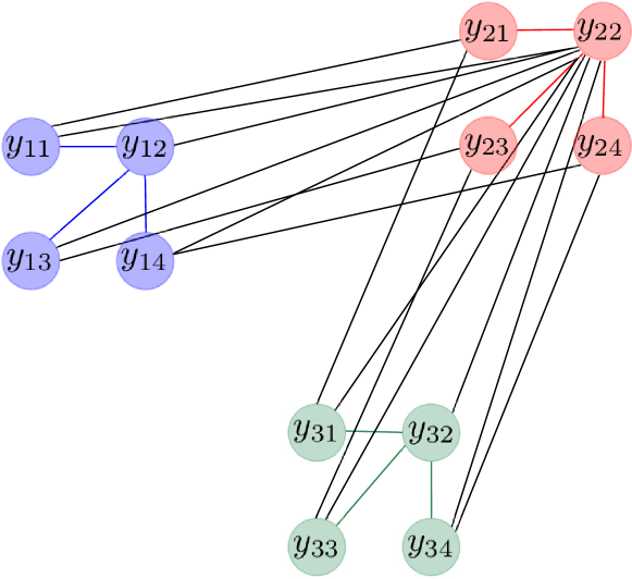
Figure 1: An example of dynamic KGM with $m_{1}=3$ modules (red, blue and green) composed by $m_{2}=4$ nodes. $y=[\,y_{11}\,y_{12}\,y_{13}\,y_{14}\,y_{21}\,y_{22}\,y_{23}\,y_{24}\,y_{31}\,y_{32}\,y_{33}\,y_{34}\,]^{T}$, $\mathcal{E}_{1}=\{(1,2),(2,3)\}$ and $\mathcal{E}_{2}=\{(1,2),(2,3),(2,4)\}$.

Dahlhaus2000 showed that conditional dependence relations are characterized by the support of $\Phi^{-1}$. Therefore, in our case an equivalent condition of (2) is

$$\mathrm{supp}(\Phi^{-1})=E_{1}\otimes E_{2}$$ (6)

where $E_{1}$ and $E_{2}$ are adjacency matrices of dimension $m_{1}\times m_{1}$ and $m_{2}\times m_{2}$, respectively, such that $(E_{1})_{hj}=1$ if and only if $(h,j)\in\mathcal{E}_{1}$ otherwise $(E_{1})_{hj}=0$ and likewise for $E_{2}$ and $\mathcal{E}_{2}$. In other words, $y$ corresponds to a dynamic KGM if and only if condition (6) holds. The next proposition shows that $\mathcal{E}_{1}$ and $\mathcal{E}_{2}$ describe the conditional dependence relations among modules and nodes in each module, respectively.

Proposition 1.

Consider the vector spaces

$$\chi^{\star}_{I_{1}} =\overline{\mathrm{span}}\{\,y_{hk}(t)\hbox{ s.t. }\,h\in I_{1},\,k\in\mathcal{V}_{2},\,t\in\mathbb{Z}\,\}$$ (7)

$$\chi^{\dagger}_{I_{2}} =\overline{\mathrm{span}}\{\,y_{hk}(t)\hbox{ s.t. }\,h\in\mathcal{V}_{1},\,k\in I_{2},\,t\in\mathbb{Z}\,\}$$ (8)

where $I_{1}\subseteq\mathcal{V}_{1}$ and $I_{2}\subseteq\mathcal{V}_{2}$. Under assumption (6) we have that

$$(h,j)\notin\mathcal{E}_{1}\;\iff\;\chi_{\{h\}}^{\star}\,\bot\,\chi_{\{j\}}^{\star}\,|\,\chi^{\star}_{\mathcal{V}_{1}\setminus\{h,j\}}$$ (9)

$$(k,l)\notin\mathcal{E}_{2}\;\iff\;\chi_{\{k\}}^{\dagger}\,\bot\,\chi_{\{l\}}^{\dagger}\,|\,\chi^{\dagger}_{\mathcal{V}_{2}\setminus\{k,l\}}.$$ (10)

Proof 2.1.

We prove condition (9); condition (10) can be proved in a similar way. Let

$$z_{h}(t)=[\,y_{h1}(t)\ldots y_{hm2}(t)\,]^{T}.$$ (11)

Let $\varepsilon(t)=[\,\varepsilon_{h}(t)^{T}\,\varepsilon_{j}(t)^{T}\,]^{T}$ be the projection error of $[\,z_{h}(t)^{T}\,z_{j}(t)^{T}\,]^{T}$ onto $\chi^{\star}_{\mathcal{V}_{1}\setminus\{h,j\}}$ with $h\neq j$. Since $\varepsilon$ is a zero mean Gaussian stationary process, proving (9) is equivalent to prove that

$$(h,j)\notin\mathcal{E}_{1}\,\iff\,\mathbb{E}[\varepsilon_{h}(t)\varepsilon_{j}(t)^{T}]=0,\;\;\forall\,t\in\mathbb{Z}.$$ (12)

Let $P_{\Pi}$ be the permutation matrix that permutes the components of $y$ in order to obtain

$$\tilde{y}=P_{\Pi}y=\left[\begin{array}[]{c}z_{h}\\ z_{j}\\ \hline\cr z_{k\neq h,i}\end{array}\right]=\left[\begin{array}[]{c}\tilde{y}_{1}\\ \hline\cr\tilde{y}_{2}\\ \end{array}\right]$$ (18)

where $z_{k\neq h,j}$ is the process obtained by stacking $z_{k}$ with $k\neq h,j$. We partition the PSD $\tilde{\Phi}$ of $\tilde{y}$ in conformable way

$$\tilde{\Phi}=\left[\begin{array}[]{cc}\tilde{\Phi}_{1,1}&\tilde{\Phi}_{1,2}\\ \tilde{\Phi}_{2,1}&\tilde{\Phi}_{2,2}\\ \end{array}\right].$$ (21)

Notice that

$$\tilde{\Phi}^{-1}=P_{\Pi}\Phi^{-1}P_{\Pi}^{T}=\left[\begin{array}[]{cc}\Sigma&\hskip 8.5359pt\star\\ \star&\hskip 8.5359pt\star\\ \end{array}\right]$$ (24)

where

$$\Sigma^{-1}=\tilde{\Phi}_{1,1}-\tilde{\Phi}_{1,2}\tilde{\Phi}_{2,2}^{-1}\tilde{\Phi}_{2,1}=\tilde{\Phi}_{\varepsilon}$$ (25)

and $\tilde{\Phi}_{\varepsilon}$ denotes the PSD of $\varepsilon$. Therefore, $\mathbb{E}[\varepsilon_{h}(t)\varepsilon_{j}(t)^{T}]=0$ $\forall\,t\in\mathbb{Z}$ if and only if $\Sigma$ is block-diagonal (according to the partition in $\varepsilon(t)=[\,\varepsilon_{h}(t)^{T}\,\varepsilon_{j}(t)^{T}\,]^{T}$). In view of (6), $\Sigma$ is block-diagonal if and only if $(h,j)\notin\mathcal{E}_{1}$. We conclude that (12) holds. ∎

Throughout the paper we want to address the following identification problem about dynamic KGM.

Problem 2.

Consider an AR Gaussian zero mean full rank stationary stochastic process $y$ of order $n$ and taking values in $\mathbb{R}^{m_{1}m_{2}}$. Assume that $m_{1}$, $m_{2}$, $n$ are known and collect a finite length sequence $y^{N}:=\{y(1),y(2)\ldots y(N)\}$ extracted from a realization of $y$. Let $\Phi$ be the PSD of $y$ satisfying (6). Find an estimate $\hat{\Phi}$ of $\Phi$ from $y^{N}$ such that $\mathrm{supp}(\hat{\Phi}^{-1})=\hat{E}_{1}\otimes\hat{E}_{2}$ where $\hat{E}_{1}$ and $\hat{E}_{2}$ represent an estimate of $E_{1}$ and $E_{2}$, respectively.

It is worth noting that condition (6) is weaker than $\Phi^{-1}$ admit a Kronecker decomposition, i.e. $\Phi^{-1}=\Phi^{-1}_{1}\otimes\Phi^{-1}_{2}$. Accordingly, we do not constrain the dynamics in each module to be same. In what follows we present some practical problems in which a stochastic process corresponding to a dynamic KGM could be used.

2.1 Dynamic spatio-temporal modeling

Consider a non-stationary zero mean Gaussian process $x=\{x(\tilde{t}),\;\tilde{t}\in\mathbb{Z}\}$ indexed by the time variable $\tilde{t}$ where $x(\tilde{t})$ takes values in $\mathbb{R}^{m_{2}}$, $m_{2}\in\mathbb{N}$, and whose covariance lags sequence $P_{\tilde{t},\tilde{s}}=\mathbb{E}[x(\tilde{t})x(\tilde{t}+\tilde{s})^{T}]$ is such that

$$P_{\tilde{t}+m_{1},\tilde{s}}=P_{\tilde{t},\tilde{s}},\;\;\;\tilde{t},\tilde{s}\in\mathbb{Z}$$ (26)

with $m_{1}\in\mathbb{N}$. We can rewrite $x$ in terms of the stochastic process $y=\{y(t),\;t\in\mathbb{Z}\}$ defined as

$$y(t)=[\,x((t-1)m_{1}+1)^{T}\ldots x(tm_{1})^{T}\,]^{T}.$$ (27)

It is worth noting that the time variables $\tilde{t}$ and $t$ are different: there is a decimation relationship between them and the decimation factor is $m_{1}$. It is not difficult to see that $y$ is zero mean, Gaussian and stationary. In particular, its covariance lags sequence $R_{s}=\mathbb{E}[y(t)y(t+s)^{T}]$ is

$$R_{s}=\left[\begin{array}[]{cccccc}P_{1,sm_{1}}&P_{1,sm_{1}+1}&\ldots&\ldots&\ldots&P_{1,(s+1)m_{1}-1}\\ P_{1,sm_{1}+1}^{T}&P_{2,sm_{1}}^{T}&\ddots&&&\vdots\\ \vdots&\ddots&\ddots&&&\vdots\\ \vdots&&&&&P_{m_{1}-1,sm_{1}+1}\\ P_{1,(s+1)m_{1}-1}^{T}&\ldots&\ldots&\ldots&P_{m_{1}-1,sm_{1}+1}^{T}&P_{m_{1},sm_{1}}\end{array}\right]$$ (33)

where we have exploited the relation $P_{\tilde{t},\tilde{s}}^{T}=P_{\tilde{t}+\tilde{s},-\tilde{s}}$. Let $\Phi$ be the PSD of $y$ and assume that condition (6) holds. In view of Proposition 1, with $y_{hk}(t)=x_{k}((t-1)m_{1}+h)$, $\mathcal{E}_{2}$ describes the conditional dependence relations among the components $x_{k}$, with $k\in\mathcal{V}_{2}$, of process $x$. We conclude that $x$ can be understood as a spatio-temporal process. In the special case that

$$P_{\tilde{t},\tilde{s}}=0,\;\;\forall\,\tilde{s}\hbox{ s.t. }|\tilde{s}|\geq m_{1}$$ (34)

we have that $R_{s}=0$ for any $s>0$ and thus $y$ is an i.i.d. Gaussian process, i.e. $\Phi$ is a covariance matrix. The latter models magnetoencephalography (MEG) measurements used for mapping brain activity, bijma2005spatiotemporal. More precisely, $z_{k}(t)=[\,x_{k}((t-1)m_{1}+1)\,\ldots\,x_{k}(tm_{1})\,]^{T}$ models the measurements at the $k$-th brain area during the $t$-th trial of length $m_{1}$. All the trials are independent. Moreover, the latter are identically distributed because in each trial the patient is required to perform the same cognitive task. In our framework we can remove condition (34), i.e. the trials now can be dependent. This means that in the future such trials can be scheduled in a sequential way and modeled through the spatio-temporal process $x$. In view of Proposition 1, $\mathcal{E}_{2}$ describes the conditional dependence relations between the different brain areas. It is worth noting that we do not force the Kronecker structure on $\Phi^{-1}$: such freedom has shown to be crucial for an effective MEG modeling. Finally, the spatio-temporal process $x$ can be potentially used also to urban pollution monitoring, see Section LABEL:sec:sec:poll.

2.2 Multi-task modeling

We consider a network composed by $m_{2}\in\mathbb{N}$ agents (i.e. nodes); each agent is described by a zero mean Gaussian stationary stochastic process. We want to model such a network under $m_{1}\in\mathbb{N}$ heterogeneous conditions (i.e. tasks). Let $y_{hk}=\{y_{hk}(t),\;t\in\mathbb{Z}\}$ denote the stochastic process describing the $k$-th agent under the $h$-th task. Then, we can model the network through the $m_{1}$ stochastic processes

$$w_{h}=[\,y_{h1}\,\ldots\,y_{hm_{2}}\,]^{T},\;\;\;h\in\mathcal{V}_{1}$$ (35)

where $h$ denotes the task. A more flexible approach is to model all processes in (35) together in order to exploit commonalities and differences across the tasks, see allen2010transposable; yu2009large. More precisely, we consider the stationary stochastic process $y$ obtained by stacking $w_{h}$ with $h\in\mathcal{V}_{1}$. Let $\Phi$ be the PSD of $y$ and such that (6) holds. In view of Proposition 1, $\mathcal{E}_{1}$ describes the conditional dependence relations among the tasks, while $\mathcal{E}_{2}$ describes the ones among the agents of the network. It is worth noting that our model is dynamic in contrast with the ones in allen2010transposable; yu2009large which are static. The proposed model could be used to describe the travel demand in a public transport system of a certain city network, chidlovskii2017multi. More precisely, $y_{hk}(t)$ denotes the total number of boarding events at day $t$, $k$ represents a particular area in the city network and $h$ represents the type of transportation (e.g. bus, train, tram).

3 Identification of KGM

We aim to solve Problem 2 where we parametrize the PSD of $y$ as $\Phi=\Sigma^{-1}$ where $\Sigma\in\mathcal{Q}_{m,n}$, $m=m_{1}m_{2}$ and

$$\Sigma(e^{i\theta})=S_{0}+\frac{1}{2}\sum_{t=1}^{n}[S_{t}e^{-it\vartheta}+S_{t}^{T}e^{it\vartheta}].$$ (36)

Notice that

$$(\Sigma(e^{i\vartheta}))_{hk,jl}$$

$$=(S_{0})_{hk,jl}+\frac{1}{2}\sum_{t=1}^{n}[(S_{t})_{hk,jl}e^{-it\vartheta}+(S_{t})_{jl,hk}e^{it\vartheta}]$$

where $(\Sigma)_{hk,jl}$ denotes the entry of $\Sigma$ with row $(h-1)m_{2}+k$ and column $(j-1)m_{2}+l$ with $h,j\in\mathcal{V}_{1}$ and $k,l\in\mathcal{V}_{2}$; the same meaning has the notation $(S_{t})_{hk,jl}$ for $S_{t}$. We consider the following regularized ML estimator of $\Sigma$, and thus of $\Phi$:

$$\hat{\Sigma}= \underset{\Sigma\in\mathcal{Q}_{m,n}}{\mathrm{argmin}}\,\ell(y^{N};\Sigma)+g(\Sigma;\Lambda,\Gamma)$$

$$\hbox{ s.t. }\Sigma\in\mathcal{Q}_{m,n}^{+}$$ (37)

where $\mathcal{Q}_{m,n}^{+}:=\{\Sigma\in\mathcal{Q}_{m,n}\hbox{ s.t. }\Sigma\succ 0\}$. The term $\ell(y^{N};\Sigma)$ is an approximation of the negative log-likelihood of $y(n+1)\ldots y(N)$ given $y(1)\ldots y(n)$ under the assumption that $y$ is an AR process of order $n$:

$$\ell(y^{N};\Sigma)=\frac{N-n}{4\pi}\int_{-\pi}^{\pi}[-\log|\Sigma|+\mathop{\rm tr}(\hat{\Phi}_{p}\Sigma)]\mathrm{d}\vartheta+c$$ (38)

where

$$\color[rgb]{0,0,0}\hat{\Phi}_{p} =\color[rgb]{0,0,0}\hat{R}_{0}+\frac{1}{2}\sum_{s=1}^{n}[\hat{R}_{s}e^{-is\vartheta}+\hat{R}_{s}^{T}e^{is\vartheta}]$$

$$\hat{R}_{s} =\frac{1}{N-n}\sum_{t=1}^{N-s}y(t)y(t+s)^{T}$$ (39)

and $c$ is a term not depending on $y^{N}$ and $\Sigma$. Notice that $\hat{R}_{s}$ represents an estimate of $R_{s}$ from data $y^{N}$ and $\hat{\Phi}_{p}$ is the truncated periodogram of $\Phi$. Let $\mathrm{T}(\hat{R})$ denote the block-Toeplitz matrix whose first block row is $[\,\hat{R}_{0}\,\hat{R}_{1}\ldots\hat{R}_{n}\,]$. Throughout the paper we make the assumption that $\mathrm{T}(\hat{R})\succ 0$. The latter assumption holds for $N$ sufficiently large since $y$ is a full rank process. The penalty term $g(\Sigma;\Lambda,\Gamma)$ induces some desired properties in the solution $\hat{\Sigma}$; $\Lambda$ and $\Gamma$ are the regularization matrices (hereafter called hyperparameter matrices) that later will be estimated from the data. REWEIGHTED proposed the following penalty term, which in turn is built on the one by SONGSIRI_TOP_SEL_2010, for estimating a SGM:

$$g(\Sigma; \Omega)=\sum_{(h,k,j,l)\in\mathcal{T}_{S}}(\Omega)_{hk,jl}\times$$

$$\times\max\{\max_{t=0\ldots n}|(S_{t})_{hk,jl}|,\max_{t=0\ldots n}|(S_{t})_{jl,hk}|\}$$ (40)

where $\mathcal{T}_{S}=\{(h,k,j,l)\hbox{ s .t. }(h-1)m_{2}+k\geq(j-1)m_{2}+l\}$ and the entries of the weight symmetric matrix $\Omega$ are estimated using an approximate version of the empirical Bayes approach. It has been shown that (3) leads to an estimate of $\Phi$ whose inverse is sparse. Here, instead, we consider a penalty term $g(\,\cdot\,;\Lambda,\Gamma)\,:\,\mathcal{Q}_{m,n}\longrightarrow\mathbb{R}$ which is designed in such a way to induce (6) in the solution of (3). More precisely, we consider

$$g (\Sigma;\Lambda,\Gamma)=\sum_{(h,k,j,l)\in\mathcal{T}}\max\{\lambda_{hj},\gamma_{kl}\}q_{hk,jl}(\Sigma)$$ (41)

with

$$\mathcal{T}:=\{(h,k,j,l)\hbox{ s.t. }h,j\in\mathcal{V}_{1}\;k,l\in\mathcal{V}_{2}\hbox{ and }h\geq j,\;k\geq l\}$$

$$q_{hk,jl}(\Sigma):=\max\{\max_{t=0\ldots n}|(S_{t})_{hk,jl}|,\max_{t=0\ldots n}|(S_{t})_{hl,jk}|,$$

$$\hskip 76.82234pt\max_{t=0\ldots n}|(S_{t})_{jl,hk}|,\max_{t=0\ldots n}|(S_{t})_{jk,hl}|\},$$

$\lambda_{hj},\gamma_{kl}\geq 0$, with $h,j\in\mathcal{V}_{1}$ and $k,l\in\mathcal{V}_{2}$.

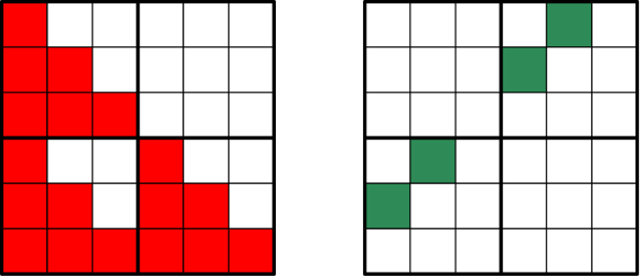
Figure 2: Example with $m_{1}=2$ and $m_{2}=3$. Left. In red the positions of $S_{t}$ which are taken in $\mathcal{T}$. Right. In green the entries of $S_{t}$ which are considered in $q_{hk,jl}(\Sigma)$ with $h=2$, $j=1$, $k=2$, $l=1$.

It is worth noting that the index set $\mathcal{T}$ contains only a subset of all the possible indexes characterizing the entries of $\Sigma$, see Figure 2 (left). This is because the support of $\Sigma$ has to satisfy the symmetric Kronecker structure in (6), indeed recall that $E_{1}$ and $E_{2}$ are symmetric adjacency matrices. Accordingly, we induce a group sparsity not only to guarantee that $St$’s have the same support but also to guarantee the symmetric property in (6), see the example of Figure 2 (right). $\lambda_{hj}$ and $\gamma_{kl}$ are the entries in position $(h,j)$ and $(k,l)$ of the symmetric matrices $\Lambda$ and $\Gamma$, respectively. Notice that $\Lambda$ and $\Gamma$ are nonnegative matrices of dimension $m_{1}\times m_{1}$ and $m_{2}\times m_{2}$, respectively. Some comments about this penalty term follow. $g(\Sigma;\Lambda,\Gamma)$ is a weighted sum of the nonnegative terms $q_{hk,jl}(\Sigma)$, so the penalty induces many of these terms to be equal to zero. If $q_{hk,jl}(\Sigma)=0$, then $(\Sigma)_{hk,jl}$, $(\Sigma)_{jl,hk}$, $(\Sigma)_{hl,jk}$ and $(\Sigma)_{jk,hl}$ coincide with the null function. Therefore, such a penalty encourages a common sparsity pattern (i.e. group sparsity, see as example DUE) on $\Sigma$ according to (6). More precisely, if $\lambda_{hj}$ is large then it is more likely that the solution of (3) is such that $q_{hk,jl}(\Sigma)=0$ for any $k,l\in\mathcal{V}_{2}$, i.e. (6) holds with $(h,j)\notin\mathcal{E}_{1}$. If $\gamma_{kl}$ is large then it is more likely that the solution of (3) is such that $q_{hk,jl}(\Sigma)=0$ for any $h,j\in\mathcal{V}_{1}$, i.e. (6) holds with $(k,l)\notin\mathcal{E}_{2}$.

Proposition 3.

The objective function of Problem (3) is strictly convex in $\Sigma$. Moreover, Problem (3) admits a unique solution.