An energetically balanced, quasi-Newton integrator for non-hydrostatic vertical atmospheric dynamics

Abstract

An energetically balanced, implicit integrator for non-hydrostatic vertical atmospheric dynamics on the sphere is presented. The integrator allows for the exact balance of energy exchanges in space and time for vertical atmospheric motions by preserving the skew-symmetry of the non-canonical Hamiltonian formulation of the compressible Euler equations. The performance of the integrator is accelerated by a preconditioning strategy that reduces the dimensionality of the inner linear system. Here we reduce the four component velocity, density, density weighted potential temperature and Exner pressure system into a single equation for the density weighted potential temperature via repeated Schur complement decomposition and the careful selection of coupling terms. As currently formulated, the integrator is based on a horizontal-vertical spatial splitting that does not permit bottom topography. The integrator is validated for standard test cases for baroclinic instability and a non-hydrostatic gravity wave on the sphere and a rising bubble in a high-resolution planar geometry, and shows robust convergence across all of these regimes.

1 Introduction

Energy conserving, semi-implicit time integrators for various geophysical systems in Hamiltonian form have been previously introduced for the shallow water [1, 2] and thermal shallow water [3, 4] equations on the sphere, and the compressible Euler equations in vertical slice geometry [4]. They have also been implemented on other areas, such as plasma physics [5]. These integrators are based on discrete gradient methods [6, 7] for non-canonical Hamiltonian systems which preserve the skew-symmetric property of the Poisson bracket in the spatial discretisation and the exact integration of the variational derivatives of the Hamiltonian in the temporal discretisation. In doing so these integrators satisfy the exact balance of energy exchanges, as well as the orthogonality of the vorticity dynamics to these energetic exchanges. By mitigating against internal biases in the representation of dynamical processes these integrators may help to improve the statistical quality of long time integrations.

In the present article a skew-symmetric mimetic spectral element spatial discretisation of the 3D compressible Euler equations on the sphere [8] is extended to incorporate such an integrator for non-hydrostatic vertical dynamics. The vertical integrator is coupled to the explicit horizontal dynamics using a trapazoidal horizontally explicit/vertically implicit (HEVI) splitting scheme [9, 10], which complements the centered time integration of the vertical scheme. Skew-symmetric formulations have previously been used as the basis for energy conserving spatial discretisations of vertical dynamics in non-hydrostatic atmospheric modelling [11]. In order to accelerate the performance of such an integrator, Schur complement reduction may be applied in order to transform the coupled nonlinear system into a single equation at each linear solve [12, 13]. In the present formulation the coupled velocity, density, density weighted potential temperature, Exner pressure system is reduced to a single equation for the density weighted potential temperature, for which the implicit Helmholtz operator incorporates corrections to both the gradient and divergence operators in order to account for the thermodynamics. This operator is derived from the reduction of an approximate Jacobian for a deliberate choice of coupling terms.

The motivation for such an integrator is twofold. Firstly, almost all of the energy of the atmosphere exists as either potential or internal energy, which are dependent on the density and potential temperature (or equivalent thermodynamic variables). These quantities are strongly stratified, such that their gradients are much sharper in the vertical dimension than the horizontal. As such it is hoped that by balancing energetic exchanges associated with transient vertical processes this will improve the overall representation of dynamics within the model. Secondly, by developing such an integrator and demonstrating its robust performance across different scales and physical regimes, this may inform the development of a fully three-dimensional energetically balanced integrator.

In section 2 the 3D compressible Euler equations are introduced in continuous form, including a brief discussion of their energetic properties. Section 3 briefly describes the mixed mimetic spectral element spatial discretisation of the 3D compressible Euler equations [8]. For more extensive discussions of this discretisation [14, 15] and its properties for geophysical flow simulation [16, 17] the reader is referred to the aforementioned articles. The energetic properties of the spatially and temporally discrete system are discussed in section 4. Section 5 describes the formulation of the quasi-Newton vertical integrator, including the nonlinear preconditioning strategy. Results for the reproduction of standard test cases are presented in section 6, and finally conclusions and discussion of future work are presented in section 7.

2 The rotating 3D compressible Euler equations

The three dimensional compressible Euler equations for a shallow atmosphere may be expressed as [18, 19, 8]

$$\frac{\partial\bm{u}}{\partial t}+(\bm{\omega}+\bm{f})\times\bm{u}+\nabla\Bigg{(}\frac{1}{2}\|u\|^{2}+gz\Bigg{)}+\theta\nabla\Pi =0,$$ (1a)

$$\frac{\partial\rho}{\partial t}+\nabla\cdot(\rho\bm{u}) =0,$$ (1b)

$$\frac{\partial\rho\theta}{\partial t}+\nabla\cdot(\rho\theta\bm{u}) =0,$$ (1c)

where $\bm{u}=u\bm{e}_{\lambda}+v\bm{e}_{\varphi}+w\bm{e}_{z}$ are the zonal, meridional and vertical velocity components respectively, $\rho$ is the density, $\bm{f}=f\bm{e}_{z}$ is the Coriolis term, $g$ is the acceleration due to gravity, $\theta$ is the potential temperature, and $\Pi$ is the Exner pressure (including the specific heat at constant pressure). The potential temperature and Exner pressure are defined with respect to the standard thermodynamic variables of temperature, $T$, and pressure, $p$, as

$$\Pi :=c_{p}\Bigg{(}\frac{p}{p_{0}}\Bigg{)}^{\frac{R}{c_{p}}},$$ (2a)

$$\theta :=\frac{c_{p}T}{\Pi},$$ (2b)

where $c_{p}$ is the specific heat at constant pressure, $p_{0}$ is the reference pressure, and $R=c_{p}-c_{v}$ is the ideal gas constant (and $c_{v}$ is the specific heat at constant volume). Using (2) the ideal gas law, $p=R\rho T$ may be reformulated as

$$\Pi=c_{p}\Bigg{(}\frac{R\rho\theta}{p_{0}}\Bigg{)}^{\frac{R}{c_{v}}}.$$ (3)

To obtain a closed system for the solution of the compressible Euler equations, (1) and (3) must be supplemented by appropriate boundary conditions. We impose homogeneous Dirichlet boundary conditions on the $z$-component of velocity, $w$ as

$$\left.w\right|_{z=0}=\left.w\right|_{z=z^{\mathrm{top}}}=0,$$ (4)

where $z^{\mathrm{top}}$ corresponds to the $z$-coordinates of the top boundary of the domain. We also apply homogeneous Neumann boundary conditions on the Exner pressure as

$$\frac{\partial\Pi}{\partial z}\Bigg{|}_{z=0}=\frac{\partial\Pi}{\partial z}\Bigg{|}_{z=z^{top}}=0.$$ (5)

Note that in this formulation we have invoked the shallow atmosphere approximation, for which gravity is constant throughout the fluid column and the height of the fluid column is negligible with respect to the earth’s radius. We further assume that the horizontal components of the Coriolis term are small and omit these from the formulation [20].

2.1 Energetics

In this section the energetics of the 3D compressible Euler equations will be briefly analysed in continuous form. The energetics of the discrete formulation will be discussed in subsequent sections.

2.1.1 Kinetic, potential, and internal energy

The kinetic energy, $K$, is defined as

$$K:=\frac{1}{2}\langle\bm{u},\rho\bm{u}\rangle=\frac{1}{2}\int_{\Omega}\rho\|u\|^{2},$$ (6)

where $\|u\|:=\langle\bm{u},\bm{u}\rangle$, and $\langle\cdot,\cdot\rangle$ is the $L^{2}$ inner product given for scalar fields as

$$\langle f,g\rangle:=\int_{\Omega}fg\,\mathrm{d}\Omega\,,$$ (7)

and for vector fields as

$$\langle\bm{u},\bm{v}\rangle:=\int_{\Omega}\bm{u}\cdot\bm{v}\,\mathrm{d}\Omega.$$ (8)

The time variation of kinetic energy is obtained by summing the $L^{2}$ inner product, between the momentum equation, (1a), and $\rho\bm{u}$, and between the continuity equation, (1b), and $\frac{1}{2}\|u\|^{2}$

$$\frac{\partial K}{\partial t}=-\langle g,\rho w\rangle-\langle\rho\bm{u},\theta\nabla\Pi\rangle\,,$$ (9)

where again $w$ is the $z$-component of the velocity field, $\bm{u}$.

The potential energy, $P$, is given by

$$P:=\left\langle\rho\,,\,gz\right\rangle=\int_{\Omega}\rho gz\,\mathrm{d}\Omega,$$ (10)

and its time derivative follows directly

$$\frac{\partial P}{\partial t}=\left\langle gz\,,\,\frac{\partial\rho}{\partial t}\right\rangle\stackrel{{\scriptstyle\eqref{eq::dens}}}{{=}}-\langle gz,\nabla\cdot(\rho\bm{u})\rangle=\langle g,\rho w\rangle\,,$$ (11)

where we have used integration by parts on the last identity and assumed periodic boundary conditions in the horizontal directions, together with homogeneous boundary conditions for the vertical component of the velocity field, (4).

The internal energy, $I$, is defined as

$$I:=\int_{\Omega}c_{v}\rho T\,\mathrm{d}\Omega\stackrel{{\scriptstyle\eqref{eq:potential_temperature_definition}}}{{=}}\int_{\Omega}\frac{c_{v}}{c_{p}}\rho\theta\Pi\,\mathrm{d}\Omega=\int_{\Omega}c_{v}\rho\theta\left(\frac{R\rho\theta}{p_{0}}\right)^{\frac{R}{c_{v}}}\,\mathrm{d}\Omega=\int_{\Omega}c_{v}\left(\frac{R}{p_{0}}\right)^{\frac{R}{c_{v}}}\left(\rho\theta\right)^{\frac{c_{p}}{c_{v}}}\,\mathrm{d}\Omega\,.$$ (12)

After some manipulation, the time variation of internal energy is given by

$$\frac{\partial I}{\partial t}=-\left\langle\nabla\cdot(\rho\theta\bm{u})\,,\,\Pi\right\rangle=\left\langle\rho\bm{u}\,,\,\theta\nabla\Pi\right\rangle\,.$$ (13)

where integration by parts was used on the last identity, together with homogeneous boundary conditions for $\bm{u}$ and periodic boundary conditions on the horizontal directions. Note that the substitution of the boundary conditions as defined in (4) and (5) into (9), (11) and (13) ensures that there is no temporal change in energy at the boundary. Mass conservation is also ensured by the substitution of (4) into (1b).

2.1.2 Conservation of total energy

Following [19], the total energy, $\mathcal{H}$, is given as the sum of kinetic, $K$, potential, $P$, and internal, $I$, energy as

$$\mathcal{H}:=K+P+I=\int_{\Omega}\frac{1}{2}\rho u^{2}\,\mathrm{d}\Omega+\int_{\Omega}\rho gz\,\mathrm{d}\Omega+\int_{\Omega}\frac{c_{v}}{c_{p}}\Theta\Pi\,\mathrm{d}\Omega\,.$$ (14)

where $\Theta:=\rho\theta$. The variational derivatives of $\mathcal{H}$ with respect to the prognostic variables $\bm{u}$, $\rho$, and $\Theta$, are given as

$$\frac{\delta\mathcal{H}}{\delta\bm{u}}=\rho\bm{u}=\bm{U},\qquad\frac{\delta\mathcal{H}}{\delta\rho}=\frac{1}{2}u^{2}+gz=\Phi,\qquad\frac{\delta\mathcal{H}}{\delta\Theta}=\Pi.$$ (15)

Writing the prognostic variables as a column vector of the form, $\bm{\mathsf{a}}=[\bm{u}\quad\rho\quad\Theta]^{\top}$, we may then express the original system (1) as [21]

$$\frac{\partial\bm{\mathsf{a}}}{\partial t}=\bm{\mathsf{B}}\,\frac{\delta\mathcal{H}}{\delta\bm{\mathsf{a}}},$$ (16)

where $\bm{\mathsf{B}}$ is a skew-symmetric operator of the form

$$\bm{\mathsf{B}}:=\left[\begin{array}[]{ccc}-\bm{q}\times(\cdot)&-\nabla(\cdot)&-\theta\nabla(\cdot)\\ -\nabla\cdot(\cdot)&0&0\\ -\nabla\cdot(\theta\cdot)&0&0\\ \end{array}\right],$$ (17)

and $\bm{q}=(\bm{\omega}+\bm{f})/\rho$ is the potential vorticity. Energy conservation is then assured since

$$\frac{\partial\mathcal{H}}{\partial t}=\frac{\delta\mathcal{H}}{\delta\bm{\mathsf{a}}}\cdot\frac{\partial\bm{\mathsf{a}}}{\partial t}\stackrel{{\scriptstyle\eqref{eq:da_dt_B_H}}}{{=}}\frac{\delta\mathcal{H}}{\delta\bm{\mathsf{a}}}\cdot\left(\bm{\mathsf{B}}\frac{\delta\mathcal{H}}{\delta\bm{\mathsf{a}}}\right)=0,$$ (18)

where the last identity follows from the skew-symmetry of $\bm{\mathsf{B}}$.

3 Spatial discretisation

In this section we briefly describe some of the important features of the mixed mimetic spectral element spatial discretisation used in this work. For a complete description of this discretisation as it applies to the 3D compressible Euler equations on the cubed sphere see [8].

The mixed mimetic spectral element method [14, 15] is a compatible family of finite element spaces. For finite dimensional polynomial spaces of the form $\mathcal{P}_{h}(\Omega)\subset H^{1}(\Omega)$, $\mathcal{W}_{h}(\Omega)\subset H(\mathrm{curl},\Omega)$, $\mathcal{U}_{h}(\Omega)\subset H(\mathrm{div},\Omega)$, and $\mathcal{Q}_{h}(\Omega)\subset L^{2}(\Omega)$ the discrete analogues of the differential operators satisfy a series of compatibility relations of the form

$$\mathbb{R}\longrightarrow\mathcal{P}_{h}(\Omega)\stackrel{{\scriptstyle\nabla}}{{\longrightarrow}}\mathcal{W}_{h}(\Omega)\stackrel{{\scriptstyle\nabla\times}}{{\longrightarrow}}\mathcal{U}_{h}(\Omega)\stackrel{{\scriptstyle\nabla\cdot}}{{\longrightarrow}}\mathcal{Q}_{h}(\Omega)\longrightarrow 0,$$ (19)

where the space $H^{1}(\Omega)$ represents square integrable functions over $\Omega$ whose gradient is also square integrable, $H(\mathrm{curl},\Omega)$ and $H(\mathrm{div},\Omega)$ contain square integrable vector fields over $\Omega$ with square integrable curl and divergence respectively, and the function space $L^{2}(\Omega)$ contains square integrable functions. Each of these polynomial function spaces has an associated finite set of basis functions $\epsilon^{\mathcal{P}}_{i}$, $\bm{\epsilon}^{\mathcal{W}}_{i}$, $\bm{\epsilon}^{\mathcal{U}}_{i}$, and $\epsilon^{\mathcal{Q}}_{i}$, such that

$$\mathcal{P}_{h}=\mathrm{span}\{\epsilon^{\mathcal{P}}_{1},\dots,\epsilon^{\mathcal{P}}_{d_{\mathcal{P}}}\},\quad\mathcal{W}_{h}=\mathrm{span}\{\bm{\epsilon}^{\mathcal{W}}_{1},\dots,\bm{\epsilon}^{\mathcal{W}}_{d_{\mathcal{W}}}\},\quad\mathcal{U}_{h}=\mathrm{span}\{\bm{\epsilon}^{\mathcal{U}}_{1},\dots,\bm{\epsilon}^{\mathcal{U}}_{d_{\mathcal{U}}}\},\quad\mathrm{and}\quad\mathcal{Q}_{h}=\mathrm{span}\{\epsilon^{\mathcal{Q}}_{1},\dots,\epsilon^{\mathcal{Q}}_{d_{\mathcal{Q}}}\}.$$ (20)

The discrete mappings given in (19) are represented by strong form topological relations as [14]:

$$\nabla\epsilon^{\mathcal{P}}_{j}=\sum_{k=0}^{d_{\mathcal{W}}}\mathsf{E}_{k,j}^{1,0}\bm{\epsilon}^{\mathcal{W}}_{k},\qquad\nabla\times\bm{\epsilon}^{\mathcal{W}}_{j}=\sum_{k=0}^{d_{\mathcal{U}}}\mathsf{E}_{k,j}^{2,1}\bm{\epsilon}^{\mathcal{U}}_{k},\qquad\mathrm{and}\qquad\nabla\cdot\bm{\epsilon}^{\mathcal{U}}_{j}=\sum_{k=0}^{d_{\mathcal{Q}}}\mathsf{E}_{k,j}^{3,2}\epsilon^{\mathcal{Q}}_{k},$$ (21)

where $\bm{\mathsf{E}}^{1,0}$, $\bm{\mathsf{E}}^{2,1}$, and $\bm{\mathsf{E}}^{3,2}$ are so called incidence matrices corresponding to the discrete versions of the differential operators grad, curl and div. Conversely, reverse mappings may be applied through weak form adjoints to these operators [15].

3.1 Directional splitting

Here we briefly describe the splitting procedure used to decompose the three dimensional problem into horizontal (two dimensional) and vertical sub-problems. Due to the nature of the various function spaces, this splitting implies no additional approximation to the spatial discretisation. However this construction does involve a temporal approximation, by which the horizontal and vertical sub problems are solved explicitly and implicitly respectively [9, 10].

We defined the horizontal, $\bm{u}_{\parallel}$, and vertical, $\bm{u}_{\perp}$, components of the velocity field $\bm{u}=u\bm{e}_{\lambda}+v\bm{e}_{\varphi}+w\bm{e}_{z}$ as

$$\bm{u}_{\parallel}:=u\bm{e}_{\lambda}+v\bm{e}_{\varphi}\,,\qquad\bm{u}_{\perp}:=w\bm{e}_{z}\,.$$ (22)

Moreover, let $\nabla_{\parallel}$ and $\nabla_{\perp}$ represent the horizontal and vertical components of the gradient operator of a scalar field $\rho$

$$\nabla_{\parallel}\rho:=\frac{1}{a\cos(\phi)}\frac{\partial\rho}{\partial\lambda}\bm{e}_{\lambda}+\frac{1}{a}\frac{\partial\rho}{\partial\phi}\bm{e}_{\varphi}\,,\qquad\nabla_{\perp}\rho:=\frac{\partial\rho}{\partial z}\bm{e}_{z}\,.$$ (23)

In a similar way, $\nabla_{\parallel}\times$ and $\nabla_{\perp}\times$ represent, respectively, the horizontal and vertical components of the curl of a vector field $\bm{u}=u\bm{e}_{\lambda}+v\bm{e}_{\varphi}+w\bm{e}_{z}$

$$\nabla_{\parallel}\times\bm{u}:=\left(\frac{1}{a}\frac{\partial w}{\partial\phi}-\frac{\partial v}{\partial z}\right)\bm{e}_{\lambda}+\left(\frac{\partial u}{\partial z}-\frac{1}{a\cos(\phi)}\frac{\partial w}{\partial\lambda}\right)\bm{e}_{\varphi}\,,\qquad\nabla_{\perp}\times\bm{u}:=\frac{1}{a\cos(\phi)}\left(\frac{\partial v}{\partial\lambda}-\frac{\partial(\cos(\phi)u)}{\partial\phi}\right)\bm{e}_{z}\,.$$ (24)

Note that we have assumed the shallow atmosphere approximation of constant radius, $a$, in the above expressions. In practice, these spherical transformations are absorbed into the definition of the Jacobian [22] (including the shallow atmosphere approximation) and the associated Piola transformations for the different function spaces [17, 8].

From (23) and (24) it follows directly that

$$\nabla\rho=\nabla_{\parallel}\rho+\nabla_{\perp}\rho\,,\quad\mathrm{and}\quad\nabla\times\bm{u}=\nabla_{\parallel}\times\bm{u}+\nabla_{\perp}\times\bm{u}\,.$$

We may then reformulate the vorticity, $\bm{\omega}:=\nabla\times\bm{u}$, as

$$\bm{\omega}=\underbrace{\overbrace{\nabla_{\parallel}\times\bm{u}_{\parallel}}^{\bm{\omega}_{\parallel,\parallel}}+\overbrace{\nabla_{\parallel}\times\bm{u}_{\perp}}^{\bm{\omega}_{\parallel,\perp}}}_{\bm{\omega}_{\parallel}}+\underbrace{\nabla_{\perp}\times\bm{u}_{\parallel}}_{\bm{\omega}_{\perp}}\,.$$ (25)

While the spatial discretisation outlined above is valid for basis functions of any polynomial degree, $p$, in practice we use polynomials of arbitrary order in the horizontal only, and use a lowest order discretisation in the vertical for which the $\mathcal{P}_{h}$ bases are piecewise linear and the $\mathcal{Q}_{h}$ bases are piecewise constant [8].

Using (22), (23), (24), and (25), we may split the compressible Euler equations, (1), into horizontal and vertical components

$$\frac{\partial\bm{u}_{\parallel}}{\partial t}+(\bm{\omega}_{\perp}+\bm{f}_{\perp})\times\bm{u}_{\parallel}+\bm{\omega}_{\parallel,\parallel}\times\bm{u}_{\perp}+\frac{1}{2}\nabla_{\parallel}\|\bm{u}_{\parallel}\|^{2}+\theta\nabla_{\parallel}\Pi =0,$$ (26a)

$$\frac{\partial\bm{u}_{\perp}}{\partial t}+\bm{\omega}_{\parallel,\perp}\times\bm{u}_{\parallel}+\nabla_{\perp}\left(\frac{1}{2}\|\bm{u}_{\perp}\|^{2}+gz\right)+\theta\nabla_{\perp}\Pi =0,$$ (26b)

$$\frac{\partial\rho}{\partial t}+\nabla\cdot\left(\rho\bm{u}_{\parallel}\right)+\nabla\cdot\left(\rho\bm{u}_{\perp}\right) =0,$$ (26c)

$$\frac{\partial(\rho\theta)}{\partial t}+\nabla\cdot\left(\rho\theta\bm{u}_{\parallel}\right)+\nabla\cdot\left(\rho\theta\bm{u}_{\perp}\right) =0,$$ (26d)

where, as in (25), $\bm{\omega}_{\parallel,\parallel}:=\nabla_{\parallel}\times\bm{u}_{\parallel}$ and $\bm{\omega}_{\parallel,\perp}:=\nabla_{\parallel}\times\bm{u}_{\perp}$. The same splitting into horizontal and vertical components may be applied for the basis functions, (20),

$$\bm{\epsilon}^{\mathcal{W}}_{j}=\left(\bm{\epsilon}^{\mathcal{W}}_{j}\right)_{\parallel}+\left(\bm{\epsilon}^{\mathcal{W}}_{j}\right)_{\perp}:=\bm{\epsilon}^{\mathcal{W}_{\parallel}}_{j}+\bm{\epsilon}^{\mathcal{W}_{\perp}}_{j},$$ (27)

and

$$\bm{\epsilon}^{\mathcal{U}}_{j}=\left(\bm{\epsilon}^{\mathcal{U}}_{j}\right)_{\parallel}+\left(\bm{\epsilon}^{\mathcal{U}}_{j}\right)_{\perp}:=\bm{\epsilon}^{\mathcal{U}_{\parallel}}_{j}+\bm{\epsilon}^{\mathcal{U}_{\perp}}_{j}.$$ (28)

Note that by splitting the vector spaces at the level of the basis functions and excluding horizontal-vertical cross terms from the Jacobian [8] the current dimensional splitting does not permit variations in topography. In order to incorporate topography the cross terms will need to be introduced into the Jacobian, such that the horizontal forcings project onto the vertical momentum equation (and vice versa) as source terms. These source terms would not be energetically balanced according to the HEVI splitting described below.

Multiplying each of the equations in (26) by the appropriate finite dimensional test functions, and discretising the solution variables accordingly, the horizontal discrete equations are given as [8]

$$\begin{split}\left\langle\bm{\epsilon}^{\mathcal{U}_{\parallel}}_{j}\,,\,\bm{\epsilon}^{\mathcal{U}_{\parallel}}_{i}\right\rangle_{\Omega}\frac{\mathrm{d}\mathsf{u}_{i,\parallel}}{\mathrm{d}t}+\left\langle\bm{\epsilon}^{\mathcal{U}_{\parallel}}_{j}\,,\,(\bm{\omega}_{h,\perp}+\bm{f}_{h,\perp})\times\bm{\epsilon}^{\mathcal{U}_{\parallel}}_{i}\right\rangle_{\Omega}\mathsf{u}_{i,\parallel}+&\\ \left\langle\bm{\epsilon}^{\mathcal{U}_{\parallel}}_{j}\,,\,\bm{\omega}_{h,\parallel,\parallel}\times\bm{\epsilon}^{\mathcal{U}_{\perp}}_{i}\right\rangle_{\Omega}\mathsf{u}_{i,\perp}-&\\ \left(\mathsf{E}^{3,2}_{\parallel}\right)_{j,k}^{\top}\left\langle\epsilon^{\mathcal{Q}}_{k}\,,\,\frac{1}{2}\bm{u}_{h,\parallel}\cdot\bm{\epsilon}^{\mathcal{U}_{\parallel}}_{i}\right\rangle_{\Omega}\mathsf{u}_{i,\parallel}+\left\langle\bm{\epsilon}^{\mathcal{U}_{\parallel}}_{j}\,,\,\theta_{h}\bm{\epsilon}^{\mathcal{U}_{\parallel}}_{i}\right\rangle_{\Omega}\mathsf{P}_{i,\parallel}&=0,\qquad\forall\bm{\epsilon}^{\mathcal{U}_{\parallel}}_{j}\in\mathcal{U}_{\parallel,h},\end{split}$$ (29a)

$$-\left(\mathsf{E}^{3,2}_{\parallel}\right)_{j,k}^{\top}\left\langle\epsilon^{\mathcal{Q}}_{k}\,,\,\epsilon^{\mathcal{Q}}_{i}\right\rangle_{\Omega}\mathsf{\Pi}_{i}-\left\langle\bm{\epsilon}^{\mathcal{U}_{\parallel}}_{j}\,,\,\bm{\epsilon}^{\mathcal{U}_{\parallel}}_{i}\right\rangle_{\Omega}\mathsf{P}_{i,\parallel} =0,\qquad\forall\bm{\epsilon}^{\mathcal{U}_{\parallel}}_{j}\in\mathcal{U}_{\parallel,h},$$ (29b)

$$\left\langle\bm{\epsilon}^{\mathcal{U}_{\parallel}}_{j}\,,\,\rho_{h}\bm{\epsilon}^{\mathcal{U}_{\parallel}}_{i}\right\rangle_{\Omega}\mathsf{u}_{i,\parallel}-\left\langle\bm{\epsilon}^{\mathcal{U}_{\parallel}}_{j}\,,\,\bm{\epsilon}^{\mathcal{U}_{\parallel}}_{i}\right\rangle_{\Omega}\mathsf{U}_{i,\parallel} =0,\qquad\forall\bm{\epsilon}^{\mathcal{U}_{\parallel}}_{j}\in\mathcal{U}_{\parallel,h},$$ (29c)

$$\left\langle\bm{\epsilon}^{\mathcal{U}_{\parallel}}_{j}\,,\,\theta_{h}\bm{\epsilon}^{\mathcal{U}_{\parallel}}_{i}\right\rangle_{\Omega}\mathsf{U}_{i,\parallel}-\left\langle\bm{\epsilon}^{\mathcal{U}_{\parallel}}_{j}\,,\,\bm{\epsilon}^{\mathcal{U}_{\parallel}}_{i}\right\rangle_{\Omega}\mathsf{F}_{i,\parallel} =0,\qquad\forall\bm{\epsilon}^{\mathcal{U}_{\parallel}}_{j}\in\mathcal{U}_{\parallel,h},$$ (29d)

$$-\left(\mathsf{E}^{2,1}_{\parallel,\parallel}\right)_{j,k}^{\top}\left\langle\bm{\epsilon}^{\mathcal{U}_{\parallel}}_{k}\,,\,\bm{\epsilon}^{\mathcal{U}_{\parallel}}_{i}\right\rangle_{\Omega}\mathsf{u}_{i,\parallel}-\left\langle\bm{\epsilon}^{\mathcal{W}_{\parallel}}_{j}\,,\,\bm{\epsilon}^{\mathcal{W}_{\parallel}}_{i}\right\rangle_{\Omega}\mathsf{\omega}_{i,\parallel,\parallel} =0,\qquad\forall\bm{\epsilon}^{\mathcal{W}_{\parallel}}_{j}\in\mathcal{W}_{\parallel,h},$$ (29e)

$$-\left(\mathsf{E}^{2,1}_{\parallel,\perp}\right)_{j,k}^{\top}\left\langle\bm{\epsilon}^{\mathcal{U}_{\parallel}}_{k}\,,\,\bm{\epsilon}^{\mathcal{U}_{\parallel}}_{i}\right\rangle_{\Omega}\mathsf{u}_{i,\parallel}-\left\langle\bm{\epsilon}^{\mathcal{W}_{\perp}}_{j}\,,\,\bm{\epsilon}^{\mathcal{W}_{\perp}}_{i}\right\rangle_{\Omega}\mathsf{\omega}_{i,\perp} =0,\qquad\forall\bm{\epsilon}^{\mathcal{W}_{\perp}}_{j}\in\mathcal{W}_{\perp,h},$$ (29f)

where we have introduced $\omega_{h,\parallel,\parallel}:=\sum_{i=0}^{d_{\mathcal{W}_{\parallel}}-1}\mathsf{\omega}_{i,\parallel,\parallel}\bm{\epsilon}^{\mathcal{W}_{\parallel}}_{i}$, $\omega_{h,\parallel,\perp}:=\sum_{i=0}^{d_{\mathcal{W}_{\parallel}}-1}\mathsf{\omega}_{i,\parallel,\perp}\bm{\epsilon}^{\mathcal{W}_{\parallel}}_{i}$. Note that we have introduced additional diagnostic equations for the pressure gradients (29b), mass and temperature fluxes, (29c), (29d) and vorticity terms, (29e), (29f). In the same way, the vertical discrete equations are

$$\begin{split}\left\langle\bm{\epsilon}^{\mathcal{U}_{\perp}}_{j}\,,\,\bm{\epsilon}^{\mathcal{U}_{\perp}}_{i}\right\rangle_{\Omega}\frac{\mathrm{d}\mathsf{u}_{i,\perp}}{\mathrm{d}t}+\left\langle\bm{\epsilon}^{\mathcal{U}_{\perp}}_{j}\,,\,\bm{\omega}_{h,\parallel,\perp}\times\bm{\epsilon}^{\mathcal{U}_{\parallel}}_{i}\right\rangle_{\Omega}\mathsf{u}_{i,\parallel}-&\\ \left(\mathsf{E}^{3,2}_{\perp}\right)_{j,k}^{\top}\left\langle\epsilon^{\mathcal{Q}}_{k}\,,\,\frac{1}{2}{\bm{u}}_{h,\perp}\cdot\bm{\epsilon}^{\mathcal{U}_{\perp}}_{i}\right\rangle_{\Omega}\mathsf{u}_{i,\perp}-&\\ g\left(\mathsf{E}^{3,2}_{\perp}\right)_{j,k}^{\top}\left\langle\epsilon^{\mathcal{Q}}_{k}\,,\,\epsilon^{\mathcal{Q}}_{i}\right\rangle_{\Omega}\mathsf{z}_{i}+\left\langle\bm{\epsilon}^{\mathcal{U}_{\perp}}_{j}\,,\,\theta_{h}\bm{\epsilon}^{\mathcal{U}_{\perp}}_{i}\right\rangle_{\Omega}\mathsf{P}_{i,\perp}&=0,\qquad\forall\bm{\epsilon}^{\mathcal{U}_{\perp}}_{j}\in\mathcal{U}_{\perp,h},\end{split}$$ (30a)

$$-\left(\mathsf{E}^{3,2}_{\perp}\right)_{j,k}^{\top}\left\langle\epsilon^{\mathcal{Q}}_{j}\,,\,\epsilon^{\mathcal{Q}}_{i}\right\rangle_{\Omega}\mathsf{\Pi}_{i}-\left\langle\bm{\epsilon}^{\mathcal{U}_{\perp}}_{j}\,,\,\bm{\epsilon}^{\mathcal{U}_{\perp}}_{i}\right\rangle_{\Omega}\mathsf{P}_{i,\perp} =0,\qquad\forall\bm{\epsilon}^{\mathcal{U}_{\perp}}_{j}\in\mathcal{U}_{\perp,h},$$ (30b)

$$\left\langle\bm{\epsilon}^{\mathcal{U}_{\perp}}_{j}\,,\,\rho_{h}\bm{\epsilon}^{\mathcal{U}_{\perp}}_{i}\right\rangle_{\Omega}\mathsf{u}_{i,\perp}-\left\langle\bm{\epsilon}^{\mathcal{U}_{\perp}}_{j}\,,\,\bm{\epsilon}^{\mathcal{U}_{\perp}}_{i}\right\rangle_{\Omega}\mathsf{U}_{i,\perp} =0,\qquad\forall\bm{\epsilon}^{\mathcal{U}_{\perp}}_{j}\in\mathcal{U}_{\perp,h},$$ (30c)

$$\left\langle\bm{\epsilon}^{\mathcal{U}_{\perp}}_{j}\,,\,\theta_{h}\bm{\epsilon}^{\mathcal{U}_{\perp}}_{i}\right\rangle_{\Omega}\mathsf{U}_{i,\perp}-\left\langle\bm{\epsilon}^{\mathcal{U}_{\perp}}_{j}\,,\,\bm{\epsilon}^{\mathcal{U}_{\perp}}_{i}\right\rangle_{\Omega}\mathsf{F}_{i,\perp} =0,\qquad\forall\bm{\epsilon}^{\mathcal{U}_{\perp}}_{j}\in\mathcal{U}_{\perp,h},$$ (30d)

$$-\left(\mathsf{E}^{2,1}_{\perp}\right)_{j,k}^{\top}\left\langle\bm{\epsilon}^{\mathcal{U}_{\perp}}_{k}\,,\,\bm{\epsilon}^{\mathcal{U}_{\perp}}_{i}\right\rangle_{\Omega}\mathsf{u}_{i,\perp}-\left\langle\bm{\epsilon}^{\mathcal{W}_{\parallel}}_{j}\,,\,\bm{\epsilon}^{\mathcal{W}_{\parallel}}_{i}\right\rangle_{\Omega}\mathsf{\omega}_{i,\parallel,\perp} =0,\qquad\forall\bm{\epsilon}^{\mathcal{W}_{\parallel}}_{j}\in\mathcal{W}_{\parallel,h},$$ (30e)

where we have introduced $\omega_{h,\perp}:=\sum_{i=0}^{d_{\mathcal{W}_{\perp}}-1}\mathsf{\omega}_{i,\perp}\bm{\epsilon}^{\mathcal{W}_{\perp}}_{i}$.

Additionally, we also have the flux form equations for density and density weighted potential temperature transport that contain both vertical and horizontal components. While we have not included these in the split systems described in (29) and (30), since doing so incurs a temporal splitting error, in practice these equations are also split between their horizontal and vertical components. These equations are given as

$$\begin{split}\left\langle\epsilon^{\mathcal{Q}}_{j}\,,\,\epsilon^{\mathcal{Q}}_{i}\right\rangle_{\Omega}\frac{\mathrm{d}\mathsf{\rho}_{i}}{\mathrm{d}t}+\left\langle\epsilon^{\mathcal{Q}}_{j}\,,\,\epsilon^{\mathcal{Q}}_{k}\right\rangle_{\Omega}\left(\mathsf{E}^{3,2}_{\parallel}\right)_{k,i}\mathsf{U}_{i,\parallel}+\left\langle\epsilon^{\mathcal{Q}}_{j}\,,\,\epsilon^{\mathcal{Q}}_{k}\right\rangle_{\Omega}\left(\mathsf{E}^{3,2}_{\perp}\right)_{k,i}\mathsf{U}_{i,\perp}&=0,\qquad\forall\epsilon^{\mathcal{Q}}_{j}\in\mathcal{Q}_{h},\end{split}$$ (31a)

$$\begin{split}\left\langle\epsilon^{\mathcal{Q}}_{j}\,,\,\epsilon^{\mathcal{Q}}_{i}\right\rangle_{\Omega}\frac{\mathrm{d}\mathsf{\Theta}_{i}}{\mathrm{d}t}+\left\langle\epsilon^{\mathcal{Q}}_{j}\,,\,\epsilon^{\mathcal{Q}}_{k}\right\rangle_{\Omega}\left(\mathsf{E}^{3,2}_{\parallel}\right)_{k,i}\mathsf{F}_{i,\parallel}+\left\langle\epsilon^{\mathcal{Q}}_{j}\,,\,\epsilon^{\mathcal{Q}}_{k}\right\rangle_{\Omega}\left(\mathsf{E}^{3,2}_{\perp}\right)_{k,i}\mathsf{F}_{i,\perp}&=0,\qquad\forall\epsilon^{\mathcal{Q}}_{j}\in\mathcal{Q}_{h},\end{split}$$ (31b)

We also have two additional diagnostic equations for the potential temperature and Exner pressure. These are given respectively as

$$\left\langle\epsilon^{\mathcal{U}_{\perp}}_{j}\,,\,\epsilon^{\mathcal{Q}}_{i}\right\rangle_{\Omega}\mathsf{\Theta}_{i}-\left\langle\epsilon^{\mathcal{U}_{\perp}}_{j}\,,\,\rho_{h}\epsilon^{\mathcal{U}_{\perp}}_{i}\right\rangle_{\Omega}\mathsf{\theta}_{i}=0,\qquad\forall\epsilon^{\mathcal{U}_{\perp}}_{j}\in\mathcal{U}_{\perp,h},$$ (32)

$$c_{p}\Big{(}\frac{R}{p_{0}}\Big{)}^{R/c_{v}}\left\langle\epsilon^{\mathcal{Q}}_{j}\,,\,(\epsilon^{\mathcal{Q}}_{i}\mathsf{\Theta}_{i})^{R/c_{v}}\right\rangle_{\Omega}-\left\langle\epsilon^{\mathcal{Q}}_{j}\,,\,\epsilon^{\mathcal{Q}}_{i}\right\rangle_{\Omega}\mathsf{\Pi}_{i}=0,\qquad\forall\epsilon^{\mathcal{Q}}_{j}\in\mathcal{Q}_{h}.$$ (33)

For the sake of brevity, we use compact matrix notation for the remainder of this article. Using this notation, the horizontal system, (29) is expressed as

$$\bm{\mathsf{M}}^{\mathcal{U}_{\parallel}}\frac{\mathrm{d}\bm{\mathsf{u}}^{\parallel}}{\mathrm{d}t}+\bm{\mathsf{R}}^{\parallel,\parallel}\bm{\mathsf{u}}^{\parallel}+\bm{\mathsf{R}}^{\parallel,\perp}\bm{\mathsf{u}}^{\perp}-\left(\bm{\mathsf{E}}^{3,2}_{\parallel}\right)^{\top}\bm{\mathsf{T}}^{\mathcal{U}_{\parallel}}\bm{\mathsf{u}}^{\parallel}+\bm{\mathsf{S}}^{\mathcal{U}_{\parallel}}\bm{\mathsf{P}}^{\parallel} =\bm{\mathsf{0}},$$ (34a)

$$-\left(\bm{\mathsf{E}}^{3,2}_{\parallel}\right)^{\top}\bm{\mathsf{M}}^{\mathcal{Q}}\bm{\mathsf{\Pi}}-\bm{\mathsf{M}}^{\mathcal{U}_{\parallel}}\bm{\mathsf{P}}^{\parallel} =\bm{\mathsf{0}},$$ (34b)

$$\bm{\mathsf{N}}^{\mathcal{U}_{\parallel}}\bm{\mathsf{u}}^{\parallel}-\bm{\mathsf{M}}^{\mathcal{U}_{\parallel}}\bm{\mathsf{U}}^{\parallel} =\bm{\mathsf{0}},$$ (34c)

$$\bm{\mathsf{S}}^{\mathcal{U}_{\parallel}}\bm{\mathsf{U}}^{\parallel}-\bm{\mathsf{M}}^{\mathcal{U}_{\parallel}}\bm{\mathsf{F}}^{\parallel} =\bm{\mathsf{0}},$$ (34d)

$$-\left(\bm{\mathsf{E}}^{2,1}_{\parallel,\parallel}\right)^{\top}\bm{\mathsf{M}}^{\mathcal{U}_{\parallel}}\bm{\mathsf{u}}^{\parallel}-\bm{\mathsf{M}}^{\mathcal{W}_{\parallel}}\bm{\mathsf{\omega}}^{\parallel,\parallel} =\bm{\mathsf{0}},$$ (34e)

$$-\left(\bm{\mathsf{E}}^{2,1}_{\perp}\right)^{\top}\bm{\mathsf{M}}^{\mathcal{U}_{\perp}}\bm{\mathsf{u}}^{\perp}-\bm{\mathsf{M}}^{\mathcal{W}_{\parallel}}\bm{\mathsf{\omega}}^{\parallel,\perp} =\bm{\mathsf{0}}.$$ (34f)

In a similar fashion, the discrete vertical equations, (30), are expressed as

$$\bm{\mathsf{M}}^{\mathcal{U}_{\perp}}\frac{\mathrm{d}\bm{\mathsf{u}}^{\perp}}{\mathrm{d}t}+\bm{\mathsf{R}}^{\perp,\parallel}\bm{\mathsf{u}}^{\parallel}-\left(\bm{\mathsf{E}}^{3,2}_{\perp}\right)^{\top}\bm{\mathsf{T}}^{\mathcal{U}_{\perp}}\bm{\mathsf{u}}^{\perp}-g\left(\bm{\mathsf{E}}^{3,2}_{\perp}\right)^{\top}\bm{\mathsf{M}}^{\mathcal{Q}}\bm{\mathsf{z}}+\bm{\mathsf{S}}^{\mathcal{U}_{\perp}}\bm{\mathsf{P}}^{\perp} =\bm{\mathsf{0}},$$ (35a)

$$-\left(\bm{\mathsf{E}}_{\perp}^{3,2}\right)^{\top}\bm{\mathsf{M}}^{\mathcal{Q}}\bm{\mathsf{\Pi}}-\bm{\mathsf{M}}^{\mathcal{U}_{\perp}}\bm{\mathsf{P}}^{\perp} =\bm{\mathsf{0}},$$ (35b)

$$\bm{\mathsf{N}}^{\mathcal{U}_{\perp}}\bm{\mathsf{u}}^{\perp}-\bm{\mathsf{M}}^{\mathcal{U}_{\perp}}\bm{\mathsf{U}}^{\perp} =\bm{\mathsf{0}},$$ (35c)

$$\bm{\mathsf{S}}^{\mathcal{U}_{\perp}}\bm{\mathsf{U}}^{\perp}-\bm{\mathsf{M}}^{\mathcal{U}_{\perp}}\bm{\mathsf{F}}^{\perp} =\bm{\mathsf{0}},$$ (35d)

$$-\left(\bm{\mathsf{E}}^{2,1}_{\parallel,\perp}\right)^{\top}\bm{\mathsf{M}}^{\mathcal{U}_{\perp}}\bm{\mathsf{u}}^{\perp}-\bm{\mathsf{M}}^{\mathcal{W}_{\perp}}\bm{\mathsf{\omega}}^{\perp} =\bm{\mathsf{0}}.$$ (35e)

Finally, (31)-(33) may be written in compact matrix notation as

$$\bm{\mathsf{M}}^{\mathcal{Q}}\frac{\mathrm{d}\bm{\mathsf{\rho}}}{\mathrm{d}t}+\bm{\mathsf{M}}^{\mathcal{Q}}\bm{\mathsf{E}}^{3,2}_{\parallel}\bm{\mathsf{U}}^{\parallel}+\bm{\mathsf{M}}^{\mathcal{Q}}\bm{\mathsf{E}}^{3,2}_{\perp}\bm{\mathsf{U}}^{\perp} =\bm{\mathsf{0}},$$ (36a)

$$\bm{\mathsf{M}}^{\mathcal{Q}}\frac{\mathrm{d}\bm{\mathsf{\Theta}}}{\mathrm{d}t}+\bm{\mathsf{M}}^{\mathcal{Q}}\bm{\mathsf{E}}^{3,2}_{\parallel}\bm{\mathsf{F}}^{\parallel}+\bm{\mathsf{M}}^{\mathcal{Q}}\bm{\mathsf{E}}^{3,2}_{\perp}\bm{\mathsf{F}}^{\perp} =\bm{\mathsf{0}},$$ (36b)

$$\bm{\mathsf{L}}^{\mathcal{U}_{\perp},\mathcal{Q}}\bm{\mathsf{\Theta}}-\bm{\mathsf{N}}^{\mathcal{U}_{\perp}}\bm{\mathsf{\theta}} =\bm{\mathsf{0}},$$ (36c)

$$c_{p}\Big{(}\frac{R}{p_{0}}\Big{)}^{R/c_{v}}\left\langle\epsilon^{\mathcal{Q}}_{j}\,,\,(\epsilon^{\mathcal{Q}}_{i}\mathsf{\Theta}_{i})^{R/c_{v}}\right\rangle_{\Omega}-\bm{\mathsf{M}}^{\mathcal{Q}}\bm{\mathsf{\Pi}} =\bm{\mathsf{0}}.$$ (36d)

4 Discrete energetics

In [8] the energetic properties of the discrete form of the compressible Euler equations were analysed for a spatial discretisation using mixed mimetic spectral elements. Here that analysis is extended to incorporate the temporal discretisation.

The discrete Hamiltonian $\mathcal{H}_{h}:=\mathcal{H}[\bm{u}_{h},\rho_{h},\Theta_{h}]$ is given as [8]

$$\mathcal{H}[\bm{u}_{h},\rho_{h},\Theta_{h}]=\int_{\Omega}\frac{1}{2}\rho_{h}\|\bm{u}_{h}\|^{2}\,\mathrm{d}\Omega+\int_{\Omega}\rho_{h}gz_{h}\,\mathrm{d}\Omega+\int_{\Omega}c_{v}\left(\frac{R}{p_{0}}\right)^{\frac{R}{c_{v}}}\Theta_{h}^{\frac{c_{p}}{c_{v}}}\,\mathrm{d}\Omega\,.$$ (37)

Invoking the definition of the variational derivative [23], these are given for the Hamiltonian (37) as

$$\left\langle\bm{\epsilon}^{\mathcal{U}}_{j}\,,\,\frac{\delta\mathcal{H}}{\delta\bm{u}_{h}}\right\rangle_{\Omega} =\left\langle\bm{\epsilon}^{\mathcal{U}}_{j}\,,\,\rho_{h}\bm{u}_{h}\right\rangle_{\Omega}=\left\langle\bm{\epsilon}^{\mathcal{U}}_{j}\,,\,\bm{U}_{h}\right\rangle_{\Omega},\qquad\forall\bm{\epsilon}^{\mathcal{U}}_{j}\in\mathcal{U}_{h},$$ (38a)

$$\left\langle\epsilon^{\mathcal{Q}}_{j}\,,\,\frac{\delta\mathcal{H}}{\delta\rho_{h}}\right\rangle_{\Omega} =\left\langle\epsilon^{\mathcal{Q}}_{j}\,,\,\frac{1}{2}\|\bm{u}_{h}\|^{2}+gz_{h}\right\rangle_{\Omega}=\left\langle\epsilon^{\mathcal{Q}}_{j}\,,\,\Phi_{h}\right\rangle_{\Omega},\qquad\forall\epsilon^{\mathcal{Q}}_{j}\in\mathcal{Q}_{h},$$ (38b)

$$\left\langle\epsilon^{\mathcal{Q}}_{j}\,,\,\frac{\delta\mathcal{H}}{\delta\Theta_{h}}\right\rangle_{\Omega} =c_{p}\Bigg{(}\frac{R}{p_{0}}\Bigg{)}^{R/c_{v}}\left\langle\epsilon^{\mathcal{Q}}_{j}\,,\,\Theta_{h}^{R/c_{v}}\right\rangle_{\Omega}=\left\langle\epsilon^{\mathcal{Q}}_{j}\,,\,\Pi_{h}\right\rangle_{\Omega},\qquad\forall\epsilon^{\mathcal{Q}}_{j}\in\mathcal{Q}_{h}.$$ (38c)

The semi-discrete form of the compressible Euler equations may then be formulated as a skew-symmetric system as

$$\left[\begin{array}[]{c}\bm{\mathsf{M}}^{\mathcal{U}}\bm{\mathsf{u}}_{,t}\\ \bm{\mathsf{M}}^{\mathcal{Q}}\mathsf{\rho}_{,t}\\ \bm{\mathsf{M}}^{\mathcal{Q}}\mathsf{\Theta}_{,t}\end{array}\right]=\begin{bmatrix}-\bm{\mathsf{R}}_{q}&\left(\bm{\mathsf{E}}^{3,2}\right)^{\top}\bm{\mathsf{M}}^{\mathcal{Q}}&\bm{\mathsf{S}}^{\mathcal{U}}\left(\bm{\mathsf{M}}^{\mathcal{U}}\right)^{-1}\left(\bm{\mathsf{E}}^{3,2}\right)^{\top}\bm{\mathsf{M}}^{\mathcal{Q}}\\ -\bm{\mathsf{M}}^{\mathcal{Q}}\bm{\mathsf{E}}^{3,2}&\bm{\mathsf{0}}&\bm{\mathsf{0}}\\ -\bm{\mathsf{M}}^{\mathcal{Q}}\bm{\mathsf{E}}^{3,2}\left(\bm{\mathsf{M}}^{\mathcal{U}}\right)^{-1}\bm{\mathsf{S}}^{\mathcal{U}}&\bm{\mathsf{0}}&\bm{\mathsf{0}}\\ \end{bmatrix}\left[\begin{array}[]{c}\bm{\mathsf{U}}\\ \mathsf{\Phi}\\ \mathsf{\Pi}\end{array}\right].$$ (39)

This formulation is consistent with both the horizontal (34) and vertical (35) discretisations detailed above. The fully discrete, second order in time [7] form of (39) is then given as

$$\left[\begin{array}[]{c}\bm{\mathsf{M}}^{\mathcal{U}}\bm{\mathsf{u}}^{n+1}\\ \bm{\mathsf{M}}^{\mathcal{Q}}\mathsf{\rho}^{n+1}\\ \bm{\mathsf{M}}^{\mathcal{Q}}\mathsf{\Theta}^{n+1}\end{array}\right]=\left[\begin{array}[]{c}\bm{\mathsf{M}}^{\mathcal{U}}\bm{\mathsf{u}}^{n}\\ \bm{\mathsf{M}}^{\mathcal{Q}}\mathsf{\rho}^{n}\\ \bm{\mathsf{M}}^{\mathcal{Q}}\mathsf{\Theta}^{n}\end{array}\right]+\Delta t\begin{bmatrix}-\widehat{\bm{\mathsf{R}}}_{q}&\left(\bm{\mathsf{E}}^{3,2}\right)^{\top}\bm{\mathsf{M}}^{\mathcal{Q}}&\widehat{\bm{\mathsf{S}}^{\mathcal{U}}}\left(\bm{\mathsf{M}}^{\mathcal{U}}\right)^{-1}\left(\bm{\mathsf{E}}^{3,2}\right)^{\top}\bm{\mathsf{M}}^{\mathcal{Q}}\\ -\bm{\mathsf{M}}^{\mathcal{Q}}\bm{\mathsf{E}}^{3,2}&\bm{\mathsf{0}}&\bm{\mathsf{0}}\\ -\bm{\mathsf{M}}^{\mathcal{Q}}\bm{\mathsf{E}}^{3,2}\left(\bm{\mathsf{M}}^{\mathcal{U}}\right)^{-1}\widehat{\bm{\mathsf{S}}^{\mathcal{U}}}&\bm{\mathsf{0}}&\bm{\mathsf{0}}\\ \end{bmatrix}\left[\begin{array}[]{c}\overline{\bm{\mathsf{U}}}\\ \overline{\mathsf{\Phi}}\\ \overline{\mathsf{\Pi}}\end{array}\right],$$ (40)

where $\widehat{\bm{\mathsf{R}}}_{q}$ and $\widehat{\bm{\mathsf{S}}^{\mathcal{U}}}$ are time centered operators and $\overline{\bm{\mathsf{U}}}$, $\overline{\mathsf{\Phi}}$ and $\overline{\mathsf{\Pi}}$ are second order in time versions of the variational derivatives of the energy. These are given as [1, 2]

$$\bm{\mathsf{M}}^{\mathcal{U}_{\perp}}\overline{\bm{\mathsf{U}}^{\perp}} =\frac{1}{3}\bm{\mathsf{N}}^{\mathcal{U}_{\perp,n}}\bm{\mathsf{u}}^{\perp,n}+\frac{1}{6}\bm{\mathsf{N}}^{\mathcal{U}_{\perp,n}}\bm{\mathsf{u}}^{\perp,k}+\frac{1}{6}\bm{\mathsf{N}}^{\mathcal{U}_{\perp,k}}\bm{\mathsf{u}}^{\perp,n}+\frac{1}{3}\bm{\mathsf{N}}^{\mathcal{U}_{\perp,k}}\bm{\mathsf{u}}^{\perp,k}$$ (41a)

$$\bm{\mathsf{M}}^{\mathcal{Q}}\overline{\bm{\mathsf{\Phi}}} =\frac{1}{3}\bm{\mathsf{T}}^{\mathcal{U}_{\perp},n}\bm{\mathsf{u}}^{\perp,n}+\frac{1}{3}\bm{\mathsf{T}}^{\mathcal{U}_{\perp},k}\bm{\mathsf{u}}^{\perp,n}+\frac{1}{3}\bm{\mathsf{T}}^{\mathcal{U}_{\perp},k}\bm{\mathsf{u}}^{\perp,k}+g\bm{\mathsf{M}}^{\mathcal{Q}}\bm{\mathsf{z}}$$ (41b)

$$\bm{\mathsf{M}}^{\mathcal{Q}}\overline{\bm{\mathsf{\Pi}}} =\frac{1}{2}\bm{\mathsf{M}}^{\mathcal{Q}}\bm{\mathsf{\Pi}}^{n}+\frac{1}{2}\bm{\mathsf{M}}^{\mathcal{Q}}\bm{\mathsf{\Pi}}^{k}.$$ (41c)

Note that these variational derivatives are exactly integrated in time, as can be seen by approximating the dependent variables by piecewise linear bases for second order temporal accuracy as $[\bm{\mathsf{u}}^{\perp},\bm{\rho},\bm{\mathsf{\Pi}}]\approx[\bm{\mathsf{u}}^{\perp,n},\bm{\rho}^{n},\bm{\mathsf{\Pi}}^{n}](1-s)+[\bm{\mathsf{u}}^{\perp,k},\bm{\rho}^{k},\bm{\mathsf{\Pi}}^{k}]s$, and integrating each of the above expressions between dimensionless times $s=0$ and $s=1$. This ensures that the chain rule as given in (43) is preserved in the discrete form. We further note that unlike the temporal discretisation the spatial integrals are inexact due to both the inclusion of transcendental functions within the metric terms [17, 8], and the non-integer polynomial within the equation of state (38c). It is perhaps possible that this use of inexact integration may lead to a loss of energy conservation due to aliasing errors. However any loss of energy conservation is likely to be extremely small, since in each case the under-integrated functions are slowly varying. This is borne out by anecdotal experience, since in all cases the linear systems converge to a small tolerance ($1.0^{-16}$) with no difficulty, and as shown in subsequent sections the energy conservation errors are small when only the vertical dynamics are considered.

Multiplying both sides of (40) by $\begin{bmatrix}\overline{\bm{\mathsf{U}}}^{\top}&\overline{\mathsf{\Phi}}^{\top}&\overline{\mathsf{\Pi}}^{\top}\end{bmatrix}$, gives

$$\overline{\bm{\mathsf{U}}}^{\top}\bm{\mathsf{M}}^{\mathcal{U}}(\bm{\mathsf{u}}^{n+1}-\bm{\mathsf{u}}^{n})+\overline{\bm{\mathsf{u}}}^{\top}(\bm{\mathsf{T}}^{\mathcal{U}})^{\top}(\bm{\mathsf{\rho}}^{n+1}-\bm{\mathsf{\rho}}^{n})+g\bm{\mathsf{z}}^{\top}\bm{\mathsf{M}}^{\mathcal{Q}}(\bm{\mathsf{\rho}}^{n+1}-\bm{\mathsf{\rho}}^{n})+\overline{\bm{\mathsf{\Pi}}}^{\top}\bm{\mathsf{M}}^{\mathcal{Q}}(\bm{\mathsf{\Theta}}^{n+1}-\bm{\mathsf{\Theta}}^{n})=0,$$ (42)

which is the discrete form of the continuous relation

$$\frac{\delta K}{\delta\bm{u}}\cdot\frac{\partial\bm{u}}{\partial t}+\frac{\delta K}{\delta\rho}\cdot\frac{\partial\rho}{\partial t}+\frac{\delta P}{\delta\rho}\cdot\frac{\partial\rho}{\partial t}+\frac{\delta I}{\delta\Theta}\cdot\frac{\partial\Theta}{\partial t}=0.$$ (43)

Note that the left hand side row vectors in (42) are integrated exactly for the second order temporal approximation. This ensures that the chain rule as expressed in (43) is preserved in the discrete form. Note also that for $\mathsf{R}_{q,ij}:=\left\langle\bm{\epsilon}^{\mathcal{U}}_{i}\,,\,\bm{q}_{h}\times\bm{\epsilon}^{\mathcal{U}}_{j}\right\rangle_{\Omega}$, where $\bm{q}_{h}$ is the potential vorticity [16], this is itself a skew-symmetric operator such that $\bm{\mathsf{U}}^{\top}\bm{\mathsf{R}}_{q}\bm{\mathsf{U}}=\bm{\mathsf{U}}^{\top}\bm{\mathsf{R}}\bm{\mathsf{u}}=\bm{\mathsf{0}}$. As such neither $\bm{\mathsf{R}}_{q}$ nor $\bm{\mathsf{R}}$ projects onto the energy in the discrete form.

Equation (42) is the discrete equivalent of (18), and ensures that total energy is conserved between time levels $n$ and $n+1$. This is achieved by the balanced exchanges of kinetic, potential and internal energy, which are given as

$$\frac{\partial K_{h}}{\partial t} =g\overline{\bm{\mathsf{U}}}^{\top}(\bm{\mathsf{E}}^{3,2})^{\top}\bm{\mathsf{M}}^{\mathcal{Q}}\bm{\mathsf{z}}+\overline{\bm{\mathsf{U}}}^{\top}\widehat{\bm{\mathsf{S}}^{\mathcal{U}}}\left(\bm{\mathsf{M}}^{\mathcal{U}}\right)^{-1}(\bm{\mathsf{E}}^{3,2})^{\top}\bm{\mathsf{M}}^{\mathcal{Q}}\overline{\bm{\mathsf{\Pi}}},$$ (44)

$$\frac{\partial P_{h}}{\partial t} =-g\bm{\mathsf{z}}^{\top}\bm{\mathsf{M}}^{\mathcal{Q}}\bm{\mathsf{E}}^{3,2}\overline{\bm{\mathsf{U}}},$$ (45)

$$\frac{\partial I_{h}}{\partial t} =-\overline{\bm{\mathsf{\Pi}}}^{\top}\bm{\mathsf{M}}^{\mathcal{Q}}\bm{\mathsf{E}}^{3,2}\left(\bm{\mathsf{M}}^{\mathcal{U}}\right)^{-1}\widehat{\bm{\mathsf{S}}^{\mathcal{U}}}\overline{\bm{\mathsf{U}}}.$$ (46)

The right hand side terms of (44) exactly balance those of (45) and (46), thus allowing for the exact balances of kinetic to potential and kinetic to internal energy respectively.

5 Implicit vertical solver

The horizontal and vertical spatial discretisations described above (34)-(36) are time split using a horizontally explicit/vertically implicit (HEVI) scheme. While implicit vertical solvers are traditionally used in order to time step over the CFL limit of the vertical acoustic modes, here we have the additional motivation of conserving energetic exchanges associated with vertical atmospheric processes. Various flavors of HEVI schemes have previously been employed in non-hydrostatic atmospheric models [24, 25, 26, 27]. Here we base our splitting scheme on the horizontally third order, vertically second order, trapazoidal TRAP(2,3,2) scheme [9, 10], which has an overall accuracy of second order in time. The TRAP(2,3,2) scheme involves two time centered, Crank-Nicolson, vertical substeps. These substeps are unconditionally stable, implying that that the energy conservation errors remain bounded. The energetically balanced integrator is in some regards a natural extension of such a scheme, involving additional cross terms (41) so as to preserve the chain rule as given in (43) in the discrete form, as well as the skew-symmetric property of the Poisson bracket (39).

Given the horizontal and vertical state vectors $\bm{a}^{\parallel}=[\bm{u}^{\parallel}\quad\rho\quad\Theta]^{\top}$ and $\bm{a}^{\perp}=[\bm{u}^{\perp}\quad\rho\quad\Theta]^{\top}$, the full state vector $\bm{a}=[\bm{u}^{\parallel}\quad\bm{u}^{\perp}\quad\rho\quad\Theta]^{\top}$, and the explicit horizontal tendencies, $H(\bm{a^{\parallel}})$ this scheme integrates the equations of motion over a time step $\Delta t$ between time levels $n$ and $n+1$ as:

$$\bm{a}^{\parallel,1} =\bm{a}^{\parallel,n}-\Delta tH(\bm{a}^{\parallel,n})$$ (47a)

$$\bm{a}^{2}+\Delta tV(\bm{a}^{\perp,n},\bm{a}^{\perp,2}) =\bm{a}^{n}-\frac{\Delta t}{2}H(\bm{a}^{\parallel,n})-\frac{\Delta t}{2}H(\bm{a}^{\parallel,1})$$ (47b)

$$\bm{a}^{n+1}+\Delta tV(\bm{a}^{\perp,n},\bm{a}^{\perp,n+1}) =\bm{a}^{n}-\frac{\Delta t}{2}H(\bm{a}^{\parallel,n})-\frac{\Delta t}{2}H(\bm{a}^{\parallel,2}),$$ (47c)

where $V(\bm{a}^{\perp,n},\bm{a}^{\perp,n+1})$ represents the action of the skew-symmetric operator on the variational derivatives of the energy as given in (40). For a linear system, there are no cross terms in the variational derivatives, and the scheme will revert to the original TRAP(2,3,2) formulation and exhibit the same linear stability properties, which are detailed for acoustic modes in [10]. As for the Crank-Nicholson substeps in the TRAP(2,3,2) scheme, the energetically balanced vertical integrator is unconditionally stable, by virtue of the fact that it conserves energy.

5.1 Implicit vertical solve

The errors at a given Newton iteration for the implicit vertical solver in (47) at nonlinear iteration, $k$ may be expressed as residuals, drawing from (35) and (36) as

$$\bm{F}_{u}= \bm{\mathsf{M}}^{\mathcal{U}_{\perp}}\bm{\mathsf{u}}^{\perp,k}-\bm{\mathsf{M}}^{\mathcal{U}_{\perp}}\bm{\mathsf{u}}^{\perp,n}+\Delta t\widehat{\bm{\mathsf{R}}^{\perp,\parallel}}\overline{\bm{\mathsf{u}}^{\parallel}}+\Delta t\left(\bm{\mathsf{E}}^{3,2}_{\perp}\right)^{\top}\bm{\mathsf{M}}^{\mathcal{Q}}\overline{\bm{\mathsf{\Phi}}}+\Delta t\widehat{\bm{\mathsf{S}}^{\mathcal{U}_{\perp}}}\left(\bm{\mathsf{M}}^{\mathcal{U}_{\perp}}\right)^{-1}\left(\bm{\mathsf{E}}_{\perp}^{3,2}\right)^{\top}\bm{\mathsf{M}}^{\mathcal{Q}}\overline{\bm{\mathsf{\Pi}}}$$ (48a)

$$\bm{F}_{\rho}= \bm{\mathsf{M}}^{\mathcal{Q}}\bm{\mathsf{\rho}}^{k}+\bm{\mathsf{M}}^{\mathcal{Q}}\bm{\mathsf{\rho}}^{n}+\Delta t\bm{\mathsf{M}}^{\mathcal{Q}}\bm{\mathsf{E}}^{3,2}_{\perp}\overline{\bm{\mathsf{U}}^{\perp}}$$ (48b)

$$\bm{F}_{\Theta}= \bm{\mathsf{M}}^{\mathcal{Q}}\bm{\mathsf{\Theta}}^{k}+\bm{\mathsf{M}}^{\mathcal{Q}}\bm{\mathsf{\Theta}}^{n}+\Delta t\bm{\mathsf{M}}^{\mathcal{Q}}\bm{\mathsf{E}}^{3,2}_{\perp}\left(\bm{\mathsf{M}}^{\mathcal{U}_{\perp}}\right)^{-1}\widehat{\bm{\mathsf{S}}^{\mathcal{U}_{\perp}}}\overline{\bm{\mathsf{U}}^{\perp}}$$ (48c)

$$\bm{F}_{\Pi}= \left\langle\epsilon^{\mathcal{Q}}_{j}\,,\,\log(\epsilon^{\mathcal{Q}}_{i}\mathsf{\Pi}_{i}^{k})-\log\left(\epsilon^{\mathcal{Q}}_{i}\frac{R}{c_{v}}\mathsf{\Theta}_{i}^{k}\right)-\epsilon^{\mathcal{Q}}_{i}\log(c_{p})-\epsilon^{\mathcal{Q}}_{i}\left(\frac{R}{c_{v}}\log\left(\frac{R}{p_{0}}\right)\right)\right\rangle_{\Omega},$$ (48d)

where (48d) is the natural logarithm of the discrete equation of state (36d).

At each Newton iteration, the updates to the solutions are computed from the approximate Jacobian, given as a $4\times 4$ block system as

$$\begin{bmatrix}\bm{\mathsf{M}}_{u}&\bm{\mathsf{0}}&\bm{\mathsf{G}}_{\Theta}&\bm{\mathsf{G}}_{\Pi}\\ \bm{\mathsf{D}}_{\rho}&\bm{\mathsf{M}}_{\rho}&\bm{\mathsf{0}}&\bm{\mathsf{0}}\\ \bm{\mathsf{D}}_{\Theta}&\bm{\mathsf{Q}}_{\Theta,\rho}&\bm{\mathsf{M}}_{\Theta}&\bm{\mathsf{0}}\\ \bm{\mathsf{0}}&\bm{\mathsf{0}}&\bm{\mathsf{C}}_{\Theta}&\bm{\mathsf{C}}_{\Pi}\\ \end{bmatrix}\begin{bmatrix}\delta\bm{\mathsf{u}}^{\perp}\\ \delta\bm{\rho}\\ \delta\bm{\mathsf{\Theta}}\\ \delta\bm{\mathsf{\Pi}}\\ \end{bmatrix}\approx-\begin{bmatrix}\bm{F}_{u}\\ \bm{F}_{\rho}\\ \bm{F}_{\Theta}\\ \bm{F}_{\Pi}\\ \end{bmatrix},$$ (49)

where the blocks are defined as

$$\bm{\mathsf{M}}_{u} =\bm{\mathsf{M}}^{\mathcal{U}_{\perp}},$$ (50a)

$$\bm{\mathsf{G}}_{\Theta} =\frac{\Delta t}{2}\left\langle\bm{\epsilon}^{\mathcal{U}_{\perp}}_{i}\cdot\widehat{\mathsf{P}}_{h}\,,\,\epsilon^{\mathcal{Q}}_{j}\right\rangle_{\Omega}\left\langle\epsilon^{\mathcal{Q}}_{l}\,,\,\widehat{\rho}_{h}\epsilon^{\mathcal{Q}}_{j}\right\rangle_{\Omega}^{-1}\bm{\mathsf{M}}^{\mathcal{Q}},$$ (50b)

$$\bm{\mathsf{G}}_{\Pi} =\frac{\Delta t}{2}\widehat{\bm{\mathsf{S}}^{\mathcal{U}_{\perp}}}\left(\bm{\mathsf{M}}^{\mathcal{U}_{\perp}}\right)^{-1}\left(\bm{\mathsf{E}}_{\perp}^{3,2}\right)^{\top}\bm{\mathsf{M}}^{\mathcal{Q}},$$ (50c)

$$\bm{\mathsf{D}}_{\rho} =\frac{\Delta t}{2}\bm{\mathsf{M}}^{\mathcal{Q}}\bm{\mathsf{E}}^{3,2}_{\perp}\left(\bm{\mathsf{M}}^{\mathcal{U}_{\perp}}\right)^{-1}\widehat{\bm{\mathsf{N}}^{\mathcal{U}_{\perp}}},$$ (50d)

$$\bm{\mathsf{M}}_{\rho} =\bm{\mathsf{M}}^{\mathcal{Q}},$$ (50e)

$$\bm{\mathsf{D}}_{\Theta} =\frac{\Delta t}{2}\left\langle\epsilon^{\mathcal{Q}}_{i}\,,\,\widehat{\Theta}_{h}\epsilon^{\mathcal{Q}}_{j}\right\rangle_{\Omega}\bm{\mathsf{E}}_{\perp}^{3,2},$$ (50f)

$$\bm{\mathsf{Q}}_{\Theta,\rho} =\frac{\Delta t}{2}\left\langle\epsilon^{\mathcal{Q}}_{i}\,,\,\widehat{u_{\perp h}}\cdot\bm{\epsilon}^{\mathcal{U}_{\perp}}_{j}\right\rangle_{\Omega}\left(\bm{\mathsf{M}}^{\mathcal{U}_{\perp}}\right)^{-1}\left(\bm{\mathsf{E}}^{3,2}_{\perp}\right)^{\top}\left\langle\epsilon^{\mathcal{Q}}_{l}\,,\,\widehat{\theta}_{h}\epsilon^{\mathcal{Q}}_{m}\right\rangle_{\Omega},$$ (50g)

$$\bm{\mathsf{M}}_{\Theta} =\bm{\mathsf{M}}^{\mathcal{Q}},$$ (50h)

$$\bm{\mathsf{C}}_{\Theta} =-\frac{R}{c_{v}}\bm{\mathsf{M}}^{\mathcal{Q}}\left\langle\epsilon^{\mathcal{Q}}_{i}\,,\,\Theta_{h}\epsilon^{\mathcal{Q}}_{j}\right\rangle_{\Omega}^{-1}\bm{\mathsf{M}}^{\mathcal{Q}},$$ (50i)

$$\bm{\mathsf{C}}_{\Pi} =\bm{\mathsf{M}}^{\mathcal{Q}}\left\langle\epsilon^{\mathcal{Q}}_{i}\,,\,\Pi_{h}\epsilon^{\mathcal{Q}}_{j}\right\rangle_{\Omega}^{-1}\bm{\mathsf{M}}^{\mathcal{Q}}.$$ (50j)

Note that unlike the original system of residual vectors (48), in order to preserve energetic balances this approximate Jacobian need not be itself a skew-symmetric system. All that is required is that this operator facilitate the convergence of such a system. The operators $\bm{\mathsf{G}}_{\Theta}$ and $\bm{\mathsf{Q}}_{\Theta,\rho}$ are of particular significance, since as will be seen these allow for the Helmholtz structure of the reduced system. The operator $\bm{\mathsf{Q}}_{\Theta,\rho}$ has the structure of the material advection term, which accounts for the fact that while the density advection equation (1b) is strictly a flux form equation, the density weighted potential temperature equation (1c) may equivalently be expressed as a material advection equation for the potential temperature [28, 12, 4].

In order to reduce (49) into a more computationally tractable form we begin by eliminating the density update as

$$\delta\bm{\rho}=-\bm{\mathsf{M}}_{\rho}^{-1}(\bm{F}_{\rho}+\bm{\mathsf{D}}_{\rho}\delta\bm{\mathsf{u}}^{\perp})$$ (51)

Such that

$$\bm{\mathsf{D}}_{\Theta}\delta\bm{\mathsf{u}}^{\perp}-\bm{\mathsf{Q}}_{\Theta,\rho}\bm{\mathsf{M}}_{\rho}^{-1}(\bm{F}_{\rho}+\bm{\mathsf{D}}_{\rho}\delta\bm{u})+\bm{\mathsf{M}}_{\Theta}\delta\bm{\mathsf{\Theta}}=-\bm{F}_{\Theta}$$ (52)

$$\begin{bmatrix}\bm{\mathsf{M}}_{u}&\bm{\mathsf{G}}_{\Theta}&\bm{\mathsf{G}}_{\Pi}\\ \bm{\mathsf{D}}_{\Theta}-\bm{\mathsf{Q}}_{\Theta,\rho}\bm{\mathsf{M}}_{\rho}^{-1}\bm{\mathsf{D}}_{\rho}&\bm{\mathsf{M}}_{\Theta}&\bm{\mathsf{0}}\\ \bm{\mathsf{0}}&\bm{\mathsf{C}}_{\Theta}&\bm{\mathsf{C}}_{\Pi}\\ \end{bmatrix}\begin{bmatrix}\delta\bm{\mathsf{u}}^{\perp}\\ \delta\bm{\mathsf{\Theta}}\\ \delta\bm{\mathsf{\Pi}}\\ \end{bmatrix}=-\begin{bmatrix}\bm{F}_{u}\\ \bm{F}_{\Theta}-\bm{\mathsf{Q}}_{\Theta,\rho}\bm{\mathsf{M}}_{\rho}^{-1}\bm{F}_{\rho}\\ \bm{F}_{\Pi}\\ \end{bmatrix}$$ (53)

Eliminating the Exner pressure update then gives

$$\delta\bm{\mathsf{\Pi}}=-\bm{\mathsf{C}}_{\Pi}^{-1}(\bm{F}_{\Pi}+\bm{\mathsf{C}}_{\Theta}\delta\bm{\mathsf{\Theta}})$$ (54)

Such that

$$\bm{\mathsf{M}}_{u}\delta\bm{\mathsf{u}}^{\perp}+\bm{\mathsf{G}}_{\Theta}\delta\bm{\mathsf{\Theta}}-\bm{\mathsf{G}}_{\Pi}\bm{\mathsf{C}}_{\Pi}^{-1}(\bm{F}_{\Pi}+\bm{\mathsf{C}}_{\Theta}\delta\bm{\mathsf{\Theta}})=-\bm{F}_{u}$$ (55)

$$\begin{bmatrix}\bm{\mathsf{M}}_{u}&\bm{\mathsf{G}}_{\Theta}-\bm{\mathsf{G}}_{\Pi}\bm{\mathsf{C}}_{\Pi}^{-1}\bm{\mathsf{C}}_{\Theta}\\ \bm{\mathsf{D}}_{\Theta}-\bm{\mathsf{Q}}_{\Theta,\rho}\bm{\mathsf{M}}_{\rho}^{-1}\bm{\mathsf{D}}_{\rho}&\bm{\mathsf{M}}_{\Theta}\\ \end{bmatrix}\begin{bmatrix}\delta\bm{\mathsf{u}}^{\perp}\\ \delta\bm{\mathsf{\Theta}}\\ \end{bmatrix}=-\begin{bmatrix}\bm{F}_{u}-\bm{\mathsf{G}}_{\Pi}\bm{\mathsf{C}}_{\Pi}^{-1}\bm{F}_{\Pi}\\ \bm{F}_{\Theta}-\bm{\mathsf{Q}}_{\Theta,\rho}\bm{\mathsf{M}}_{\rho}^{-1}\bm{F}_{\rho}\\ \end{bmatrix}$$ (56)

Finally, Schur complement reduction yields a single equation for the density weighted potential temperature update as

$$\begin{bmatrix}\bm{\mathsf{M}}_{\Theta}-(\bm{\mathsf{D}}_{\Theta}-\bm{\mathsf{Q}}_{\Theta,\rho}\bm{\mathsf{M}}_{\rho}^{-1}\bm{\mathsf{D}}_{\rho})\bm{\mathsf{M}}_{u}^{-1}(\bm{\mathsf{G}}_{\Theta}-\bm{\mathsf{G}}_{\Pi}\bm{\mathsf{C}}_{\Pi}^{-1}\bm{\mathsf{C}}_{\Theta})\end{bmatrix}\delta\bm{\mathsf{\Theta}}=\\ -\begin{bmatrix}\bm{F}_{\Theta}-\bm{\mathsf{Q}}_{\Theta,\rho}\bm{\mathsf{M}}_{\rho}^{-1}\bm{F}_{\rho}-(\bm{\mathsf{D}}_{\Theta}-\bm{\mathsf{Q}}_{\Theta,\rho}\bm{\mathsf{M}}_{\rho}^{-1}\bm{\mathsf{D}}_{\rho})\bm{\mathsf{M}}_{u}^{-1}(\bm{F}_{u}-\bm{\mathsf{G}}_{\Pi}\bm{\mathsf{C}}_{\Pi}^{-1}\bm{F}_{\Pi})\end{bmatrix}$$ (57)

Once (57) has been solved for the update to the density weighted potential temperature at nonlinear iteration $k$, the density, Exner pressure and velocity may be updated by (51), (54) and (55) respectively. Equation (57) has the structure of a Helmholtz equation, for which both the divergence, $\bm{\mathsf{D}}_{\Theta}$ and gradient, $\bm{\mathsf{G}}_{\Theta}$ terms are corrected by secondary terms due to the additional equations and dynamics. While the gradient correction will always be of the same sign as the original gradient due to the sign of (50i), it is at least theoretically possible that $\bm{\mathsf{Q}}_{\Theta,\rho}$ could change sign. This could potentially result in multiple extrema and a catastrophic loss of convergence for the nonlinear system as a whole. However this has caused no problems in the tests performed here, and we are not sure of any physical scenarios in which this would be reversed.

While preconditioning of compressible systems is typically applied so as to solve an inner linear equation for the pressure update [12], update equations for for density weighted potential temperature have previously been derived for high resolution atmospheric models using Jacobian-Free Newton-Krylov methods [29].

Once the updates have been determined, the solutions at Newton iteration $k+1$ are given as

$$\bm{\mathsf{u}}^{\perp,k+1} =\bm{\mathsf{u}}^{\perp,k}+\delta\bm{\mathsf{u}}^{\perp}$$ (58a)

$$\bm{\rho}^{k+1} =\bm{\rho}^{k}+\delta\bm{\rho}$$ (58b)

$$\bm{\mathsf{\Theta}}^{k+1} =\bm{\mathsf{\Theta}}^{k}+\delta\bm{\mathsf{\Theta}}$$ (58c)

$$\bm{\mathsf{\Pi}}^{k+1} =\bm{\mathsf{\Pi}}^{k}+\delta\bm{\mathsf{\Pi}}.$$ (58d)

Convergence is achieved once $|\delta\bm{\mathsf{u}}^{\perp}|/|\bm{\mathsf{u}}^{\perp,k+1}|$, $|\delta\bm{\rho}|/|\bm{\rho}^{k+1}|$, $|\delta\bm{\mathsf{\Theta}}|/|\bm{\mathsf{\Theta}}^{k+1}|$ and $|\delta\bm{\mathsf{\Pi}}|/|\bm{\mathsf{\Pi}}^{k+1}|$ are all less that a specified tolerance in all vertical columns (here we use $10.0^{-8}$ as the tolerance for all solution variables unless otherwise stated). Since the vertical kinetic energy is extremely small in comparison to both the potential and internal energies, (which depend on $\rho$ and $\Theta$ respectively), and vertical velocities may approach zero in some regions, it is perhaps advisable to remove $|\delta\bm{\mathsf{u}}^{\perp}|/|\bm{\mathsf{u}}^{\perp,k+1}|$ from the convergence criteria. This has been done for the third test case presented here (3D rising bubble), since the bubble is initially at rest and hydrostatic balance is exact, so the initial variations in vertical velocity are negligible, and also for conservation tests involving only the vertical dynamics.

Note that while the implicit temporal discretisation described above is cast in the context of the vertical dynamics, since the elements are high order in the horizontal, each vertical solve actually applies to $p^{2}$ degrees of freedom at each vertical level, where $p$ is the polynomial degree of the horizontal component of the basis functions $\epsilon^{\mathcal{Q}}_{i}\in\mathcal{Q}_{h}$.

5.2 Implementation details

The vertical integrator described in the preceding section was implemented using the PETSc linear algebra library [31, 30, 32]. Since the solution variables for the vertical solve are all discontinuous across horizontal element boundaries, each horizontal element may be solved independently, which allows for dramatically increased computational performance. All matrix inverses detailed in the preceding section may then be computed directly using LU decomposition, including the final solve for the density weighted potential temperature update (57). The horizontal terms are solved in parallel using GMRES with block Jacobi preconditioning [8]. While the PETSc linear solver is used for the inner vertical solves, the outer Newton iteration is implemented directly without use of the PETSc Newton solver, or any line search augmentation.

In order to stabilise the model we add a biharmonic viscosity to both the horizontal momentum equation [17], and the horizontal density weighted potential temperature equation, using a value of $0.072\Delta x^{3.2}$ [22], where $\Delta x$ is the average spacing between spectral element nodes. These are added as explicit tendencies to the right hand sides of (34a) and (36b) respectively. A Rayleigh damping term [33] has also been applied to the vertical momentum equation in the top three levels, with descending values of $4.0/\Delta t,2.0/\Delta t,1.0/\Delta t$, so as to damped oscillations associated with the initial hydrostatic adjustment process. Note that this term is applied only to the first test case described below.

6 Results

6.1 Baroclinic instability

The model is validated using a $z$-level dry baroclinic instability test case [34] with the shallow atmosphere approximation. The initial state is one of geostrophic horizontal and hydrostatic vertical balance, overlaid with a small, $\mathcal{O}(1\mathrm{m/s})$, perturbation to the zonal and meridional velocity components. The model was run with $24\times 24$ elements of degree $p=3$ on each face of the cubed sphere (and piecewise constant/linear elements in the vertical), for an averaged resolution of $\Delta x\approx 128\mathrm{km}$ and 30 vertical levels on 96 processors with a time step of $\Delta t=120\mathrm{s}$.

Figures 1 and 2 show the zonal averages of density $\rho$, Exner pressure $\Pi$, potential temperature $\theta$ and zonal velocity $u$ at day 10 (solid lines), as well as the differences between the final and initial states. These profiles show little difference between the initial and final states, with the exception of the zonal velocity, which exhibits a small kink near the bottom boundary where the baroclinic instability occurs, demonstrating that the leading order geostrophic and hydrostatic balances in the horizontal and vertical are well satisfied.

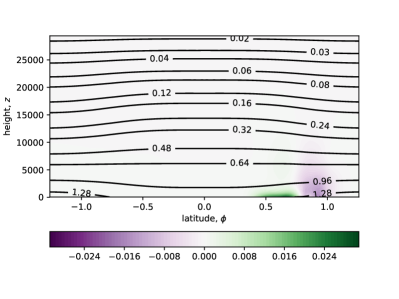
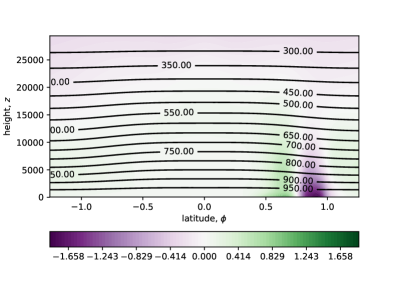
Figure 1: Baroclinic instability test case: Zonal averages of density, $\rho_{h}$ in $\mathrm{kg}\cdot\mathrm{m}^{-3}$ (left) and Exner pressure, $\Pi_{h}$ in $\mathrm{m}^{2}\mathrm{s}^{-2}\mathrm{K}^{-1}$ (right) at day 10. Contours represent absolute values, and shades represent differences from initial values.

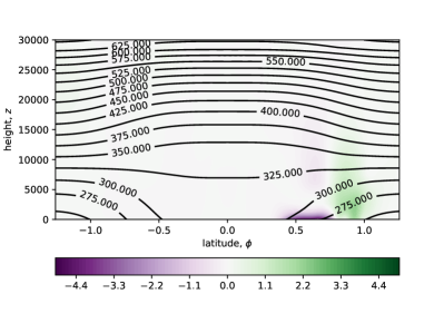
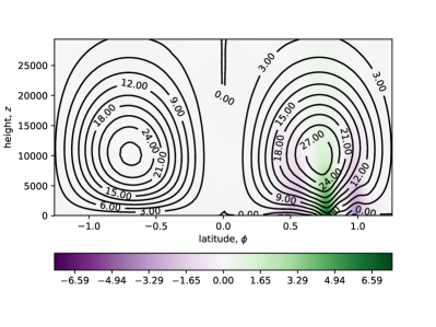
Figure 2: Baroclinic instability test case: Zonal averages of potential temperature, $\theta_{h}$ in $\mathrm{K}$ (left) and zonal velocity, $u_{h}$ in $\mathrm{m}\cdot\mathrm{s}^{-1}$ (right) at day 10. Contours represent absolute values, and shades represent differences from initial values.

Figure 3 shows the evolution of the potential, internal and kinetic (horizontal and vertical) energy with time. As can be seen the advent of the baroclinic instability coincides with a loss of both potential and internal energy, and an increase of kinetic energy due to acceleration in both the horizontal and vertical directions. The signature of the internal gravity waves is also visible in the smaller scale oscillation of the potential and horizontal kinetic energies. Note that the total amounts of potential and internal energy are approximately $3.6\times 10^{23}$ and $9.2\times 10^{23}\mathrm{kg\cdot m^{2}s^{-2}}$ respectively, and so are several orders of magnitude greater than the amounts of horizontal and vertical kinetic energy (approximately $4.0\times 10^{20}$ and $3.0\times 10^{13}\mathrm{kg\cdot m^{2}s^{-2}}$ respectively). As such the flattening of the density contours from which the baroclinic instability draws energy are barely evident in Fig. 1.

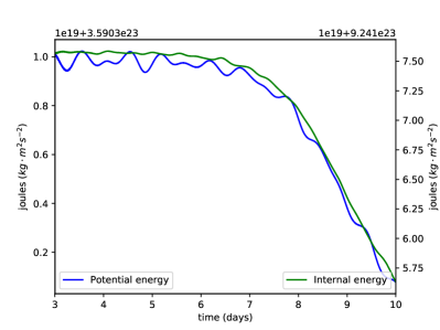
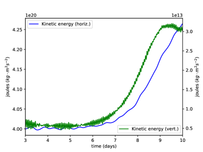
Figure 3: Baroclinic instability test case: Left: time evolution of the potential and internal energies. Right: time evolution of the kinetic energy (horizontal and vertical).

Figure 4 shows the power exchanges between kinetic, potential and internal energy, as given in (44)-(46). The evolution of the baroclinic instability is evident in the increase of power associated with the internal to horizontal kinetic energy exchanges. This figure also shows the typical convergence of the iterative solver with Newton iteration (taken at day 9). As can be seen, the convergence is poor for the first couple of Newton iterations, and the convergence of the velocity lags the other variables. After the first couple of iterations, the convergence improves, and reduces the errors between one and two decades at each iteration. Note that as the Jacobian is only approximate, we do not anticipate the convergence to be strictly quadratic. Also note that this convergence plot shows the convergence for the column of elements with the largest error, which may not necessarily be the same column between Newton iterations.

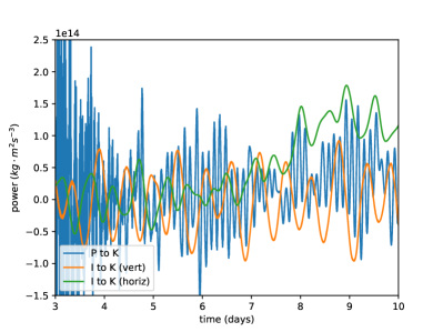
Figure 4: Baroclinic instability test case: Left: power associated with energetic exchanges, days 3 to 10. Right: typical convergence of the normalised $L^{2}$ magnitude of the solution updates with Newton iteration (taken at day 9).

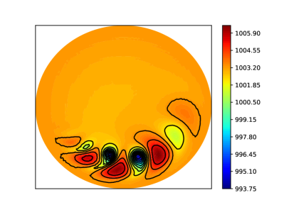
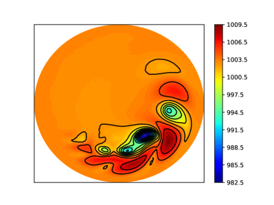
Figure 5: Baroclinic instability test case: Bottom level Exner pressure, $\Pi_{h}$ (in $\mathrm{hPa}$) day 8 (left) and 10 (right).

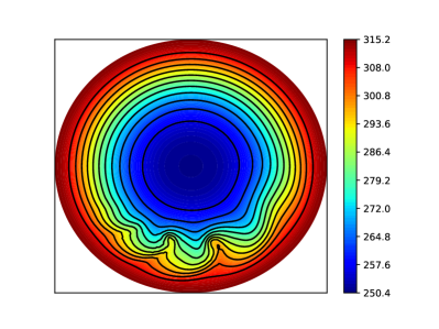
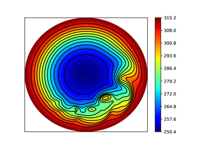
Figure 6: Baroclinic instability test case: Potential temperature, $\theta_{h}$ (in ${}^{\circ}\mathrm{K}$) at $z\approx 1.5\mathrm{km}$, day 8 (left) and 10 (right).

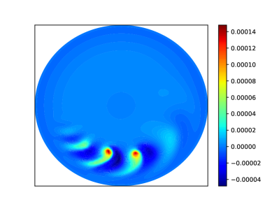
Figure 7: Baroclinic instability test case: Vertical component of the relative vorticity, $\omega_{h}$ (in $\mathrm{s}^{-1}$) at $z\approx 1.5\mathrm{km}$, day 8 (left) and 10 (right).

The bottom level Exner pressure $\Pi$, potential temperature, $\theta$, and the vertical component of the relative vorticity, $\omega$ are presented for $z\approx 1.5\mathrm{km}$ at days $8$ and $10$ in Figs. 5, 6 and 7, and the meridional cross section of the pressure perturbation at $50^{\circ}\mathrm{N}$ is given in Fig. 8. In the cases of the pressure, this is reconstructed from the model variables as $p=p_{0}(\Pi/c_{p})^{c_{p}/R}$. The pressure perturbation in Fig. 8 is then derived by removing the average pressure at the corresponding vertical level at $50^{\circ}\mathrm{S}$. These results compare well with the previously published test case results [34], and the vertical pressure perturbation profile exhibits less noise than the previous version of the implicit solver [8].

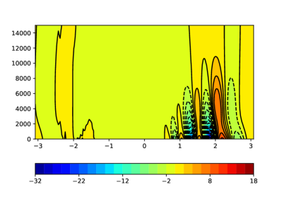
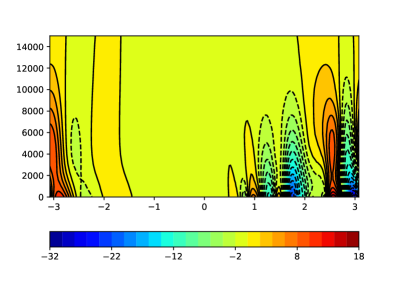
Figure 8: Baroclinic instability test case: Vertical cross section of the pressure perturbation, $p_{h}-\bar{p}_{h}$ (in $\mathrm{hPa}$) at $50^{\circ}\mathrm{N}$, day 8 (left) and day 10 (right).

In order to validate the conservation properties of the implicit solver the horizontal dynamics were turned off and the model was re-run with only the implicit vertical solver active (such that the horizontal velocity was not updated between time steps), and all the dissipation terms removed. Note that while the horizontal scheme conserves mass [8], it does not conserve energy due to the explicit time integration. As shown in Fig. 9 while the mass is conserved to machine precision, the conservation of energy is satisfied only for a solver tolerance below approximately $10.0^{-12}$. For tolerances greater than this a small drift in energy conservation is observed.

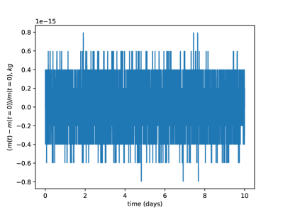
Figure 9: Baroclinic instability test case (vertical dynamics only): Global conservation errors for mass (left) and total energy as a function of solver tolerance (right).

Figure 10 shows the number of nonlinear iterations required to achieve convergence as a function of solver tolerance (again with the horizontal dynamics disabled). Note that the vertical velocity error has been removed from the set of convergence criteria, since the vertical kinetic energy is extremely small compared to the amounts of potential and internal energy, and the vertical velocity convergence error lags that of the other solution variables, as shown in Fig. 4. As can be observed the number of iterations increases somewhat linearly with solver tolerance at a rate of approximately one iteration per decade. Note that the Jacobian as detailed in (49) and (50) is only approximate, so quadratic convergence is not anticipated.

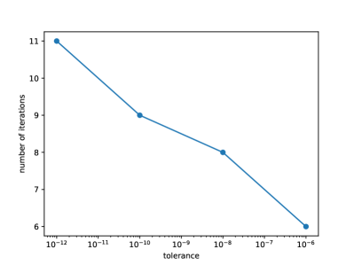
Figure 10: Baroclinic instability test case (vertical dynamics only): Number of nonlinear iterations to reach convergence as function of solver tolerance.

The energy conservation errors in Fig. 9 are compared to those for the standard Crank-Nicolson semi-implicit integrator as used in each vertical sub-step of the original TRAP(2,3,2) scheme [9, 10]. The Crank-Nicolson scheme is reverse-engineered from the existing energetically balanced scheme by removing all of the cross terms between time level $n$ and Newton iteration $k$ as given in (48), (41), and weighting the system at time levels $n$ and $k$ as $0.5$. All other aspects of the code are un-modified, including the energetically balanced spatial discretisation [8], and in both cases a tolerance of $10^{-12}$ is used (with the vertical velocity again omitted from the convergence criteria).

As observed in Fig 11, if only the vertical dynamics are considered, then the energy conservation errors of the Crank-Nicolson scheme, while still small, are $\mathcal{O}(10^{4})$ times greater than those of the energetically balanced integrator. While the Crank-Nicolson scheme is known to be unconditionally stable, such that the energy conservation errors remain bounded, the exchanges in energy remain unbalanced, and there is a noticeable oscillation in total energy with a period of approximately 3.5 days. This is despite the fact that both schemes involve balanced energy exchanges within the spatial discretisation, and differ only in the evaluation of additional cross terms in the temporal discretisation. For the full three dimensional model, the Crank-Nicolson integrator exhibits greater oscillation in the energy conservation errors during the initial period of hydrostatic adjustment, however after this initial period the energy conservation errors are actually greater for the energetically balanced scheme. This is perhaps due to the inclusion of the Rayleigh damping term in the top three levels. The energetically balanced scheme is perhaps more efficient at transmitting waves to the top of the domain, where these motions are damped by Rayligh friction. Nevertheless the growth in energy conservation error is faster for the Crank-Nicolson scheme over this period. Over the course of the simulation both integrators tend towards the same conservation error (which is marginally lower for the energetically balanced scheme), suggesting that for long times horizontal dissipative terms that are the same in both models dominate the energy conservation error.

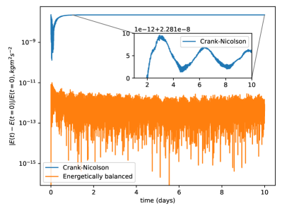
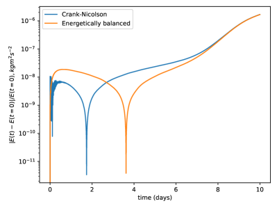
Figure 11: Baroclinic instability test case: Comparison of global energy conservation errors for the energetically balanced and standard Crank-Nicolson integrators, left: vertical dynamical only, right: full model (normalised absolute value of error).

6.2 Non-hydrostatic gravity wave

In order to validate the vertical integrator at high resolutions at which non-hydrostatic dynamics become significant the model has also been tested for the propagation of a non-hydrostatic gravity wave driven by a potential temperature perturbation on a planet with a reduced radius $125$ times smaller than that of the earth. This test was originally proposed as part of the 2012 DCMIP workshop [35], and specific details of the initial configuration can be found within the DCMIP test case document on the web site.

As for the baroclinic instability test, the simulation was run with a resolution of $24\times 24$ elements of degree $p=3$ in each cubed sphere panel. We use 16 evenly spaced vertical levels over a total height of $10,000.0$m, and a time step of $\Delta t=0.5$s for a total simulation time of $3600$s. In order to account for the highly oscillatory nature of the dynamics the horizontal biharmonic viscosity was rescaled by a factor of $2.0$ for both the momentum and temperature equations for a value of $0.144\Delta x^{3.2}$.

One particular challenge of this test case is the inexact integration of the horizontal metric terms on a planet of reduced radius. These terms include transcendental functions that cannot be integrated exactly [22, 17]. While the relative curvature of earth the with respect to the element size is small for the case of an earth of regular size, on an earth of reduced size under-integration of the metric terms may result in substantial aliasing errors that are not present in models based on polyhedral meshes.

Figure 12 shows the longitude-height equatorial ($\phi=0^{\circ}$) cross section of the potential temperature perturbation, $\theta^{\prime}(\lambda,0,z)=\theta(\lambda,0,z)-\bar{\theta}(z)$, where $\bar{\theta}(z)$ is the mean potential temperature at a given height, after 30 minutes and 1 hour. While the structure and evolution of the perturbation qualitatively match the results presented for other non-hydrostatic models, the results here are slightly more oscillatory than those of other models, perhaps reflecting the presence of aliasing errors due to the inexact integration of the metric terms on a planet of increased curvature. Moreover these results also show the ejection of a small hot bubble which rises to the top of the domain, which is also perhaps an artefact of the inexact spatial integration.

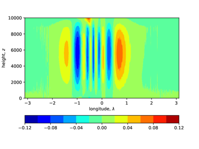
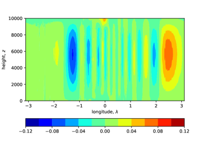
Figure 12: Non-hydrostatic gravity wave test case: Longitude-height equatorial ($\phi=0^{\circ}$) cross section of the potential temperature perturbation, $\theta^{\prime}(\lambda,0,z)=\theta(\lambda,0,z)-\bar{\theta}(z)$ at times $t=30$ minutes (left) and $t=60$ minutes (right).

The energy partitions are given for the final 12 minutes of the simulation in Fig. 13. The signature of the internal gravity wave is clearly visible in the oscillation between potential and internal energy. The horizontal dynamics are also observed in the longer time scale oscillation of kinetic to internal energy exchanges. This is also observed in the power exchanges as given in Fig. 14.

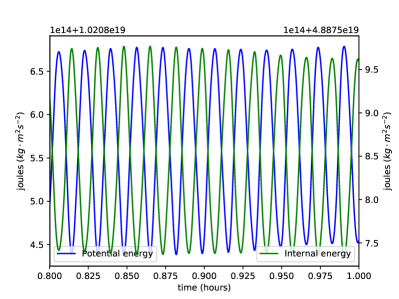
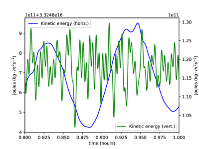
Figure 13: Non-hydrostatic gravity wave test case: Internal gravity wave; left: time evolution of the potential and internal energies, right: time evolution of the kinetic energy (horizontal and vertical).

Figure 14 also shows nonlinear convergence of the vertical solver at time $t=1$ hour. Due to the more regular vertical structure than the baroclinic test case the convergence of the nonlinear solver is faster and more regular, taking just 4 iterations.

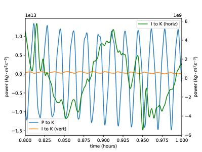
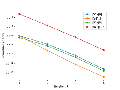
Figure 14: Non-hydrostatic gravity wave test case: Left: power associated with energetic exchanges, days 3 to 10. Right: typical convergence of the normalised $L^{2}$ magnitude of the solution updates with Newton iteration (at 1 hour).

Figure 15 shows the energy conservation errors for the non-hydrostatic gravity wave test case using both the energetically balanced and Crank-Nicolson vertical integrators. There is little difference between the errors for the two different vertical integrators, which are due to the horizontal dissipation terms, or indeed the time variation in kinetic, potential or internal energy (not shown). However over the course of the simulation a significant difference develops in the vertical kinetic to internal energy exchange. This does not seem to have an appreciable impact on the dynamics over the course of the simulation, but may possibly become significant over longer simulations.

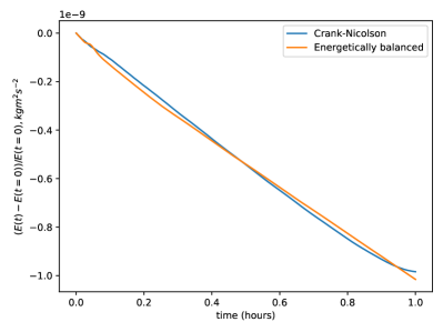
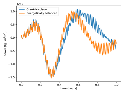
Figure 15: Non-hydrostatic gravity wave test case: comparisons of energetically balanced to Crank-Nicolson vertical integrator, energy conservation errors (left) and vertical internal to kinetic energy exchanges (right).

6.3 3D rising bubble

The model is further validated for the case of a 3D rising bubble of potential temperature within a high resolution Cartesian geometry. This involves re-configuring the model geometry as a single panel on a flat surface with periodic boundaries, while retaining the original boundary conditions in the vertical dimension. The test is performed within a high resolution domain of size $1000.0\mathrm{m}\times 1000.0\mathrm{m}\times 1500.0\mathrm{m}$ using $24\times 24$ elements of degree $p=3$ in the horizontal and 150 elements of degree $p=1$ in the vertical and a time step of $\Delta t=0.02\mathrm{s}$ in order to resolve the horizontal sound waves. The dissipation terms and coefficients are identical to those used in the non-hydrostatic gravity wave test case (biharmonic viscosity applied to the horizontal momentum and potential temperature advection equations, and no dissipation of any kind applied to the vertical dynamics). Notably there is no upwinding or viscosity within the vertical system, so there is nothing to prevent overshoots or oscillations as the gradient of the bubble steepens.

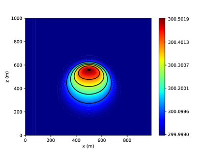
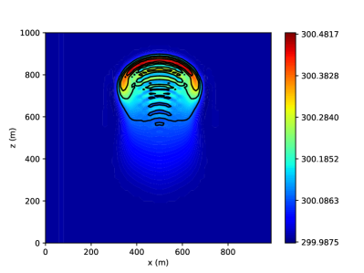
Figure 16: 3D rising bubble test case: potential temperature, $\theta_{h}$, cross section at $y=500.0\mathrm{m}$ at time $200.0\mathrm{s}$ (left) and time $400.0\mathrm{s}$ (right). Contours are from $300.1^{\circ}\mathrm{K}$ to $300.5^{\circ}\mathrm{K}$ in increments of $0.1^{\circ}\mathrm{K}$.

The bubble is initialised against a constant background state of $\theta_{0}=300.0^{\circ}\mathrm{K}$ as $\theta^{\prime}=0.25(1.0+\cos(\pi r/r_{0}))$ for $r\leq r_{0}$, where $r=\sqrt{(x-250.0)^{2}+(y-250.0)^{2}+(z-350.0)^{2}}$ and $r_{0}=250.0$ [12], and the Exner pressure is initialised from a state of hydrostatic balance as $\Pi=c_{p}(1-gz/c_{p}\theta_{0})$ [36]. The initial density is then derived via the equation of state (3). The position, deformation and amplitude of the bubble compare well to previous results [25, 12], as observed in Fig. 16. However the absence of any viscous or upwinding terms from the vertical discretisation ensures that as the bubble ascends a spurious oscillation develops within its wake, and the amplitude of the disturbance is not strictly monotone. In order to suppress this oscillation some form of vertical upwinding should be implemented, as is the case in other non-hydrostatic models [12, 4].

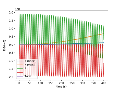
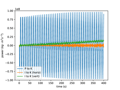
Figure 17: 3D rising bubble test case: variation in energy from initial state (left) and power exchanges (right).

Figure 17 details the energy variation and power exchanges with time for the rising bubble. In addition to the steady decrease in potential energy and increase in vertical kinetic energy as the bubble rises, these clearly show the signature of an internal gravity wave of period approximately $8\mathrm{s}$ that oscillates within the domain. The vertical integrator takes just three iterations to converge for the rising bubble test case (with the vertical velocity removed from the list of convergence criteria, since the bubble is initially at rest). This is perhaps because the aspect ratio between the horizontal and vertical scales is unity, such that the requirement that the horizontal acoustic modes be resolved in time implies that the vertical modes are resolved also.

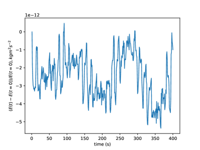
Figure 18: 3D rising bubble test case (vertical dynamics only): Global total energy conservation error.

In order to further validate the energy conservation of the new integrator the 3D rising bubble test case is run with the vertical dynamics only. Since this test is run on a planar geometry, there is no aliasing error associated with the inexact integration of transcendental metric terms, as is the case for the spherical geometry. While the dynamics are compressible, the ascension of the bubble occurs primarily in the incompressible regime, so only the gravity and acoustic modes are discernible without horizontal motions. Without horizontal acoustic modes, the code can be run with a greatly increased time step, and here we use a step size of $\Delta t=1s$, as well as $4\times 4$ elements of degree $p=3$ at each of the $150$ vertical levels, and no horizontal variation in the initial condition. As observed in Fig. 18 the energy conservation errors are comparable to those for the planetary configuration as given in Fig. 9, for which both the metric terms and the vertical structure are more complex.

The differences between the energetics using the energetically balanced and Crank-Nicolson vertical integrator have also been compared for the 3D rising bubble test case (not shown). Owing to the small time step required to resolve the horizontal sound waves (which is the same as the time scale for the vertical sound waves), and the simple vertical structure of this test case, the differences between the energetics for the two vertical integrators are marginal and only barely perceptible.

7 Conclusions

An energetically balanced time integrator for vertical atmospheric dynamics is presented. The integrator balances energetic exchanges associated with vertical motions by preserving the skew-symmetric property of the non-canonical Hamiltonian form of the compressible Euler equations in space and and the exact integration of the variational derivatives on the Hamiltonian in time. The computational efficiency of the integrator is accelerated via a reduction of the four component system to a single equation for the density weighted potential temperature at each nonlinear iteration. The integrator is implemented within the context of a horizontally explicit/vertically implicit scheme in which the vertical time stepping is centered so as to allow for second order accuracy and exact integration in time. The integrator demonstrates robust convergence at both global and non-hydrostatic resolutions.

In future work the issue of the time splitting error associated with the density and density weighted potential temperature fluxes will be addressed. These can most likely be reformulated so as to suppress this error and ensure consistency between time levels. A full three dimensional version of the implicit integrator will also be investigated, and further examinations between the energetically balanced formulation and existing schemes will be explored.

8 Acknowledgments

David Lee would like to thank Drs. Marcus Thatcher and John McGregor for their continued support and access to computing resources. This project was supported by resources and expertise provided by CSIRO IMT Scientific Computing.

References

• [1] W. Bauer, C. J. Cotter, Energy-enstrophy conserving compatible finite element schemes for the rotating shallow water equations with slip boundary conditions, J. Comp. Phys. 373 (2018) 171–187.
• [2] G. A. Wimmer, C.J. Cotter, W. Bauer, Energy conserving upwinded compatible finite element schemes for the rotating shallow water equations, J. Comp. Phys. 401 (2020) 109016
• [3] C. Eldred, T. Dubos, E. Kritsikis, A quasi-Hamiltonian discretization of the thermal shallow water equations, J. Comp. Phys. 379 (2019) 1–31.
• [4] G. A. Wimmer, C.J. Cotter, W. Bauer, Energy conserving SUPG methods for compatible finite element schemes in numerical weather prediction, arXiv:2001.09590 (2020)
• [5] K. Kormann, E. Sonnendrücker, Energy-conserving time propagation for a geometric particle-in-cell Vlasov–Maxwell solver, arXiv:1910.04000 (2019)
• [6] R. I. McLachlan, G. R. W. Quispel, N. Robidoux, Geometric integration using discrete gradients, Phil. Trans. R. Soc. A 357 (1999) 1021–1046.
• [7] D. Cohen, E. Hairer, Linear energy-preserving integrators for Poisson systems, BIT Numer. Math. 51 (1) (2011) 91–101.
• [8] D. Lee, A. Palha, A mixed mimetic spectral element model of the 3D compressible Euler equations on the cubed sphere, J. Comp. Phys. 401 (2020) 108993
• [9] H. Weller, S. J. Lock, N. Wood, Runge–Kutta IMEX schemes for the Horizontally Explicit/Vertically Implicit (HEVI) solution of the wave equations, J. Comp. Phys. 252 (2013) 365–381.
• [10] S.-J. Lock, N. Wood, H. Weller, Numerical analyses of Runge–Kutta implicit–explicit schemes for horizontally explicit, vertically implicit solutions of atmospheric models, Q. J. R. Meteorol. Soc. 140 (2014) 1654–1669.
• [11] M. A. Taylor, O. Guba, A. Steyer, P. A. Ullrich, D. M. Hall, C.Eldred, An Energy Consistent Discretization of the Nonhydrostatic Equations in Primitive Variables, JAMES, 12 (2020) 1–20.
• [12] T. Melvin, T. Benacchio, B. Shipway, N. Wood, J. Thuburn, C. Cotter, A mixed finite-element, finite-volume, semi-implicit discretisation for atmospheric dynamics: Cartesian geometry, Q. J. R. Meteorol. Soc. (2019) 1–19.
• [13] C. Maynard, T. Melvin, E. H. Müller, Performance of multigrid solvers for the mixed finite element dynamical core LFRic, arXiv:2002.00756, (2020)
• [14] M. Gerritsma, Edge functions for spectral element methods, in: Spectral and high order methods for partial differential equations, Lecture Notes in Computational Science and Engineering, Springer 76 (2011) 199–207.
• [15] J. Kreeft, M. Gerritsma, Mixed mimetic spectral element method for Stokes flow: A pointwise divergence-free solution, J. Comp. Phys. 240 (2013) 284–309.
• [16] D. Lee, A. Palha, M. Gerritsma, Discrete conservation properties for shallow water flows using mixed mimetic spectral elements, J. Comp. Phys. 357 (2018) 282–304.
• [17] D. Lee, A. Palha, A mixed mimetic spectral element model of the rotating shallow water equations on the cubed sphere, J. Comp. Phys. 375 (2018) 240–262.
• [18] P. Névir, M. Sommer, Energy-vorticity theory of ideal fluid mechanics, J. Atmos. Sci. 66 (2009) 2073–2084.
• [19] A. Gassmann, A global hexagonal C‐grid non‐hydrostatic dynamical core (ICON‐IAP) designed for energetic consistency, Q. J. R. Meteorol. Soc. 139 (2013) 152–175.
• [20] A. A. White, B. J. Hoskins, I. Roulstone, A. Staniforth, Consistent approximate models of the global atmosphere: shallow, deep, hydrostatic, quasi-hydrostatic and non-hydrostatic, Q. J. R. Meteorol. Soc. 131 (2005) 2081–2107.
• [21] E. Hairer, C. Lubich, G. Wanner, Geometric Numerical Integration, Springer, 2006.
• [22] O. Guba, M. A. Taylor, P. A. Ullrich, J. R. Overfelt, M. N. Levy, The spectral element method (SEM) on variable-resolution grids: evaluating grid sensitivity and resolution-aware numerical viscosity, Geosci. Model. Dev. 7 (2014) 2803–2816.
• [23] E. Celledoni, V. Grimm, R. I. McLachlan, D. I. McLaren, D. O’Neale, B. Owren, G. R. W. Quispel, Preserving energy resp. dissipation in numerical PDEs using the ”average vector field” method, J. Comp. Phys. 231 (2012) 6770–6789.
• [24] P. Ullrich, C. Jablonowski, Operator-split Runge–Kutta–Rosenbrock methods for nonhydrostatic atmospheric models, Mon. Wea. Rev. 140 (2012) 1257–1284.
• [25] F. X. Giraldo, J. F. Kelly, E. M. Constantinescu, Implicit-explicit formulations of a three-dimensional nonhydrostatic unified model of the atmosphere (NUMA), SIAM J. Sci. Comput. 35 (2013) B1162–B1194.
• [26] L. Bao, R. Klöfkorn, R. D. Nair, Horizontally explicit and vertically implicit (HEVI) time discretization scheme for a discontinuous Galerkin nonhydrostatic model, Mon. Wea. Rev. 143 (2015) 972–990.
• [27] D. J. Gardner, J. E. Guerra, F. P. Hamon, D. R. Reynolds, P. A. Ullrich, C. S. Woodward, Implicit-explicit (IMEX) Runge-Kutta methods for non-hydrostatic atmospheric models, Geosci. Model Dev. 11 (2018) 1497–1515.
• [28] A. Natale, J. Shipton, C. J. Cotter, Compatible finite element spaces for geophysical fluid dynamics, Dyn. Stat. Climate Sys. 1 (2016) 1–31.
• [29] J. M. Reisner, V. A. Mousseau, A. A. Wyszogrodzki, D. A. Knoll, An Implicitly Balanced Hurricane Model with Physics-Based Preconditioning, Mon. Wea. Rev. 133 (2005) 1003–1022.
• [30] S. Balay, S. Abhyankar, M. F. Adams, J. Brown, P. Brune, K. Buschelman, L. Dalcin, V. Eijkhout, W. D. Gropp, D. Kaushik, M. G. Knepley, D. A. May, L. C. McInnes, K. Rupp, B. F. Smith, S. Zampini, H. Zhang, PETSc Web page, http://www.mcs.anl.gov/petsc (2017).
• [31] S. Balay, S. Abhyankar, M. F. Adams, J. Brown, P. Brune, K. Buschelman, L. Dalcin, V. Eijkhout, W. D. Gropp, D. Kaushik, M. G. Knepley, D. A. May, L. C. McInnes, K. Rupp, P. Sanan, B. F. Smith, S. Zampini, H. Zhang, PETSc users manual, Tech. Rep. ANL-95/11 - Revision 3.8, Argonne National Laboratory (2017).
• [32] S. Balay, W. D. Gropp, L. C. McInnes, B. F. Smith, Efficient management of parallelism in object oriented numerical software libraries, in: E. Arge, A. M. Bruaset, H. P. Langtangen (Eds.), Modern Software Tools in Scientific Computing, Birkhäuser Press, 1997, pp. 163–202.
• [33] J. B. Klemp, J. Dudhia, A. D. Hassiotis, An upper gravity-wave absorbing layer for NWP applications, Mon. Wea. Rev. 136 (2008) 3987–4004.
• [34] P. A. Ullrich, T. Melvin, C. Jablonowski, A. Staniforth, A proposed baroclinic wave test case for deep‐ and shallow‐atmosphere dynamical cores, Q. J. R. Meteorol. Soc. 140 (2014) 1590–1602.
• [35] C. Jablonowski, P. A. Ullrich, J. Kent, K. Reed, M. A. Taylor, P. H. Lauritzen, R. D. Nair, DCMIP 2012 test case 3.1, https://www.earthsystemcog.org/projects/dcmip-2012/test_cases (2012).
• [36] D. S. Abdi, F. X. Giraldo, Efficient construction of unified continuous and discontinuous Galerkin formulations for the 3D Euler equations, J. Comp. Phys. 320 (2016) 46–68