A cross-product free Jacobi-Davidson type method for computing a partial generalized singular value decomposition of a large matrix pair

Abstract

A Cross-Product Free (CPF) Jacobi-Davidson (JD) type method is proposed to compute a partial generalized singular value decomposition (GSVD) of a large regular matrix pair $(A,B)$. It implicitly solves the mathematically equivalent generalized eigenvalue problem of $(A^{T}A,B^{T}B)$ but does not explicitly form the cross-product matrices and thus avoids the possible accuracy loss of the computed generalized singular values and generalized singular vectors. The method is an inner-outer iteration method, where the expansion of the right searching subspace forms the inner iterations that approximately solve the correction equations involved and the outer iterations extract approximate GSVD components with respect to the subspaces. Some convergence results are established for the inner and outer iterations, based on some of which practical stopping criteria are designed for the inner iterations. A thick-restart CPF-JDGSVD algorithm with deflation is developed to compute several GSVD components. Numerical experiments illustrate the efficiency of the algorithm.

1 Introduction

The generalized singular value decomposition (GSVD) of a matrix pair is first introduced by Van Loan [28] and then developed by Paige and Saunders [22]. It has become an important analysis means and computational tool [9], and has been used extensively in, e.g., solutions of discrete linear ill-posed problems [12], weighted or generalized least squares problems [3], information retrieval [14], linear discriminant analysis [23], and many others [2, 4, 9, 21, 27].

Let $A\in\mathbb{R}^{m\times n}$ and $B\in\mathbb{R}^{p\times n}$ with $m\geq n$ be large matrices, and assume that the stacked matrix $\begin{bmatrix}\begin{smallmatrix}A\\ B\end{smallmatrix}\end{bmatrix}$ has full column rank, i.e., $\mathcal{N}(A)\cap\mathcal{N}(B)=\{\mathbf{0}\}$ with $\mathcal{N}(A)$ and $\mathcal{N}(B)$ the null spaces of $A$ and $B$, respectively. Then such matrix pair $(A,B)$ is called regular. Denote $q_{1}=\dim(\mathcal{N}(A))$ and $q_{2}=\dim(\mathcal{N}(B))$, $q=n-q_{1}-q_{2}$, and $l_{1}=\dim(\mathcal{N}(A^{T}))$ and $l_{2}=\dim(\mathcal{N}(B^{T}))$. Then the GSVD of the regular matrix pair $(A,B)$ is

(1.1) $$\left\{\begin{aligned} &U^{T}AX=\Sigma_{A}=\mathop{\operator@font diag}\nolimits\{C,\mathbf{0}_{l_{1},q_{1}},I_{q_{2}}\},\\ &V^{T}BX=\Sigma_{B}=\mathop{\operator@font diag}\nolimits\{S,I_{q_{1}},\mathbf{0}_{l_{2},q_{2}}\},\end{aligned}\right.$$

where $X=[X_{q},X_{q_{1}},X_{q_{2}}]$ is nonsingular, $U=[U_{q},U_{l_{1}},U_{q_{2}}]$ and $V=[V_{q},V_{q_{1}},V_{l_{2}}]$ are orthogonal, and $C=\mathop{\operator@font diag}\nolimits\{\alpha_{1},\dots,\alpha_{q}\}$ and $S=\mathop{\operator@font diag}\nolimits\{\beta_{1},\dots,\beta_{q}\}$ are diagonal matrices that satisfy

$$0<\alpha_{i},\beta_{i}<1\quad\mbox{and}\quad\alpha_{i}^{2}+\beta_{i}^{2}=1,\quad i=1,\dots,q;$$

see [22]. Here, in order to distinguish the block submatrices of $X,U,V$, we have adopted the subscripts to denote their column and row numbers, and have denoted by $I_{k}$ and $\mathbf{0}_{k,l}$ the identity matrix of order $k$ and zero matrix of order $k\times l$, respectively. The subscripts of identity and zero matrices will be omitted in the sequel when their orders are clear from the context. It follows from (1.1) that $X^{T}(A^{T}A+B^{T}B)X=I_{n}$, i.e., the columns of $X$ are $(A^{T}A+B^{T}B)$-orthonormal.

The GSVD components $(\mathbf{0}_{l_{1},q_{1}},I_{q_{1}},U_{l_{1}},V_{q_{1}},X_{q_{1}})$ and $(I_{q_{2}},\mathbf{0}_{l_{2},q_{2}},U_{q_{2}},V_{l_{2}},X_{q_{2}})$ are associated with the zero and infinite generalized singular values of $(A,B)$, called the trivial ones, and the columns of $U_{l_{1}}$, $V_{l_{2}}$ and $X_{q_{1}}$, $X_{q_{2}}$ form orthonormal and $(A^{T}A+B^{T}B)$-orthonormal bases of $\mathcal{N}(A^{T})$, $\mathcal{N}(B^{T})$ and $\mathcal{N}(A)$, $\mathcal{N}(B)$, respectively. Denote by $u_{i},v_{i}$ and $x_{i}$ the $i$-th columns of $U_{q}$, $V_{q}$ and $X_{q}$, respectively, $i=1,\dots,q.$ The quintuple $(\alpha_{i},\beta_{i},u_{i},v_{i},x_{i})$ is called a nontrival GSVD component of $(A,B)$ with the generalized singular value $\sigma_{i}=\frac{\alpha_{i}}{\beta_{i}}$, the left generalized singular vectors $u_{i}$, $v_{i}$ and the right generalized singular vector $x_{i}$. We also refer to a pair $(\alpha_{i},\beta_{i})$ as a generalized singular value of $(A,B)$.

For a given target $\tau>0$, assume that the nontrivial generalized singular values $\sigma_{i},\,i=1,2,\ldots,q$ of $(A,B)$ are labeled as

(1.2) $$|\sigma_{1}-\tau|\leq|\sigma_{2}-\tau|\leq\dots\leq|\sigma_{\ell}-\tau|<|\sigma_{\ell+1}-\tau|\leq\dots\leq|\sigma_{q}-\tau|.$$

We are interested in computing the $\ell$ GSVD components $(\alpha_{i},\beta_{i},u_{i},v_{i},x_{i})$ corresponding to the generalized singular values closest to $\tau$. If $\tau$ is inside the spectrum of the nontrivial generalized singular values of $(A,B)$, then $(\alpha_{i},\beta_{i},u_{i},v_{i},x_{i})$, $i=1,\dots,\ell$, are called interior GSVD components of $(A,B)$; otherwise, they are called the extreme, i.e., largest or smallest, ones. A large number of GSVD components, i.e., $\ell\gg 1$, some of which are interior ones, may be required in applications, including nonlinear dimensionality reduction and data science [5, 6, 7]. Without loss of generality, we always assume that $\tau$ is not equal to any generalized singular value of $(A,B)$.

Zha [29] proposes a joint bidiagonalization (JBD) method for computing extreme GSVD components of the large matrix pair $(A,B)$. At each step of JBD, one needs to solve an $(m+p)\times n$ least squares problem with the coefficient matrix $\begin{bmatrix}\begin{smallmatrix}A\\ B\end{smallmatrix}\end{bmatrix}$, which may be costly using an iterative solver [20]. Hochstenbach [13] presents a Jacobi–Davidson (JD) type GSVD (JDGSVD) method to compute $\ell$ GSVD components of $(A,B)$ with the full column rank $B$, where, at each expansion step, a correction equation of dimension $m+n$ needs to be solved iteratively with low or modest accuracy; see [15, 17, 18]. The upper $m$-dimensional part and the lower $n$-dimensional part of the approximate solution are used to expand one of the left searching subspaces and the right searching subspace. The JDGSVD method formulates the GSVD of $(A,B)$ as the mathematically equivalent generalized eigendecomposition of the augmented matrix pair $\left(\begin{bmatrix}\begin{smallmatrix}&A\\ A^{T}&\end{smallmatrix}\end{bmatrix},\begin{bmatrix}\begin{smallmatrix}I&\\ &B^{T}B\end{smallmatrix}\end{bmatrix}\right)$ for the full column rank $B$ (resp. $\left(\begin{bmatrix}\begin{smallmatrix}&B\\ B^{T}&\end{smallmatrix}\end{bmatrix},\begin{bmatrix}\begin{smallmatrix}I&\\ &A^{T}A\end{smallmatrix}\end{bmatrix}\right)$ for the full column rank $A$), computes the relevant eigenpairs and recovers the approximate GSVD components from the converged eigenpairs.

The side effects of involving the cross-product matrix $B^{T}B$ in JDGSVD method are twofold. First, in the extraction phase, one is required to compute a $B^{T}B$-orthonormal basis of the right searching subspace, which is numerically unstable when $B$ is ill conditioned. Second, it is shown in [16] that the error of the computed eigenvector is bounded by the size of the perturbations times a multiple $\kappa(B^{T}B)=\kappa^{2}(B)$, where $\kappa(B)=\sigma_{\max}(B)/\sigma_{\min}(B)$ denotes the $2$-norm condition number of $B$ with $\sigma_{\max}(B)$ and $\sigma_{\min}(B)$ being the largest and smallest singular values of $B$, respectively. Consequently, with an ill-conditioned $B$, the computed GSVD components may have very poor accuracy and has been numerically confirmed [16]. We remark that all the eigenvalue-based type GSVD methods share this shortcoming of JDGSVD. The results in [16] show that if $B$ is ill conditioned but $A$ has full column rank and is well conditioned then the JDGSVD method can be applied to the matrix pair $(B,A)$ and compute the corresponding approximate GSVD component with high accuracy [16]. However, a reliable estimation of the condition numbers of $A$ and $B$ is numerically challenging and may be costly. As a result, it is difficult to choose a proper formulation in applications.

Zwaan and Hochstenbach [31] present a generalized Davidson (GDGSVD) method and a multidirectional (MDGSVD) method, which are designed to compute an extreme partial GSVD of $(A,B)$. The methods avoid any cross product or matrix-matrix product by applying the standard extraction approach to $(A,B)$ directly for computing approximate GSVD components with respect to the given left and right searching subspaces with the two left subspaces formed by premultiplying the right subspace with $A$ and $B$, respectively. At each iteration of the GDGSVD method, the right searching subspace is spanned by the residuals of the generalized Davidson method [1, Sec. 11.2.4 and Sec. 11.3.6] applied to the generalized eigenvalue problem of $(A^{T}A,B^{T}B)$; in the MDGSVD method, a truncation technique is designed to discard an inferior search direction so as to improve the searching subspaces. Exploiting the Kronecker canonical form of a regular matrix pair [26], Zwaan [30] shows that the GSVD problem of $(A,B)$ can be formulated as a certain $(2m+p+n)\times(2m+p+n)$ generalized eigenvalue problem without using any cross product or any other matrix-matrix product. Currently, such formulation is of major theoretical value because the nontrivial eigenvalues and eigenvectors of the structured generalized eigenvalue problem are always complex with the generalized eigenvalues being the conjugate quaternions $(\sqrt{\sigma_{j}},-\sqrt{\sigma_{j}},\mathrm{i}\sqrt{\sigma_{j}},-\mathrm{i}\sqrt{\sigma_{j}})$ with $\mathrm{i}$ the imaginary unit and the associated right generalized eigenvectors being

$$[u_{j}^{T},x_{j}^{T}/\beta_{j},\sqrt{\sigma_{j}}u_{j}^{T},\sqrt{\sigma_{j}}v_{j}^{T}]^{T},\ [-u_{j}^{T},-x_{j}^{T}/\beta_{j},\sqrt{\sigma_{j}}u_{j}^{T},\sqrt{\sigma_{j}}v_{j}^{T}]^{T},$$

$$[-\mathrm{i}u_{j}^{T},\mathrm{i}x_{j}^{T}/\beta_{j},\sqrt{\sigma_{j}}u_{j}^{T},-\sqrt{\sigma_{j}}v_{j}^{T}]^{T},\ [\mathrm{i}u_{j}^{T},\mathrm{i}x_{j}^{T}/\beta_{j},-\sqrt{\sigma_{j}}u_{j}^{T},-\sqrt{\sigma_{j}}v_{j}^{T}]^{T}.$$

As is clear, the size of the generalized eigenvalue problem is much bigger than that of the GSVD of $(A,B)$. It is also unclear what the conditioning of eigenvalues and eigenvectors of this problem is. Furthermore, there has been no structure-preserving algorithm for the complicated structured generalized eigenvalue problem in [30]. It will be extremely difficult and highly challenging to seek for a numerically stable structure-preserving efficient algorithm for that structured generalized eigenvalue problem.

In order to compute GSVD components accurately, it is appealing to propose and develop algorithms that work on $A$ and $B$ directly. In this paper, we first propose a basic Cross-Product Free (CPF) JD type method for computing one, i.e., $\ell=1$, GSVD component of $(A,B)$, which is referred to as CPF-JDGSVD in the sequel. As done in the GDGSVD and MDGSVD methods [31], instead of constructing left and right searching subspaces separately or independently, given a right searching subspace, the CPF-JDGSVD method generates the corresponding two left searching subspaces by acting $A$ and $B$ on the right subspace, respectively, and constructs their orthonormal bases by computing two thin QR factorizations of the matrices that are formed by premultiplying the matrix consisting of the orthonormal basis vectors of the right subspace with $A$ and $B$, respectively. But unlike [31], at the extraction stage, our method projects the GSVD of $(A,B)$ onto the left and right searching subspaces without involving $A^{T}A$ and $B^{T}B$, and obtains an approximation to the desired GSVD component of $(A,B)$ by computing the GSVD of the small sized projection matrix pair. To be practical, we develop a thick-restart CPF-JDGSVD algorithm with deflation for computing several, i.e., $\ell>1$, GSVD components.

We shall, for the first time, give a theoretical justification that the left searching subspaces are as good as the right one as long as the desired generalized singular value $\sigma$ is not very small or large, that is, the distances of the desired left generalized singular vectors and the left subspaces are as small as that of the desired right generalized singular vector and the right subspace. We give a detailed derivation of certain new $n\times n$ correction equations involved in CPF-JDGSVD, whose solutions are exploited to expand right searching subspaces. The correction equations are supposed to be approximately solved iteratively, called inner iterations, and CPF-JDGSVD is an inner-outer iterative method with extraction steps of approximate GSVD components called outer iterations. We establish a convergence result on the approximate generalized singular values in terms of the residual norms. Meanwhile, we derive some results on the inner iterations in CPF-JDGSVD and obtain the asymptotic condition numbers of the correction equations. Based on them and analysis, we propose practical stopping criteria for the inner iterations, making the computational cost of the inner iterations minimal at each outer iteration and guarantee that CPF-JDGSVD behaves like the exact CPF-JDGSVD where the correction equations are solved exactly.

The rest of this paper is organized as follows. In Section 2, we propose the CPF-JDGSVD method and present some theoretical results on its rationale and convergence. In Section 3, we derive correction equations and establish some properties of them and some results on the inner iterations. Based on these results, we design practical stopping criteria for the inner iterations in CPF-JDGSVD. In Section 4, we propose a CPF-JDGSVD algorithm with restart and deflation for computing more than one GSVD components. Numerical experiments are reported in Section 5 to demonstrate the performance of CPF-JDGSVD and show its superiority to JDGSVD in [13] in terms of efficiency and accuracy. We should remind that, among the available algorithms, JDGSVD is the only available one that can be used to make a comparison with CPF-JDGSVD for computing the generalized singular values closest to a given target $\tau$. Finally, we conclude this paper in Section 6.

Throughout the paper, denote by $\|\cdot\|$ the $2$-norm of a vector or matrix, and assume that $\|A\|$ and $\|B\|$ themselves are modest, which can be achieved by suitable scaling. Since the stacked matrix $\begin{bmatrix}\begin{smallmatrix}A\\ B\end{smallmatrix}\end{bmatrix}$ is better and can be much better conditioned than both $A$ and $B$, we will assume that $\begin{bmatrix}\begin{smallmatrix}A\\ B\end{smallmatrix}\end{bmatrix}$ is well conditioned, which is definitely true, provided one of $A$ and $B$ is well conditioned.

2 The basic CPF-JDGSVD algorithm

We propose a basic CPF-JDGSVD method for computing one GSVD component $(\alpha,\beta,u,v,x):=(\alpha_{1},\beta_{1},u_{1},v_{1},x_{1})$ of $(A,B)$ corresponding to the generalized singular value $\sigma:=\sigma_{1}$ closest to the target $\tau$. The method includes three major ingredients: (i) the construction of left searching subspaces for a given right searching subspace, (ii) an extraction approach of approximate GSVD components, and (iii) an expansion approach of the right subspace. We will prove that the accuracy of the left searching subspaces constructed is similar to that of the right subspace, and will establish an important convergence result on the approximate generalized singular values.

2.1 Extraction approach

At iteration $k$, assume that a $k$-dimensional right searching subspace $\mathcal{X}$ is available, from which we seek an approximation to the right generalized singular vector $x$. For the left generalized singular vectors $u$ and $v$, since $Ax=\alpha u$ and $Bx=\beta v$, it is natural to construct $\mathcal{U}:=A\mathcal{X}$ and $\mathcal{V}:=B\mathcal{X}$ as left searching subspaces and seek approximations to $u$ and $v$ from them, respectively.

We shall present a theoretical justification that such $\mathcal{U}$ and $\mathcal{V}$ contain the same accurate information on the desired $u$ and $v$ as $\mathcal{X}$ does on $x$. As a result, it is possible to extract approximate left and right generalized singular vectors with similar accuracy.

Proposition 2.1.

Let $\mathcal{X}$ be a given right searching subspace and $\mathcal{U}=A\mathcal{X}$ and $\mathcal{V}=B\mathcal{X}$ be the left searching subspaces. Then for the desired right and left generalized singular vectors $x$ and $u$, $v$ of $(A,B)$ associated with the generalized singular value $\sigma=\frac{\alpha}{\beta}$ it holds that

(2.1) $$\sin\angle(\mathcal{U},u) \leq \frac{\|A\|\|x\|}{\alpha}\sin\angle(\mathcal{X},x),$$

(2.2) $$\sin\angle(\mathcal{V},v) \leq \frac{\|B\|\|x\|}{\beta}\sin\angle(\mathcal{X},x).$$

For an arbitrary vector $x^{\prime}\in\mathcal{X}$, by the definition of sine of the angle between arbitrary two nonzero vectors, we have

(2.3) $$\sin\angle(Ax^{\prime},Ax) = \min_{\mu}\frac{\|Ax-\mu Ax^{\prime}\|}{\|Ax\|}=\min_{\mu}\frac{\|A(x-\mu x^{\prime})\|}{\|Ax\|}$$

$$\leq \frac{\|A\|\|x\|}{\|Ax\|}\min_{\mu}\frac{\|x-\mu x^{\prime}\|}{\|x\|}$$

$$= \frac{\|A\|\|x\|}{\alpha}\sin\angle(x^{\prime},x),$$

where the last relation holds since $Ax=\alpha u$ with $\|u\|=1$. Therefore, we obtain

$$\sin\angle(\mathcal{U},u) = \sin\angle(A\mathcal{X},Ax)=\min_{x^{\prime}\in\mathcal{X}}\sin\angle(Ax^{\prime},Ax)$$

$$\leq \frac{\|A\|\|x\|}{\alpha}\min_{x^{\prime}\in\mathcal{X}}\sin\angle(x^{\prime},x)$$

$$= \frac{\|A\|\|x\|}{\alpha}\sin\angle(\mathcal{X},x),$$

i.e., relation (2.1) holds. (2.2) can be proved similarly.

Proposition 2.1 shows that when $\mathcal{X}$ contains good information on the desired $x$, the qualities of $\mathcal{U}$ and $\mathcal{V}$ are determined by $\alpha$, $\|A\|$, $\|x\|$, and by $\beta$, $\|B\|$, $\|x\|$, respectively. Since $\|X^{-1}\|^{-1}\leq\|x\|\leq\|X\|$, Theorem 2.3 in [11] states that

(2.4) $$\|X\|=\left\|\begin{bmatrix}\begin{smallmatrix}A\\ B\end{smallmatrix}\end{bmatrix}^{{\dagger}}\right\|\quad\mbox{and}\quad\|X^{-1}\|=\left\|\begin{bmatrix}\begin{smallmatrix}A\\ B\end{smallmatrix}\end{bmatrix}\right\|,$$

where ${\dagger}$ denotes the More-Penrose generalized inverse. Therefore, we have

(2.5) $$\left\|\begin{bmatrix}\begin{smallmatrix}A\\ B\end{smallmatrix}\end{bmatrix}\right\|^{-1}\leq\|x\|\leq\left\|\begin{bmatrix}\begin{smallmatrix}A\\ B\end{smallmatrix}\end{bmatrix}^{{\dagger}}\right\|.$$

By the assumption that $\begin{bmatrix}\begin{smallmatrix}A\\ B\end{smallmatrix}\end{bmatrix}$ is well conditioned and $\begin{bmatrix}\begin{smallmatrix}A\\ B\end{smallmatrix}\end{bmatrix}$ is scaled, it is clear that $\|x\|$ is not large. Therefore, the qualities of $\mathcal{U}$ and $\mathcal{V}$ are similar to that of $\mathcal{X}$ provided that $\alpha$ and $\beta$ are not very small, i.e., $\sigma$ is not very small or large. The proposition also shows that, for any $\sigma$, at least one of $\mathcal{U}$ and $\mathcal{V}$ is as good as $\mathcal{X}$ as $\alpha$ and $\beta$ cannot be small simultaneously.

Given $(A,B)$ and a right searching subspace $\mathcal{X}$, we now propose an extraction approach that seeks an approximate generalized singular value pair $(\tilde{\alpha},\tilde{\beta})$ with $\tilde{\alpha}^{2}+\tilde{\beta}^{2}=1$ and corresponding approximate generalized singular vectors $\tilde{u}\in\mathcal{U}$, $\tilde{v}\in\mathcal{V}$ with $\|\tilde{u}\|=\|\tilde{v}\|=1$ and $\tilde{x}\in\mathcal{X}$ satisfying the orthogonal projection:

(2.6) $$\left\{\begin{aligned} A\tilde{x}-\tilde{\alpha}\tilde{u}&=\bm{0},\\ B\tilde{x}-\tilde{\beta}\tilde{v}&=\bm{0},\\ \tilde{\beta}A^{T}\tilde{u}-\tilde{\alpha}B^{T}\tilde{v}&\perp\mathcal{X}.\end{aligned}\right.$$

Let the columns of $\widetilde{X}\in\mathbb{R}^{n\times k}$ form an orthonormal basis of $\mathcal{X}$ and

(2.7) $$A\widetilde{X}=\widetilde{U}G\quad\mbox{and}\quad B\widetilde{X}=\widetilde{V}H$$

be thin QR factorizations of $A\widetilde{X}$ and $B\widetilde{X}$, respectively, where $G\in\mathbb{R}^{k\times k}$ and $H\in\mathbb{R}^{k\times k}$ are upper triangular. Suppose that $G$ and $H$ are nonsingular. Then the columns of $\widetilde{U}\in\mathbb{R}^{m\times k}$ and $\widetilde{V}\in\mathbb{R}^{p\times k}$ form orthonormal bases of $\mathcal{U}$ and $\mathcal{V}$, respectively. Write $\tilde{u}=\widetilde{U}e$, $\tilde{v}=\widetilde{V}f$ and $\tilde{x}=\widetilde{X}d$. Then (2.6) is equivalent to

(2.8) $$\left\{\begin{aligned} Gd&=\tilde{\alpha}e,\\ Hd&=\tilde{\beta}f,\\ \tilde{\beta}G^{T}e&=\tilde{\alpha}H^{T}f.\end{aligned}\right.$$

That is, $(\tilde{\alpha},\tilde{\beta})$ is a generalized singular value of the $k\times k$ matrix pair $(G,H)$, and $e$, $f$ and $d$ are the corresponding left and right generalized singular vectors. We compute the GSVD of $(G,H)$, pick up $\theta=\frac{\tilde{\alpha}}{\tilde{\beta}}$ closest to the target $\tau$, and take

(2.9) $$(\tilde{\alpha},\tilde{\beta},\tilde{u}=\widetilde{U}e,\tilde{v}=\widetilde{V}f,\tilde{x}=\widetilde{X}d)$$

as an approximation to the desired GSVD component $(\alpha,\beta,u,v,x)$ of $(A,B)$.

For the accuracy of the approximate left generalized singular vectors $\tilde{u}$ and $\tilde{v}$, notice that $\tilde{u}$, $u$ and $\tilde{v}$, $v$ are collinear with $A\tilde{x}$, $Ax$ and $B\tilde{x}$, $Bx$, respectively. Applying (2.3) to $(A\tilde{x},Ax)$ and $(B\tilde{x},Bx)$, we obtain the following result.

Proposition 2.2.

Let $\tilde{u}\in\mathcal{U}$, $\tilde{v}\in\mathcal{V}$ and $\tilde{x}\in\mathcal{X}$ be the approximations to the generalized singular vectors $u$, $v$ and $x$ of $(A,B)$ corresponding to the generalized singular value $(\alpha,\beta)$ that satisfy (2.6). Then

(2.10) $$\sin\angle(\tilde{u},u) \leq \frac{\|A\|\|x\|}{\alpha}\sin\angle(\tilde{x},x),$$

(2.11) $$\sin\angle(\tilde{v},v) \leq \frac{\|B\|\|x\|}{\beta}\sin\angle(\tilde{x},x).$$

Proposition 2.2 indicates that, with the left researching subspaces $\mathcal{U}=A\mathcal{X}$ and $\mathcal{V}=B\mathcal{X}$, our extraction approach (2.6) can indeed obtain the approximate left and right generalized singular vectors $\tilde{u}$, $\tilde{v}$ and $\tilde{x}$ with similar accuracy if $\begin{bmatrix}\begin{smallmatrix}A\\ B\end{smallmatrix}\end{bmatrix}$ is well conditioned and both $\alpha$ and $\beta$ are not very small. Moreover, for any $\sigma$, at least one of $\tilde{u}$ and $\tilde{v}$ is as accurate as $\tilde{x}$ as at most one of $\alpha$ and $\beta$ can be small.

It is easily justified that the extraction approach (2.6) mathematically amounts to realizing the standard orthogonal projection, i.e., the standard Rayleigh–Ritz approximation, of the regular matrix pair $(A^{T}A,B^{T}B)$ onto $\mathcal{X}$. It extracts the Ritz vector $\tilde{x}\in\mathcal{X}$ associated with the Ritz value $\theta^{2}=\tilde{\alpha}^{2}/\tilde{\beta}^{2}$ closest to $\tau^{2}$ and computes $\tilde{\alpha}$, $\tilde{\beta}$ and $\tilde{u}$, $\tilde{v}$ satisfying (2.6). However, we do not form $A^{T}A$ and $B^{T}B$ explicitly and thus avoid the potential accuracy loss of the computed GSVD components.

By (2.6), $(\tilde{\alpha},\tilde{\beta},\tilde{u},\tilde{v},\tilde{x})$ as an approximate GSVD component of $(A,B)$ satisfies $A\tilde{x}=\tilde{\alpha}\tilde{u}$ and $B\tilde{x}=\tilde{\beta}\tilde{v}$, which lead to $\tilde{\alpha}=\tilde{u}^{T}A\tilde{x}$ and $\tilde{\beta}=\tilde{v}^{T}B\tilde{x}$. Therefore, the (absolute) residual of $(\tilde{\alpha},\tilde{\beta},\tilde{u},\tilde{v},\tilde{x})$ is

(2.12) $$r=r(\tilde{\alpha},\tilde{\beta},\tilde{u},\tilde{v},\tilde{x}):=\tilde{\beta}A^{T}\tilde{u}-\tilde{\alpha}B^{T}\tilde{v}.$$

It is easily seen that $r=\bm{0}$ if and only if $(\tilde{\alpha},\tilde{\beta},\tilde{u},\tilde{v},\tilde{x})$ is an exact GSVD component of $(A,B)$. We always have

$$\|r\|\leq\tilde{\beta}\|A\|+\tilde{\alpha}\|B\|,$$

meaning that $\|r\|$ is never large for the scaled $\|A\|$ and $\|B\|$. In practical computations, for a prescribed tolerance $tol>0$, $(\tilde{\alpha},\tilde{\beta},\tilde{u},\tilde{v},\tilde{x})$ is claimed to have converged if

(2.13) $$\|r\|\leq(\tilde{\beta}\|A\|_{1}+\tilde{\alpha}\|B\|_{1})\cdot tol,$$

where $\|\cdot\|_{1}$ denotes the 1-norm of a matrix.

In the following, we present one of the main results, which, in terms of $\|r\|$, gives the accuracy estimate of the approximate generalized singular value $\theta=\frac{\tilde{\alpha}}{\tilde{\beta}}$. To this end and also for our later use, introduce the function

(2.14) $$h(\theta,\varsigma)=\frac{\varsigma^{2}-\theta^{2}}{1+\varsigma^{2}}\qquad\mbox{for}\quad\theta\geq 0\quad\mbox{and}\quad\varsigma\geq 0.$$

By $\alpha_{i}^{2}+\beta_{i}^{2}=1$ and $1+\sigma_{i}^{2}=\frac{\beta_{i}^{2}+\alpha_{i}^{2}}{\beta_{i}^{2}}=\frac{1}{\beta_{i}^{2}}$, we have

(2.15) $$\alpha_{i}^{2}-\beta_{i}^{2}\theta^{2}=(\sigma_{i}^{2}-\theta^{2})\beta_{i}^{2}=h(\theta,\sigma_{i})\qquad\mbox{for}\qquad i=1,\dots,q.$$

Theorem 2.3.

Let $(\tilde{\alpha},\tilde{\beta},\tilde{u},\tilde{v},\tilde{x})$ be an approximate GSVD component of $(A,B)$ satisfying (2.6) with $\theta=\frac{\tilde{\alpha}}{\tilde{\beta}}$ and $r$ be the corresponding residual defined by (2.12). Then the following results hold: (i) If

(2.16) $$\frac{\sigma_{\min}}{\sqrt{2+\sigma_{\min}^{2}}}<\theta<\sqrt{1+2\sigma_{\max}^{2}}$$

with $\sigma_{\max}$ and $\sigma_{\min}$ the largest and smallest nontrivial generalized singular values of $(A,B)$, respectively, then there exists a nontrivial generalized singular value $\sigma$ of $(A,B)$ such that

(2.17) $$\frac{|\sigma^{2}-\theta^{2}|}{(1+\sigma^{2})\theta}\leq\frac{\|X\|^{2}\|r\|}{\|\tilde{x}\|};$$

(ii) if $\theta\geq\sqrt{1+2\sigma_{\max}^{2}}$, then

(2.18) $$\frac{1}{\theta}\leq\frac{\|X\|^{2}\|r\|}{\|\tilde{x}\|};$$

(iii) if $\theta\leq\frac{\sigma_{\min}}{\sqrt{2+\sigma_{\min}^{2}}}$, then

(2.19) $$\theta\leq\frac{\|X\|^{2}\|r\|}{\|\tilde{x}\|}.$$

By definition (2.12) and $A\tilde{x}=\tilde{\alpha}\tilde{u}$ and $B\tilde{x}=\tilde{\beta}\tilde{v}$, we have

(2.20) $$\theta r=\tilde{\alpha}A^{T}\tilde{u}-\tfrac{\tilde{\alpha}^{2}}{\tilde{\beta}}B^{T}\tilde{v}=(A^{T}A-\theta^{2}B^{T}B)\tilde{x}.$$

Premultiplying the two hand sides of the above by $X^{T}$ and exploiting (1.1), we obtain

$$\theta X^{T}r=X^{T}(A^{T}A-\theta^{2}B^{T}B)XX^{-1}\tilde{x}=\mathop{\operator@font diag}\nolimits\{C^{2}-\theta^{2}S^{2},-\theta^{2}I_{q_{1}},I_{q_{2}}\}X^{-1}\tilde{x}.$$

Taking norms on the above two hand sides and exploiting (2.15) give

(2.21) $$\theta\|X^{T}r\| \geq \min\{1,\theta^{2},\min_{i=1,\ldots,q}|\alpha_{i}^{2}-\beta_{i}^{2}\theta^{2}|\}\|X^{-1}\tilde{x}\|$$

$$\geq \frac{\|\tilde{x}\|}{\|X\|}\min\{1,\theta^{2},\min_{i=1,\ldots,q}|h(\theta,\sigma_{i})|\}.$$

By (2.14), for $\theta<\sigma_{\max}$ and $\sigma_{\max}\leq\theta<\sqrt{1+2\sigma_{\max}^{2}}$, we have

$$|h(\theta,\sigma_{\max})| = h(\theta,\sigma_{\max})=\frac{\sigma_{\max}^{2}-\theta^{2}}{1+\sigma_{\max}^{2}}<1,$$

$$|h(\theta,\sigma_{\max})| = -h(\theta,\sigma_{\max})=\frac{\theta^{2}-\sigma_{\max}^{2}}{1+\sigma_{\max}^{2}}<1,$$

respectively, proving that $\min\limits_{i=1,2,\ldots,q}|h(\theta,\sigma_{i})|<1$. For $\theta>\sigma_{\min}$ and $\frac{\sigma_{\min}}{\sqrt{2+\sigma_{\min}^{2}}}<\theta\leq\sigma_{\min}$, we obtain

$$|h(\theta,\sigma_{\min})| = -h(\theta,\sigma_{\min})=\frac{\theta^{2}-\sigma_{\min}^{2}}{1+\sigma_{\min}^{2}}<\theta^{2},$$

$$|h(\theta,\sigma_{\min})| = h(\theta,\sigma_{\min})=\frac{\sigma_{\min}^{2}-\theta^{2}}{1+\sigma_{\min}^{2}}<\theta^{2},$$

respectively, proving that $\min\limits_{i=1,2,\ldots,q}|h(\theta,\sigma_{i})|<\theta^{2}$. Therefore, under condition (2.16), we have

$$\min\{1,\theta^{2},\min_{i=1,\ldots,q}|h(\theta,\sigma_{i})|\} = \min_{i=1,\ldots,q}|h(\theta,\sigma_{i})|=|h(\theta,\sigma)|,$$

which, together with (2.21), proves (2.17).

It is straightforward to justify that, under the conditions in (ii) and (iii),

$$\min\{1,\theta^{2},\min_{i=1,\ldots,q}|h(\theta,\sigma_{i})|\} = 1,$$

$$\min\{1,\theta^{2},\min_{i=1,\ldots,q}|h(\theta,\sigma_{i})|\} = \theta^{2},$$

respectively. Therefore, from (2.21) we obtain (2.18) and (2.19).

By assumption and (2.4), $\|X\|$ is modest. From (2.7) and the orthonormality of $\widetilde{X}$, it is easily justified that

(2.22) $$\left\|\begin{bmatrix}\begin{smallmatrix}G\\ H\end{smallmatrix}\end{bmatrix}\right\|\leq\left\|\begin{bmatrix}\begin{smallmatrix}A\\ B\end{smallmatrix}\end{bmatrix}\right\|,\ \ \left\|\begin{bmatrix}\begin{smallmatrix}G\\ H\end{smallmatrix}\end{bmatrix}^{{\dagger}}\right\|\leq\left\|\begin{bmatrix}\begin{smallmatrix}A\\ B\end{smallmatrix}\end{bmatrix}^{{\dagger}}\right\|.$$

Exploiting Lemma 2.4 of [16] and adapting (2.4) and (2.5) to $(G,H)$, for $d$ defined by (2.8) we obtain

(2.23) $$\left\|\begin{bmatrix}\begin{smallmatrix}G\\ H\end{smallmatrix}\end{bmatrix}\right\|^{-1}\leq\|d\|\leq\left\|\begin{bmatrix}\begin{smallmatrix}G\\ H\end{smallmatrix}\end{bmatrix}^{{\dagger}}\right\|.$$

Therefore, from (2.4), (2.22), (2.23) and $\|\tilde{x}\|=\|\tilde{X}d\|=\|d\|$ we have

$$\frac{\|X\|^{2}}{\|\tilde{x}\|}\leq\left\|\begin{bmatrix}\begin{smallmatrix}A\\ B\end{smallmatrix}\end{bmatrix}^{{\dagger}}\right\|\kappa\left(\begin{bmatrix}\begin{smallmatrix}A\\ B\end{smallmatrix}\end{bmatrix}\right),$$

which is modest when $\begin{bmatrix}\begin{smallmatrix}A\\ B\end{smallmatrix}\end{bmatrix}$ is scaled and well conditioned. Relations (2.18) and (2.19) show that if $\theta$ is significantly bigger than $\sigma_{\max}$ or smaller than $\sigma_{\min}$ then it converges to the trivial zero or infinite generalized singular value as $\|r\|$ tends to zero.

For the scaled matrix pair $(\gamma A,\gamma B)$ with the constant $\gamma>0$, the approximate GSVD components becomes $(\tilde{\alpha},\tilde{\beta},\tilde{u},\tilde{v},\frac{1}{\gamma}\tilde{x})$, the residual is $\gamma r$, and the right generalized singular vector matrix of $(\gamma A,\gamma B)$ is $\frac{1}{\gamma}X$. Inserting them into (2.17)–(2.19), we obtain the same results. These indicate that $\frac{\|X\|^{2}\|r\|}{\|\tilde{x}\|}$ in the right-hand sides of (2.17)–(2.19) is invariant under the scaling of $(A,B)$. Notice that $\|r\|$ is a backward error and the left-hand side of (2.17) is a forward error of $\sigma$. It is instructive to regard the factor $\frac{\|X\|^{2}}{\|\tilde{x}\|}$ as a condition number of $\sigma$ when bounding the error of $\sigma$ in terms of the residual norm $\|r\|$. Moreover, if $\theta\approx 0$ but $\theta>\frac{\sigma_{\min}}{\sqrt{2+\sigma_{\min}^{2}}}$ and $\theta>1$ but $\theta<\sqrt{1+2\sigma_{\max}^{2}}$, from (2.17) we approximately have the absolute errors $|\sigma-\theta|\lesssim\frac{\|X\|^{2}}{2\|\tilde{x}\|}\|r\|$ and $|\sigma-\theta|\lesssim\frac{\theta^{2}\|X\|^{2}}{2\|\tilde{x}\|}\|r\|$, respectively. Therefore, (2.17) indicates that $|\sigma-\theta|=\mathcal{O}(\|r\|)$ with a generic constant in the big $\mathcal{O}(\cdot)$.

2.2 Subspace expansion

If the current GSVD approximation $(\tilde{\alpha},\tilde{\beta},\tilde{u},\tilde{v},\tilde{x})$ does not yet converge, one needs to expand the searching subspaces $\mathcal{X},\mathcal{U},\mathcal{V}$ in order to extract a more accurate approximate GSVD component with respect to them. Since we construct the left searching subspaces by $\mathcal{U}=A\mathcal{X}$ and $\mathcal{V}=B\mathcal{X}$, we only need to expand $\mathcal{X}$ effectively and then generate $\mathcal{U}=A\mathcal{X}$ and $\mathcal{V}=B\mathcal{X}$ correspondingly.

Keep in mind that $(\sigma^{2},x)$ is an eigenpair of the matrix pair $(A^{T}A,B^{T}B)$ with $\sigma=\alpha/\beta$. Suppose that an approximate right generalized singular vector $\tilde{x}\in\mathcal{X}$ is available. We aim to seek a correction vector $t$ satisfying

(2.24) $$t\perp\tilde{y}:=(A^{T}A+B^{T}B)\tilde{x}=\tilde{\alpha}A^{T}\tilde{u}+\tilde{\beta}B^{T}\tilde{v},$$

such that $\tilde{x}+t$ is an unnormalized right generalized singular vector of $(A,B)$. Therefore, $(\sigma^{2},\tilde{x}+t)$ is an exact eigenpair of $(A^{T}A,B^{T}B)$:

(2.25) $$A^{T}A(\tilde{x}+t)=\sigma^{2}B^{T}B(\tilde{x}+t).$$

Rearranging this equation, we obtain

(2.26) $$(A^{T}A-\theta^{2}B^{T}B)t=-(A^{T}A-\theta^{2}B^{T}B)\tilde{x}+(\sigma^{2}-\theta^{2})B^{T}B\tilde{x}+(\sigma^{2}-\theta^{2})B^{T}Bt,$$

where $\theta=\frac{\tilde{\alpha}}{\tilde{\beta}}$ is the current approximate generalized singular value.

Assume that $\tilde{x}$ is already reasonably accurate with the normalization $\tilde{x}^{T}(A^{T}A+B^{T}B)\tilde{x}=1$, which means that $\|t\|$ is small relative to $\|\tilde{x}\|$. In this case, $\theta$ is an approximation to $\sigma$ with the error $\mathcal{O}(\|t\|)$ because

(2.27) $$\sigma^{2}=\frac{\|A(\tilde{x}+t)\|^{2}}{\|B(\tilde{x}+t)\|^{2}}=\frac{\tilde{\alpha}^{2}+2\tilde{\alpha}\tilde{u}^{T}At+\|At\|^{2}}{\tilde{\beta}^{2}+2\tilde{\beta}\tilde{v}^{T}Bt+\|Bt\|^{2}}=\theta^{2}(1+\mathcal{O}(\|t\|)),$$

indicating that the size of the third term in the right-hand side of (2.26) is $\mathcal{O}(\|t\|^{2})$.

Note from (2.20) that the first term in the right-hand side of (2.26) is collinear with the residual $r$ of $(\tilde{\alpha},\tilde{\beta},\tilde{u},\tilde{v},\tilde{x})$, which is orthogonal to $\mathcal{X}$, as indicated by the third condition in (2.6). Therefore, the first term in the right-hand side of (2.26) is orthogonal to $\tilde{x}\in\mathcal{X}$. Moreover, we know from (2.6) and (2.24) that $\tilde{y}^{T}\tilde{x}=1$ and $(I-\tilde{y}\tilde{x}^{T})$ is an oblique projector onto the orthogonal complement $\tilde{x}^{\perp}$ of $span\{\tilde{x}\}$. Neglecting the third term $\mathcal{O}(\|t\|^{2})$ in the right-hand side of (2.26), we obtain

(2.28) $$\left(I-\tilde{y}\tilde{x}^{T}\right)(A^{T}A-\theta^{2}B^{T}B)t=-\theta r+(\theta^{2}-\sigma^{2})(I-\tilde{y}\tilde{x}^{T})B^{T}B\tilde{x}.$$

From (2.24) and (2.25), we have

$$(I-\tilde{y}\tilde{x}^{T})B^{T}B\tilde{x} = B^{T}B\tilde{x}-(\tilde{x}B^{T}B\tilde{x})\tilde{y}=B^{T}B\tilde{x}-\tilde{\beta}^{2}\tilde{y}$$

$$= \tilde{\alpha}^{2}B^{T}B\tilde{x}-\tilde{\beta}^{2}A^{T}A\tilde{x}=\frac{\theta^{2}B^{T}B\tilde{x}-A^{T}A\tilde{x}}{1+\theta^{2}}$$

$$= \frac{(\theta^{2}-\sigma^{2})B^{T}B\tilde{x}}{1+\theta^{2}}+\frac{(A^{T}A-\sigma^{2}B^{T}B)t}{1+\theta^{2}}=\mathcal{O}(\|t\|),$$

which, together with (2.27), proves that the second term in the right-hand side of (2.28) is the higher order small $\mathcal{O}(\|t\|^{2})$ relative to the left-hand side of (2.28) and thus the first term of the right-hand side of (2.28). Neglecting the second term in the right-hand side of (2.28), we obtain

(2.29) $$\left(I-\tilde{y}\tilde{x}^{T}\right)(A^{T}A-\theta^{2}B^{T}B)t=-\theta r\quad\mbox{with}\quad t\perp\tilde{y}.$$

The requirement $t\perp\tilde{y}$ means $t=(I-\tilde{x}\tilde{y}^{T})t$. Therefore, we can replace $t$ with $(I-\tilde{x}\tilde{y}^{T})t$ in (2.29). Notice that it is the direction other than the size of $t$ that matters when expanding $\mathcal{X}$ by adding $t$ to it. Therefore, it makes no difference when solving (2.29) with the right-hand side $-\theta r$ or $-r$. As a consequence, we have ultimately derived an correction equation

(2.30) $$(I-\tilde{y}\tilde{x}^{T})(A^{T}A-\theta^{2}B^{T}B)(I-\tilde{x}\tilde{y}^{T})t=-r\quad\mbox{ with}\quad t\perp\tilde{y}.$$

Solving it for $t$ and orthonormalizing $t$ against $\widetilde{X}$ yields the subspace expansion vector $x_{+}=\frac{(I-\widetilde{X}\widetilde{X}^{T})t}{\|(I-\widetilde{X}\widetilde{X}^{T})t\|}$. The $k+1$ columns of the updated $\widetilde{X}:=[\widetilde{X},x_{+}]$ form an orthonormal basis of the expanded $(k+1)$-dimensional right searching subspace $\mathcal{X}:=\mathcal{X}+{\rm span}\{x_{+}\}$.

The coefficient matrix in (2.30) dynamically depends on $\theta$ as the outer iterations proceed. In practical computations, it is typical that $\theta$ may have little accuracy as approximations to $\sigma$ in an initial stage, so that solving (2.30) with varying $\theta$ may not gain. To this end, a better way is to solve the correction equation (2.30) with $\theta$ replaced by the fixed target $\tau$ in the left-hand side:

(2.31) $$(I-\tilde{y}\tilde{x}^{T})(A^{T}A-\tau^{2}B^{T}B)(I-\tilde{x}\tilde{y}^{T})t=-r\quad\mbox{with}\quad t\perp\tilde{y}$$

in the initial stage and then switch to solving (2.30) when $\|r\|$ becomes fairly small, i.e., $\theta$ has already some accuracy. Approximately solving this equation or (2.30) iteratively is called the inner iterations in CPF-JDGSVD. In computations, if

(2.32) $$\|r\|\leq(\tilde{\beta}\|A\|_{1}+\tilde{\alpha}\|B\|_{1})\cdot fixtol$$

with $fixtol$ fairly small but bigger than the stopping tolerance $tol$ of outer iterations, we then switch to solving (2.30).

3 Properties of the correction equations and stopping criteria for the inner iterations

For the large $A$ and $B$, suppose that only iterative solvers are computationally viable to solve the correction equations approximately. Since the coefficient matrices in (2.30) and (2.31) are symmetric and typically indefinite, the minimal residual method (MINRES) is a most commonly used choice [10, 24]. We establish upper bounds for the condition numbers of the correction equations (2.30) and (2.31) when $\theta=\sigma$ and $\tilde{x}=x$. Meanwhile, we make an analysis on the solution accuracy requirement of the correction equations for practical use. Based on them, we propose practical stopping criteria for the inner iterations. We focus on (2.30), and, as it will turn out, the results are directly applicable to (2.31).

3.1 Conditioning

The coefficient matrix in the correction equation (2.30) maps the orthogonal complement $\tilde{y}^{\perp}$ of $span\{\tilde{y}\}$ to $\tilde{x}^{\perp}$, and it is restricted to $\tilde{y}^{\perp}$ and generates elements in $\tilde{x}^{\perp}$. We denote this restricted linear operator by

(3.1) $$M=(A^{T}A-\theta^{2}B^{T}B)|_{\tilde{y}^{\perp}\rightarrow\tilde{x}^{\perp}}.$$

As will be clear, the condition number $\kappa(M)$ determines the reliability of adopting the relative residual norm of the correction equation as the measurement of inner iteration accuracy. As a result, it is significant to derive sharp estimates for $\kappa(M)$. However, it is generally not possible to do so for a general approximation $\tilde{x}$. Fortunately, sharp estimates for the ideal case that $\theta=\sigma$ and $\tilde{x}=x$ suffice since, by a continuity argument, they will exhibit the asymptotic behavior of $\kappa(M)$ when $\theta\rightarrow\sigma$ and $\tilde{x}\rightarrow x$.

Based on the GSVD (1.1) of $(A,B)$ and (1.2), we partition

(3.2) $$U=[u,U_{2}],\quad V=[v,V_{2}],\quad X=[x,X_{2}],\quad\Sigma_{A}=\begin{bmatrix}\begin{smallmatrix}\alpha&\\ &\Sigma_{A,2}\end{smallmatrix}\end{bmatrix},\quad\Sigma_{B}=\begin{bmatrix}\begin{smallmatrix}\beta&\\ &\Sigma_{B,2}\end{smallmatrix}\end{bmatrix},$$

where the matrices

(3.3) $$\Sigma_{A,2}=\mathop{\operator@font diag}\nolimits\{C_{2},\bm{0}_{l_{1},q_{1}},I_{q_{2}}\}\quad\mbox{and}\quad\Sigma_{B,2}=\mathop{\operator@font diag}\nolimits\{S_{2},I_{q_{1}},\bm{0}_{l_{2},q_{2}}\}$$

with $C_{2}=\mathop{\operator@font diag}\nolimits\{\alpha_{2},\dots,\alpha_{q}\}$ and $S_{2}=\mathop{\operator@font diag}\nolimits\{\beta_{2},\dots,\beta_{q}\}$. From $X^{T}(A^{T}A+B^{T}B)X=I$, we obtain

(3.4) $$Y=X^{-T}=(A^{T}A+B^{T}B)X=[y,Y_{2}]$$

with $y=(A^{T}A+B^{T}B)x$ and $Y_{2}=(A^{T}A+B^{T}B)X_{2}$. Then $X_{2}$ and $Y_{2}$ are orthogonal to $y$ and $x$, respectively, i.e., $X_{2}^{T}y=\bm{0}$ and $Y_{2}^{T}x=\bm{0}$, and the columns of $Y_{2}$ form a basis of the orthogonal complement $x^{\perp}$ of $span\{x\}$ with respect to $\mathbb{R}^{n}$. Let

(3.5) $$Y_{2}=Q_{y}R_{y}$$

be the thin QR factorization of $Y_{2}$. Then the columns of $Q_{y}$ form an orthonormal basis of $x^{\perp}$. It is obvious from (2.24) and (3.4) that $\tilde{y}=y$ when $\tilde{x}=x$.

With the above preparation and notations, we can present the following results.

Theorem 3.1.

Set $\tilde{x}=x$ and $\tilde{y}=y$ in (3.1), and assume that $\sigma$ is a simple nontrivial generalized singular value of $(A,B)$. Then

(3.6) $$M^{\prime}=X_{2}^{T}(A^{T}A-\sigma^{2}B^{T}B)X_{2}=\Sigma_{A,2}^{T}\Sigma_{A,2}-\sigma^{2}\Sigma_{B,2}^{T}\Sigma_{B,2}$$

is nonsingular, where $X_{2}$ and $\Sigma_{A,2}$, $\Sigma_{B,2}$ are defined by (3.2) and (3.3), respectively. Furthermore, it holds that

(3.7) $$\kappa(M)=\kappa(R_{y}M^{\prime}R_{y}^{T})\leq\kappa^{2}\left(\begin{bmatrix}\begin{smallmatrix}A\\ B\end{smallmatrix}\end{bmatrix}\right)\max\left\{\frac{\max\{1,\sigma^{2}\}(1+\sigma_{*}^{2})}{|\sigma_{*}^{2}-\sigma^{2}|},\frac{\max\{1,\sigma^{2}\}}{\min\{1,\sigma^{2}\}}\right\},$$

where $R_{y}$ is as defined in (3.5) and $\sigma_{*}$ is the minimizer of $\min_{i=2,3,\ldots,q}|\alpha_{i}^{2}-\beta_{i}^{2}\sigma^{2}|=\min_{i=2,3,\ldots,q}\frac{|\sigma_{i}^{2}-\sigma^{2}|}{1+\sigma_{i}^{2}}$.

For $\tilde{x}=x$ and $\tilde{y}=y$, we have $\theta=\sigma$ in (3.1). For $Y=X^{-T}$ in (3.4), we have $YX^{T}=XY^{T}=I.$ Therefore, from (3.5) and (3.6) it follows that the coefficient matrix in (2.30) is

$$(I-yx^{T})(A^{T}A-\sigma^{2}B^{T}B)(I-xy^{T}) =(YX^{T}-yx^{T})(A^{T}A-\sigma^{2}B^{T}B)(XY^{T}-xy^{T})$$

$$=Y_{2}X_{2}^{T}(A^{T}A-\sigma^{2}B^{T}B)X_{2}Y_{2}^{T}$$

(3.8) $$=Q_{y}R_{y}M^{\prime}R_{y}^{T}Q_{y}^{T}.$$

By the GSVD (1.1) of $(A,B)$ and (3.3), it is straightforward to obtain

(3.9) $$M^{\prime} = X_{2}^{T}A^{T}AX_{2}-\sigma^{2}X_{2}^{T}B^{T}BX_{2}$$

$$= \Sigma_{A,2}^{T}\Sigma_{A,2}-\sigma^{2}\Sigma_{B,2}^{T}\Sigma_{B,2}$$

$$= \mathop{\operator@font diag}\nolimits\{C_{2}^{2}-\sigma^{2}S_{2}^{2},-\sigma^{2}I_{q_{1}},I_{q_{2}}\}.$$

As a result, by the assumption, $M^{\prime}$ is nonsingular. Since $Q_{y}$ is column orthonormal, it follows from (3.1) and (3.8) that $M$ is nonsingular and

(3.10) $$\kappa(M)=\kappa(R_{y}M^{\prime}R_{y}^{T})\leq\kappa^{2}(R_{y})\kappa(M^{\prime}).$$

Notice that $Y_{2}$ consists of the second to the last columns of $Y$. Then from (3.5) and $Y=X^{-T}$ we obtain

$$\|R_{y}\|=\|Y_{2}\|\leq\|Y\|=\|X^{-1}\|,\qquad\|R_{y}^{-1}\|=\|Y_{2}^{{\dagger}}\|\leq\|Y^{-1}\|=\|X\|,$$

which means that $\kappa(R_{y})\leq\kappa(X)$. Therefore, it follows from (2.4) that

(3.11) $$\kappa(R_{y})\leq\kappa(\begin{bmatrix}\begin{smallmatrix}A\\ B\end{smallmatrix}\end{bmatrix}).$$

From (2.15), the diagonal elements of $M^{\prime}$ are $\alpha_{i}^{2}-\beta_{i}^{2}\sigma^{2}=h(\sigma,\sigma_{i})$, $i=2,\dots,q$ with $h(\sigma,\sigma_{i})$ defined by (2.14). By definition, it is straightforward that

(3.12) $$|h(\sigma,\sigma_{i})|\leq\max\left\{\frac{\sigma_{i}^{2}}{1+\sigma_{i}^{2}},\frac{\sigma^{2}}{1+\sigma_{i}^{2}}\right\}\leq\max\{1,\sigma^{2}\}.$$

Applying it and (2.15) to (3.9) yields

(3.13) $$\sigma_{\max}(M^{\prime}) = \max_{i=2,\ldots,q}\{1,\sigma^{2},|\alpha_{i}^{2}-\beta_{i}^{2}\sigma^{2}|\}\leq\max\{1,\sigma^{2}\}.$$

Note that

$$\sigma_{\min}(M^{\prime})\!=\!\min\{1,\sigma^{2},\min_{i=2,\ldots,q}|\alpha_{i}^{2}-\beta_{i}^{2}\sigma^{2}|\}.$$

We next consider the following two cases.

Case (i): If

$$\sigma_{\min}(M^{\prime})\!=\!\!\min_{i=2,\ldots,q}|\alpha_{i}^{2}-\beta_{i}^{2}\sigma^{2}|\!=\!|\alpha_{*}^{2}-\beta_{*}^{2}\sigma^{2}|=\frac{|\sigma_{*}^{2}-\sigma^{2}|}{1+\sigma_{*}^{2}},$$

that is, $\sigma$ is comparatively clustered with $\sigma_{*}$, then by (3.13) we obtain

(3.14) $$\kappa(M^{\prime})=\frac{\max\{1,\sigma^{2}\}(1+\sigma_{*}^{2})}{|\sigma_{*}^{2}-\sigma^{2}|}.$$

Case (ii): If

$$\sigma_{\min}(M^{\prime})\!=\!\min\{1,\sigma^{2}\},$$

that is, $\sigma$ is comparatively well separated from $\sigma_{*}$, then it follows from (3.13) that

$$\kappa(M^{\prime})=\frac{\max\{1,\sigma^{2}\}}{\min\{1,\sigma^{2}\}}.$$

Relation (3.7) follows from applying this relation, (3.14) and (3.11) to (3.10).

Theorem 3.1 indicates that $\kappa(M)$ is bounded by $\kappa^{2}(\begin{bmatrix}\begin{smallmatrix}A\\ B\end{smallmatrix}\end{bmatrix})$ multiplying the first one in the maximum term of (3.7) if $\sigma$ is comparatively clustered with some other $\sigma_{i}$ and by $\kappa^{2}(\begin{bmatrix}\begin{smallmatrix}A\\ B\end{smallmatrix}\end{bmatrix})$ multiplying the second one in the maximum term of (3.7) if $\sigma$ is comparatively well separated from all the other $\sigma_{i}$, $i=2,3,\ldots,q$.

In an analogous manner, for the correction equation (2.31), define $M_{\tau}$ by replacing $\theta$ with $\tau$ in (3.1). Then for $\tilde{x}=x$ and $\tilde{y}=y$, we have

(3.15) $$\kappa(M_{\tau})\leq\kappa^{2}\left(\begin{bmatrix}\begin{smallmatrix}A\\ B\end{smallmatrix}\end{bmatrix}\right)\max\left\{\frac{\max\{1,\tau^{2}\}(1+\sigma_{*,\tau}^{2})}{|\sigma_{*,\tau}^{2}-\tau^{2}|},\frac{\max\{1,\tau^{2}\}}{\min\{1,\tau^{2}\}}\right\},$$

where $\sigma_{*,\tau}$ is the minimizer of $\min_{i=2,3,\ldots,q}\frac{|\sigma_{i}^{2}-\tau^{2}|}{1+\sigma_{i}^{2}}$.

We remark that, by a continuity argument, bounds (3.7) and (3.15) asymptotically hold as $\tilde{x}\rightarrow x$ and $\theta\rightarrow\sigma$. Therefore, (3.7) and (3.15) give good estimates for $\kappa(M)$ and $\kappa(M_{\tau})$, respectively, once $\tilde{x}$ becomes a reasonably good approximation to $x$.

3.2 Accuracy requirements on the inner iterations

We make an analysis on the inner iterations and establish some robust accuracy requirements on them, so that the outer iterations of the resulting CPF-JDGSVD mimic the exact counterpart of CPF-JDGSVD where the correction equations are solved accurately.

Assume that $\theta$ is not a generalized singular value of $(A,B)$. Then the matrix $A^{T}A-\theta^{2}B^{T}B$ is nonsingular. Denote the matrices

(3.16) $$L=(A^{T}A-\theta^{2}B^{T}B)^{-1}\quad\mbox{and}\quad K=L(A^{T}A+B^{T}B).$$

The eigenpairs $(\sigma^{2},x)$, $(0,x)$ and $(+\infty,x)$ of $(A^{T}A,B^{T}B)$ are transformed into the eigenpairs $(\frac{\sigma^{2}+1}{\sigma^{2}-\theta^{2}},x)$, $(-\frac{1}{\theta^{2}},x)$ and $(1,x)$ of $K$, respectively.

By (2.20) and $(I-\tilde{x}\tilde{y}^{T})t=t$, equation (2.30) can be rearranged as

$$(I-\tilde{y}\tilde{x}^{T})L^{-1}(\theta t)=-L^{-1}\tilde{x},$$

whose solution is

(3.17) $$\theta t=-\tilde{x}+\nu L\tilde{y}$$

with $\nu=\tilde{x}^{T}L^{-1}(\theta t)$. Premultiplying both hand sides of (3.17) by $\tilde{y}^{T}$ and making use of the orthogonality $t\perp\tilde{y}$ and the normalization $\tilde{y}^{T}\tilde{x}=1$, we obtain

(3.18) $$\nu=\frac{1}{\tilde{y}^{T}L\tilde{y}}.$$

Let $\tilde{t}$ be an approximate solution of (2.30) with the relative error $\varepsilon=\frac{\|\tilde{t}-t\|}{\|t\|}$. Then $\tilde{t}$ can be written as

(3.19) $$\tilde{t}=t+\varepsilon\|t\|s,$$

where $s$ is the error direction vector with $\|s\|=1$, and the exact and inexact expansion vectors are $x_{+}=\frac{(I-\widetilde{X}\widetilde{X}^{T})t}{\|(I-\widetilde{X}\widetilde{X}^{T})t\|}$ and $\widetilde{x}_{+}=\frac{(I-\widetilde{X}\widetilde{X}^{T})\tilde{t}}{\|(I-\widetilde{X}\widetilde{X}^{T})\tilde{t}\|}$, respectively. The relative error of $x_{+}$ and $\widetilde{x}_{+}$ can be defined as

(3.20) $$\tilde{\varepsilon}=\frac{\|(I-\widetilde{X}\widetilde{X}^{T})\tilde{t}-(I-\widetilde{X}\widetilde{X}^{T})t\|}{\|(I-\widetilde{X}\widetilde{X}^{T})t\|}.$$

As has been shown in [15, 17, 18], in order to make the ratio of the distance between $x$ and $\mathcal{X}+span\{x_{+}\}$ and that between $x$ and $\mathcal{X}+span\{\tilde{x}_{+}\}$ lie in $[0.999,1.001]$, which means that $\mathcal{X}+span\{x_{+}\}$ and $\mathcal{X}+span\{\tilde{x}_{+}\}$ contain almost the same information on $x$, it generally suffices to take a fairly small

(3.21) $$\tilde{\varepsilon}\in[10^{-4},10^{-3}],$$

which will be utilized when designing robust stopping criteria for the inner iterations.

The following result establishes an intimate relationship between $\varepsilon$ and $\tilde{\varepsilon}$.

Theorem 3.2.

Let $\tilde{t}$ be an approximation to the exact solution $t$ of (2.30) with the relative error $\varepsilon$ satisfying (3.19), and $\tilde{\varepsilon}$ be defined by (3.20). Let the matrices $L$ and $K$ be defined by (3.16) and $K^{\prime}=X_{\perp}^{T}KX_{\perp}$ with $X_{\perp}$ such that $[\frac{x}{\|x\|},X_{\perp}]$ is orthogonal, and assume that

(3.22) $${\rm sep}(\rho,K^{\prime})=\|(K^{\prime}-\rho I)^{-1}\|^{-1}>0\qquad\mbox{with}\qquad\rho=\tilde{y}^{T}L\tilde{y}=\frac{1}{\nu}.$$

Then

(3.23) $$\varepsilon\leq\frac{2\|K\|}{{\rm sep}(\rho,K^{\prime})\|s_{\perp}\|}\tilde{\varepsilon},$$

where $s_{\perp}=(I-\widetilde{X}\widetilde{X}^{T})s$ with the vector $s$ defined by (3.19).

Premultiplying both hand sides of (3.19) by $(I\!-\!\widetilde{X}\widetilde{X}^{T})$ and taking norms give

$$\varepsilon=\frac{\|(I-\widetilde{X}\widetilde{X}^{T})\tilde{t}-(I-\widetilde{X}\widetilde{X}^{T})t\|}{\|t\|\|(I-\widetilde{X}\widetilde{X}^{T})s\|}=\frac{\|(I-\widetilde{X}\widetilde{X}^{T})t\|}{\|t\|\|s_{\perp}\|}\tilde{\varepsilon}.$$

By (3.17), substituting $t=\frac{1}{\theta}(-\tilde{x}+\nu L\tilde{y})$ into the above relation and making use of $\tilde{x}\in\mathcal{X}$ and $\tilde{y}=(A^{T}A+B^{T}B)\tilde{x}$, we obtain

(3.24) $$\varepsilon = \frac{\|(I-\widetilde{X}\widetilde{X}^{T})(-\tilde{x}+\nu L\tilde{y})\|}{\|-\tilde{x}+\nu L\tilde{y}\|\|s_{\perp}\|}\tilde{\varepsilon}\ =\frac{\|(I-\widetilde{X}\widetilde{X}^{T})(\nu L\tilde{y})\|}{\|\nu L\tilde{y}-\tilde{x}\|\|s_{\perp}\|}\tilde{\varepsilon}$$

$$= \frac{\|(I-\widetilde{X}\widetilde{X}^{T})(\nu L(A^{T}A+B^{T}B)\tilde{x})\|}{\|\nu L(A^{T}A+B^{T}B)\tilde{x}-\tilde{x}\|\|s_{\perp}\|}\tilde{\varepsilon}$$

$$= \frac{\|(I-\widetilde{X}\widetilde{X}^{T})K\tilde{x}\|}{\|K\tilde{x}-\rho\tilde{x}\|\|s_{\perp}\|}\tilde{\varepsilon},$$

where, by definition (3.18), $\rho=\frac{1}{\nu}=\tilde{y}^{T}L\tilde{y}$.

Since $\tilde{x}\rightarrow x$ and $\tilde{y}\rightarrow y=(A^{T}A+B^{T}B)x$, from (3.16) and $x^{T}y=1$ we have

(3.25) $$\rho\rightarrow y^{T}L(A^{T}A+B^{T}B)x=y^{T}Kx=\frac{\sigma^{2}+1}{\sigma^{2}-\theta^{2}}y^{T}x=\frac{\sigma^{2}+1}{\sigma^{2}-\theta^{2}}.$$

Therefore, the pair $(\rho,\tilde{x})$ is an approximation to the simple eigenpair $(\frac{\sigma^{2}+1}{\sigma^{2}-\theta^{2}},x)$ of $K$. Set $x_{s}=x/\|x\|$, and notice by assumption that $[x_{s},X_{\perp}]$ is orthogonal. Then we have a Schur like decomposition:

(3.26) $$\begin{bmatrix}x_{s}^{T}\\ X_{\perp}^{T}\end{bmatrix}K\begin{bmatrix}x_{s}&X_{\perp}\end{bmatrix}=\begin{bmatrix}\frac{\sigma^{2}+1}{\sigma^{2}-\theta^{2}}&x_{s}^{T}KX_{\perp}\\ \bm{0}&K^{\prime}\end{bmatrix}$$

with $K^{\prime}=X_{\perp}^{T}KX_{\perp}$. By Theorem 6.1 of [19], we obtain

(3.27) $$\|K\tilde{x}_{s}-\rho\tilde{x}_{s}\|\geq\sin\psi\cdot{\rm sep}(\rho,K^{\prime}),$$

where ${\rm sep}(\rho,K^{\prime})=\|(K^{\prime}-\rho I)^{-1}\|^{-1}$ and $\psi=\angle(\tilde{x},x)$ is the acute angle of $\tilde{x}$ and $x$.

Let us decompose $\tilde{x}_{s}$ and $x_{s}$ into the orthogonal direct sums:

$$\tilde{x}_{s}=x_{s}\cos\psi+w_{1}\sin\psi\quad\mbox{and}\quad x_{s}=\tilde{x}_{s}\cos\psi+w_{2}\sin\psi,$$

where $w_{1}\perp x_{s}$ and $w_{2}\perp\tilde{x}_{s}$ with $\|w_{1}\|=\|w_{2}\|=1$. Exploiting these two decompositions and $(I-\widetilde{X}\widetilde{X}^{T})\tilde{x}_{s}=\bm{0}$ yields

$$(I-\widetilde{X}\widetilde{X}^{T})K\tilde{x}_{s} = (I-\widetilde{X}\widetilde{X}^{T})K(x_{s}\cos\psi+w_{1}\sin\psi)$$

$$= (I-\widetilde{X}\widetilde{X}^{T})\left(\frac{\sigma^{2}+1}{\sigma^{2}-\theta^{2}}x_{s}\cos\psi+Kw_{1}\sin\psi\right)$$

$$= (I-\widetilde{X}\widetilde{X}^{T})\left(\frac{\sigma^{2}+1}{\sigma^{2}-\theta^{2}}(\tilde{x}_{s}\cos\psi+w_{2}\sin\psi)\cos\psi+Kw_{1}\sin\psi\right)$$

$$= (I-\widetilde{X}\widetilde{X}^{T})\left(\frac{\sigma^{2}+1}{\sigma^{2}-\theta^{2}}w_{2}\cos\psi+Kw_{1}\right)\sin\psi.$$

Since $\frac{\sigma^{2}+1}{\sigma^{2}-\theta^{2}}$ is an eigenvalue of $K$, we have $\frac{\sigma^{2}+1}{|\sigma^{2}-\theta^{2}|}\leq\|K\|$. Taking norms on both hand sides in the above relation, we obtain

(3.28) $$\|(I-\widetilde{X}\widetilde{X}^{T})K\tilde{x}_{s}\| \leq \|I-\widetilde{X}\widetilde{X}^{T}\|\|K\|(\|w_{2}\|\cos\psi+\|w_{1}\|)\sin\psi$$

$$\leq 2\|I-\widetilde{X}\widetilde{X}^{T}\|\|K\|\sin\psi$$

$$\leq 2\|K\|\sin\psi.$$

Relation (3.23) then follows by applying (3.27) and (3.28) to (3.24).

Theorem 3.2 reveals an intrinsic connection between the solution accuracy $\varepsilon$ of the correction equation (2.30) and the accuracy $\tilde{\varepsilon}$ of the expansion vector $\widetilde{x}_{+}$. For the solution accuracy $\varepsilon$ of the correction equation (2.31) and the accuracy $\tilde{\varepsilon}$ of the corresponding expansion vector, we can analogously prove

(3.29) $$\varepsilon\leq\frac{2\|K_{\tau}\|}{{\rm sep}(\rho_{\tau},K_{\tau}^{\prime})\|s_{\perp}\|}\tilde{\varepsilon}\quad\mbox{with}\quad\rho_{\tau}=\tilde{y}^{T}L_{\tau}\tilde{y},$$

where

(3.30) $$L_{\tau}=(A^{T}A-\tau^{2}B^{T}B)^{-1},\quad K_{\tau}=L_{\tau}(A^{T}A+B^{T}B),\quad K_{\tau}^{\prime}=X_{\perp}^{T}K_{\tau}X_{\perp}.$$

Relation (3.23) (resp. (3.29)) indicates that once $\tilde{\varepsilon}$ is given, we are able to determine the $least$ or $lowest$ accuracy requirement $\varepsilon$ for the correction equation (2.30) (resp. (2.31)) from (3.23) (resp. (3.29)).

3.3 Stopping criteria for the inner iterations

Our goal is to practically derive the least accuracy requirement for the approximate solution of the relevant correction equation, so that the resulting (inexact) CPF-JDGSVD method and the exact CPF-JDGSVD method where the correction equations are solved accurately use almost the same outer iterations to achieve a prescribed stopping tolerance. We next show how to design practical stopping criteria for the inner iterations for solving (2.30) and (2.31), respectively.

From (3.23) and (3.29), since $\|s_{\perp}\|$ is uncomputable in practice, we simply replace it by its upper bound one, which makes $\varepsilon$ as small as possible, so that the inexact CPF-JDGSVD method is more reliable to mimic its exact counterpart.

From (3.16) and the GSVD (1.1) of $(A,B)$, the other eigenvalues of $K$ than $\frac{\sigma^{2}+1}{\sigma^{2}-\theta^{2}}$ are $q_{1}$-multiple $-\frac{1}{\theta^{2}}$, $q_{2}$-multiple $1$ and $\frac{\sigma_{i}^{2}+1}{\sigma_{i}^{2}-\theta^{2}}$, $i=2,\dots,q$. By (3.26), they are also the eigenvalues of $K^{\prime}$. By (3.25), we can use ${\rm sep}(\frac{\sigma^{2}+1}{\sigma^{2}-\theta^{2}},K^{\prime})$ to estimate ${\rm sep}(\rho,K^{\prime})$:

$${\rm sep}(\rho,K^{\prime}) \approx \min\left\{\left|\frac{\sigma^{2}+1}{\sigma^{2}-\theta^{2}}+\frac{1}{\theta^{2}}\right|,\left|\frac{\sigma^{2}+1}{\sigma^{2}-\theta^{2}}-1\right|,{\min\limits_{i=2,\ldots,q}\left|\frac{\sigma^{2}+1}{\sigma^{2}-\theta^{2}}-\frac{\sigma_{i}^{2}+1}{\sigma_{i}^{2}-\theta^{2}}\right|}\right\}$$

$$\approx \frac{\sigma^{2}+1}{|\sigma^{2}-\theta^{2}|},$$

where we have used $\theta\approx\sigma$. Since $\theta$ is supposed to approximate $\sigma$, the eigenvalue $\frac{\sigma^{2}+1}{\sigma^{2}-\theta^{2}}$ is the largest one in magnitude of $K$. Therefore, it is reasonable to use $\frac{\sigma^{2}+1}{|\sigma^{2}-\theta^{2}|}$ to estimate $\|K\|$. Applying these estimates for $\|K\|$ and ${\rm sep}(\rho,K^{\prime})$ to (3.23), we should terminate the inner iterations of solving the correction equation (2.30) once

(3.31) $$\varepsilon\leq 2\tilde{\varepsilon}$$

for a given $\tilde{\varepsilon}\in[10^{-4},10^{-3}]$; see (3.21).

If $\theta$ is replaced by the fixed target $\tau$, the other eigenvalues of $K_{\tau}$ than $\frac{\sigma^{2}+1}{\sigma^{2}-\tau^{2}}$ are $q_{1}$-multiple $-\frac{1}{\tau^{2}}$, $q_{2}$-multiple $1$ and $\frac{\sigma^{2}_{i}+1}{\sigma^{2}_{i}-\tau^{2}}$, $i=2,\dots,q$, which are also the eigenvalues of $K_{\tau}^{\prime}$. For (3.29), since the parameter $\rho_{\tau}=\tilde{y}^{T}L_{\tau}\tilde{y}\approx\frac{\sigma^{2}+1}{\sigma^{2}-\tau^{2}}\approx\frac{\theta^{2}+1}{\theta^{2}-\tau^{2}}$, we use ${\rm sep}(\frac{\theta^{2}+1}{\theta^{2}-\tau^{2}},K_{\tau}^{\prime})$ to replace ${\rm sep}(\rho,K_{\tau}^{\prime})$ and obtain the estimate

$${\rm sep}(\frac{\theta^{2}+1}{\theta^{2}-\tau^{2}},K_{\tau}^{\prime}) \approx \min\left\{\left|\frac{\theta^{2}+1}{\theta^{2}-\tau^{2}}+\frac{1}{\tau^{2}}\right|,\left|\frac{\theta^{2}+1}{\theta^{2}-\tau^{2}}-1\right|,{\min\limits_{i=2,\ldots,q}\left|\frac{\theta^{2}+1}{\theta^{2}-\tau^{2}}-\frac{\sigma_{i}^{2}+1}{\sigma_{i}^{2}-\tau^{2}}\right|}\right\}.$$

Observe that the absolute value of the largest eigenvalue in magnitude of $K_{\tau}$ is

$$\max_{i=1,\ldots,q}\left\{\frac{1}{\tau^{2}},1,\frac{\sigma_{i}^{2}+1}{|\sigma_{i}^{2}-\tau^{2}|}\right\}.$$

We use it as an estimate for $\|K_{\tau}\|$. Since the eigenvalues of $K_{\tau}$ and $K^{\prime}_{\tau}$ are unknown, we need to further replace the above two a-priori estimates by exploiting the information available in computations. Let $\theta_{i},\ i=1,2,\ldots,k$ be the generalized singular values of $(G,H)$, and suppose that $\theta=\theta_{1}$ approximates the desired $\sigma$. Then we ultimately estimate $\|K_{\tau}\|$ and ${\rm sep}(\frac{\theta^{2}+1}{\theta^{2}-\tau^{2}},K_{\tau}^{\prime})$ as follows:

(3.32) $$\|K_{\tau}\|\approx\max_{i=1,\ldots,k}\left\{\frac{1}{\tau^{2}},1,\frac{\theta_{i}^{2}+1}{|\theta_{i}^{2}-\tau^{2}|}\right\}$$

and

$${\rm sep}(\frac{\theta^{2}+1}{\theta^{2}-\tau^{2}},K_{\tau}^{\prime}) \approx \min\left\{\left|\frac{\theta^{2}+1}{\theta^{2}-\tau^{2}}+\frac{1}{\tau^{2}}\right|,\left|\frac{\theta^{2}+1}{\theta^{2}-\tau^{2}}-1\right|,{\min\limits_{i=2,\ldots,k}\left|\frac{\theta^{2}+1}{\theta^{2}-\tau^{2}}-\frac{\theta_{i}^{2}+1}{\theta_{i}^{2}-\tau^{2}}\right|}\right\}.$$

Define $c_{\tau}$ to be the ratio of the right-hand sides of (3.32) and the above relation. Then we terminate the inner iterations of solving the correction equation (2.31) provided that $\varepsilon\leq 2c_{\tau}\tilde{\varepsilon}$. In practice, in order to guarantee that $\mathcal{X}+span\{\tilde{x}_{+}\}$ has some improvement over $\mathcal{X}$, as a safeguard, we propose to take

(3.33) $$\varepsilon\leq\min\{2c_{\tau}\tilde{\varepsilon},0.01\}.$$

However, $\varepsilon=\frac{\|\tilde{t}-t\|}{\|t\|}$ is an a-priori error and uncomputable in practice, which makes us impossible to determine whether or not $\varepsilon$ becomes smaller than $2\tilde{\varepsilon}$ or $\min\{2c_{\tau}\tilde{\varepsilon},0.01\}$. Alternatively, denote by

$$\|r_{in}\|=\tfrac{1}{\|r\|}\left\|-r-(I-\tilde{y}\tilde{x}^{T})(A^{T}A-\theta^{2}B^{T}B)(I-\tilde{x}\tilde{y}^{T})\tilde{t}\right\|$$

the relative residual norm of approximate solution $\tilde{t}$ of the correction equation (2.30), and by $\|r_{in,\tau}\|$ the relative residual norm of approximate solution $\tilde{t}$ of the correction equation (2.31). Then it is straightforward to justify that

(3.34) $$\frac{\varepsilon}{\kappa(M)}\leq\|r_{in}\|\leq\kappa(M)\varepsilon\quad\mbox{and}\quad\frac{\varepsilon}{\kappa(M_{\tau})}\leq\|r_{in,\tau}\|\leq\kappa(M_{\tau})\varepsilon,$$

where $M$ and $M_{\tau}$ are the matrices $A^{T}A-\theta^{2}B^{T}B$ and $A^{T}A-\tau^{2}B^{T}B$ restricted to the subspace $\tilde{y}^{\perp}$ and map $\tilde{y}^{\perp}$ to $\tilde{x}^{\perp}$. The asymptotic upper bounds for $\kappa(M)$ and $\kappa(M_{\tau})$ are (3.7) and (3.15), respectively. Practically, the bounds in (3.34) motivate us to replace $\varepsilon$ with the corresponding inner relative residual norms and stop the inner iterations of solving the correction equations (2.30) and (2.31) when

(3.35) $$\|r_{in}\|\leq 2\tilde{\varepsilon}\quad\mbox{and}\quad\|r_{in,\tau}\|\leq\min\{2c_{\tau}\tilde{\varepsilon},0.01\}$$

for a given $\tilde{\varepsilon}$. When $\kappa(M)$ or $\kappa(M_{\tau})$ is not large, $\|r_{in}\|$ or $\|r_{in,\tau}\|$ is a reliable replacement of $\varepsilon$, so that the practical criterion (3.35) is robust.

4 A thick-restart CPF-JDGSVD algorithm with deflation

We discuss extensions and algorithmic developments of the previous basic CPF-JDGSVD algorithm, which include thick-restart and deflation and enable us to compute several GSVD components of $(A,B)$.

4.1 Thick-restart

As the searching subspaces become large, the basis matrices $\widetilde{U}$, $\widetilde{V}$ and $\widetilde{X}$ are large. CPF-JDGSVD will be prohibitive due to the excessive computational complexity. A common approach is to restart the basic algorithm after a maximum subspace dimension $k_{\max}$ is reached. We will adapt the thick-restart technique [25] to our method for its effectiveness and simplicity in implementations. A main ingredient is to retain minimal $k_{\min}$ dimensional left and right searching subspaces for restart, which are expected to contain some most important information available on the desired GSVD component at the current cycle.

At the extraction stage, let the GSVD of $(G,H)$ be partitioned as

(4.1) $$(\Sigma_{G},\Sigma_{H},E,F,D)=\left(\begin{bmatrix}\begin{smallmatrix}\Sigma_{G,1}&\\ &\Sigma_{G,2}\end{smallmatrix}\end{bmatrix},\begin{bmatrix}\begin{smallmatrix}\Sigma_{H,1}&\\ &\Sigma_{H,2}\end{smallmatrix}\end{bmatrix},\begin{bmatrix}\begin{smallmatrix}E_{1},&E_{2}\end{smallmatrix}\end{bmatrix},\begin{bmatrix}\begin{smallmatrix}F_{1},&F_{2}\end{smallmatrix}\end{bmatrix},\begin{bmatrix}\begin{smallmatrix}D_{1},&D_{2}\end{smallmatrix}\end{bmatrix}\right),$$

such that $(\Sigma_{G,1},\Sigma_{H,1},E_{1},F_{1},D_{1})$ is the partial GSVD associated with the $k_{\min}$ generalized singular values of $(G,H)$ closest to the target $\tau$, i.e.,

(4.2) $$GD_{1}=E_{1}\Sigma_{G,1}\quad\mbox{and}\quad HD_{1}=F_{1}\Sigma_{H,1}.$$

Let the new starting right searching subspace, denoted by $\mathcal{X}_{\rm new}$, be spanned by the columns of $\widetilde{X}D_{1}$. Then the corresponding starting left searching subspaces, denoted by $\mathcal{U}_{\rm new}$ and $\mathcal{V}_{\rm new}$, are spanned by the columns of $A\widetilde{X}D_{1}$ and $B\widetilde{X}D_{1}$, respectively. Let $D_{1}=Q_{r}R_{r}$ be the thin QR factorization of $D_{1}$. Then the columns of $\widetilde{X}_{\rm new}=\widetilde{X}Q_{r}$ form an orthonormal basis of $\mathcal{X}_{\rm new}$. Combining this with (2.7) and (4.2), we obtain

(4.3) $$A\widetilde{X}_{\rm new} = A\widetilde{X}Q_{r}=\widetilde{U}GD_{1}R_{r}^{-1}=\widetilde{U}E_{1}\cdot\Sigma_{G,1}R_{r}^{-1},$$

(4.4) $$B\widetilde{X}_{\rm new} = B\widetilde{X}Q_{r}=\widetilde{V}HD_{1}R_{r}^{-1}=\widetilde{V}F_{1}\cdot\Sigma_{H,1}R_{r}^{-1},$$

where the columns of $\widetilde{U}E_{1}$ and $\widetilde{V}F_{1}$ are orthonormal, and $\Sigma_{G,1}R_{r}^{-1}$ and $\Sigma_{H,1}R_{r}^{-1}$ are upper triangular. Therefore, the right-hand sides of (4.3) and (4.4) are the thin QR factorizations of $A\widetilde{X}_{\rm new}$ and $B\widetilde{X}_{\rm new}$, respectively. Setting the new matrices $\widetilde{U}_{\rm new}\!=\!\widetilde{U}E_{1}$, $\widetilde{V}_{\rm new}\!=\!\widetilde{V}F_{1}$ and $G_{\rm new}\!=\!\Sigma_{G,1}R_{r}^{-1}$, $H_{\rm new}\!=\!\Sigma_{H,1}R_{r}^{-1}$ and rewriting $\widetilde{U}$, $\widetilde{V}$, $\widetilde{X}$ and $G$, $H$ as $\widetilde{U}_{\rm new}$, $\widetilde{V}_{\rm new}$, $\widetilde{X}_{\rm new}$ and $G_{\rm new}$, $H_{\rm new}$, respectively, we then expand the subspaces in a regular way until they reach the dimension $k_{\max}$ or the algorithm converges. In such a way, we have developed a thick-restart CPF-JDGSVD algorithm.

4.2 Deflation

Suppose that we are required to compute the $\ell$ GSVD components $(\sigma_{i},u_{i},v_{i},x_{i})$ of $(A,B)$ with $\sigma_{i}$ closest to $\tau$, $i=1,\dots,\ell$. By introducing an appropriate deflation technique, we shall develop a CPF-JDGSVD algorithm for such purpose. The following result, which is straightforward to justify, forms the basis of our deflation technique.

Proposition 4.1.

For integer $1\leq j<\ell$, let the partial GSVD of $(A,B)$

$$(C_{j},S_{j},U_{j},V_{j},X_{j})=\left(\begin{bmatrix}\begin{smallmatrix}\alpha_{1}&&\\ &\ddots&\\ &&\alpha_{j}\end{smallmatrix}\end{bmatrix},\begin{bmatrix}\begin{smallmatrix}\beta_{1}&&\\ &\ddots&\\ &&\beta_{j}\end{smallmatrix}\end{bmatrix},\begin{bmatrix}\begin{smallmatrix}u_{1},&\dots,&u_{j}\end{smallmatrix}\end{bmatrix},\begin{bmatrix}\begin{smallmatrix}v_{1},&\dots,&v_{j}\end{smallmatrix}\end{bmatrix},\begin{bmatrix}\begin{smallmatrix}x_{1},&\dots,&x_{j}\end{smallmatrix}\end{bmatrix}\right)$$

be defined by (1.1) and (1.2), and define $Y_{j}\!=\!(A^{T}A+B^{T}B)X_{j}\!=\!A^{T}U_{j}C_{j}+B^{T}V_{j}S_{j}$. Then $(\alpha_{i},\beta_{i},u_{i},v_{i},x_{i})$, $i\!=\!j+1,\ldots,q$ are the GSVD components of the matrix pair

(4.5) $$(\bm{A}_{j},\bm{B}_{j}):=(A(I-X_{j}Y_{j}^{T}),B(I-X_{j}Y_{j}^{T})).$$

restricted to the orthogonal complement of $span\{Y_{j}\}$.

Assume that $(\tilde{\alpha}_{i},\tilde{\beta}_{i},\tilde{u}_{i},\tilde{v}_{i},\tilde{x}_{i}),\ i=1,2,\ldots,j$ are converged approximations to the GSVD components $(\alpha_{i},\beta_{i},u_{i},v_{i},x_{i})$ of $(A,B)$ that satisfy the stopping criteria

(4.6) $$\|r_{i}\|=\|\tilde{\beta}_{i}A^{T}\tilde{u}_{i}-\tilde{\alpha}_{i}B^{T}\tilde{v}_{i}\|\leq(\tilde{\beta}_{i}\|A\|_{1}+\tilde{\alpha}_{i}\|B\|_{1})\cdot tol,\quad\quad i=1,\dots,j.$$

Then

$$(C_{c},S_{c},U_{c},V_{c},X_{c})=\left(\begin{bmatrix}\begin{smallmatrix}\tilde{\alpha}_{1}&&\\ &\ddots&\\ &&\tilde{\alpha}_{j}\end{smallmatrix}\end{bmatrix},\begin{bmatrix}\begin{smallmatrix}\tilde{\beta}_{1}&&\\ &\ddots&\\ &&\tilde{\beta}_{j}\end{smallmatrix}\end{bmatrix},\begin{bmatrix}\begin{smallmatrix}\tilde{u}_{1},&\dots,&\tilde{u}_{j}\end{smallmatrix}\end{bmatrix},\begin{bmatrix}\begin{smallmatrix}\tilde{v}_{1},&\dots,&\tilde{v}_{j}\end{smallmatrix}\end{bmatrix},\begin{bmatrix}\begin{smallmatrix}\tilde{x}_{1},&\dots,&\tilde{x}_{j}\end{smallmatrix}\end{bmatrix}\right)$$

is an approximation to the partial GSVD $(C_{j},S_{j},U_{j},V_{j},X_{j})$ of $(A,B)$ that satisfies $AX_{c}=U_{c}C_{c}$, $BX_{c}=V_{c}S_{c}$, $C_{c}^{2}+S_{c}^{2}=I_{j}$ and

(4.7) $$\|A^{T}U_{c}S_{c}-B^{T}V_{c}C_{c}\|_{F}=\|[r_{1},\dots,r_{j}]\|_{F}\leq\sqrt{j(\|A\|_{1}^{2}+\|B\|_{1}^{2})}\cdot tol,$$

where the last inequality holds since $\|r_{j}\|\leq\sqrt{\|A\|_{1}^{2}+\|B\|_{1}^{2}}\cdot tol$ from (4.6).

Denote the matrix

$$Y_{c}=(A^{T}A+B^{T}B)X_{c}=A^{T}U_{c}C_{c}+B^{T}V_{c}S_{c}.$$

Then $Y_{c}^{T}X_{c}=X_{c}^{T}(A^{T}A+B^{T}B)X_{c}=I$, and $I-X_{c}Y_{c}^{T}$ is an oblique projector onto the orthogonal complement of $span\{Y_{c}\}$. Proposition 4.1 indicates that, in order to compute the next GSVD component $(\alpha,\beta,u,v,x):=(\alpha_{j+1},\beta_{j+1},u_{j+1},v_{j+1},x_{j+1})$ of $(A,B)$, one can apply CPF-JDGSVD to the matrix pair

$$(\bm{\widetilde{A}}_{j},\bm{\widetilde{B}}_{j})=(A(I-X_{c}Y_{c}^{T}),B(I-X_{c}Y_{c}^{T})).$$

If $(\tilde{\alpha},\tilde{\beta},\tilde{u},\tilde{v},\tilde{x})$ has not yet converged to $(\alpha,\beta,u,v,x)$, we set $X_{p}=[X_{c},\tilde{x}]$ and $Y_{p}=[Y_{c},\tilde{y}]$ with $\tilde{y}$ defined by (2.24). It is easily seen that the columns of $X_{p}$ and $Y_{p}$ are biorthogonal, i.e., $Y_{p}^{T}X_{p}=I_{j+1}$, and that $I-X_{p}Y_{p}^{T}$ and $I-Y_{p}X_{p}^{T}$ are oblique projectors onto the orthogonal complements of $span\{Y_{p}\}$ and $span\{X_{p}\}$, respectively. At the expansion stage, if the residual $r$ of $(\tilde{\alpha},\tilde{\beta},\tilde{u},\tilde{v},\tilde{x})$ satisfies criterion (2.32), we switch to solving the correction equation

(4.8) $$(I-Y_{p}X_{p}^{T})(A^{T}A-\theta^{2}B^{T}B)(I-X_{p}Y_{p}^{T})t=-r\quad\mbox{for}\quad t\perp Y_{p}$$

instead of continuing to solve

(4.9) $$(I-Y_{p}X_{p}^{T})(A^{T}A-\tau^{2}B^{T}B)(I-X_{p}Y_{p}^{T})t=-r\quad\mbox{for}\quad t\perp Y_{p}.$$

We remark that the Galerkin condition (2.6) ensures that the current residual $r$ is naturally orthogonal to the current $\tilde{x}$ and it is also orthogonal to $X_{c}$ if $X_{c}=X_{j}$, i.e., the convergence tolerance $tol=0$ in (4.7). On the other hand, for $tol>0$, the residual $r$ is usually not in the orthogonal complement of $span\{X_{c}\}$. For the consistency of the correction equations (4.8) and (4.9), we replace the residual $r$ in their right-hand sides with the projected one

$$r_{p}=(I-Y_{c}X_{c}^{T})r$$

and solve the modified correction equations (4.8) and (4.9), respectively.

In the ideal case that $(C_{c},S_{c},U_{c},V_{c},X_{c})=(C_{j},S_{j},U_{j},V_{j},X_{j})$, that is, $tol=0$ in (4.6) and we have computed the $j$ desired GSVD components exactly, following the same derivations as those in Sections 3.2–3.3, we can directly obtain (3.23) and (3.29) for the accuracy $\tilde{\varepsilon}$ of the expansion vectors and for the solution accuracy $\varepsilon$ of the correction equations (4.9) and (4.8) with $K^{\prime}=X_{\perp}^{T}KX_{\perp}$ and $K_{\tau}^{\prime}=X_{\perp}^{T}K_{\tau}X_{\perp}$, respectively, where the columns of $X_{\perp}$ form an orthonormal basis of the orthogonal complement $X_{j+1}^{\perp}$ of $span\{X_{j+1}\}$. For $tol>0$ in (4.6), a tedious but routine derivation shows that the new corresponding bounds in (3.23) and (3.29) are simply the counterparts established for $tol=0$ plus $\mathcal{O}(tol)$, and we omit details. Following the same discussions in Sections 3.2–3.3, we stop the inner iterations when the inner relative residual norms $r_{in}$ and $r_{in,\tau}$ satisfy (3.35) for a given $\tilde{\varepsilon}$.

With the approximate solution $\tilde{t}$ of either the modified correction equation (4.9) or (4.8), we orthonormalize it against $\widetilde{X}$ to generate the expansion vector $\widetilde{x}_{+}=\frac{(I-\widetilde{X}\widetilde{X}^{T})\tilde{t}}{\|(I-\widetilde{X}\widetilde{X}^{T})\tilde{t}\|}$, and update $\widetilde{X}:=[\widetilde{X},\tilde{x}_{+}]$. We then extract a new approximation to the desired GSVD component with respect to the expanded $\mathcal{X}=\mathrm{span}\{\widetilde{X}\}$. By $\tilde{t}\perp Y_{c}$, we have $\widetilde{x}_{+}\perp Y_{c}$ and thus $\mathcal{X}\perp Y_{c}$.

Once $(\tilde{\alpha},\tilde{\beta},\tilde{u},\tilde{v},\tilde{x})$ has converged in the sense of (2.13), we add it to the already converged partial GSVD $(C_{c},S_{c},U_{c},V_{c},X_{c})$ and set $j:=j+1$. Proceed in such a way until all the $\ell$ desired GSVD components are found.

Motivated by the authors’ work [17], we further improve the above restart approach so as to compute the $(j+1)$-th GSVD component more efficiently. A key observation is that the current right searching subspace $\mathcal{X}$ generally provides reasonably good information on the next desired generalized singular vector. Therefore, we should fully exploit $\mathcal{X}$ by only purging the newly converged $\tilde{x}_{j}$ from the current $\mathcal{X}$ and retaining the resulting reduced subspace, denoted by $\mathcal{X}_{\rm new}$, as a good initial searching subspace for the next desired GSVD component rather than from scratch. We can do this in the following efficient and numerically stable way.

Let $(\Sigma_{G},\Sigma_{H},E,F,D)$ be the GSVD of $(G,H)$ partitioned as (4.1), such that $(\Sigma_{G,1},\Sigma_{H,1},E_{1},F_{1},D_{1})=(\tilde{\alpha},\tilde{\beta},e,f,d)$ is the GSVD component corresponding to the current converged GSVD component $(\tilde{\alpha},\tilde{\beta},\tilde{u},\tilde{v},\tilde{x})$ of $(A,B)$. Since the columns of $D$ are $(G^{T}G+H^{T}H)$-orthonormal, we obtain

$$D_{2}^{T}\widetilde{X}^{T}\tilde{y} = D_{2}^{T}\widetilde{X}^{T}(A^{T}A+B^{T}B)\tilde{x}=D_{2}^{T}\widetilde{X}^{T}(A^{T}A+B^{T}B)\widetilde{X}d$$

$$= D_{2}^{T}(G^{T}G+H^{T}H)d=\bm{0},$$

that is, the columns of $\widetilde{X}D_{2}\perp\tilde{y}$. Therefore, $\mathcal{X}_{\rm new}=span\{\widetilde{X}D_{2}\}$. Let $D_{2}=Q_{d}R_{d}$ be the thin QR factorization of $D_{2}$. Then the columns of $\widetilde{X}_{\rm new}=\widetilde{X}Q_{d}$ form an orthonormal basis of $\mathcal{X}_{\rm new}$, so that from (4.1) we can obtain thin QR factorizations:

$$A\widetilde{X}_{\rm new} = A\widetilde{X}Q_{d}=\widetilde{U}GD_{2}R_{d}^{-1}=\widetilde{U}E_{2}\cdot\Sigma_{G,2}R_{d}^{-1},$$

$$B\widetilde{X}_{\rm new} = B\widetilde{X}Q_{d}=\widetilde{V}HD_{2}R_{d}^{-1}=\widetilde{V}F_{2}\cdot\Sigma_{H,2}R_{d}^{-1}.$$

Therefore, the columns of $\widetilde{U}_{\rm new}=\widetilde{U}E_{2}$ and $\widetilde{V}_{\rm new}=\widetilde{V}F_{2}$ form orthonormal bases of the new initial left searching subspaces $\mathcal{U}_{\rm new}$ and $\mathcal{V}_{\rm new}$. We then proceed to expand $\mathcal{X}_{\rm new}$, $\mathcal{U}_{\rm new}$ and $\mathcal{V}_{\rm new}$ in regular ways.

4.3 The CPF-JDGSVD algorithm: a pseudocode

The CPF-JDSVD algorithm requires the devices to compute $A^{T}\underline{u}$, $B^{T}\underline{v}$ and $A\underline{x}$, $B\underline{x}$ for arbitrary vectors $\underline{u}$, $\underline{v}$ and $\underline{x}$, a unit-length starting vector $x_{0}$ to generate one-dimensional $\mathcal{X}$, the target $\tau$, the number $\ell$ of the desired GSVD components, and the convergence tolerance $tol$. It outputs a converged approximation $(C_{c},S_{c},U_{c},V_{c},X_{c})$ to the desired GSVD $(C_{\ell},S_{\ell},U_{\ell},V_{\ell},X_{\ell})$ of $(A,B)$ associated with the $\ell$ generalized singular values closest to the target $\tau$ that satisfies $AX_{c}\!=\!U_{c}C_{c}$, $BX_{c}\!=\!V_{c}S_{c}$, $C_{c}^{2}\!+\!S_{c}^{2}\!=\!I_{\ell}$ and

(4.10) $$\|A^{T}U_{c}S_{c}-B^{T}V_{c}C_{c}\|_{F}\leq\sqrt{\ell(\|A\|_{1}^{2}+\|B\|^{2}_{1})}\cdot tol.$$

The other optional parameters are the minimum and maximum dimensions $k_{\min}$ and $k_{\max}$ of searching subspaces, the tolerance $fixtol$ used to switch the solution from (2.31) to (2.30), and the accuracy requirement $\tilde{\varepsilon}$ on the expansion vectors in (3.35). We set the defaults of these four parameters as $3$, $30$, $10^{-4}$ and $10^{-3}$, respectively. Algorithm 1 sketches our thick-restart CPF-JDGSVD algorithm with deflation.

Algorithm 1 CPF-JDGSVD with the target $\tau$.

1:  Initialization: Set $k=1$, $k_{c}=0$, $C_{c}=[\ \ ],S_{c}=[\ \ ],U_{c}=[\ \ ],V_{c}=[\ \ ],X_{c}=[\ \ ]$ and $Y_{c}=[\ \ ]$. Let $\widetilde{U}=[\ \ ]$, $\widetilde{V}=[\ \ ]$, $\widetilde{X}=[\ \ ]$ and $x_{+}=x_{0}$.

2:  while $k\geq 0$ do

3:     Set $\widetilde{X}=[\widetilde{X},x_{+}]$, and update the QR factorizations $A\widetilde{X}=\widetilde{U}G$ and $B\widetilde{X}=\widetilde{V}H$.

4:     Compute the GSVD of $(G,H)$, label the generalized singular values in increasing order according to their distances from the target $\tau$, and pick up $(\tilde{\alpha},\tilde{\beta},e,f,d)$ with the generalized singular value $\theta=\frac{\tilde{\alpha}}{\tilde{\beta}}$ closest to $\tau$.

5:     Compute the approximate generalized singular vectors $\tilde{u}=\widetilde{U}e$, $\tilde{v}=\widetilde{V}f$, $\tilde{x}=\widetilde{X}d$, the residual $r=\tilde{\beta}A^{T}\tilde{u}-\tilde{\alpha}B^{T}\tilde{v}$, and $\tilde{y}=\tilde{\alpha}A^{T}\tilde{u}+\tilde{\beta}B^{T}\tilde{v}$.

6:      if $\|r\|\leq(\tilde{\beta}\|A\|_{1}+\tilde{\alpha}\|B\|_{1})\cdot tol$ then (i) set $k_{c}=k_{c}+1$ and update $C_{c}=\begin{bmatrix}\begin{smallmatrix}C_{c}&\\ &\tilde{\alpha}\end{smallmatrix}\end{bmatrix}$, $S_{c}=\begin{bmatrix}\begin{smallmatrix}S_{c}&\\ &\tilde{\beta}\end{smallmatrix}\end{bmatrix}$, $U_{c}=[U_{c},\tilde{u}]$, $V_{c}=[V_{c},\tilde{v}]$, $X_{c}=[X_{c},\tilde{x}]$ and $Y_{c}=[Y_{c},\tilde{y}]$; (ii) if $k_{c}=\ell$ then return $(C_{c},S_{c},U_{c},V_{c},X_{c})$ and stop; (iii) set $k=k-1$, purge $\tilde{x}$ from the current $\mathcal{X}$, obtain the reduced subspaces, and go to step 3.

7:     Set $X_{p}=[X_{c},\tilde{x}]$ and $Y_{p}=[Y_{c},\tilde{y}]$. if $\|r\|\leq(\tilde{\beta}\|A\|_{1}+\tilde{\alpha}\|B\|_{1})\cdot fixtol$ then solve the correction equation

$$(I-Y_{p}X_{p}^{T})(A^{T}A-\theta^{2}B^{T}B)(I-X_{p}Y_{p}^{T})t=-(I-Y_{c}X_{c}^{T})r\quad\mbox{with}\quad t\perp Y_{p}$$

for an approximate solution $\tilde{t}$ by requiring that the inner relative residual norm $\|r_{in}\|\leq 2\tilde{\varepsilon}$; else solve the correction equation

$$(I-Y_{p}X_{p}^{T})(A^{T}A-\tau^{2}B^{T}B)(I-X_{p}Y_{p}^{T})t=-(I-Y_{c}X_{c}^{T})r\quad\mbox{with}\quad t\perp Y_{p}$$

for an approximate solution $\tilde{t}$ by requiring that the inner relative residual norm $\|r_{in,\tau}\|\leq\min\{2c_{\tau},0.01\}\tilde{\varepsilon}$.

8:     if $k=k_{\max}$ then set $k=k_{\min}$, and perform a thick-restart.

9:     Orthonormalize $\tilde{t}$ against $\widetilde{X}$ to get the expansion vector $\tilde{x}_{+}$ and set $k=k+1$.

10:  end while

5 Numerical examples

We now report numerical results on several problems to illustrate the efficiency of Algorithm 1. All the experiments were performed on an Intel (R) Core (TM) i7-7700 CPU 3.60 GHz with the main memory 8 GB and 4 cores using the MATLAB R2020b with the machine precision $\epsilon_{\rm mach}=2.22\times 10^{-16}$ under the Windows 10 64-bit system.

Tables 1 lists the test matrix pairs with some of their basic properties, where we use sparse matrices from the SuiteSparse Matrix Collection [8] or their transposes, denoted by the matrix names with the superscript $T$, as our test matrices $A$, so as to ensure $m\geq n$, and the matrices $B$ are the $n\times n$ tridiagonal Toeplitz matrix $B_{0}$ with $3$ and $1$ being the main and off diagonal elements and the $(n-1)\times n$ scaled discrete approximation $B_{1}$ of the first order derivative operator of dimension one [12], i.e.,

(5.1) $$B_{0}=\begin{bmatrix}3&1&&\\ 1&\ddots&\ddots&\\ &\ddots&\ddots&1\\[1.99997pt] &&1&3\end{bmatrix}\qquad\mbox{and}\qquad B_{1}=\begin{bmatrix}1&-1&&\\ &\ddots&\ddots&\\ &&1&-1\end{bmatrix}.$$

In order to verify the reliability and behavior of CPF-JDGSVD, we have used the MATLAB built-in functions gsvd and eig to compute the GSVD of the first five and last six test problems for $m\approx n$ roughly and $m\gg n$, respectively, with eig applied to $(A^{T}A,B^{T}B)$. For the three large matrix pairs $(A,B)=(\mathrm{tmgpc1},B_{0})$, $(\mathrm{wstn\_1}^{T},B_{0})$ and $(\mathrm{degme}^{T},B_{0})$, we have applied the MATLAB built-in function svds to the stacked matrix $\begin{bmatrix}\begin{smallmatrix}A\\ B\end{smallmatrix}\end{bmatrix}$ to compute its largest and smallest singular values and obtained $\kappa\left(\begin{bmatrix}\begin{smallmatrix}A\\ B\end{smallmatrix}\end{bmatrix}\right)$. We have used the MATLAB built-in function eigs to $(A^{T}A,B^{T}B)$ to compute the largest and smallest generalized singular values of $(A,B)$. Particularly, the smallest generalized singular values $\sigma_{\min}=0$ of $(\mathrm{tmgpc1},B_{0})$ and $(\mathrm{stat96v5}^{T},B_{1})$ since $\mathrm{tmgpc1}$ and $\mathrm{stat96v5}^{T}$ are known to be rank deficient [8].

Table 1: Properties of the test matrix pairs $(A,B)$, where $B_{0}$ and $B_{1}$ are defined by (5.1), ‘$\mathrm{tmgpc1}$’, ‘$\mathrm{wstn\_1}$’ and ‘flower54’ are abbreviations of ‘tomographic1’, ‘waston_1’ and ‘flower_5_4’, respectively, $nnz$ is the total number of nonzero entries in $A$ and $B$, and $\sigma_{\max}$ and $\sigma_{\min}$ are the largest and smallest generalized singular values of $(A,B)$, respectively.

$A$	$B$	$m$	$n$	$p$	$nnz$	$\kappa(\begin{bmatrix}\begin{smallmatrix}A\\ B\end{smallmatrix}\end{bmatrix})$	$\sigma_{\max}$	$\sigma_{\min}$
$\mathrm{r05}^{T}$	$B_{0}$	9690	5190	5190	119713	13.2	17.4	3.10e-2
$\mathrm{deter4}^{T}$	$B_{0}$	9133	3235	3235	28934	7.07	8.56	5.62e-3
$\mathrm{lp\_bnl2}^{T}$	$B_{0}$	4486	2324	2324	21966	1.93e+2	1.10e+2	1.20e-2
$\mathrm{large}^{T}$	$B_{0}$	8617	4282	4282	33479	3.53e+3	2.40e+3	2.25e-3
$\mathrm{gemat1}^{T}$	$B_{0}$	10595	4929	4929	61376	1.82e+4	1.21e+4	5.97e-5
$\mathrm{tmgpc1}$	$B_{0}$	73159	59498	59498	825987	7.94	2.78	0
$\mathrm{wstn\_1}^{T}$	$B_{0}$	​​386992​​	​​201155​​	​​201155​​	​​1658556​​	15.1	11.1	5.19e-3
$\mathrm{degme}^{T}$	$B_{0}$	​​659415​​	​​185501​​	​​185501​​	​​8684029​​	2.04e+2	9.24e+2	1.24
$\mathrm{slptsk}^{T}$	$B_{1}$	3347	2861	2860	78185	3.29e+2	1.16e+4	1.81e-1
$\mathrm{rosen10}^{T}$	$B_{1}$	6152	2056	2055	68302	1.57e+2	2.02e+4	1.24
$\mathrm{flower54}^{T}$	$B_{1}$	14721	5226	5225	54392	4.52	7.73e+3	2.42e-1
$\mathrm{l30}^{T}$	$B_{1}$	16281	2701	2700	57470	7.76	2.53e+3	2.22e-3
$\mathrm{cq5}^{T}$	$B_{1}$	11748	5048	5047	61665	8.91e+3	7.34e+4	3.78e-2
$\mathrm{stat96v5}^{T}$	$B_{1}$	75779	2307	2306	238533	31.7	5.55e+3	0

For each matrix pair $(A,B)$ with a given target $\tau$, we compute the GSVD components of $(A,B)$ corresponding to the $\ell$ generalized singular values closest to $\tau$, where $\ell=1,5$, and $9$. We take the initial vector $x_{0}$ for the problems with the full column rank $B$ to be $\frac{1}{\sqrt{n}}[1,1,\ldots,1]^{T}$, and $x_{0}$ for the problems with $B$ rank deficient to be the unit-length vector whose primitive $i$-th element is $(i\mod 4)$, $i=1,\dots,n$. An approximate GSVD component $(\tilde{\alpha},\tilde{\beta},\tilde{u},\tilde{v},\tilde{x})$ obtained by the CPF-JDGSVD algorithm is claimed to have converged if its residual norm satisfies (4.6) with $tol=10^{-10}$. For the inner iterations, we use the unpreconditioned MINRES to solve the correction equation (4.8) or (4.9), where the code minres is from MATLAB R2020b. We always take the initial approximate solutions to be zero vectors and stop the inner iterations when the stopping criterion (3.35) is fulfilled for a fixed $\widetilde{\varepsilon}$. Unless specified otherwise, we take the parameters in CPF-JDGSVD to be the defaults in Section 4.3.

As a comparison, we also compute the desired GSVD components of $(A,B)$ with the full column rank $B$ using the JDGSVD algorithm [13] with the parameters as far as possible the same as in the thick-restart CPF-JDGSVD. We always take $u_{0}=\frac{1}{\sqrt{m}}[1,\dots,1]^{T}$ as the initial left vector for JDGSVD, which works on the generalized eigenvalue problem of $\left(\begin{bmatrix}\begin{smallmatrix}&A\\ A^{T}&\end{smallmatrix}\end{bmatrix},\begin{bmatrix}\begin{smallmatrix}I&\\ &B^{T}B\end{smallmatrix}\end{bmatrix}\right)$ for the full column rank $B$. At each step, the JDGSVD algorithm computes an approximation $(\vartheta,\hat{u},\hat{w})$ to the desired triplet $(\sigma,u,w:=x/\beta)$. In our implementations, an approximate $(\vartheta,\hat{u},\hat{w})$ is claimed to have converged if the residual

$$r=\begin{bmatrix}A\hat{w}-\vartheta\hat{u}\\ A^{T}\hat{u}-\vartheta B^{T}B\hat{w}\end{bmatrix}=\left(\begin{bmatrix}&A\\ A^{T}&\end{bmatrix}-\vartheta\begin{bmatrix}I&\\ &B^{T}B\end{bmatrix}\right)\begin{bmatrix}\hat{u}\\ \hat{w}\end{bmatrix}$$

of the approximate generalized eigenpair $(\vartheta,(\hat{u}^{T},\hat{w}^{T})^{T})$ satisfies

(5.2) $$relres:=\frac{\|r\|}{(\|A\|_{1}+\vartheta\|B^{T}B\|_{1})\sqrt{1+\|\hat{w}\|^{2}}}\leq tol$$

with $tol$ the same as in (2.13). For the correction equations (cf. the equation after equation (13) in [13].), we take $\theta$ to be $\tau$ in the initial steps and then switch to the approximate generalized singular value $\vartheta$ when the relative residual norm $relres$ is smaller than the same switching tolerance $fixtol$ in CPF-JDGSVD. We always take zero vector as the initial guess and use minres to solve the symmetric correction equations until the relative residual norm of the inner iterations is smaller than $2\widetilde{\varepsilon}$, where $\widetilde{\varepsilon}$ is the same as in (3.31) and (3.33). To make a fair comparison, we have introduced the thick-restart and deflation technique similar to those described in Section 4 into JDGSVD for computing $\ell$ GSVD components of $(A,B)$. Once a triplet $(\vartheta,\hat{u},\hat{w})$ has converged, the corresponding converged approximate GSVD component is recovered by

$$(\hat{\alpha},\hat{\beta},\hat{u},\hat{v},\hat{x})=(\frac{\vartheta}{\sqrt{1+\vartheta^{2}}},\frac{1}{\sqrt{1+\vartheta^{2}}},\hat{u},\frac{1}{\|B\hat{w}\|}B\hat{w},\frac{1}{\sqrt{\|A\hat{w}\|^{2}+\|B\hat{w}\|^{2}}}\hat{w}).$$

As an approximation to the desired GSVD component $(\alpha,\beta,u,v,x)$ of $(A,B)$, for the original GSVD problem, the associated true relative residual norm of $(\hat{\alpha},\hat{\beta},\hat{u},\hat{v},\hat{x})$ is

(5.3) $$relres_{t}=\frac{\|A\hat{x}-\hat{\alpha}\hat{u}\|}{\|A\|_{1}\|\hat{x}\|+\hat{\alpha}}+\frac{\|B\hat{x}-\hat{\beta}\hat{v}\|}{\|B\|_{1}\|\hat{x}\|+\hat{\beta}}+\frac{\|\hat{\beta}A^{T}\hat{u}-\hat{\alpha}B^{T}\hat{v}\|}{\hat{\beta}\|A\|_{1}+\hat{\alpha}\|B\|_{1}}.$$

For the CPF-JDGSVD algorithm, the first two terms in the right-hand side vanish.

In all the tables, we denote by $I_{out}$ and $I_{in}$ the total numbers of outer and inner iterations, respectively, and by $T_{cpu}$ the CPU time in seconds counted by the MATLAB built-in commands tic and toc.

Experiment 5.1.

We compute the GSVD components of $(A,B)=(\mathrm{r05}^{T},B_{0})$ with $\ell=1,5,9$ corresponding to the generalized singular values closest to $\tau=4$ using the CPF-JDGSVD algorithm with $fixtol=+\infty,10^{-2},10^{-4}$ and $0$, respectively. Here $fixtol=+\infty$ or $0$ is a virtual value and means that we always solve the modified correction equation (4.8) or (4.9) only. The desired generalized singular values of $(A,B)$ are clustered interior ones.

Table 2: $(A,B)=(\mathrm{r05}^{T},B_{0})$ with $\tau=4$.

$fixtol$	$\ell=1$			$\ell=5$			$\ell=9$
	$I_{out}$	$I_{in}$	$T_{cpu}$	$I_{out}$	$I_{in}$	$T_{cpu}$	$I_{out}$	$I_{in}$	$T_{cpu}$
$+\infty$	207	1044081	363	319	1613267	565	341	1707652	605
$10^{-2}$	7	1070	0.38	28	4889	1.88	50	12777	5.20
$10^{-4}$	10	1212	0.46	36	5116	2.07	71	19217	8.05
$0$	13	1587	0.59	65	6933	2.86	337	30534	14.8

Table 2 reports the results. Clearly, for the three $\ell$, CPF-JDGSVD with $fixtol=+\infty$ uses much more outer and inner iterations and much more CPU time to converge than it does for the other three $fixtol$. What is worse, none of the converged generalized singular values $\sigma_{c,i}\in[1.93,2.17]$ is a desired one since the $\ell$ desired $\sigma_{i}\in[3.68,4.47]$, meaning that the algorithm misconverges. As a matter of fact, CPF-JDGSVD with $fixtol=10^{-2}$ has the same issue: the first converged generalized singular value $\sigma_{c,1}\approx 4.12$ is not the closest to $\tau$ but the second converged $\sigma_{c,2}\approx 3.92$ is. In contrast, CPF-JDGSVD with $fixtol=0$ converges correctly thought it uses more outer iterations than CPF-JDGSVD with $fixtol=10^{-2}$. CPF-JDGSVD with $10^{-4}$ works reliably and uses much fewer outer iterations than it does with $fixtol=0$. The results indicate that in order to make the algorithm reliable and efficient, one should take a relatively small $fixtol$.

As we observe from the table, for $\ell=9$, CPF-JDGSVD with $fixtol=10^{-4}$ converges significantly faster than it does with $fixtol=0$, and the total inner iterations are substantially reduced as well. Obviously, with an inappropriately larger or smaller $fixtol$, CPF-JDGSVD may compute wrong GSVD components or converge very slowly. We have also observed the same phenomena on other test matrix pairs. A good choice of $fixtol$ must guarantee the reliability of the computed GSVD components and, meanwhile, should reduce the total computational costs as much as possible. Such a choice is obviously problem dependent. Nonetheless, we have found from the experiments on the other problems that, for the reliability and efficiency of CPF-JDGSVD, $fixtol=10^{-4}$ is a good choice and is used as a default.

Experiment 5.2.

We compute the GSVD components of $(A,B)=(\mathrm{deter4}^{T},B_{0})$ with $\ell=1,5,9$ corresponding to the clustered interior generalized singular values closest to $\tau=0.08$ using the CPF-JDGSVD algorithm with $\widetilde{\varepsilon}=10^{-3},10^{-4},10^{-15}$ in (3.35), where $\widetilde{\varepsilon}=10^{-15}$ means that all the correction equations have been numerically solved exactly in finite precision arithmetic. For the experimental purpose, we have also used the so-called “exact” CPF-JDGSVD algorithm to compute the desired GSVD components, where “exact” means, as indicated by (3.17) and (3.18), that the correction equations (4.8) and (4.9) are solved by the LU factorizations of $L=A^{T}A-\theta^{2}B^{T}B$ and $L_{\tau}=A^{T}A-\tau^{2}B^{T}B$, respectively.

Table 3: $(A,B)=(\mathrm{deter4}^{T},B_{0})$ with $\tau=0.08$.

$\tilde{\varepsilon}$	$\ell=1$			$\ell=5$			$\ell=9$
	$I_{out}$	$I_{in}$	$T_{cpu}$	$I_{out}$	$I_{in}$	$T_{cpu}$	$I_{out}$	$I_{in}$	$T_{cpu}$
$10^{-3}$	24	2082	0.29	38	8790	1.02	49	13711	2.03
$10^{-4}$	24	2586	0.27	33	8494	0.93	47	13748	2.03
$10^{-15}$	23	7192	0.72	37	19199	2.00	46	25972	3.36
exact	23	-	2.04	37	-	3.32	46	-	4.22

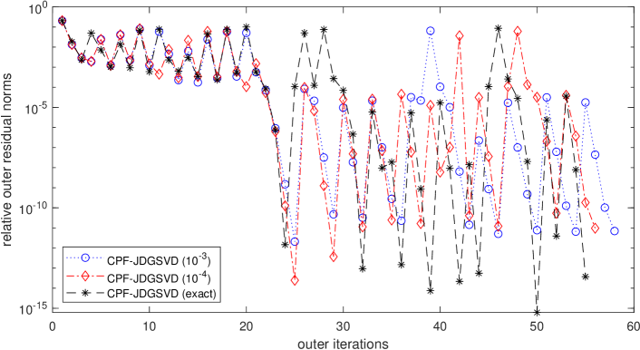
Fig. 1: Computing the GSVD components of $(A,B)=(\mathrm{deter4}^{T},B_{0})$ corresponding to the nine generalized singular values closest to $\tau=0.08$.

Tabel 3 reports the results, and Figure 1 depicts the convergence curves of CPF-JDGSVD with $\widetilde{\varepsilon}=10^{-3}$, $10^{-4}$ and the “exact” CPF-JDGSVD for computing nine GSVD components of $(A,B)$, where the GSVD components are computed one by one and the convergence curve, therefore, has nine stages for each $\widetilde{\varepsilon}$. We observe from Table 3 and Figure 1 that, regarding the outer iterations, for $\ell=1,5$ and $9$, CPF-JDGSVD with $\widetilde{\varepsilon}=10^{-3}$ and $10^{-4}$ behaves very much like its exact counterpart. Furthermore, we have found that, compared with the iterative exact CPF-JDGSVD, i.e., $\widetilde{\varepsilon}\!=\!10^{-15}$, the inexact CPF-JDGSVD algorithm costs only less than $53\%$ of total inner iterations or less than $61\%$ of total CPU time to compute the desired GSVD components. Clearly, a smaller $\widetilde{\varepsilon}$ is unnecessary since it cannot reduce outer iterations and instead increases the total cost substantially. Therefore, in the sequel, we adopt the default $\widetilde{\varepsilon}\!=\!10^{-3}$ in CPF-JDGSVD and JDGSVD.

Experiment 5.3.

We compute the GSVD components of some other problems in Table 1. We write the matrix pairs $(A_{a},B_{a})\!=\!(\mathrm{lp\_bnl2}^{T},B_{0})$, $(A_{b},B_{b})\!=\!(\mathrm{large}^{T},B_{0})$ and $(A_{c},B_{c})\!=\!(\mathrm{gemat1}^{T},B_{0})$ with the targets $\tau_{a}=20$, $\tau_{b}=5$ and $\tau_{c}=12$, respectively. The desired GSVD components are all clustered interior ones. We also test the large scale matrix pairs $(A_{d},B_{d})\!=\!(\mathrm{tmgpc1},B_{0})$, $(A_{e},B_{e})\!=\!(\mathrm{wstn\_1}^{T},B_{0})$ and $(A_{f},B_{f})\!=\!(\mathrm{degme}^{T},B_{0})$ with $\tau_{d}=2.7$, $\tau_{e}=7$ and $\tau_{f}=1.3$, respectively. The desired GSVD components correspond to the largest, interior and smallest ones of $(A_{d},B_{d})$, $(A_{e},B_{e})$ and $(A_{f},B_{f})$, respectively.

Table 4: Results of CPF-JDGSVD on some of the problems in Table 1.

$A$	$\ell=1$			$\ell=5$			$\ell=9$
	$I_{out}$	$I_{in}$	$T_{cpu}$	$I_{out}$	$I_{in}$	$T_{cpu}$	$I_{out}$	$I_{in}$	$T_{cpu}$
$\mathrm{lp\_bnl2}^{T}$	11	497	0.09	38	1841	0.28	68	​​3752​​	0.54
$\mathrm{large}^{T}$	7	​​9528​​	1.71	47	​​76190​​	13.7	61	​​132107​​	25.6
$\mathrm{gemat1}^{T}$	8	​​6900​​	1.90	23	​​22257​​	6.71	40	​​33336​​	10.7
$\mathrm{tmgpc1}$	8	403	1.82	27	1234	6.31	54	2752	15.0
$\mathrm{wstn\_1}^{T}$	13	​​​​35982  ​​​​	​​​​5.29e+2​​​​	32	​​​​106212  ​​​​	​​​​1.90e+3​​​​	51	​​​​167817  ​​​​	​​​​3.46e+3​​​​
$\mathrm{degme}^{T}$	​​8​​	92	5.16	​​112​​	1399	83.3	​​261​​	3347	​​2.01e+2​​

Table 5: Results of JDGSVD on some of the problems in Table 1.

$A$	$\ell=1$			$\ell=5$			$\ell=9$
	​​$I_{out}$​​	$I_{in}$	$T_{cpu}$	​​$I_{out}$​​	$I_{in}$	$T_{cpu}$	​​$I_{out}$​​	$I_{in}$	$T_{cpu}$	$Relres_{t}$
​​$\mathrm{lp\_bnl2}^{T}$​​	​​10​​	​​918​​	0.20	​​37​​	​​3023​​	0.78	​​64​​	​​5640​​	1.51	2.19e-10​​
​​$\mathrm{large}^{T}$​​	​​7​​	​​9786​​	2.80	​​26​​	​​71127​​	24.4	​​43​​	​​137692​​	49.7	2.08e-10
​​$\!\!\mathrm{gemat1}^{T}$​​	​​13​​	​​10846​​	5.59	​​31​​	​​24986​​	13.6	​​48​​	​​36553​​	20.4	1.75e-10​​
​​$\mathrm{tmgpc1}$​​	​​8​​	​​807​​	6.29	​​24​​	​​1987​​	17.2	​​42​​	​​4282​​	40.4	1.25e-9​​
​​$\mathrm{wstn\_1}^{T}$​​	​​10​​	​​​​51244​​​​	​​2.17e+3​​​​	​​23​​	​​​​131417​​​​	​6.40e+3​​	​​41​​	​​​​206423​​​​	​​1.11e+4​​​​	4.25e-10​​
​​$\mathrm{degme}^{T}$​​	​​10​​	​​582​​	​​40.4​​	​​​​353​​​​	​​​​20673​​​​	​1.75e+3​​	​​​​998​​​​	​​​​64200​​​​	​​​​6.79e+3​​​​	1.22e-9​​

For these six test problems, we have observed very similar phenomena to those for the previous two examples. Table 4 reports the results, where the results on $(A_{e},B_{e})$ are obtained by CPF-JDGSVD with the fixed correction equation (4.9) solved, since for this problem we have noticed that CFP-JDGSVD with $fixtol=10^{-4}$ used too many inner iterations but comparable outer iterations. Table 4 indicates that CPF-JDGSVD worked efficiently for computing both the interior and the extreme GSVD components of the test matrix pairs. Particularly, we have seen that the outer iterations for $\ell=5$ and $9$ are only slightly more than those for $\ell=1$, confirming the effectiveness of the restarting scheme proposed in Section 4.2, where the reduced $\widetilde{\mathcal{X}}_{\rm new}$’s of purging the converged right generalized singular vectors from the current subspaces indeed retain rich information on the next desired right generalized singular vectors.

For these six problems, all the $B$ are well conditioned with $\kappa(B)\approx 5$. We have also applied the JDGSVD algorithm [13] to these problems with all the parameters same as in the CPF-JDGSVD algorithm. Table 5 displays the results, where $Relres_{t}$ is the relative residual norm whose entries are the $\ell$ $relres_{t}$ of converged GSVD components defined by (5.3). We see from Table 5 that for all the six problems, the relative residual norms of the converged approximate GSVD components computed by JDGSVD are very comparable to the stopping tolerance $10^{-10}$, as is expected since matrices $B$ are very well conditioned. Comparing Table 4 with Table 5, we can see that CPF-JDGSVD uses very comparable outer iterations as JDGSVD for the first five matrix pairs but it is at least three times as fast as JDGSVD for the last problem with $\ell=5,9$. Regarding the overall efficiency, CPF-JDGSVD uses fewer inner iterations or less than $52\%$ of CPU time to compute the desired nine GSVD components of $(A_{b},B_{b})$, $(A_{c},B_{c})$ and $(A_{e},B_{e})$. It reduces more than $33\%$ of inner iterations and more than $63\%$ of CPU time to compute all the desired GSVD components of $(A_{a},B_{a})$ and $(A_{b},B_{b})$. For $(A_{f},B_{f})$, CPF-JDGSVD significantly outperforms JDGSVD by using $5\%$ of inner iterations and $3\%$ of CPU time to converge. Therefore, for the matrix pairs with the full column rank and well-conditioned $B$, CPF-JDGSVD is more efficient than or at least competitive with JDGSVD.

Experiment 5.4.

We use CPF-JDGSVD and JDGSVD to compute nine GSVD components of $(A,B)=(\mathrm{blckhole},B_{1}^{T})$ corresponding to the generalized singular values closest to $\tau=1000$, where $\mathrm{blckhole}$ is a $2132\times 2132$ sparse matrix from [8] and $B=B_{1}^{T}$ ensures that $B$ has full column rank. The desired generalized singular values are the largest ones of $(A,B)$ and are well separated from each other.

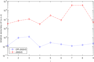
(a)

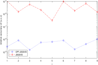
(b)

Fig. 2: (a) and (b) Accuracy of the converged generalized singular vectors of $(A,B)=(\mathrm{blckhole},B_{1}^{T})$ with $\tau=10^{3}$ and $(A,B)=(\mathrm{plddb}^{T},B_{2}^{T})$ with $\tau=70$ computed by CPF-JDGSVD and JDGSVD, respectively.

Table 6: Results on $A=\mathrm{blckhole}$ and $B=B_{1}^{T}$.

Matrix Pair	$\tau$	CPF-JDGSVD			JDGSVD
		$I_{out}$	$I_{in}$	$T_{cpu}$	$I_{out}$	$I_{in}$	$T_{cpu}$	$Relres_{t}$
$(A,B)$	$10^{+3}$	41	33671	2.07	658	347376	61.0	1.96e-8
$(B,A)$	$10^{-3}$	36	27441	1.67	2132	1583593	3.45e+2	1.33e-3

For this problem, both $A$ and $B$ are well conditioned with $\kappa(A)=4.17\times 10^{3}$, $\kappa(B)=1.36\times 10^{3}$ and $\kappa(\begin{bmatrix}\begin{smallmatrix}A\\ B\end{smallmatrix}\end{bmatrix})=26.6$. The largest and smallest generalized singular values of $(A,B)$ are $4.68\times 10^{3}$ and $1.21\times 10^{-3}$, respectively. Table 6 displays the results, and Figure 2a depicts the accuracy of the converged generalized singular vectors obtained by CPF-JDGSVD and JDGSVD, where the accuracy of a converged generalized singular vector triplet $(\tilde{u},\tilde{v},\tilde{x})$ is measured by

(5.4) $$\epsilon_{(\tilde{u},\tilde{v},\tilde{x})}=\sqrt{\sin^{2}\angle(\tilde{u},u)+\sin^{2}\angle(\tilde{v},v)+\sin^{2}\angle(\tilde{x},x)}$$

with the “exact” generalized singular vectors $(u,v,x)$ computed by gsvd.

We see from Table 6 that CPF-JDGSVD is much more efficient than JDGSVD, and it uses less than $10\%$ of outer and inner iterations and less than $4\%$ of CPU time than the latter. We have observed that all the generalized singular values computed by the two algorithms are accurate with the relative errors lying in $[10^{-15},10^{-11}]$. However, as can be seen from Figure 2, all the desired generalized singular vectors computed by CPF-JDGSVD are very accurate by recalling that we have used the stopping tolerance $tol=10^{-10}$, and they are two to nearly five orders more accurate than those computed by JDGSVD. Indeed, we see from Table 6 that the relative residual norms of the converged approximate GSVD components obtained by JDGSVD are a few orders larger than the stopping tolerance $10^{-10}$. This shows that transforming the GSVD problem into the generalized eigenvalue problems in [13] is not a general-purpose good choice since a backward stable algorithm for the generalized eigenvalue problems cannot produce backward stable approximate GSVD components of the original GSVD problem, especially when $\kappa(A)$ or $\kappa(B)$ is not small, as proved in [16]. In addition, we have observed that CPF-JDGSVD successively computed the desired GSVD components of $(A,B)$ one by one correctly while JDGSVD only succeeded to compute the first six desired GSVD components and then repeatedly computed the first one after the six ones had converged. This phenomenon occurs since $B^{T}B$ is quite ill conditioned with $\kappa(B^{T}B)=1.85\times 10^{6}$ and the right searching subspace involved in JDGSVD, which should be made $B^{T}B$-orthogonal to the converged right generalized singular vectors by solving some appropriate correction equations, loses $B^{T}B$-orthogonality to the converged right generalized singular subspace, so that the information on the converged GSVD component reappeared and caused repeated computation of the same GSVD component.

Since the GSVD of $(A,B)$ is equivalent to that of $(B,A)$, we have also applied CPF-JDGSVD and JDGSVD to $(B,A)$ with $\tau=10^{-3}$ to compute nine GSVD components of $(B,A)$. We have found that JDGSVD successfully computes the first eight desired GSVD components of $(B,A)$. However, the desired generalized singular values of $(A,B)$ corresponds to the smallest clustered ones of $(B,A)$. It may be this reason that made that JDGSVD fail to compute the ninth desired GSVD component when total $n$ outer iterations have been used and the relative residual norm of the computed approximate GSVD component could not drop below $10^{-4}$ after $2132$ outer iterations were exhausted. In contrast, as we see from Table 6, CPF-JDGSVD succeeds to compute all the desired GSVD components accurately and uses even fewer outer and inner iterations and less CPU time than it does when applied to $(A,B)$ with $\tau=10^{3}$.

Experiment 5.5.

We use CPF-JDGSVD and JDGSVD to compute the nine GSVD components of the matrix pair $(A,B)=(\mathrm{plddb}^{T},B_{2}^{T})$ corresponding to the generalized singular values closest to $\tau=70$, where $B_{2}$ is the $n\times(n+2)$ scaled discrete approximation of the second order derivation operator of dimension one:

$$B_{2}=\begin{bmatrix}-1&2&-1&&\\ &\ddots&\ddots&\ddots&\\ &&-1&2&-1\end{bmatrix}\in\mathbb{R}^{n\times(n+2)}.$$

The desired generalized singular values are the interior ones of $(A,B)$ and highly clustered with each other.

For this problem, $\kappa(A)=1.23\times 10^{4}$, $\kappa(B)=1.69\times 10^{6}$, and $\kappa(\begin{bmatrix}\begin{smallmatrix}A\\ B\end{smallmatrix}\end{bmatrix})=1.40\times 10^{2}$. Therefore, both $A$ and $B$ are not well conditioned, and it is expected that JDGSVD cannot compute generalized singular vectors accurately while CPF-JDGSVD works well. We observe that CPF-JDGSVD uses $96$ outer iterations and $119874$ inner iterations, about twice of $44$ outer and $67330$ inner iterations used by JDGSVD. All the generalized singular values computed by JDGSVD and CPF-JDGSVD are very accurate with the relative errors lying in $[10^{-15},10^{-13}]$. Unfortunately, as has been depicted in Figure 2b, we see that the generalized singular vectors computed by CPF-JDGSVD are very accurate and are a few orders more accurate than those computed by JDGSVD. We have also applied CPF-JDGSVD and JDGSVD to the matrix pair $(B,A)$ with $\tau=\frac{1}{70}$ and observed similar accuracy advantage of CPF-JDGSVD over JDGSVD.

Experiment 5.6.

We compute the GSVD components of the other problems in Table 1: $(A_{a},B_{a})\!=(\mathrm{slptsk}^{T},B_{1})$, $(A_{b},B_{b})\!=(\mathrm{rosen10}^{T},B_{1})$, $(A_{c},B_{c})\!=(\mathrm{flower54}^{T},B_{1})$, $(A_{d},B_{d})=(\mathrm{l30}^{T},B_{1})$, $(A_{e},B_{e})=(\mathrm{cq5}^{T},B_{1})$ and $(A_{f},B_{f})=(\mathrm{stat96v5}^{T},B_{1})$ with the targets $\tau$ being $\tau_{a}=9$, $\tau_{b}=4$, $\tau_{c}=82$, $\tau_{d}=1$, $\tau_{e}=0.1$ and $\tau_{f}=4000$, respectively.

Table 7: Results of applying CPF-JDGSVD to some of the problems in Table 1.

$A$	$\ell=1$			$\ell=5$			$\ell=9$
	$I_{out}$	$I_{in}$	$T_{cpu}$	$I_{out}$	$I_{in}$	$T_{cpu}$	$I_{out}$	$I_{in}$	$T_{cpu}$
$\mathrm{slptsk}^{T}$	7	6589	0.80	32	23551	3.04	67	41350	7.02
$\mathrm{rosen10}^{T}$	6	2003	0.25	23	7308	0.95	41	12373	1.87
$\mathrm{flower54}^{T}$	15	39636	14.5	37	96769	36.5	66	157342	61.2
$\mathrm{l30}^{T}$	6	47	0.03	83	2550	0.66	96	3641	0.95
$\mathrm{cq5}^{T}$	12	35583	10.2	22	54841	16.4	30	62921	19.2
$\mathrm{stat96v5}^{T}$	12	8350	2.94	28	16403	5.84	50	24991	9.69

Notice from (5.1) that the matrices $B$ in the matrix pairs are rank deficient with $\mathcal{N}(B)={\rm span}\{[1,\dots,1]^{T}\}$ and from Table 1 that $A_{f}=\mathrm{stat96v5}^{T}$ is also rank deficient. As shown in Table 7, for these problems, CPF-JDGSVD succeeds to compute all the desired GSVD components, i.e., the clustered interior ones of $(A_{i},B_{i})$, $i=a,b,c,d$, the clustered smallest ones of $(A_{e},B_{e})$ and the largest nontrivial ones of $(A_{f},B_{f})$.

Finally, we pay special attention to the inner iterations. The correction equation (4.8) or (4.9) is symmetric indefinite and may be ill conditioned, which is definitely true when the desired generalized singular values $\sigma$’s are interior ones or clustered. When MINRES is used to solve (4.8) or (4.9), preconditioning is naturally appealing. Unfortunately, it is generally hard to effectively precondition such correction equations. We have used the MATLAB built-in function ilu with $setup.droptol=0.1$ and $0.01$ to compute sparse incomplete LU factorizations of $A^{T}A-\theta^{2}B^{T}B$ and $A^{T}A-\tau^{2}B^{T}B$ as preconditioners, and solved the resulting preconditioned nonsymmetric correction equations using the BiCGStab algorithm [24]. We have found that such preconditioners are very often ineffective and, for many of the test problems, the preconditioned BiCGStab is inferior to the unpreconditioned MINRES and uses more inner iterations. Therefore, we do not present the results of using the preconditioned BiCGStab.

6 Conclusions

We have proposed a CPF-JDGSVD method for computing a partial GSVD of the large regular matrix pair $(A,B)$. In the outer iterations, the method is a standard Rayleigh–Ritz projection that implicitly solves the mathematically equivalent generalized eigenvalue problem of $(A^{T}A,B^{T}B)$ without explicitly forming the cross-product matrices, so that it avoids the possible accuracy loss of the computed GSVD components. In the inner iterations, the algorithm approximately solves the correction equations iteratively. We have established a convergence result on the approximate generalized singular values and analyzed the inner and outer iterations in some depth. Based on the results obtained, we have proposed reliable stopping criteria for the inner iterations. To be more practical, we have focused on several issues and have developed a thick-restart CPF-JDGSVD algorithm with deflation for computing more than one GSVD components of $(A,B)$ corresponding to the generalized singular values closest to $\tau$.

Numerical experiments have confirmed the efficiency, reliability and accuracy of the thick-restart CPF-JDGSVD algorithm with deflation for computing both some interior and extreme GSVD components of a large regular matrix pair. We have numerically compared CPF-JDGSVD with JDGSVD and justified the great superiority of the former to the latter when computing generalized singular vectors accurately.

References

- [1] Z. Bai, J. Demmel, J. Dongarra, A. Ruhe, and H. A. Van der Vorst, Templates for the Solution of Algebraic Eigenvalue Problems: A Practical Guide, SIAM, Philadelphia, PA, 2000.
- [2] T. Betcke, The generalized singular value decomposition and the method of particular solutions, SIAM J. Sci. Comput., 30 (2008), pp. 1278–1295.
- [3] Å. Björck, Numerical Methods for Least Squares Problems, SIAM, Philadelphia, PA, 1996.
- [4] K.-W. E. Chu, Singular value and generalized singular value decompositions and the solution of linear matrix equations, Linear Algebra Appl., 88 (1987), pp. 83–98.
- [5] K. Chui, Charles and J. Wang, Randomized anisotropic transform for nonlinear dimensionality reduction, Int. J. Geomath, 1 (2010), pp. 23–50.
- [6] R. R. Coifman and S. Lafon, Diffusion maps, Appl. Comput. Harmon. Anal., 21 (2006), pp. 5–30.
- [7] R. R. Coifman, S. Lafon, A. B. Lee, M. Maggioni, B. Nadler, F. Warner, and S. W. Zucker, Geometric diffusions as a tool for harmonic analysis and structure definition of data: Multiscale methods, PNAS, 21 (2006), pp. 5–30.
- [8] T. A. Davis and Y. Hu, The University of Florida sparse matrix collection, ACM Trans. Math. Software, 38 (2011), pp. 1–25. Data available online at \urlhttp://www.cise.ufl.edu/research/sparse/matrices/.
- [9] G. H. Golub and C. F. van Loan, Matrix Computations, 4th Ed., John Hopkins University Press, 2012.
- [10] A. Greenbaum, Iterative Methods for Solving Linear Systems, SIAM, Philadephia, PA, 1997.
- [11] P. C. Hansen, Regularization, GSVD and truncated GSVD, BIT, 29 (1989), pp. 491–504.
- [12] P. C. Hansen, Rank-Deficient and Discrete Ill-Posed Problems: Numerical Aspects of Linear Inversion, SIAM, Philadelphia, PA, 1998.
- [13] M. E. Hochstenbach, A Jacobi–Davidson type method for the generalized singular value problem, Linear Algebra Appl., 431 (2009), pp. 471–487.
- [14] P. Howland, M. Jeon, and H. Park, Structure preserving dimension reduction for clustered text data based on the generalized singular value decomposition, SIAM J. Matrix Anal. Appl., 25 (2003), pp. 165–179.
- [15] J. Huang and Z. Jia, On inner iterations of Jacobi-Davidson type methods for large SVD computations, SIAM J. Sci. Comput., 41 (2019), pp. A1574–A1603.
- [16] J. Huang and Z. Jia, On choices of formulations of computing the generalized singular value decomposition of a matrix pair, Numer. Algor., (2020). doi: 10.1007/s11075-020-00984-9.
- [17] Z. Jia and C. Li, Inner iterations in the shift–invert residual Arnoldi method and the Jacobi–Davidson method, Sci. China Math., 57 (2014), pp. 1733–1752.
- [18] Z. Jia and C. Li, Harmonic and refined harmonic shift-invert residual Arnoldi and Jacobi–Davidson methods for interior eigenvalue problems, J. Comput. Appl. Math., 282 (2015), pp. 83–97.
- [19] Z. Jia and G. Stewart, An analysis of the Rayleigh–Ritz method for approximating eigenspaces, Math. Comput., 70 (2001), pp. 637–647.
- [20] Z. Jia and Y. Yang, A joint bidiagonalization based iterative algorithm for large scale general-form tikhonov regularization, Appl. Numer. Math., 157 (2020), pp. 159–177.
- [21] B. Kågström, The generalized singular value decomposition and the general (AB)-problem, BIT, 24 (1984), pp. 568–583.
- [22] C. C. Paige and M. A. Saunders, Towards a generalized singular value decomposition, SIAM J. Numer. Anal., 18 (1981), pp. 398–405.
- [23] C. H. Park and H. Park, A relationship between linear discriminant analysis and the generalized minimum squared error solution, SIAM J. Matrix Anal. Appl., 27 (2005), pp. 474–492.
- [24] Y. Saad, Iterative Methods for Sparse Linear Systems, 2nd Ed., SIAM, Philadelphia, PA, 2003.
- [25] A. Stathopoulos, Y. Saad, and K. Wu, Dynamic thick restarting of the Davidson and the implicitly restarted Arnoldi methods, SIAM J. Sci. Comput., 19 (1998), pp. 227–245.
- [26] G. W. Stewart and J. G. Sun, Matrix Perturbation Theory, Acadmic Press, Inc., Boston, 1990.
- [27] S. Van Huffel and P. Lemmerling, Total Least Squares and Errors-in-Variables Modeling, Kluwer Academic Publishers, 2002.
- [28] C. F. van Loan, Generalizing the singular value decomposition, SIAM J. Numer. Anal., 13 (1976), pp. 76–83.
- [29] H. Zha, Computing the generalized singular values/vectors of large sparse or structured matrix pairs, Numer. Math., 72 (1996), pp. 391–417.
- [30] I. N. Zwaan, Cross product-free matrix pencils for computing generalized singular values, (2019). arXiv:1912.08518 [math.NA].
- [31] I. N. Zwaan and M. E. Hochstenbach, Generalized Davidson and multidirectional-type methods for the generalized singular value decomposition, (2017). arXiv:1705.06120 [math.NA].