Optimal designs for some bivariate cokriging models

Abstract

This article focuses on the estimation and design aspects of a bivariate collocated cokriging experiment. For a large class of covariance matrices, a linear dependency criterion is identified, which allows the best linear unbiased estimator of the primary variable in a bivariate collocated cokriging setup to reduce to a univariate kriging estimator. Exact optimal designs for efficient prediction for such simple and ordinary reduced cokriging models with one-dimensional inputs are determined. Designs are found by minimizing the maximum and the integrated prediction variance, where the primary variable is an Ornstein-Uhlenbeck process. For simple and ordinary cokriging models with known covariance parameters, the equispaced design is shown to be optimal for both criterion functions. The more realistic scenario of unknown covariance parameters is addressed by assuming prior distributions on the parameter vector, thus adopting a Bayesian approach to the design problem. The equispaced design is proved to be the Bayesian optimal design for both criteria. The work is motivated by designing an optimal water monitoring system for an Indian river.

Keywords: Cross-covariance, Equispaced designs, Exponential Covariance , Gaussian Processes, Mean squared error of prediction

1 Introduction

Kriging is a method for estimating a variable of interest, known as the primary variable, at unknown input sites. When multiple responses are collected, multivariate kriging, also known as cokriging, is a related method for estimating the variable of interest at a specific location using measurements of this variable at other input sites along with the measurements of auxiliary/secondary variables, which may provide useful information about the primary variable (Myers,, 1983, 1991; Wackernagel,, 2003; Chiles and Delfiner,, 2009). For example, consider a water quality study in which a geologist is interested in estimating pH levels (primary response) at several unsampled locations along a river, but auxiliary information such as phosphate concentration or amount of dissolved oxygen may facilitate more accurate estimates of pH levels. We may also consider a computer experiment, where the engineering code produces the primary response and its partial derivatives. The partial derivatives (secondary variables) provide valuable information about the response (Santner et al.,, 2010). This scenario is typical when the responses measured are correlated, both non-spatially (at the same input sites) and spatially (over different sites, particularly those close to each other).

Very little is known about designs for such cokriging models. Li and Zimmerman, (2015), Madani and Emery, (2019), Bueso et al., (1999), Le and Zidek, (1994), Caselton and Zidek, (1984) developed optimal designs for multivariate kriging models or multivariate spatial processes, however the designs were all based on numerical simulations. The key difficulty in using such multivariate models is specifying the cross-covariance between the different random processes. Unlike direct covariance matrices, cross-covariance matrices need not be symmetric; indeed, these matrices must be chosen in such a way that the second-order structure always yields a non-negative definite covariance matrix (Genton and Kleiber,, 2015; Subramanyam and Pandalai,, 2004). A broad list of valid covariance structures for multivariate kriging models has been proposed by Li and Zimmerman, (2015).

In this article, we address two issues for bivariate cokriging experiments, (i) estimation of the primary variable and (ii) determining optimal designs by minimizing the mean squared error of the estimation. In the first couple of sections, we discuss simple and ordinary bivariate collocated cokriging models, the various covariance functions available in the literature for such models, and their estimation aspects. Specifically, we consider two stationary and isotropic random functions, $Z_{1}$ and $Z_{2}$ over $\mathcal{D}\subseteq\mathbb{R}$, where $Z_{1}$ is the primary variable and $Z_{2}$ is the secondary/auxiliary variable. Our main interest is in the prediction of $Z_{1}$, at a single location, say $x_{0}$, in the region of interest. For defining covariance matrices for the bivariate responses, we mainly utilize two families of stationary covariances, namely the generalized Markov-type and the proportional covariance functions. The generalized Markov-type covariance, an extended version of Markov-type covariance, is a new function proposed in this article. Along with the generalized Markov-type and proportional covariances, the other covariance types mentioned by Li and Zimmerman, (2015) are also studied. We prove a linear dependency condition under which the best linear unbiased predictor (BLUP) of $Z_{1}(x_{0})$ in a bivariate cokriging model is shown to be equivalent to the BLUP in a univariate kriging setup. A wide class of covariance functions is identified which allows this reduction.

In the later part of the article, we determine optimal designs for some cokriging models, particularly those for which the reduction holds true. We consider the maximum and the integrated cokriging variance of $Z_{1}(x_{0})$ as the two design criterion functions. The primary variable is assumed to have an isotropic exponential covariance, that is, it satisfies $Cov[Z_{1}(x),Z_{1}(x^{\prime})]=\sigma_{11}\;{e}^{-\theta|x-x^{\prime}|}$ with marginal variance $\sigma_{11}>0$ and the exponential parameter $\theta>0$. Note, $Z_{1}(x_{0})$ is also called an Ornstein–Uhlenbeck process (Antognini and Zagoraiou,, 2010). For known covariance parameters in simple and ordinary cokriging models, we prove that the equispaced design minimizes the maximum and integrated prediction variance, that is, it is both G-optimal and I-optimal. In real life, however, covariance parameters are most likely unknown. To address the dependency of the design selection criterion on the unknown covariance parameters, we assume prior distributions on the parameter vector and instead determine pseudo-Bayesian optimal designs. The equispaced design is also proved to be the Bayesian I- and G-optimal design.

The original contributions of this article include (i) a linear dependency condition for reduction of collocated bivariate kriging estimators to a kriging estimator, (ii) the generalized Markov-type covariance, (iii) G-optimal designs for known covariance parameters and G-optimal Bayesian designs, for such simple and ordinary reduced bivariate cokriging models and (iv) I-optimal Bayesian designs.

We stress that our sole objective is to find theoretical, exact optimal designs, not numerical designs, for bivariate cokriging models. For this reason, we consider only the exponential covariance structure for the primary variable $Z_{1}$. Note no theoretical exact optimal designs for covariance structures other than the exponential covariance are currently available in the statistical literature.

Many researchers have studied D- and I-optimal designs for univariate kriging experiments with an exponential covariance structure. For single responses and one-dimensional inputs, Kisel’ák and Stehlík, (2008), Zagoraiou and Antognini, (2009), Antognini and Zagoraiou, (2010) proved that equispaced designs are optimal for trend parameter estimation with respect to average prediction error minimization and the D-optimality criterion. For the information gain (entropy criterion) also, the equispaced design was proved to be optimal by Antognini and Zagoraiou, (2010). Zimmerman, (2006) studied designs for universal kriging models and showed how the optimal design differs depending on whether covariance parameters are known or estimated using numerical simulations on a two-dimensional grid. Diggle and Lophaven, (2006) proposed Bayesian geostatistical designs focusing on efficient spatial prediction while allowing the parameters to be unknown. Exact optimal designs for linear and quadratic regression models with one-dimensional inputs and error structure of the autoregressive of order one form were determined by Dette et al., (2008). This work was further extended by Dette et al., (2013) to a broader class of covariance kernels, where they also showed that the arcsine distribution is universally optimal for the polynomial regression model with correlation structure defined by the logarithmic potential. Baran et al., (2013) and Baran and Stehlík, (2015) investigated optimal designs for parameters of shifted Ornstein-Uhlenbeck sheets for two input variables. More recently, Sikolya and Baran, (2020) worked with the prediction of a complex Ornstein-Uhlenbeck process and derived the optimal design with respect to the entropy maximization criterion.

In Sections 2 and 3 we introduce bivariate cokriging models and the related functions, respectively. The linear dependency condition which allows the BLUP of a cokriging model to reduce to the BLUP of a kriging model is discussed in Section 4. In Section 5, we discuss optimal designs for some cokriging models with known and unknown parameters. An illustration using a water quality data set is provided in Section 6. Concluding remarks are given in Section 7.

2 Cokriging models and their estimation

In this section, multivariate kriging models along with their direct covariance and cross-covariance structures are defined. Our focus is on bivariate processes with one-dimensional inputs. Consider two simultaneous random functions $Z_{1}(\cdot)$ and $Z_{2}(\cdot)$, where $Z_{1}(\cdot)$ is the primary response and $Z_{2}(\cdot)$ the secondary response.

We assume both responses are observed over the region $\mathcal{D}\subseteq\mathbb{R}$. In multivariate studies, usually the sets of points at which different random functions are observed might not coincide, but in the case that it does, the design is said to be completely collocated or simply collocated (Li and Zimmerman,, 2015). In this article, we work with a completely collocated design and consider that $Z_{1}(\cdot)$ and $Z_{2}(\cdot)$ are both sampled at the same set of points $\mathcal{S}=\{x_{1},x_{2},\ldots,x_{n}\}$, where $\mathcal{S}\subseteq\mathcal{D}\subseteq\mathbb{R}$. We consider $\mathbf{Z}_{i}$ to be the $n\times 1$ vector of all observations for the random function $Z_{i}(\cdot)$ for $i=1,2$. These random functions are characterized by their mean and covariance structures, with $E[Z_{i}(x)]=m_{i}(x)$ and $Cov(Z_{i}(x),Z_{j}(x^{\prime}))=\mathcal{C}_{ij}(x,x^{\prime}),\text{ for }x,x^{\prime}\in\mathcal{D}\text{ and }i,j=1,2$. The underlying linear model is given by:

$$\begin{pmatrix}\mathbf{Z}_{1}\\ \mathbf{Z}_{2}\end{pmatrix} =\begin{pmatrix}\boldsymbol{F}_{1}&\boldsymbol{0}\\ \boldsymbol{0}&\boldsymbol{F}_{2}\end{pmatrix}\begin{pmatrix}\boldsymbol{\pi}_{1}\\ \boldsymbol{\pi}_{2}\end{pmatrix}+\begin{pmatrix}\boldsymbol{\epsilon}_{1}\\ \boldsymbol{\epsilon}_{2}\end{pmatrix},$$ (1)

where $\boldsymbol{F}_{i}$ is the $n\times p_{i}$ matrix, with its $k^{th}$ row given by $\boldsymbol{f}_{i}^{T}(x_{k})$, $\boldsymbol{f}_{i}(x)$ is the $p_{i}\times 1$ vector of known basis drift functions $f_{i}^{l}(.)$ for $l=0,\ldots,p_{i}$ and $\boldsymbol{\pi}_{i}$ is the $p_{i}\times 1$ vector of parameters. From equation (1) we see $m_{i}(x)=\boldsymbol{f}_{i}^{T}(x)\boldsymbol{\pi}_{i}$ for $i=1,2\text{ and }x\in\mathcal{D}$. We assume $\boldsymbol{\epsilon}_{i}$ to be a zero mean column vector of length $n$ corresponding to the random variation of $\mathbf{Z}_{i}$. The error covariance is $Cov(\epsilon_{i}(x),\epsilon_{j}(x^{\prime}))=Cov(Z_{i}(x),Z_{j}(x^{\prime}))=\mathcal{C}_{ij}(x,x^{\prime}),\text{ for }x,x^{\prime}\in\mathcal{D}\text{ and }i,j=1,2$. Using matrix notation, the model in equation (1) can be rewritten as:

$$\mathbf{Z}=\boldsymbol{F}\boldsymbol{\pi}+\boldsymbol{\epsilon},$$ (2)

where $\mathbf{Z}=(\mathbf{Z}_{1}^{T},\mathbf{Z}_{2}^{T})^{T}$ is a $2n\times 1$ vector, $\boldsymbol{\epsilon}=(\boldsymbol{\epsilon}_{1}^{T},\boldsymbol{\epsilon}_{2}^{T})^{T}$, $\boldsymbol{\pi}=(\boldsymbol{\pi}_{1}^{T},\boldsymbol{\pi}_{2}^{T})^{T}$, and $\boldsymbol{F}=\begin{pmatrix}\boldsymbol{F}_{1}&\boldsymbol{0}\\ \boldsymbol{0}&\boldsymbol{F}_{2}\end{pmatrix}$. We are interested in predicting the value of the primary random function $Z_{1}(\cdot)$ at $x_{0}\in\mathcal{D}$, using the best linear unbiased predictor (BLUP). The true value of $Z_{1}(x_{0})$ is denoted by $Z_{0}$, that is, $Z_{1}(x_{0})\equiv Z_{0}$. A cokriging estimator of $Z_{0}$, as given by Chiles and Delfiner, (2009, Chapter 5), is an affine function of all available information on $Z_{1}(\cdot)$ and $Z_{2}(\cdot)$ at the $n$ sample points, given by $\displaystyle{\sum_{i=1,2}\boldsymbol{\lambda}_{i}^{T}\mathbf{Z}_{i}=\sum_{i=1,2}\sum_{j=1}^{n}\lambda_{ij}Z_{i}(x_{j}),}$ where $\boldsymbol{\lambda}_{i}=(\lambda_{i1},\lambda_{i2},\ldots,\lambda_{in})^{T}$ is an $n\times 1$ vector of weights for $i=1,2$. The cokriging estimators can be shown to be the BLUP of $Z_{0}$ (see Ver Hoef and Cressie,, 1993, for more details).

Some notations we use throughout the paper are: $\boldsymbol{\sigma}_{i0}=Cov(\mathbf{Z}_{i},Z_{0})$ for $i=1,2$, $\boldsymbol{\sigma}_{0}=(\boldsymbol{\sigma}_{10}^{T},\boldsymbol{\sigma}_{20}^{T})^{T}$ and $\sigma_{00}=Cov(Z_{0},Z_{0})$. The covariance matrices are denoted $Cov(\mathbf{Z}_{i},\mathbf{Z}_{j})=\boldsymbol{C}_{ij}$ for $i,j=1,2$, and the covariance of the entire vector $\mathbf{Z}$ is denoted $\boldsymbol{\Sigma}=\begin{bmatrix}\boldsymbol{C}_{11}&\boldsymbol{C}_{12}\\ \boldsymbol{C}_{21}&\boldsymbol{C}_{22}\\ \end{bmatrix}$. Note, $\boldsymbol{\Sigma}$ is a $2n\times 2n$ matrix.

2.1 Estimation in simple cokriging models

In a simple cokriging model, the means $m_{i}(x)$ are taken to be constant and known. Thus, without loss of generality, we may assume in such cases that the $Z_{i}$’s are zero mean processes for $i=1,2$ and therefore in this case $\boldsymbol{\pi}=(0,0)^{T}$. For known covariance parameters (Chiles and Delfiner,, 2009, Chapter 5) the cokriging estimator of $Z_{0}$, denoted by $Z^{\ast\ast}_{sck}$, and the cokriging variance, denoted by $\sigma^{2}_{sck}(x_{0})$, which is also the mean squared prediction error ($MSPE$) at $x_{0}$, are given by:

$$Z^{\ast\ast}_{sck} =\boldsymbol{\sigma}_{0}^{T}\boldsymbol{\Sigma}^{-1}\mathbf{Z},$$ (3)

$$\sigma^{2}_{sck}(x_{0}) =\sigma_{00}-\boldsymbol{\sigma}_{0}^{T}\boldsymbol{\Sigma}^{-1}\boldsymbol{\sigma}_{0}.$$ (4)

2.2 Estimation in ordinary cokriging models

Another popular model known as ordinary cokriging arises when the means are assumed to be constant but unknown, that is, $m_{i}(x)=\mu_{i},i=1,2$. In this case $\boldsymbol{\pi}=(\mu_{1},\mu_{2})^{T}$ and the basis drift functions are given by $f_{i}^{0}(x)=1$ for $i=1,2$. Hence, $\boldsymbol{F}=\begin{bmatrix}\boldsymbol{1}_{n}&\boldsymbol{0}_{n}\\ \boldsymbol{0}_{n}&\boldsymbol{1}_{n}\end{bmatrix},$ where $\boldsymbol{1}_{n}=(1,1,\ldots,1)_{n\times 1}^{T}$, and $\boldsymbol{0}_{n}=(0,0,\ldots,0)_{n\times 1}^{T}$. For known covariance parameters (Ver Hoef and Cressie,, 1993; Chiles and Delfiner,, 2009, Chapter 5) the ordinary cokriging estimator of $Z_{0}$, denoted by $Z^{\ast\ast}_{ock}$ and the cokriging variance, denoted by $\sigma^{2}_{ock}(x_{0})$, which is also the mean squared prediction error ($MSPE$) at $x_{0}$, are given by:

$$Z^{\ast\ast}_{ock} =\boldsymbol{\sigma}_{0}^{T}\boldsymbol{\Sigma}^{-1}\mathbf{Z}+(\boldsymbol{f}_{0}^{T}-\boldsymbol{\sigma}_{0}^{T}\boldsymbol{\Sigma}^{-1}\boldsymbol{F})(\boldsymbol{F}^{T}\boldsymbol{\Sigma}^{-1}\boldsymbol{F})^{-1}\boldsymbol{F}^{T}\boldsymbol{\Sigma}^{-1}\mathbf{Z},$$ (5)

$$\sigma^{2}_{ock}(x_{0}) =\sigma_{00}-\boldsymbol{\sigma}_{0}^{T}\boldsymbol{\Sigma}^{-1}\boldsymbol{\sigma}_{0}+(\boldsymbol{f}_{0}-\boldsymbol{F}^{T}\boldsymbol{\Sigma}^{-1}\boldsymbol{\sigma}_{0})^{T}(\boldsymbol{F}^{T}\boldsymbol{\Sigma}^{-1}\boldsymbol{F})^{-1}(\boldsymbol{f}_{0}-\boldsymbol{F}^{T}\boldsymbol{\Sigma}^{-1}\boldsymbol{\sigma}_{0}),$$ (6)

where $\boldsymbol{f}_{0}=(1,\;0)^{T}$.

3 Bivariate covariance functions

In Section 2, we noted the dependency of the cokriging estimators and their variances on the covariance functions. In this article, we consider only isotropic covariance functions, that is, $\mathcal{C}_{ij}(x,x^{\prime})$ is taken as $\mathcal{C}_{ij}(\left\lVert x-x^{\prime}\right\rVert)$ for $x,x^{\prime}\in\mathcal{D}$, where $\left\lVert\cdot\right\rVert$ is some norm function over $\mathcal{D}$.

We focus on two families of bivariate covariance functions, namely, i) the generalized Markov-type covariance and ii) the proportional covariance (see Journel, (1999), Chiles and Delfiner, (2009, Chapter 5), Banerjee et al., (2014, Chapter 9)). Note, that both of these families allow the primary variable to assume any valid covariance. Therefore we can generate a large number of covariance functions from these two families. Also, we will see that the most popularly used covariances belong to either one of these families. Optimal designs based on some of these covariance functions are discussed later.

The first family of bivariate covariance functions that we discuss is, the newly proposed generalized Markov-type covariance function. This is an extended form of the Markov-type covariance function mentioned in Chiles and Delfiner, (2009, Chapter 5) and Journel, (1999). Suppose the two random functions $Z_{1}(\cdot)$ and $Z_{2}(\cdot)$ have respective variances $\sigma_{11}$ and $\sigma_{22}$, where $\sigma_{11},\sigma_{22}>0$ and correlation coefficient $\rho$, $|\rho|<1$. If $(\sigma_{22}-\rho^{2}\sigma_{11})>0$, then the generalized Markov-type function is given as follows: the cross-covariance function $\mathcal{C}_{12}(\cdot)$ is considered to be proportional to $\mathcal{C}_{11}(\cdot)$ that is, $\mathcal{C}_{12}(h)=\rho\mathcal{C}_{11}(h)$, and the direct covariance for the secondary variable is given by $\mathcal{C}_{22}(h)=\rho^{2}\mathcal{C}_{11}(h)+(\sigma_{22}-\rho^{2}\sigma_{11})\mathcal{C}_{R}(h)$ for some valid correlogram $\mathcal{C}_{R}(.)$ and for $h\in\mathbb{R}$. Thus, the covariance matrix for the bivariate vector $\mathbf{Z}$ under the generalized Markov-type structure has the form:

$$\boldsymbol{\Sigma} =\begin{bmatrix}\boldsymbol{C}_{11}&\rho\boldsymbol{C}_{11}\\ \rho\boldsymbol{C}_{11}&\rho^{2}\boldsymbol{C}_{11}+(\sigma_{22}-\rho^{2}\sigma_{11})\boldsymbol{C}_{R}\end{bmatrix},$$ (7)

where $(\boldsymbol{C}_{11})_{ij}=\mathcal{C}_{11}(|x_{i}-x_{j}|)$ and $(\boldsymbol{C}_{R})_{ij}=\mathcal{C}_{R}(|x_{i}-x_{j}|)$ for $i,j=1,\ldots,n$. The validity of the proposed generalized Markov-type covariance function is discussed in details in A.1.

In the case of proportional covariances function, the direct covariance and cross-covariance of the random functions $Z_{1}(\cdot)$ and $Z_{2}(\cdot)$ are proportional to a single underlying covariance function, say $\mathcal{C}_{Q}(\cdot)$, that is, $\mathcal{C}_{ij}(h)=\sigma_{ij}\mathcal{C}_{Q}(h)$ for $i,j=1,2$ (see Chiles and Delfiner, (2009, Chapter 5), Banerjee et al., (2014, Chapter 9)). If, $\begin{bmatrix}\sigma_{11}&\sigma_{12}\\ \sigma_{21}&\sigma_{22}\end{bmatrix}$ is a positive definite matrix, Chiles and Delfiner, (2009) states that $\mathcal{C}_{ij}(\cdot)$ is a valid covariance function and hence $\boldsymbol{\Sigma}$ is a valid covariance matrix. Thus, under the proportional covariance model,

$$\boldsymbol{\Sigma}=\begin{bmatrix}\sigma_{11}\boldsymbol{Q}&\sigma_{12}\boldsymbol{Q}\\ \sigma_{21}\boldsymbol{Q}&\sigma_{22}\boldsymbol{Q}\end{bmatrix},\text{ where }(\boldsymbol{Q})_{ij}=\mathcal{C}_{Q}(|x_{i}-x_{j}|).$$ (8)

Some of the covariance functions, popularly used for bivariate cokriging models are Mat(0.5), Mat(1.5), Mat($\infty$), NS1, NS2, NS3 (listed in Table 1) (Li and Zimmerman, (2015)). Note that in fact Mat(0.5), Mat(1.5) and Mat($\infty$) belong to the proportional covariance family while covariance function NS1 belongs to the generalized Markov-type covariance family. Details are given in Table 1.

		Bivariate covariance function	Specifications
A.		Generalized Markov-Type	$\mathcal{C}_{11}(0)=\sigma_{11}$
		$|\rho|<1$	$\mathcal{C}_{22}(\left\lVert x-x^{\prime}\right\rVert)=\rho^{2}\mathcal{C}_{11}(\left\lVert x-x^{\prime}\right\rVert)+(\sigma_{22}-\rho^{2}\sigma_{11})\mathcal{C}_{R}(\left\lVert x-x^{\prime}\right\rVert)$
		$(\sigma_{22}-\rho^{2}\sigma_{11})>0$	$\mathcal{C}_{21}(\left\lVert x-x^{\prime}\right\rVert)=\rho\mathcal{C}_{11}(\left\lVert x-x^{\prime}\right\rVert)$
		$\sigma_{11},\sigma_{22}>0$	$\mathcal{C}_{12}(\left\lVert x-x^{\prime}\right\rVert)=\mathcal{C}_{21}(\left\lVert x-x^{\prime}\right\rVert)$
	a.	NS1	$\mathcal{C}_{11}(\left\lVert x-x^{\prime}\right\rVert)=\sigma_{11}\lambda^{\left\lVert x-x^{\prime}\right\rVert}$
			$\mathcal{C}_{22}(\left\lVert x-x^{\prime}\right\rVert)=\sigma_{22}\lambda_{c}^{2}\lambda^{\left\lVert x-x^{\prime}\right\rVert}+\sigma_{22}(1-\lambda_{c}^{2})\lambda^{2\left\lVert x-x^{\prime}\right\rVert}$
			$\mathcal{C}_{12}(\left\lVert x-x^{\prime}\right\rVert)=(\sigma_{11}\sigma_{22})^{1/2}\lambda_{c}\lambda^{\left\lVert x-x^{\prime}\right\rVert}$
			$\mathcal{C}_{12}(\left\lVert x-x^{\prime}\right\rVert)=\mathcal{C}_{21}(\left\lVert x-x^{\prime}\right\rVert)$
	(Taking, $\mathcal{C}_{11}(\left\lVert x-x^{\prime}\right\rVert)=\sigma_{11}\lambda^{\left\lVert x-x^{\prime}\right\rVert}$, $\rho=(\sigma_{11}/\sigma_{22})^{1/2}\lambda_{c}$, and $\mathcal{C}_{R}(\left\lVert x-x^{\prime}\right\rVert)=\lambda^{2\left\lVert x-x^{\prime}\right\rVert}$ in A.)
B.		Proportional Covariance	$\mathcal{C}_{11}(\left\lVert x-x^{\prime}\right\rVert)=\sigma_{11}\mathcal{C}_{Q}(\left\lVert x-x^{\prime}\right\rVert)$
		$(\sigma)_{ij}$ is a positive definite matrix	$\mathcal{C}_{22}(\left\lVert x-x^{\prime}\right\rVert)=\sigma_{22}\mathcal{C}_{Q}(\left\lVert x-x^{\prime}\right\rVert)$
		$\mathcal{C}_{Q}(\cdot)$ is any valid covariance function	$\mathcal{C}_{12}(\left\lVert x-x^{\prime}\right\rVert)=\sigma_{12}\mathcal{C}_{Q}(\left\lVert x-x^{\prime}\right\rVert)$
			$\mathcal{C}_{21}(\left\lVert x-x^{\prime}\right\rVert)=\sigma_{21}\mathcal{C}_{Q}(\left\lVert x-x^{\prime}\right\rVert)$
	b.	Mat(0.5)	$\mathcal{C}_{11}(\left\lVert x-x^{\prime}\right\rVert)=\sigma_{11}\lambda^{\left\lVert x-x^{\prime}\right\rVert}$
			$\mathcal{C}_{22}(\left\lVert x-x^{\prime}\right\rVert)=\sigma_{22}\lambda^{\left\lVert x-x^{\prime}\right\rVert}$
			$\mathcal{C}_{12}(\left\lVert x-x^{\prime}\right\rVert)=(\sigma_{11}\sigma_{22})^{1/2}\lambda_{c}\lambda^{\left\lVert x-x^{\prime}\right\rVert}$
			$\mathcal{C}_{12}(\left\lVert x-x^{\prime}\right\rVert)=\mathcal{C}_{21}(\left\lVert x-x^{\prime}\right\rVert)$
	(Taking, $\mathcal{C}_{Q}(\left\lVert x-x^{\prime}\right\rVert)=\lambda^{\left\lVert x-x^{\prime}\right\rVert}$ and $\sigma_{12}=(\sigma_{11}\sigma_{22})^{1/2}\lambda_{c}$ in B.)
	c.	Mat(1.5)	$\mathcal{C}_{11}(\left\lVert x-x^{\prime}\right\rVert)=\sigma_{11}[1-\left\lVert x-x^{\prime}\right\rVert log(\lambda)]\lambda^{\left\lVert x-x^{\prime}\right\rVert}$
			$\mathcal{C}_{22}(\left\lVert x-x^{\prime}\right\rVert)=\sigma_{22}[1-\left\lVert x-x^{\prime}\right\rVert log(\lambda)]\lambda^{\left\lVert x-x^{\prime}\right\rVert}$
			$\mathcal{C}_{12}(\left\lVert x-x^{\prime}\right\rVert)=(\sigma_{11}\sigma_{22})^{1/2}\lambda_{c}[1-\left\lVert x-x^{\prime}\right\rVert log(\lambda)]\lambda^{\left\lVert x-x^{\prime}\right\rVert}$
			$\mathcal{C}_{12}(\left\lVert x-x^{\prime}\right\rVert)=\mathcal{C}_{21}(\left\lVert x-x^{\prime}\right\rVert)$
	(Taking, $\mathcal{C}_{Q}(\left\lVert x-x^{\prime}\right\rVert)=[1-\left\lVert x-x^{\prime}\right\rVert log(\lambda)]\lambda^{\left\lVert x-x^{\prime}\right\rVert}$ and $\sigma_{12}=(\sigma_{11}\sigma_{22})^{1/2}\lambda_{c}$ in B.)
	d.	Mat($\infty$)	$\mathcal{C}_{11}(\left\lVert x-x^{\prime}\right\rVert)=\sigma_{11}\lambda^{\left\lVert x-x^{\prime}\right\rVert^{2}}$
			$\mathcal{C}_{22}(\left\lVert x-x^{\prime}\right\rVert)=\sigma_{22}\lambda^{\left\lVert x-x^{\prime}\right\rVert^{2}}$
			$\mathcal{C}_{12}(\left\lVert x-x^{\prime}\right\rVert)=(\sigma_{11}\sigma_{22})^{1/2}\lambda_{c}\lambda^{\left\lVert x-x^{\prime}\right\rVert^{2}}$
			$\mathcal{C}_{12}(\left\lVert x-x^{\prime}\right\rVert)=\mathcal{C}_{21}(\left\lVert x-x^{\prime}\right\rVert)$
	(Taking, $\mathcal{C}_{Q}(\left\lVert x-x^{\prime}\right\rVert)=\lambda^{\left\lVert x-x^{\prime}\right\rVert^{2}}$ and $\sigma_{12}=(\sigma_{11}\sigma_{22})^{1/2}\lambda_{c}$ in B.)
C.		NS2	$\mathcal{C}_{11}(\left\lVert x-x^{\prime}\right\rVert)=\sigma_{11}\lambda^{\left\lVert x-x^{\prime}\right\rVert}$
			$\mathcal{C}_{22}(\left\lVert x-x^{\prime}\right\rVert)=\sigma_{22}\lambda^{\left\lVert x-x^{\prime}\right\rVert}$
			$\mathcal{C}_{12}(\left\lVert x-x^{\prime}\right\rVert)=(\sigma_{11}\sigma_{22})^{1/2}\lambda_{c}\lambda^{\alpha\left\lVert x-x^{\prime}\right\rVert}$
			$\mathcal{C}_{12}(\left\lVert x-x^{\prime}\right\rVert)=\mathcal{C}_{21}(\left\lVert x-x^{\prime}\right\rVert)$
			where $\alpha=0.5,0.75,0.9$ according to whether $\lambda_{c}=0.2,0.5,0.8$
D.		NS3	$\mathcal{C}_{11}(\left\lVert x-x^{\prime}\right\rVert)=\sigma_{11}\lambda^{\left\lVert x-x^{\prime}\right\rVert}$
			$\mathcal{C}_{22}(\left\lVert x-x^{\prime}\right\rVert)=\sigma_{22}[1-\left\lVert x-x^{\prime}\right\rVert log(\lambda)+\left\lVert x-x^{\prime}\right\rVert^{2}(log(\lambda))^{2}/3]\lambda^{\left\lVert x-x^{\prime}\right\rVert}$
			$\mathcal{C}_{12}(\left\lVert x-x^{\prime}\right\rVert)=(\sigma_{11}\sigma_{22})^{1/2}\lambda_{c}[1-\left\lVert x-x^{\prime}\right\rVert log(\lambda)]\lambda^{\left\lVert x-x^{\prime}\right\rVert}$
			$\mathcal{C}_{12}(\left\lVert x-x^{\prime}\right\rVert)=\mathcal{C}_{21}(\left\lVert x-x^{\prime}\right\rVert)$

Table 1: Various bivariate covariance functions. Note, that $0<\lambda<1$, $|\lambda_{c}|<1$ and $\sigma_{11},\sigma_{22}>0$ .

4 Reduction of cokriging estimators to kriging

In this section, we discuss conditions under which the cokriging BLUP for the primary variable is reduced to a kriging BLUP. From Sections 2.1 and 2.2, it is not apparent that the cokriging and kriging estimators may be similar, particularly given the potentially non-zero correlation suggesting dependency between $Z_{1}(\cdot)$ and $Z_{2}(\cdot)$. However, in Lemma 4.1, we show that a linear dependency condition allows this reduction. Some covariance functions for which the reduction does not hold are also discussed.

We know that kriging is the univariate version of cokriging. Denoting the simple and ordinary kriging estimator of $Z_{0}$ by $Z^{\ast}_{sk}$ and $Z^{\ast}_{ok}$, respectively, and the respective variances ($MSPE$) at $x_{0}$ by $\sigma^{2}_{sk}(x_{0})$ and $\sigma^{2}_{ok}(x_{0})$, from Chiles and Delfiner, (2009) we have,

$$Z^{\ast}_{sk} =\boldsymbol{\sigma}_{10}^{T}\boldsymbol{C}_{11}^{-1}\mathbf{Z}_{1},$$ (9)

$$\sigma^{2}_{sk}(x_{0}) =\sigma_{00}-\boldsymbol{\sigma}_{10}^{T}\boldsymbol{C}_{11}^{-1}\boldsymbol{\sigma}_{10},$$ (10)

$$Z^{\ast}_{ok} =\boldsymbol{\sigma}_{10}^{T}\boldsymbol{C}_{11}^{-1}\mathbf{Z}_{1}+\dfrac{(1-\boldsymbol{\sigma}_{10}^{T}\boldsymbol{C}_{11}^{-1}\boldsymbol{1}_{n})(\boldsymbol{1}_{n}^{T}\boldsymbol{C}_{11}^{-1}\mathbf{Z}_{1})}{\boldsymbol{1}_{n}^{T}\boldsymbol{C}_{11}^{-1}\boldsymbol{1}_{n}},$$ (11)

$$\sigma^{2}_{ok}(x_{0}) =\sigma_{00}-\boldsymbol{\sigma}_{10}^{T}\boldsymbol{C}_{11}^{-1}\boldsymbol{\sigma}_{10}+\dfrac{(1-\boldsymbol{\sigma}_{10}^{T}\boldsymbol{C}_{11}^{-1}\boldsymbol{1}_{n})^{2}}{\boldsymbol{1}_{n}^{T}\boldsymbol{C}_{11}^{-1}\boldsymbol{1}_{n}}.$$ (12)

Lemma 4.1.

For a collocated bivariate cokriging problem with isotropic covariance structures, if the covariance functions $\mathcal{C}_{11}(.)$ and $\mathcal{C}_{12}(.)$ are linearly dependent; $Z^{\ast\ast}_{sck}$ (3) is equal to $Z^{\ast}_{sk}$ (9) and $Z^{\ast\ast}_{ock}$ (5) is equal to $Z^{\ast}_{ok}$ (11). Consequently, $\sigma^{2}_{sck}(x_{0})$ (4) and $\sigma^{2}_{ock}(x_{0})$ (6) are equal to $\sigma^{2}_{sk}(x_{0})$ (10) and $\sigma^{2}_{ok}(x_{0})$ (12), respectively.

Proof.

Consider $\boldsymbol{\Sigma}^{-1}$, which can be written as:

$$\boldsymbol{\Sigma}^{-1} =\begin{bmatrix}\boldsymbol{C}_{11}^{-1}+\boldsymbol{C}_{11}^{-1}\boldsymbol{C}_{12}(\boldsymbol{C}_{22}-\boldsymbol{C}_{21}\boldsymbol{C}_{11}^{-1}\boldsymbol{C}_{12})^{-1}\boldsymbol{C}_{21}\boldsymbol{C}_{11}^{-1}&-\boldsymbol{C}_{11}^{-1}\boldsymbol{C}_{12}(\boldsymbol{C}_{22}-\boldsymbol{C}_{21}\boldsymbol{C}_{11}^{-1}\boldsymbol{C}_{12})^{-1}\\ -(\boldsymbol{C}_{22}-\boldsymbol{C}_{21}\boldsymbol{C}_{11}^{-1}\boldsymbol{C}_{12})^{-1}\boldsymbol{C}_{21}\boldsymbol{C}_{11}^{-1}&(\boldsymbol{C}_{22}-\boldsymbol{C}_{21}\boldsymbol{C}_{11}^{-1}\boldsymbol{C}_{12})^{-1}\\ \end{bmatrix}.$$

From the isotropy assumption we have $\mathcal{C}_{12}(\cdot)=\mathcal{C}_{21}(\cdot)$, and from the assumption of linear dependence of $\mathcal{C}_{12}(\cdot)$ and $\mathcal{C}_{11}(\cdot)$, we have $\mathcal{C}_{12}(\cdot)=c\;\mathcal{C}_{11}(\cdot)$ for some $c\in\mathbb{R}$. Since our designs are collocated, we may write $\boldsymbol{C}_{12}=\boldsymbol{C}_{21}$ and $\boldsymbol{C}_{12}=c\;\boldsymbol{C}_{11}$, which implies $\boldsymbol{C}_{12}\;\boldsymbol{C}_{11}^{-1}=c\boldsymbol{I}_{n}$ Also, note that $\boldsymbol{\sigma}_{20}=c\;\boldsymbol{\sigma}_{10}$. Hence,

$$\boldsymbol{\Sigma}^{-1} =\begin{bmatrix}\boldsymbol{C}_{11}^{-1}+c^{2}(\boldsymbol{C}_{22}-\boldsymbol{C}_{21}\boldsymbol{C}_{11}^{-1}\boldsymbol{C}_{12})^{-1}&-c(\boldsymbol{C}_{22}-\boldsymbol{C}_{21}\boldsymbol{C}_{11}^{-1}\boldsymbol{C}_{12})^{-1}\\ -c(\boldsymbol{C}_{22}-\boldsymbol{C}_{21}\boldsymbol{C}_{11}^{-1}\boldsymbol{C}_{12})^{-1}&(\boldsymbol{C}_{22}-\boldsymbol{C}_{21}\boldsymbol{C}_{11}^{-1}\boldsymbol{C}_{12})^{-1}\\ \end{bmatrix}$$ (13)

and

$$\boldsymbol{\sigma}_{0}^{T} =(\boldsymbol{\sigma}_{10}^{T},c\boldsymbol{\sigma}_{10}^{T}).$$ (14)

For simple cokriging models, substituting (13) and (14) in (3) and (4), and after some simple matrix calculations, we note that the expressions for the estimator $Z^{\ast\ast}_{sck}$ and variance $\sigma^{2}_{sck}(x_{0})$ are the same as that of a simple kriging estimator $Z^{\ast}_{sk}$ and its variance $\sigma^{2}_{sk}(x_{0})$, respectively.

Following similar steps for the ordinary cokriging model case, we substitute (13) and (14) in (5) and (6). The ordinary cokriging estimator and variance can similarly be shown to be the same as that of the ordinary kriging estimator and its variance, respectively.

∎

We study the various covariance functions in Table 1 and identify for which functions the cokriging estimation problem reduces to a kriging problem, that is, the linear dependency condition is fulfilled. For simplicity and uniformity of notations, from this point on we take $\boldsymbol{P}$ as an $n\times n$ matrix and $\boldsymbol{\sigma}_{p0}$ as an $n\times 1$ vector corresponding to any covariance function $\mathcal{C}_{P}(\cdot)$. Then, $(\boldsymbol{P})_{ij}=\mathcal{C}_{P}(|x_{i}-x_{j}|)$ and $(\boldsymbol{\sigma}_{p0})_{i}=\mathcal{C}_{P}(|x_{i}-x_{0}|)$ for $i,j=1,\ldots,n$. We consider, $\boldsymbol{C}_{11}=\sigma_{11}\boldsymbol{P}$ and $\boldsymbol{\sigma}_{10}=\sigma_{11}\boldsymbol{\sigma}_{p0}$. Using these notations, the kriging expressions in equations (3), (4), (5), and (6) become:

$$Z^{\ast}_{sk} =\boldsymbol{\sigma}_{p0}^{T}\boldsymbol{P}^{-1}\mathbf{Z}_{1},$$ (15)

$$Z^{\ast}_{ok} =\boldsymbol{\sigma}_{p0}^{T}\boldsymbol{P}^{-1}\mathbf{Z}_{1}+\dfrac{(1-\boldsymbol{\sigma}_{p0}^{T}\boldsymbol{P}^{-1}\boldsymbol{1}_{n})(\boldsymbol{1}_{n}^{T}\boldsymbol{P}^{-1}\mathbf{Z}_{1})}{\boldsymbol{1}_{n}^{T}\boldsymbol{P}^{-1}\boldsymbol{1}_{n}},$$ (16)

$$MSPE_{sk}(x_{0}) =\sigma_{11}\Big{(}1-\boldsymbol{\sigma}_{p0}^{T}\boldsymbol{P}^{-1}\boldsymbol{\sigma}_{p0}\Big{)},$$ (17)

$$MSPE_{ok}(x_{0}) =\sigma_{11}\Bigg{(}1-\boldsymbol{\sigma}_{p0}^{T}\boldsymbol{P}^{-1}\boldsymbol{\sigma}_{p0}+\dfrac{\Big{(}1-\boldsymbol{1}_{n}^{T}\boldsymbol{P}^{-1}\boldsymbol{\sigma}_{p0}\Big{)}^{2}}{\boldsymbol{1}_{n}^{T}\boldsymbol{P}^{-1}\boldsymbol{1}_{n}}\Bigg{)}.$$ (18)

Considering the covariance functions from Table 1 in details we see:

Case 1.

Generalized Markov-Type: Here we note $\mathcal{C}_{12}(\cdot)$ and $\mathcal{C}_{11}(\cdot)$ are linearly dependent, that is, $\mathcal{C}_{12}(\cdot)=\rho\mathcal{C}_{11}(\cdot)$. From (7), we may write the cross-covariance matrix as,
$\boldsymbol{\Sigma}=\begin{bmatrix}\boldsymbol{C}_{11}&\rho\boldsymbol{C}_{11}\\ \rho\boldsymbol{C}_{11}&\rho^{2}\boldsymbol{C}_{11}+(\sigma_{22}-\rho^{2}\sigma_{11})\boldsymbol{C}_{R}\end{bmatrix}$ and $\boldsymbol{\sigma}_{0}=\begin{bmatrix}\boldsymbol{\sigma}_{10}\\ \boldsymbol{\sigma}_{20}\end{bmatrix}=\begin{bmatrix}\boldsymbol{\sigma}_{10}\\ \rho\;\boldsymbol{\sigma}_{10}\end{bmatrix}$. Considering $\boldsymbol{P}$ and $\boldsymbol{\sigma}_{p0}$ to be specified by any valid covariance function $\mathcal{C}_{P}(\cdot)$, the simple and ordinary cokriging estimators and variances are as in equations (15), (16), (17) and (18). Thus, for the generalized Markov-type covariance given in Table 1, the cokriging estimation reduces to kriging estimation.

Case 2.

Proportional covariances: In this case the underlying covariance function is given by $\mathcal{C}_{Q}(\cdot)$ in equation (8). Consider $\mathcal{C}_{P}(\cdot)=\mathcal{C}_{Q}(\cdot)$, then from equation (8) we obtain, $\boldsymbol{\Sigma}=\begin{bmatrix}\sigma_{11}\boldsymbol{P}&\sigma_{12}\boldsymbol{P}\\ \sigma_{21}\boldsymbol{P}&\sigma_{22}\boldsymbol{P}\end{bmatrix}$ and $\boldsymbol{\sigma}_{0}=\begin{bmatrix}\sigma_{11}\boldsymbol{\sigma}_{p0}\\ \sigma_{12}\boldsymbol{\sigma}_{p0}\end{bmatrix}$. Here, we have $\sigma_{12}$ = $\sigma_{21}$, due to the isotropy of the covariance function. Since $\mathcal{C}_{12}(\cdot)$ and $\mathcal{C}_{11}(\cdot)$ are linearly dependent, the simple and ordinary cokriging estimators and variances are as in equations (15), (16), (17) and (18). Thus, for isotropic proportional covariances also, the cokriging estimation reduces to kriging estimation.

So, in particular, we can say that the equivalency of the kriging and cokriging estimation also holds good for Mat(0.5), Mat(1.5), and Mat($\infty$) (as they belong to the proportional covariance family) and NS1 (as it belongs to the generalized Markov type covariance family). However, this reduction does not always hold true for a collocated experiment.

Case 3.

NS2 covariance function: In this case, we see that the cokriging estimation is not the same as the kriging estimation.
Consider $\mathcal{C}_{P}(\left\lVert h\right\rVert)=\lambda^{\left\lVert h\right\rVert}$ and $\mathcal{C}_{P_{2}}(\left\lVert h\right\rVert)=\lambda^{\alpha\left\lVert h\right\rVert}$. From Table 1, we get $\mathcal{C}_{11}(\left\lVert h\right\rVert)=\sigma_{11}\mathcal{C}_{P}(\left\lVert h\right\rVert)$, $\mathcal{C}_{12}(\left\lVert h\right\rVert)=(\sigma_{11}\sigma_{22})^{1/2}\lambda_{c}\mathcal{C}_{P_{2}}(\left\lVert h\right\rVert)$ and $\mathcal{C}_{22}(\left\lVert h\right\rVert)=\sigma_{22}\mathcal{C}_{P}(\left\lVert h\right\rVert)$. The $n\times n$ matrices $\boldsymbol{P}$, $\boldsymbol{P}_{\alpha}$ are given as $(\boldsymbol{P})_{ij}=\lambda^{\left\lVert x_{i}-x_{j}\right\rVert}$, $(\boldsymbol{P}_{\alpha})_{ij}=\lambda^{\alpha\left\lVert x_{i}-x_{j}\right\rVert}$ and the $n\times 1$ vectors $\boldsymbol{\sigma}_{p0}$, $\boldsymbol{\sigma}_{p\alpha}$ are $(\boldsymbol{\sigma}_{p0})_{i}=\lambda^{\left\lVert x_{i}-x_{0}\right\rVert}$, $(\boldsymbol{\sigma}_{p\alpha})_{i}=\lambda^{\alpha\left\lVert x_{i}-x_{0}\right\rVert}$ for all $i,j=1,\ldots,n$. This gives rise to the bivariate covariance matrix $\boldsymbol{\Sigma}=\begin{bmatrix}\sigma_{11}\boldsymbol{P}&(\sigma_{11}\sigma_{22})^{1/2}\lambda_{c}\boldsymbol{P}_{\alpha}\\ (\sigma_{11}\sigma_{22})^{1/2}\lambda_{c}\boldsymbol{P}_{\alpha}&\sigma_{22}\boldsymbol{P}\end{bmatrix}$ and $\boldsymbol{\sigma}_{0}=\begin{bmatrix}\sigma_{11}\boldsymbol{\sigma}_{p0}\\ (\sigma_{11}\sigma_{22})^{1/2}\lambda_{c}\boldsymbol{\sigma}_{p\alpha}\end{bmatrix}$. In this case,

$$Z^{\ast}_{sck} =\boldsymbol{\sigma}_{p0}^{T}\boldsymbol{P}^{-1}\mathbf{Z}_{1}$$

$$+\lambda_{c}^{2}\big{[}\boldsymbol{P}_{\alpha}\boldsymbol{P}^{-1}\boldsymbol{\sigma}_{p0}-\boldsymbol{\sigma}_{p\alpha}\big{]}^{T}(\boldsymbol{P}-\lambda_{c}^{2}\boldsymbol{P}_{\alpha}\boldsymbol{P}^{-1}\boldsymbol{P}_{\alpha})^{-1}\boldsymbol{P}_{\alpha}\boldsymbol{P}^{-1}\mathbf{Z}_{1}$$

$$-\lambda_{c}(\dfrac{\sigma_{11}}{\sigma_{22}})^{1/2}\big{[}\boldsymbol{P}_{\alpha}\boldsymbol{P}^{-1}\boldsymbol{\sigma}_{p0}-\boldsymbol{\sigma}_{p\alpha}\big{]}^{T}(\boldsymbol{P}-\lambda_{c}^{2}\boldsymbol{P}_{\alpha}\boldsymbol{P}^{-1}\boldsymbol{P}_{\alpha})^{-1}\mathbf{Z}_{2},$$

$$\text{while }MSPE_{sck}(x_{0}) =\sigma_{11}\Big{(}1-\boldsymbol{\sigma}_{p0}^{T}\boldsymbol{P}^{-1}\boldsymbol{\sigma}_{p0}\Big{)}$$

$$+\sigma_{11}\lambda_{c}^{2}\Big{[}-(\boldsymbol{P}_{\alpha}\boldsymbol{P}^{-1}\boldsymbol{\sigma}_{p0})^{T}(\boldsymbol{P}-\lambda_{c}^{2}\boldsymbol{P}_{\alpha}\boldsymbol{P}^{-1}\boldsymbol{P}_{\alpha})^{-1}\boldsymbol{P}_{\alpha}\boldsymbol{P}^{-1}\boldsymbol{\sigma}_{p0}$$

$$+2(\boldsymbol{P}_{\alpha}\boldsymbol{P}^{-1}\boldsymbol{\sigma}_{p0})^{T}(\boldsymbol{P}-\lambda_{c}^{2}\boldsymbol{P}_{\alpha}\boldsymbol{P}^{-1}\boldsymbol{P}_{\alpha})^{-1}\boldsymbol{\sigma}_{p\alpha}-\boldsymbol{\sigma}_{p\alpha}^{T}(\boldsymbol{P}-\lambda_{c}^{2}\boldsymbol{P}_{\alpha}\boldsymbol{P}^{-1}\boldsymbol{P}_{\alpha})^{-1}\boldsymbol{\sigma}_{p\alpha}\Big{]}.$$

Similarly, in the case of an NS3 covariance function, it can be shown that the cokriging estimation differs from the kriging estimation.

5 Optimal designs

In this section and the following ones, we prove various results for optimally designing collocated bivariate cokriging experiments. The set on which the random functions $Z_{1}(\cdot)$ and $Z_{2}(\cdot)$ are observed is a connected subset of $\mathbb{R}$, denoted by $\mathcal{D}$, while the set on which they are sampled is denoted by $\mathcal{S}=\{x_{1},\ldots,x_{n}\}$, where $\mathcal{S}\subseteq\mathcal{D}$.

In the context of finding a design, we are essentially interested in choosing a set of distinct points $\{x_{1},\ldots,x_{n}\}$ which maximizes the prediction accuracy of the primary response $Z_{1}(\cdot)$. To choose such a design, the supremum of $MSPE$, denoted as $SMSPE$, where

$$SMSPE =\sup_{x_{0}\in D}MSPE(x_{0}),$$ (19)

or alternatively, an integrated version of $MSPE$ denoted by $IMSPE$, where

$${IMSPE} =\int\limits_{x_{0}\in D}MSPE(x_{0})d(x_{0}),$$ (20)

are minimized.

Since replications are not allowed, the points are assumed to be ordered, that is, $x_{i}<x_{j}$ for $i<j$, and the distance between two consecutive points is denoted by $d_{i}=x_{i+1}-x_{i}$ for $i=1,\ldots,n-1$. For kriging models, since extrapolation should be treated with caution (Sikolya and Baran,, 2020), we take an approach similar to Sikolya and Baran, (2020) and Antognini and Zagoraiou, (2010). The starting and end points of the design, $x_{1}$ and $x_{n}$ are considered to be known and given by the extreme ends of the area under observation. This approach in fact reduces the number of variables in the design problem and makes it more simplified. Hence, $\mathcal{D}=[x_{1},x_{n}]$ and $\sum_{i=1}^{n-1}d_{i}=x_{n}-x_{1}$. We equivalently denote the design by the vector $\boldsymbol{\xi}=(x_{1},d_{1},d_{2},\ldots,d_{n-1},x_{n})$ in terms of the starting point, consecutive distances between the points, and the end point.

In this article, for the purpose of finding optimal designs we consider simple and ordinary bivariate collocated cokriging models, with isotropic random functions. The covariance functions belongs to generalized Markov-type or proportional covariance family. For these families of covariance functions, we have seen in the earlier sections that the cokriging to kriging reduction holds true. We also consider that the primary variable $Z_{1}(\cdot)$ is an Ornstein–Uhlenbeck process with exponential parameter $\theta>0$ and variance $\sigma_{11}>0$. Hence, $\mathcal{C}_{P}(|h|)={e}^{-\theta|h|}$ would mean $\mathcal{C}_{11}(|h|)=\sigma_{11}\mathcal{C}_{P}(|h|)$ and the matrix $\boldsymbol{P}$ and vector $\boldsymbol{\sigma}_{p0}$ are given by $(\boldsymbol{P})_{ij}={e}^{-\theta|x_{i}-x_{j}|}$ and $(\boldsymbol{\sigma}_{p0})_{i}={e}^{-\theta|x_{i}-x_{0}|}$ for all $i,j=1,\ldots,n$ and $x_{0}\in\mathcal{D}$.

Note, the optimal designs found in this paper are applicable in particular, to collocated cokriging experiments with Mat($0.5$) or NS1 covariance function as well (as they belong to proportional type and generalized Markov-type family, respectively and for both of these functions, the primary variable has an exponential covariance with exponential parameter $\theta=-log(\lambda)$ as per Table 1).

5.1 Optimal design results

We will show that optimal designs obtained for either criterion (SMSPE/IMSPE), for both known and unknown covariance parameters, are equispaced. The following lemma gives the mathematical forms of $MSPE_{sck}(.)$ and $MSPE_{ock}(.)$, and are used in all the results in this article.

Lemma 5.1.

Consider simple and ordinary bivariate collocated cokriging models, with isotropic random functions. The bivariate covariance functions could be generalized Markov-type or proportional type with the primary variable $Z_{1}(\cdot)$ having an exponential structure, such that $\mathcal{C}_{11}(h)=\sigma_{11}\;e^{-\theta|h|}$ for $\sigma_{11},\theta>0$. Then, the expressions for MSPE at point $x_{0}\in[x_{i},x_{i+1}]$ for some $i=1,\ldots,n-1$ are:

$$MSPE_{sck}(x_{0}) =\sigma_{11}\dfrac{\left(1-e^{-2\theta a}\right)\left(1-e^{-2\theta(d_{i}-a)}\right)}{\left(1-e^{-2\theta d_{i}}\right)}$$

and

$$MSPE_{ock}(x_{0}) =\sigma_{11}\Bigg{[}\dfrac{\left(1-e^{-2\theta a}\right)\left(1-e^{-2\theta(d_{i}-a)}\right)}{\left(1-e^{-2\theta d_{i}}\right)}+\dfrac{1}{\Omega{(\boldsymbol{\xi})}}\Big{(}1-\dfrac{e^{-\theta a}+e^{-\theta(d_{i}-a)}}{1+e^{-\theta d_{i}}}\Big{)}^{2}\Bigg{]},$$

where $a=x_{0}-x_{i}$ and $\Omega{(\boldsymbol{\xi})}=\boldsymbol{1}_{n}^{T}\boldsymbol{P}^{-1}\boldsymbol{1}_{n}.$

Proof.

Note that from Lemma 4.1, for the above two families of covariance function (the generalized Markov-type covariance and the proportional covariance) the cokriging estimation reduces to a kriging estimation. Using equation (46) from D, in equation (17) and doing simple algebraic computations gives the above expression of $MSPE_{sck}(x_{0})$ (same as $MSPE_{sk}(x_{0})$ in this case). Similarly, using equations (46) and (47) from D, in equation (18) gives the above expression of $MSPE_{ock}(x_{0})$ (same as $MSPE_{ok}(x_{0})$ in this case). ∎

Note: The $MSPE$ expressions are the same as in Lemma 5.1 when the covariance functions are Mat($0.5$) or NS1 (in that case $\theta=-log(\lambda)$).

To reduce the computational complexity, we further claim that a random process over $[x_{1},x_{n}]$ could be viewed as a process over $[0,1]$.

Remark 5.1.

Consider the reduced bivariate collocated cokriging models as in Lemma 5.1, defined over $[x_{1},x_{n}]$ and recorded at $\{x_{1},\ldots,x_{n}\}$. From the expressions of $MSPE_{sck}$ and $MSPE_{ock}$, we can say that $Z_{1}(\cdot)$ is equivalent to an isotropic process with exponential parameter $(x_{n}-x_{1})\theta$ over $[0,1]$ and recorded at $\{(x_{i}-x_{1})/(x_{n}-x_{1}),i=1,\ldots,n\}$.

Proof.

We have the design vector $\boldsymbol{\xi}$ = $(x_{1},d_{1},\ldots,d_{n-1},x_{n})$, where $d_{i}=x_{i+1}-x_{i}$ for $i=1,\ldots,n-1.$ Then, for $x_{0}\in[x_{i},x_{i+1}]$ for some $i=1,\ldots,n-1$, and using Lemma 5.1,

$$MSPE_{sk}(x_{0};\boldsymbol{\xi},\theta,\sigma_{11}) =\sigma_{11}\dfrac{\left(1-e^{-2\theta a}\right)\left(1-e^{-2\theta(d_{i}-a)}\right)}{\left(1-e^{-2\theta d_{i}}\right)}.$$

Define a mapping $\chi(\cdot)$ over $[x_{1},x_{n}]$ to $[0,1]$, such that, for any point $x\in[x_{1},x_{n}]$, $\chi(x)=(x-x_{1})/(x_{n}-x_{1})$. Let, $y_{i}=\chi(x_{i})$ for $i=1,\ldots,n$. If we take $g_{i}=d_{i}/(x_{n}-x_{1})$, then the design $\boldsymbol{\xi}^{\ast}=(0,g_{1},\ldots,g_{n-1},1)$ specifies the design or the set of points $\{y_{i}:i=1,\ldots,n\}$, where $y_{1}=0$ and $y_{n}=1$. Consider the point $\chi(x_{0})=(x_{0}-x_{1})/(x_{n}-x_{1})\in[y_{i},y_{i+1}]$, then we have

$$MSPE_{sk}(x_{0};\boldsymbol{\xi},\theta,\sigma_{11}) =\sigma_{11}\dfrac{\left(1-e^{-2(x_{n}-x_{1})\theta a/(x_{n}-x_{1})}\right)\left(1-e^{-2(x_{n}-x_{1})\theta(d_{i}-a)/(x_{n}-x_{1})}\right)}{\left(1-e^{-2(x_{n}-x_{1})\theta d_{i}/(x_{n}-x_{1})}\right)}$$

$$=\sigma_{11}\dfrac{\left(1-e^{-2\phi b}\right)\left(1-e^{-2\phi(g_{i}-b)}\right)}{\left(1-e^{-2\phi g_{i}}\right)}=MSPE_{sk}(\chi(x_{0});\boldsymbol{\xi}^{\ast},\phi,\sigma_{11}),$$ (21)

where $\phi=(x_{n}-x_{1})\theta$ and $b=\chi(x_{0})-y_{i}=(x_{0}-x_{i})/(x_{n}-x_{1})=a/(x_{n}-x_{1})$. From equation (21) and as $\chi(\cdot)$ is a bijective function, we can assert our claim.

Similar proof can be given for ordinary cokriging. ∎

Hence, if we need to find an $n$ point optimal design with fixed end points for an exponential process with parameter $\theta$ defined over $[x_{1},x_{n}]$, we can equivalently find the $n$ point optimal design with fixed end points for the exponential process with parameter $\theta(x_{n}-x_{1})$ and defined over $[0,1]$.

Conversely, if an (optimal) design over $[0,1]$ is given by $\{y_{1},\ldots,y_{n}\}$, where $y_{1}=0$ and $y_{n}=1$, we can get the equivalent (optimal) design over $[x_{1},x_{n}]$ by taking the transformation $x_{i}=(x_{n}-x_{1})y_{i}+x_{1}$ for $i=1,\ldots,n$.

So, from now onwards since $\mathcal{D}\subseteq\mathbb{R}$ is connected, without loss of generality we assume $\mathcal{D}=[0,1]$ with $x_{1}=0$ and $x_{n}=1$, which gives $\displaystyle{\sum_{i=1}^{n-1}d_{i}=1}$ and the design denoted by $\boldsymbol{\xi}=(d_{1},d_{2},\ldots d_{n-1})$.

5.2 Optimal designs for reduced bivariate simple cokriging model with known parameters

In this section, we determine optimal designs for a simple cokriging model in Theorems 5.1 and 5.2.

Theorem 5.1.

Consider the reduced bivariate simple cokriging models as in Lemma 5.1, with the covariance parameters of the primary response, $\theta$ and $\sigma_{11}$, being known. An equispaced design minimizes the $SMSPE_{sck}$. Thus, the equispaced design is the G-optimal design.

Proof.

Consider a point $x_{0}\in\mathcal{D}$, such that $x_{0}\in[x_{i},x_{i+1}]$ for some $i=1,\ldots,n-1$, then from Lemma 5.1,

$$MSPE_{sck}(x_{0}) =\sigma_{11}\dfrac{\left(1-e^{-2\theta a}\right)\left(1-e^{-2\theta(d_{i}-a)}\right)}{\left(1-e^{-2\theta d_{i}}\right)}.$$

From E, we see that for $x_{0}\in[x_{i},x_{i+1}]$, $MSPE_{sck}(x_{0})$ is maximized at $x_{0}=x_{i}+\dfrac{d_{i}}{2}$, which is the mid-point of the interval $[x_{i},x_{i+1}]$. From equation (51) we have,

$$\sup_{x_{0}\in[x_{i},x_{i+1}]}MSPE_{sck}(x_{0})= \;\sigma_{11}\frac{1-e^{-\theta d_{i}}}{1+e^{-\theta d_{i}}}.$$

Consider, $W_{{sup}}(\cdot)$ to be a function defined on $[0,1]$, such that $W_{{sup}}(d)=\dfrac{1-e^{-\theta d}}{1+e^{-\theta d}}$. Then $W_{{sup}}(d)$ is an increasing function in $d$, as $W^{\prime}_{{sup}}(d)=\dfrac{2\theta e^{-\theta d}}{1+e^{-\theta d}}>0.$ Hence,

$$SMPSE_{sck} =\sup_{x_{0}\in[0,1]}MSPE_{sck}(x_{0})$$

$$=\max_{i=1,\ldots,n-1}\;\sup_{x_{0}\in[x_{i},x_{i+1}]}MSPE_{sck}(x_{0})$$

$$=\sigma_{11}\;\max_{i=1,\ldots,n-1}W_{{sup}}(d_{i})\;\;\;\;\;\;\;\;(\text{from equation }\eqref{Thm1_eq4})$$

$$=\sigma_{11}\;W_{{sup}}(\max_{i}\;d_{i})$$ (22)

From equation (22), for known $\theta$ and $\sigma_{11}$, the $SMSPE_{sck}$ is a function of $\smash{\displaystyle\max_{i}}\;d_{i}$. Since $W_{{sup}}(d)$ is an increasing function, therefore $SMSPE_{sck}$ is minimized when $\smash{\displaystyle\max_{i}}\;d_{i}$ is minimized, which occurs for an equispaced partition. ∎

Theorem 5.2.

Consider the reduced bivariate simple cokriging models as in Lemma 5.1, with known covariance parameters $\theta$ and $\sigma_{11}$. An equispaced design minimizes the $IMSPE_{sck}$. Thus, the equispaced design is the I-optimal design.

Proof.

From Lemma 5.1 we can write,

$$IMPSE_{sck} =\sigma_{11}\int\limits_{0}^{1}MSPE_{sck}(x_{0})d(x_{0})$$

$$=\sigma_{11}\sum_{i=1}^{n-1}\int\limits_{x_{i}}^{x_{i+1}}MSPE_{sck}(x_{0})d(x_{0})$$

$$=\sigma_{11}\sum_{i=1}^{n-1}\int\limits_{x_{i}}^{x_{i+1}}\dfrac{\left(1-e^{-2\theta a}\right)\left(1-e^{-2\theta(d_{i}-a)}\right)}{\left(1-e^{-2\theta d_{i}}\right)}d(x_{0})$$

$$=\sigma_{11}\sum_{i=1}^{n-1}\Big{[}\dfrac{1+e^{-2\theta d_{i}}}{1-e^{-2\theta d_{i}}}d_{i}-\dfrac{1}{\theta}\Big{]}$$

$$=\sigma_{11}\Big{[}1-\dfrac{n-1}{\theta}+2\;\Phi(\boldsymbol{\xi})\Big{]},$$ (23)

where $\displaystyle{\Phi(\boldsymbol{\xi})=\sum_{i=1}^{n-1}\phi(d_{i})}$ and $\phi(d)=\dfrac{d}{e^{2\theta d}-1}.$

Using F, we can say that $IMSPE_{sck}$ is a Schur-convex function and hence it is minimized for an equispaced design, that is, $d_{i}=\frac{1}{n-1}$ for all $i=1,\ldots,n-1$.∎

5.3 Optimal designs for reduced bivariate simple cokriging models with unknown parameters

In real life, while designing an experiment, the exponential covariance parameters $\theta$ and $\sigma_{11}$ are usually unknown with very little prior information. In this section, we discuss optimal designs for simple cokriging models with the primary response having an exponential covariance structure but with unknown parameters. To address the dependency of the design selection criterion on the unknown covariance parameters, we assume prior distributions on the parameter vector and instead propose pseudo-Bayesian optimal designs. The prior distributions on the covariance parameters are incorporated into the optimization criteria by integrating over these distributions. This approach is known as the pseudo-Bayesian approach to optimal designs and has been used previously by Chaloner and Larntz, (1989), Dette and Sperlich, (1996), Woods and Van de Ven, (2011), Mylona et al., (2014), Singh and Mukhopadhyay, (2016) and Singh and Mukhopadhyay, (2019). The Bayesian approach has been seen to yield more robust optimal designs which are less sensitive to fluctuations of the unknown parameters than locally optimal designs.

We start by assuming $\theta$ and $\sigma_{11}$ are independent and their respective distributions are $r(\cdot)$ and $t(\cdot)$. A very high value of $\theta$ would mean that the covariance matrix for $Z_{1}(\cdot)$ is approximately an identity matrix, implying zero dependence among neighboring points. Since this is not reasonable for such correlated data, we assume $0<\theta_{1}<\theta<\theta_{2}<\infty$.

Using a pseudo-Bayesian approach as in Chaloner and Larntz, (1989) we define risk functions corresponding to each design criterion as:

$$\mathcal{R}_{1}(\boldsymbol{\xi}) =E[SMSPE_{sck}(\theta,\sigma_{11},\boldsymbol{\xi})]\text{ and }$$ (24)

$$\mathcal{R}_{2}(\boldsymbol{\xi}) =E[IMSPE_{sck}(\theta,\sigma_{11},\boldsymbol{\xi})].$$ (25)

Our objective is to select the designs that minimize these risks.

Theorem 5.3.

Consider the reduced bivariate simple cokriging models as in Lemma 5.1. The parameters $\theta$ and $\sigma_{11}$ are assumed to be unknown and independent with prior probability density functions $r(\cdot)$ and $t(\cdot)$, respectively. The support of $r(\cdot)$ is of the form $(\theta_{1},\theta_{2})$, where $0<\theta_{1}<\theta_{2}<\infty$. Then, an equispaced design is optimal with respect to the risk function $\mathcal{R}_{1}(\boldsymbol{\xi})$.

Proof.

From (22) we can write,

$$SMPSE_{sck} =\sigma_{11}\;W_{{sup}}(\max_{i}\;d_{i}).$$

Thus,

$$\mathcal{R}_{1}(\boldsymbol{\xi}) =\int\limits_{0}^{\infty}\int\limits_{\theta_{1}}^{\theta_{2}}\sigma_{11}\;W_{{sup}}(\theta,\max_{i}d_{i})\;\;r(\theta)\;t(\sigma_{11})\;\;d(\sigma_{11})\;d(\theta)$$

$$=\int\limits_{0}^{\infty}\sigma_{11}\;t(\sigma_{11})\;d(\sigma_{11})\int\limits_{\theta_{1}}^{\theta_{2}}\;W_{{sup}}(\theta,\max_{i}d_{i})\;r(\theta)\;d(\theta)$$

$$=E_{t}[\sigma_{11}]\;\int\limits_{\theta_{1}}^{\theta_{2}}\;W_{{sup}}(\theta,\max_{i}d_{i})\;r(\theta)\;d(\theta).$$ (26)

As $W_{{sup}}(\theta,d)$ is an increasing function of $d$, equation (26) shows $\mathcal{R}_{1}$ is minimized for an equispaced design, since $\smash{\displaystyle\max_{i}}\;d_{i}$ is minimized for an equispaced design. ∎

Theorem 5.4.

Consider the reduced bivariate simple cokriging models as in Lemma 5.1. The parameters $\theta$ and $\sigma_{11}$ are assumed to be unknown and independent with prior probability density functions $r(\cdot)$ and $t(\cdot)$, respectively. The support of $r(\cdot)$ is of the form $(\theta_{1},\theta_{2})$, where $0<\theta_{1}<\theta_{2}<\infty$. Then, an equispaced design is optimal with respect to the risk function $\mathcal{R}_{2}(\boldsymbol{\xi})$.

Proof.

Consider $\mathcal{R}_{2}:\mathcal{I}^{n-1}\longrightarrow\mathbb{R}$, where $\mathcal{I}=[0,1]$. $\mathcal{R}_{2}(\cdot)$ is symmetric on $\mathcal{I}^{n-1}$ as $IMSPE_{sck}$ is symmetric on $\mathcal{I}^{n-1}$, that is $\mathcal{R}_{2}$ is permutation invariant in $d_{i}$. If we can show $\dfrac{\partial\mathcal{R}_{2}(\boldsymbol{\xi})}{\partial d_{l}}-\dfrac{\partial\mathcal{R}_{2}(\boldsymbol{\xi})}{\partial d_{k}}\geq 0$, for any $d_{l}\geq d_{k}$, where $k,l=1,\ldots,n-1$, then as before in Theorem 5.2 using the Schur-convexity of $\mathcal{R}_{2}$ we will prove the equispaced design is optimal.
Let $q_{1}(\theta,\;\boldsymbol{\xi})=\{1-\dfrac{n-1}{\theta}+2\;\Phi(\boldsymbol{\xi})\}$, then $\mathcal{R}_{2}(\boldsymbol{\xi})=\int\limits_{0}^{\infty}\int\limits_{\theta_{1}}^{\theta_{2}}\sigma_{11}\;q_{1}(\theta,\;\boldsymbol{\xi})\;\;r(\theta)\;t(\sigma_{11})\;\;d(\sigma_{11})\;d(\theta)$. Consider,

$$\Delta =\dfrac{\partial\mathcal{R}_{2}(\boldsymbol{\xi})}{\partial d_{l}}-\dfrac{\partial\mathcal{R}_{2}(\boldsymbol{\xi})}{\partial d_{k}}$$ (27)

$$=\dfrac{\partial}{\partial d_{l}}\int\limits_{0}^{\infty}\int\limits_{\theta_{1}}^{\theta_{2}}\sigma_{11}\;q_{1}(\theta,\;\boldsymbol{\xi})\;\;r(\theta)\;t(\sigma_{11})\;\;d(\sigma_{11})\;d(\theta)$$

$$-\dfrac{\partial}{\partial d_{k}}\int\limits_{0}^{\infty}\int\limits_{\theta_{1}}^{\theta_{2}}\sigma_{11}\;q_{1}(\theta,\;\boldsymbol{\xi})\;\;r(\theta)\;t(\sigma_{11})\;\;d(\sigma_{11})\;d(\theta)$$

$$=\int\limits_{0}^{\infty}\sigma_{11}\;t(\sigma_{11})\;d(\sigma_{11})\Bigg{[}\int\limits_{\theta_{1}}^{\theta_{2}}\Big{(}\dfrac{\partial q_{1}(\theta,\;\boldsymbol{\xi})}{\partial d_{l}}-\dfrac{\partial q_{1}(\theta,\;\boldsymbol{\xi})}{\partial d_{k}}\Big{)}\;\;r(\theta)\;d(\theta)\Bigg{]}$$

$$(\text{ Using Leibniz's Rule as in \cite[citet]{\@@bibref{Authors Phrase1YearPhrase2}{Book_Protter2012intermediate}{\@@citephrase{(}}{\@@citephrase{, chapter\leavevmode\nobreak\ 8)}}}},$$

$$\text{which allows changing the order of differentiation and integration})$$

$$=E_{t}[\sigma_{11}]\;\Bigg{(}2\int\limits_{\theta_{1}}^{\theta_{2}}\Big{(}\dfrac{\partial\Phi(\boldsymbol{\xi})}{\partial d_{l}}-\dfrac{\partial\Phi(\boldsymbol{\xi})}{\partial d_{k}}\Big{)}\;r(\theta)\;d(\theta)\Bigg{)}$$

$$=E_{t}[\sigma_{11}]\;\Bigg{(}2\int\limits_{\theta_{1}}^{\theta_{2}}\Big{(}\dfrac{\partial\phi(d_{l})}{\partial d_{l}}\;-\dfrac{\partial\phi(d_{k})}{\partial d_{k}}\;\Big{)}\;\;r(\theta)\;d(\theta)\Bigg{)}.$$

For $d_{l}\geq d_{k}$, the quantity $\Delta$ in (27) is positive, since from (52) we have $\dfrac{\partial\phi(d_{l})}{\partial d_{l}}-\dfrac{\partial\phi(d_{k})}{\partial d_{k}}\;>0$ for any $d_{l}>d_{k}$. Thus, $\mathcal{R}_{2}(\boldsymbol{\xi})$ is Schur-convex and is minimized for an equispaced design. ∎

Thus, we have proved the equispaced design is both locally and Bayesian optimal with respect to the $SMSPE$ and $IMSPE$ criteria for simple cokriging models. Note, for the Bayesian designs we have assumed prior distribution of covariance parameter $\theta$ with bounded support not containing zero. So, our results are true for any prior of $\theta$ with support as mentioned before.

5.4 Optimal designs for reduced bivariate ordinary cokriging models

In this section, we discuss optimal designs for ordinary cokriging models with exponential covariance structures. The mean of the random function $Z_{1}(\cdot)$ is assumed to be unknown and constant (for details see Section 2.2). Taking a similar approach as before, in this section, we prove in Theorem 5.5 that the equispaced design is the G-optimal design. Though it has already been shown by Antognini and Zagoraiou, (2010) that for kriging models with unknown trend and known covariance parameter an equispaced design is I-optimal, we state the same result in Theorem 5.6, since we provide an alternative way of calculating $MSPE_{ock}(x_{0})$ with simpler matrix calculations, which could be useful in the future. Also, in Theorems 5.7 and 5.8 we again are able to show that the equispaced design is both locally and Bayesian I- and G-optimal.

Theorem 5.5.

Consider the reduced bivariate ordinary cokriging models as in Lemma 5.1, where the covariance parameters, $\theta$ and $\sigma_{11}$, are known. An equispaced design minimizes the $SMSPE_{ock}$. Thus, the equispaced design is the G-optimal design.

Proof.

We calculate $\displaystyle{\sup_{x_{0}\in[0,1]}}MSPE_{ock}(x_{0})$ and minimize it with respect to $\boldsymbol{\xi}$. From Lemma 5.1 we have,

$$SMSPE_{ock} =\sup_{x_{0}\in[0,1]}MSPE_{ock}(x_{0})$$

$$=\smash{\displaystyle\max_{i=1,\ldots,n-1}}\sup_{x_{0}\in[x_{i},x_{i+1}]}MSPE_{ock}(x_{0})$$

$$=\sigma_{11}\smash{\displaystyle\max_{i=1,\ldots,n-1}}\sup_{x_{0}\in[x_{i},x_{i+1}]}\Bigg{(}1-\boldsymbol{\sigma}_{p0}^{T}\boldsymbol{P}^{-1}\boldsymbol{\sigma}_{p0}+\dfrac{1}{\Omega{(\boldsymbol{\xi})}}\Big{(}1-\boldsymbol{1}_{n}^{T}\boldsymbol{P}^{-1}\boldsymbol{\sigma}_{p0}\Big{)}^{2}\Bigg{)}.$$

From F and G, we can say that $\smash{\displaystyle\sup_{x_{0}\in[x_{i},x_{i+1}]}}\Big{(}1-\boldsymbol{\sigma}_{p0}^{T}\boldsymbol{P}^{-1}\boldsymbol{\sigma}_{p0}\Big{)}$ and $\smash{\displaystyle\sup_{x_{0}\in[x_{i},x_{i+1}]}}\Big{(}1-\boldsymbol{1}_{n}^{T}\boldsymbol{P}^{-1}\boldsymbol{\sigma}_{p0}\Big{)}^{2}$ are attained at $x_{0}=x_{i}+\dfrac{d_{i}}{2}$, which is the mid-point of the interval $[x_{i},x_{i+1}]$. Also, from G equation (57) we have

$$\sup_{x_{0}\in[x_{i},x_{i+1}]}\Big{(}1-\boldsymbol{1}_{n}^{T}\boldsymbol{P}^{-1}\boldsymbol{\sigma}_{p0}\Big{)}^{2} =\Big{(}1-\dfrac{2e^{-\theta d_{i}/2}}{1+e^{-\theta d_{i}}}\Big{)}^{2}$$

Define $U_{{sup}}(\cdot)$ on $[0,1]$ such that $U_{{sup}}(d)=\Big{(}1-\dfrac{2e^{-\theta d/2}}{1+e^{-\theta d}}\Big{)}^{2}$, then $U_{{sup}}(\cdot)$ is an increasing function in $d$ as $U_{{sup}}^{\prime}(d)=2\theta e^{-\theta d/2}\dfrac{(1-e^{-\theta d/2})^{2}(1-e^{-\theta d})}{(1+e^{-\theta d})^{3}}>0$.

Usually, suprema are not additive. However, if two functions $f_{1},f_{2}:\mathcal{D}_{1}\mapsto\mathcal{D}_{2}$, where $\mathcal{D}_{1},\mathcal{D}_{2}\subseteq\mathbb{R}$, both attain their suprema at the same point $x_{1}\in\mathcal{D}_{1}$, then we will have $\sup_{x\in\mathcal{D}_{1}}f_{1}(x)+f_{2}(x)=\sup_{x\in\mathcal{D}_{1}}f_{1}(x)+\sup_{x\in\mathcal{D}_{1}}f_{2}(x)$. Thus, we write,

$$\sup_{x_{0}\in[x_{i},x_{i+1}]}MSPE_{ock}(x_{0}) =\sigma_{11}\sup_{x_{0}\in[x_{i},x_{i+1}]}\Bigg{(}1-\boldsymbol{\sigma}_{p0}^{T}\boldsymbol{P}^{-1}\boldsymbol{\sigma}_{p0}+\dfrac{1}{\Omega{(\boldsymbol{\xi})}}\Big{(}1-\boldsymbol{1}_{n}^{T}\boldsymbol{P}^{-1}\boldsymbol{\sigma}_{p0}\Big{)}^{2}\Bigg{)}$$

$$=\sigma_{11}\Bigg{(}\sup_{x_{0}\in[x_{i},x_{i+1}]}\Big{(}1-\boldsymbol{\sigma}_{p0}^{T}\boldsymbol{P}^{-1}\boldsymbol{\sigma}_{p0}\Big{)}+\dfrac{1}{\Omega{(\boldsymbol{\xi})}}\sup_{x_{0}\in[x_{i},x_{i+1}]}\Big{(}1-\boldsymbol{1}_{n}^{T}\boldsymbol{P}^{-1}\boldsymbol{\sigma}_{p0}\Big{)}^{2}\Bigg{)}$$

$$=\sigma_{11}\Big{(}W_{{sup}}(d_{i})+\dfrac{U_{{sup}}(d_{i})}{\Omega{(\boldsymbol{\xi})}}\Big{)}.$$ (28)

Hence,

$$SMSPE_{ock} =\sigma_{11}\;\smash{\displaystyle\max_{i=1,\ldots,n-1}}\Big{(}W_{{sup}}(d_{i})+\dfrac{U_{{sup}}(d_{i})}{\Omega{(\boldsymbol{\xi})}}\Big{)}$$

$$=\sigma_{11}\;\Big{(}W_{{sup}}(\max_{i}\;d_{i})+\dfrac{U_{{sup}}(\max_{i}\;d_{i})}{\Omega{(\boldsymbol{\xi})}}\Big{)},$$ (29)

as $W_{{sup}}(\cdot)$ and $U_{{sup}}(\cdot)$ are increasing functions and $\Omega{(\boldsymbol{\xi})}$ is permutation invariant. Since, $\smash{\displaystyle\max_{i}}\;d_{i}$ is minimized for an equispaced partition, $W_{{sup}}(\smash{\displaystyle\max_{i}}\;d_{i})$ and $U_{{sup}}(\smash{\displaystyle\max_{i}}\;d_{i})$ are minimized for an equispaced partition. Also, $\dfrac{1}{\Omega{(\boldsymbol{\xi})}}$ is minimized for an equispaced partition (C). So, we have proved that the equispaced design for known $\theta$ and $\sigma_{11}$, minimizes $SMSPE_{ock}$ and therefore is G-optimal. ∎

Theorem 5.6.

Consider the reduced bivariate ordinary cokriging models as in Lemma 5.1, with covariance parameters of the primary response, $\theta$ and $\sigma_{11}$, being known. An equispaced design minimizes the $IMSPE_{ock}$. Thus, the equispaced design is the I-optimal design.

Proof.

This result has been derived and proved in Theorem 4.2 by Antognini and Zagoraiou, (2010). However, we still derive $IMSPE_{ock}$ in this paper, as we have used a different matrix approach for calculating $IMSPE_{ock}$. The approach used here is much simpler. Consider a point $x_{0}\in\mathcal{D}$ and $x_{0}\in[x_{i},x_{i+1}],$ for some $i=1,...,n-1$, then from Lemma 5.1,

$$MSPE_{ock}(x_{0}) =\sigma_{11}\Bigg{[}\dfrac{\left(1-e^{-2\theta a}\right)\left(1-e^{-2\theta(d_{i}-a)}\right)}{\left(1-e^{-2\theta d_{i}}\right)}+\dfrac{1}{\Omega{(\boldsymbol{\xi})}}\Big{(}1-\dfrac{e^{-\theta a}+e^{-\theta(d_{i}-a)}}{1+e^{-\theta d_{i}}}\Big{)}^{2}\Bigg{]},$$

Using,

$$IMPSE_{ock} =\int\limits_{0}^{1}MSPE_{ock}(x_{0})d(x_{0})$$

$$=\sum_{i=1}^{n-1}\int\limits_{x_{i}}^{x_{i+1}}MSPE_{ock}(x_{0})d(x_{0})$$

$$=\sigma_{11}\sum_{i=1}^{n-1}\Big{[}\dfrac{1+e^{-2\theta d_{i}}}{1-e^{-2\theta d_{i}}}d_{i}-\dfrac{1}{\theta}\Big{]}+\dfrac{\sigma_{11}}{\Omega{(\boldsymbol{\xi})}}\sum_{i=1}^{n-1}\Big{[}d_{i}+\dfrac{-3(1-e^{-2\theta d_{i}})+2d_{i}\theta e^{-\theta d_{i}}}{\theta(1+e^{-\theta d_{i}})^{2}}\Big{]}$$

After doing some careful calculations, we obtain the expression for $IMSPE_{ock}$.

$$IMSPE_{ock} =\sigma_{11}\Big{(}1-\dfrac{n-1}{\theta}+2\Phi(\boldsymbol{\xi})+\dfrac{G(\boldsymbol{\xi})}{\Omega{(\boldsymbol{\xi})}}\Big{)},$$ (30)

where

$$\Phi(\boldsymbol{\xi}) =\sum_{i=1}^{n-1}\phi(d_{i}),\;\;\;\;\phi(d)=\dfrac{d}{e^{2\theta d}-1},$$

$$G(\boldsymbol{\xi}) =\sum_{i=1}^{n-1}g(d_{i}),\;\;\;\;g(d)=d+\dfrac{3(1-e^{2\theta d})+2\theta de^{\theta d}}{\theta(1+e^{\theta d})^{2}},$$

$$\Omega{(\boldsymbol{\xi})} =\sum_{i=1}^{n-1}\omega(d_{i}),\;\;\;\;\omega(d)=d+\dfrac{e^{\theta d}-1}{e^{\theta d}+1}.$$

Now using similar steps as in Theorem 4.2 of Antognini and Zagoraiou, (2010), it can be shown that $IMSPE_{ock}$ is I-optimal.∎

Theorems 5.5 and 5.6 both deal with the scenario in which the covariance parameters are known. To address the situation of unknown covariance parameters, we take a similar approach as in Section 5.3. The prior distributions of $\theta$ and $\sigma_{11}$ are assumed to be known. We minimize the expected value of $SMSPE_{ock}$ and $IMSPE_{ock}$ of ordinary cokriging denoted by:

$$\mathcal{R}_{3}(\boldsymbol{\xi}) =E[SMSPE_{ock}(\theta,\sigma_{11},\boldsymbol{\xi})]\text{ and }$$ (31)

$$\mathcal{R}_{4}(\boldsymbol{\xi}) =E[IMSPE_{ock}(\theta,\sigma_{11},\boldsymbol{\xi})].$$ (32)

Theorem 5.7.

Consider the reduced bivariate ordinary cokriging model as in Lemma 5.1. The parameters $\theta$ and $\sigma_{11}$ are assumed to be unknown and independent with prior probability density functions $r(\cdot)$ and $t(\cdot)$, respectively. The support of $r(\cdot)$ is of the form $(\theta_{1},\theta_{2})$, where $0<\theta_{1}<\theta_{2}<\infty$. Then, an equispaced design is optimal with respect to the risk function $\mathcal{R}_{3}(\boldsymbol{\xi})$.

Proof.

Denoting $\smash{\displaystyle\max_{i}}\;d_{i}=d_{max}$ we have:

$$SMSPE_{ock} =\sigma_{11}\;\Big{(}W_{{sup}}(d_{max})+\dfrac{U_{{sup}}(d_{max})}{\Omega{(\boldsymbol{\xi})}}\Big{)}\text{ from equation }\eqref{Thm_ock_eq6}.$$ (33)

Let, $q_{3}(\theta,\;\boldsymbol{\xi})=W_{{sup}}(d_{max})+\dfrac{U_{{sup}}(d_{max})}{\Omega{(\boldsymbol{\xi})}}$. Then,

$$\mathcal{R}_{3}(\boldsymbol{\xi}) =\int\limits_{0}^{\infty}\int\limits_{\theta_{1}}^{\theta_{2}}\;\sigma_{11}\;q_{3}(\theta,\;\boldsymbol{\xi})\;\;r(\theta)\;t(\sigma_{11})\;d(\sigma_{11})\;d(\theta).$$

Note, that $\mathcal{R}_{3}(\boldsymbol{\xi})$ is permutation invariant of $d_{i}$’s. Consider,

$$\Delta =\dfrac{\partial\mathcal{R}_{3}(\boldsymbol{\xi})}{\partial d_{l}}-\dfrac{\partial\mathcal{R}_{3}(\boldsymbol{\xi})}{\partial d_{k}}$$ (34)

$$=\dfrac{\partial}{\partial d_{l}}\int\limits_{0}^{\infty}\int\limits_{\theta_{1}}^{\theta_{2}}\sigma_{11}\;q_{3}(\theta,\;\boldsymbol{\xi})\;\;r(\theta)\;t(\sigma_{11})\;\;d(\sigma_{11})\;d(\theta)$$

$$\;\;\;\;\;\;\;-\dfrac{\partial}{\partial d_{k}}\int\limits_{0}^{\infty}\int\limits_{\theta_{1}}^{\theta_{2}}\sigma_{11}\;q_{3}(\theta,\;\boldsymbol{\xi})\;\;r(\theta)\;t(\sigma_{11})\;\;d(\sigma_{11})\;d(\theta)$$

$$=\int\limits_{0}^{\infty}\sigma_{11}\;\mathbf{t}(\sigma_{11})\;d(\sigma_{11})\Bigg{[}\int\limits_{\theta_{1}}^{\theta_{2}}\Big{(}\dfrac{\partial q_{3}(\theta,\;\boldsymbol{\xi})}{\partial d_{l}}-\dfrac{\partial q_{3}(\theta,\;\boldsymbol{\xi})}{\partial d_{k}}\Big{)}\;\;r(\theta)\;\;d(\theta)\Bigg{]}$$

$$\;\;\;\;\;\;\;\;(\text{ Using Leibniz's Rule as in \cite[citet]{\@@bibref{Authors Phrase1YearPhrase2}{Book_Protter2012intermediate}{\@@citephrase{(}}{\@@citephrase{, chapter\leavevmode\nobreak\ 8)}}}})$$

$$=E_{t}(\sigma_{11})\Bigg{[}\int\limits_{\theta_{1}}^{\theta_{2}}\Big{(}\dfrac{\partial q_{3}(\theta,\;\boldsymbol{\xi})}{\partial d_{l}}-\dfrac{\partial q_{3}(\theta,\;\boldsymbol{\xi})}{\partial d_{k}}\Big{)}\;r(\theta)\;d(\theta)\Bigg{]}.$$

Note,

$$\text{for }d_{i}\neq d_{max},\;\;\dfrac{\partial q_{3}(\theta,\;\boldsymbol{\xi})}{\partial d_{i}} =-\dfrac{U_{sup}(d_{max})}{(\Omega{(\boldsymbol{\xi})})^{2}}\dfrac{\partial\omega(d_{i})}{\partial d_{i}}$$

$$\text{and, if }d_{i}=d_{max},\;\;\dfrac{\partial q_{3}(\theta,\;\boldsymbol{\xi})}{\partial d_{i}} =W_{sup}^{\prime}(d_{max})+\dfrac{U_{sup}^{\prime}(d_{max})}{\Omega{(\boldsymbol{\xi})}}-\dfrac{U_{sup}(d_{max})}{(\Omega{(\boldsymbol{\xi})})^{2}}\dfrac{\partial\omega(d_{max})}{\partial d_{max}}.$$

Thus,

$$\dfrac{\partial q_{3}(\theta,\;\boldsymbol{\xi})}{\partial d_{l}}-\dfrac{\partial q_{3}(\theta,\;\boldsymbol{\xi})}{\partial d_{k}}=\begin{cases}\dfrac{U_{sup}(d_{max})}{(\Omega{(\boldsymbol{\xi})})^{2}}\Big{(}\dfrac{\partial\omega(d_{k})}{\partial d_{k}}-\dfrac{\partial\omega(d_{l})}{\partial d_{l}}\Big{)}&\text{ for }d_{k},d_{l}\neq d_{max}\\ &\\ W_{sup}^{\prime}(d_{max})+\dfrac{U_{sup}^{\prime}(d_{max})}{\Omega{(\boldsymbol{\xi})}}&\\ \;+\;\dfrac{U_{sup}(d_{max})}{(\Omega{(\boldsymbol{\xi})})^{2}}\Big{(}\dfrac{\partial\omega(d_{k})}{\partial d_{k}}-\dfrac{\partial\omega(d_{max})}{\partial d_{max}}\Big{)}&\text{ for }d_{k}\neq d_{l}=d_{max}\end{cases}$$ (35)

Note, that for $d_{l}>d_{k}$, from $\eqref{Appendixkey1}$ we have $\Big{(}\dfrac{\partial\omega(d_{k})}{\partial d_{k}}-\dfrac{\partial\omega(d_{l})}{\partial d_{l}}\Big{)}>0$ and from Theorems 5.1 and 5.5, $W_{sup}^{\prime}(.)>0$ and $U_{sup}^{\prime}(.)>0$. Hence, the terms in equation (35) $>0$.

So, from equation $\eqref{SMSPE_OCK_Unknown_Par_Eq_I}$ we get $\dfrac{\partial\mathcal{R}_{3}(\boldsymbol{\xi})}{\partial d_{l}}-\dfrac{\partial\mathcal{R}_{3}(\boldsymbol{\xi})}{\partial d_{k}}>0$ for $d_{l}>d_{k}$, which implies $\mathcal{R}_{3}(\boldsymbol{\xi})$ is Schur-convex and is minimized for an equispaced design. ∎

Theorem 5.8.

Consider the reduced bivariate ordinary cokriging model as in Lemma 5.1. The parameters $\theta$ and $\sigma_{11}$ are assumed to be unknown and independent with prior probability density functions $r(\cdot)$ and $t(\cdot)$, respectively. The support of $r(\cdot)$ is of the form $(\theta_{1},\theta_{2})$, where $0<\theta_{1}<\theta_{2}<\infty$. Then, an equispaced design is optimal with respect to the risk function $\mathcal{R}_{4}(\boldsymbol{\xi})$.

Proof.

Using the same line of proof as in Theorem (5.4) we can show that the equispaced design is I-optimal for an unknown parameter case as well. ∎

6 Case study

In this section, we are interested in using the proposed optimality results in the earlier section to design a river monitoring network for the efficient prediction of water quality. A pilot data set of water quality data from river Neyyar in southern India is used to obtain preliminary information about parameters. We will illustrate how the theory that we developed in Sections 4 and 5 is applied to this problem. The image of the river is shown in Figure 1, where the monitoring stations on the river basin are marked with squares. We will compare the performance of the equispaced design with the given choice of stations for designing a cokriging experiment on this river.

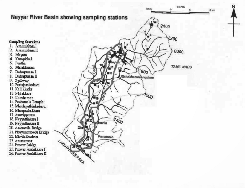
Figure 1: Monitoring station positions on the Neyyar river basin. We use the station locations and data within the encircled area.

The location of each monitoring station is specified by its geographical coordinates, that is, latitude and longitude. At each of these stations, measurements are taken for two variables: pH and phosphate which are used to measure the quality of water. For carrying out the analysis, that is, gathering information on the direct covariance and cross-covariance functions and parameters of the two responses, we use data from a single branch of the river with 17 stations (see the encircled region in Figure 1). We denote this branch of the river by $\mathcal{D}_{2}\;(\subseteq\mathbb{R}^{2})$ and in this case we have $n=17$. We denote the set of sampling points on this river branch by $\mathcal{S}_{2}=\{w_{1},\ldots,w_{17}\}\;(\subseteq\mathcal{D}_{2})$, where each $w_{i}=(latitude_{i},longitude_{i}),\,i=1,\ldots,17$. Let $w_{1}$ and $w_{17}$ respectively be the starting (station 6) and the end point (station 26) of the river branch, and suppose we assume $w_{i}$ is upstream of $w_{j}$ if $i<j$ for all $i,j=1,\ldots,17$.

The results that we obtained for determining optimal designs in earlier sections were based on one-dimensional inputs, that is, where the region of interest was denoted by $\mathcal{D}\subset\mathbb{R}$. In fact, without loss of generality we had assumed $\mathcal{D}=[0,1]$. So, we first use a transformation on our two-dimensional input sets $\mathcal{S}_{2}$ and $\mathcal{D}_{2}$ given by:

$$\varphi:\mathcal{D}_{2} \longrightarrow[0,1]$$

$$w \mapsto\dfrac{\mid\mid w-w_{1}\mid\mid}{\mid\mid w_{17}-w_{1}\mid\mid},$$

where $\mid\mid u-v\mid\mid$ is the geodesic stream distance between the two points $u$ and $v$ along the river and $u,v\in\mathcal{D}_{2}$. The geodesic distance is used to calculate distance on the earth’s surface and is discussed in Banerjee et al., (2014) in detail. The stream distance is the shortest distance between two locations on a stream, where the distance is computed along the stream (Ver Hoef et al.,, 2006). In this case it was not possible to calculate the exact stream distance using solely the coordinates of monitoring points. So, the stream distance between two adjacent points was approximated by the geodesic distance between the two points.

The transformed region of interest $\varphi(\mathcal{D}_{2})=\mathcal{D}_{1}=[0,1]$ and the set of sampling points $\varphi(\mathcal{S}_{2})=\mathcal{S}_{1}$ are one-dimensional. We had to constrain ourselves to a single branch of river as a single branch of river is connected and hence can be considered to be a one-dimensional object. For example, consider stations 10, 18 and 23 which are very close to the main branch, but if these points were included, then the transformation to a one-dimensional set would not work. The transformed set of observation points is given by $\mathcal{S}_{1}=\{x_{1},x_{2},\ldots,x_{17}\}$ where $\varphi(w_{i})=x_{i}$ for all $i=1,\ldots,17$. Also, by definition of the function $\varphi(\cdot)$ $x_{1}=0$, $x_{17}=1$ and $x_{i}<x_{j}$ for $i<j$, and $d_{i}=x_{i+1}-x_{i}$ for $i=1,\ldots,16$.

We took the pH level (a scalar with no units) as the primary variable $Z_{1}(\cdot)$, and phosphate concentration (measured in mg/l) as the secondary variable $Z_{2}(\cdot)$, with both the variables centered and scaled.

To investigate the covariance function and corresponding parameters we fitted a model by likelihood maximization, separately for each variable. Below we see Table 2, which was computed using the $likfit$ function with a constant mean (that is, corresponding to unknown mean) from the $geoR$ package (R-3.6.0 software). The likelihood values in Table 2 suggest that taking the random processes as a zero-mean process with an exponential variance structure and zero nugget effect is a reasonable choice for both variables. Using the information from the univariate analysis of pH and phosphate we next try to set up the appropriate bivariate simple cokriging model. Note that for both variables, we tried to fit a Gaussian covariance structure, however, the algorithm did not converge.

pH
Covariance Model	$C(h)=\sigma^{2}\rho(h)$	Log-Likelihood	Variance	Parameter ($\theta$, $\kappa$)	Nugget
Constant but unknown mean
Exponential	$\sigma^{2}exp(-\theta|h|)$	-20.28	0.85	16.95	0
Spherical	$\sigma^{2}\begin{cases}1-1.5h\theta+.5(h\theta)^{3},&\textit{ if }h<\dfrac{1}{\theta}\\ 0,&\text{otherwise}\end{cases}$	-20.74	0.96	7.90	0
Matern	$\sigma^{2}\dfrac{1}{2^{(\kappa-1)}\Gamma(\kappa)}(h\theta)^{\kappa}K_{\kappa}(h\theta)$	-20.15	0.83	(11.09,0.35)	0
Known mean equal to zero
Exponential	$\sigma^{2}exp(-\theta|h|)$	-20.29	0.85	17.12	0
phosphate
Covariance Model	$C(h)=\sigma^{2}\rho(h)$	Log-Likelihood	Variance	Parameter ($\theta$, $\kappa$)	Nugget
Constant but unknown mean
Exponential	$\sigma^{2}exp(-\theta|h|)$	-23.19	0.97	38.35	0
Spherical	$\sigma^{2}\begin{cases}1-1.5h\theta+.5(h\theta)^{3},&\textit{ if }h<\dfrac{1}{\theta}\\ 0,&\text{otherwise}\end{cases}$	-23.09	0.95	19.02	0
Matern	$\sigma^{2}\dfrac{1}{2^{(\kappa-1)}\Gamma(\kappa)}(h\theta)^{\kappa}K_{\kappa}(h\theta)$	-23.85	0.97	(0.01,0.003)	0
Known mean equal to zero
Exponential	$\sigma^{2}exp(-\theta|h|)$	-23.29	0.96	45.94	0

Table 2: Results of Likelihood Analysis of pH and Phosphate for Different Covariance Models

We consider $Z_{1}(\cdot)$ and $Z_{2}(\cdot)$ to have the exponential parameters $\theta$ and $\phi$, respectively. The results from Table 2 for pH and phosphate indicate a large difference between $\hat{\theta}$ and $\hat{\phi}$. Thus, it seems more appropriate to assume a generalized Markov-type bivariate covariance rather than proportional covariances in the bivariate cokriging model. Based on the assumption of normal errors, the log-likelihood function is:

$$l=-\dfrac{n}{2}log(2\pi)-\dfrac{1}{2}log[det(\boldsymbol{\Sigma})]-\dfrac{1}{2}\mathbf{Z}^{T}\boldsymbol{\Sigma}^{-1}\mathbf{Z},$$

where $\mathbf{Z}=(\mathbf{Z}_{1},\mathbf{Z}_{2})^{T}$, $\boldsymbol{\Sigma}=\begin{bmatrix}\boldsymbol{C}_{11}&\rho\boldsymbol{C}_{11}\\ \rho\boldsymbol{C}_{11}&\rho^{2}\boldsymbol{C}_{11}+(\sigma_{22}-\rho^{2}\sigma_{11})\boldsymbol{C}_{R}\end{bmatrix}$, and $\boldsymbol{C}_{R}$ is chosen to be the identity matrix.

Using the $optim$ function in (R-3.6.0 software) we find the MLEs to be $\hat{\theta}=17.12$, $\hat{\sigma_{11}}=0.85$, $\hat{\sigma_{22}}=0.94,$ $\hat{\rho}=.25$ and $l=-27.74$. The $likfit$ and $optim$ functions in R-3.6.0 were used for computations.

Illustration 6.1.

Relative efficiency when parameter values are known

The design given for the pilot monitoring network is denoted by $\boldsymbol{\xi}_{0}$, which is obtained by considering the 17 points on the river (encircled region) and applying the transformation $\varphi(\cdot)$. We computed $\boldsymbol{\xi}_{0}=(0.04,0.02,0.04,0.09,0.20,0.06,0.12,0.13,0.04,0.04,0.02,0.05,0.04,\\ 0.07,0.02,0.02)$. We also denoted the equispaced design by $\boldsymbol{\xi}^{\ast}$, where $(\boldsymbol{\xi}^{\ast})_{i}=\dfrac{1}{n-1}=\dfrac{1}{16}$ for all $i=1,\ldots,17$. The parameter values are taken to be the same as the maximum likelihood estimates.

Relative efficiency based on IMSPE of design $\boldsymbol{\xi}_{0}$ with respect to the optimal design $\boldsymbol{\xi}^{\ast}$ is defined as the ratio, $\dfrac{\text{IMSPE($\boldsymbol{\xi}^{\ast}$)}}{\text{IMSPE($\boldsymbol{\xi}_{0}$)}}$. For known parameters, using the expression of IMSPE in Theorem 5.2, the relative efficiency of the river network (or design) $\boldsymbol{\xi}_{0}$ is found to be 0.797. Similarly, for the SMSPE criterion we define the ratio as $\dfrac{\text{SMSPE($\boldsymbol{\xi}^{\ast}$)}}{\text{SMSPE($\boldsymbol{\xi}_{0}$)}}$. For the SMSPE criterion, using Theorem 5.1 the relative efficiency of the river network $\boldsymbol{\xi}_{0}$ is 0.524. Note that relative efficiency values in both cases indicate a sizable increase in prediction accuracy if equispaced designs were used instead.

Illustration 6.2.

Relative efficiency for unknown parameters

Consider, $\theta\sim Unif(\theta_{1},\theta_{2})$ for $0<\theta_{1}<\theta_{2}<\infty$, a common choice of prior for $\theta$ (see Stehlík et al., (2015)) and $\sigma_{11}\sim t(\cdot)$ for some density function $t(\cdot)$. Note we could have chosen any prior function for $\theta$ other than the uniform distribution as long as it had a finite support. The risks for the uniform prior are,

$$\mathcal{R}_{1}(\boldsymbol{\xi}) =E_{\sigma}\;\;\dfrac{1}{\theta_{2}-\theta_{1}}\dfrac{1}{d_{max}}\Bigg{[}2ln\dfrac{1+e^{-\theta_{2}d_{max}}}{1+e^{-\theta_{1}d_{max}}}+d_{max}(\theta_{2}-\theta_{1})\Bigg{]}$$ (36)

and,

$$\mathcal{R}_{2}(\boldsymbol{\xi}) =E_{\sigma}\;\;\Bigg{[}1-\dfrac{n-1}{\theta_{2}-\theta_{1}}\;\;ln\dfrac{\theta_{2}}{\theta_{1}}+\dfrac{1}{\theta_{2}-\theta_{1}}\sum_{i=1}^{n-1}ln\Big{(}\dfrac{e^{2\theta_{2}d_{i}}-1}{e^{2\theta_{2}d_{i}}}.\dfrac{e^{2\theta_{1}d_{i}}}{e^{2\theta_{1}d_{i}}-1}\Big{)}\Bigg{]},$$ (37)

where $\smash{\displaystyle\max_{i}}(d_{i})$ is written as $d_{max}$ and $E_{\sigma}=E_{t}[\sigma_{11}]$. The relative efficiency is then $\dfrac{{\mathcal{R}_{i}(\boldsymbol{\xi}^{\ast})}}{{\mathcal{R}_{i}(\boldsymbol{\xi}_{0})}},\,i=1,2$. Note, these risks in (36) and (37) would differ if we change the prior. However $\boldsymbol{\xi}^{\ast}$ would remain same.

Using $\hat{\theta}=17.12$, we choose $\theta_{1}$ and $\theta_{2}$ such that the mean of the interval is $\hat{\theta}$. Varying the range of values for $\theta_{1}$ and $\theta_{2}$, the relative risks are shown in the following Table 3.

$\theta_{1}$	$\theta_{2}$	$\mathcal{R}_{1}(\boldsymbol{\xi}^{\ast})/E_{\sigma}$	$\mathcal{R}_{1}(\boldsymbol{\xi}_{0})/E_{\sigma}$	$\dfrac{\mathcal{R}_{1}(\boldsymbol{\xi}^{\ast})}{\mathcal{R}_{1}(\boldsymbol{\xi}_{0})}$	$\mathcal{R}_{2}(\boldsymbol{\xi}^{\ast})/E_{\sigma}$	$\mathcal{R}_{2}(\boldsymbol{\xi}_{0})/E_{\sigma}$	$\dfrac{\mathcal{R}_{2}(\boldsymbol{\xi}^{\ast})}{\mathcal{R}_{2}(\boldsymbol{\xi}_{0})}$
16.62	17.62	0.489	0.933	0.524	0.332	0.434	0.766
16.12	18.12	0.489	0.933	0.524	0.332	0.433	0.766
15.12	19.12	0.489	0.932	0.525	0.332	0.433	0.766
12.12	22.12	0.486	0.923	0.527	0.330	0.430	0.768

Table 3: Relative risk of given design - IMSPE and SMSPE criterion

From Table 3, we note small changes in the relative efficiency for changes in $\theta_{1}$ and $\theta_{2}$, suggesting that the criterion is robust to changes in the prior information regarding $\theta$. This robustness persists when we change the values of $\hat{\theta}$. We also checked relative efficiencies for $\hat{\theta}=$ 7.12, 27.12 and 47.12, however the results are not shown here.

7 Concluding remarks

Multivariate kriging models are of particular practical interest in computer experiments, spatial and spatio-temporal applications. Very often, two or more correlated responses may be observed, and prediction from cokriging may improve prediction quality over kriging for each variable separately.

In this article, we identify a class of cross-covariance functions, which in fact includes many popularly used bivariate covariance functions, for which the cokriging estimator reduces to a kriging estimator. Thereafter, we address the problem of determining designs for some of these cokriging models. Since the designs are dependent on the covariance parameters, Bayesian designs are proposed. We prove that the locally and Bayesian optimal designs are both equispaced. Intuitively, this could be explained due to the fact that the locally optimal designs are equispaced for all the values of covariance parameters. So, when we mathematically find the Bayesian optimal designs, both are equispaced.

As a future extension, we are interested in determining optimal designs for universal cokriging models. However, as illustrated in Dette et al., (2008) and Dette et al., (2013), obtaining theoretical designs for such models is difficult. We have also come across situations in cokriging experiments where time and space (or multiple inputs) both may affect the responses. Thus, there is a need to extend optimal designs to cover such scenarios where the input space is a multidimensional grid of points.

Appendix A Appendix

Result A.1.

Consider two random functions $Z_{1}(\cdot)$ and $Z_{2}(\cdot)$ with respective covariance functions $\mathcal{C}_{ii}(\cdot)$ and spectral densities $s_{i}(\cdot)$ for $i=1,2$. Consider another valid correlation function $\mathcal{C}_{R}(\cdot)$ with spectral density $s_{R}(\cdot)$. Then, $\boldsymbol{\Sigma}$ as defined in (7) is a valid covariance matrix if and only if $(\sigma_{22}-\rho^{2}\sigma_{11})>0$.

Proof.

The cross-spectral density matrix $\boldsymbol{S}_{p}(u)$ is,

$$\boldsymbol{S}_{p}(u) =\begin{bmatrix}s_{1}(u)&\rho s_{1}(u)\\ \rho s_{1}(u)&\;\;\rho^{2}s_{1}(u)+(\sigma_{22}-\rho^{2}\sigma_{11})s_{R}(u)\end{bmatrix},u\in\mathbb{R}$$

with determinant $s_{1}(u)(\sigma_{22}-\rho^{2}\sigma_{11})s_{R}(u)$. Note, that the matrix $\boldsymbol{S}_{p}(u)$ is positive definite whenever $(\sigma_{22}-\rho^{2}\sigma_{11})>0$, as $s_{1}(\cdot)$ and $s_{R}(\cdot)$ correspond to the inverse Fourier transforms of the covariance functions $\mathcal{C}_{11}(\cdot)$ and $\mathcal{C}_{R}(\cdot)$, respectively. Using the criterion of Cramér, (1940), $\boldsymbol{\Sigma}$ is then a valid covariance matrix if and only if $(\sigma_{22}-\rho^{2}\sigma_{11})>0$. ∎

Appendix B Appendix

We list down some of the key matrices, vectors and their decomposition required for proving results in Lemma 5.1 and Theorems 5.1, 5.2, 5.5 and 5.6. In this article, we have used an exponential covariance matrix $\boldsymbol{P}$, where

$$\boldsymbol{P} =\begin{bmatrix}1&e^{-\theta|x_{1}-x_{2}|}&\;\;\;\;\;\;\;&\ldots&e^{-\theta|x_{1}-x_{n}|}\\ e^{-\theta|x_{2}-x_{1}|}&1&\;\;\;\;\;\;\;&\ldots&e^{-\theta|x_{2}-x_{n}|}\\ .&.&\;\;\;\;\;\;\;&\ldots&.\\ .&.&\;\;\;\;\;\;\;&\ldots&.\\ .&.&\;\;\;\;\;\;\;&\ldots&.\\ e^{-\theta|x_{n}-x_{1}|}&e^{-\theta|x_{n}-x_{2}|}&\;\;\;\;\;\;\;&\ldots&1\end{bmatrix}.$$

Considering matrices $\boldsymbol{L}$ and $\boldsymbol{D}$, as in Antognini and Zagoraiou, (2010),

$$\boldsymbol{L} =\begin{bmatrix}1&0&0&.&.&.&0\\ e^{-\theta d_{1}}&1&0&.&.&.&0\\ e^{-\theta\Sigma^{2}_{i=1}d_{i}}&e^{-\theta d_{2}}&1&.&.&.&0\\ .&.&.&.&.&&\\ .&.&.&.&..&&\\ e^{-\theta\Sigma^{n-1}_{i=1}d_{i}}&e^{-\theta\Sigma^{n-1}_{i=2}d_{i}}&e^{-\theta\Sigma^{n-1}_{i=3}d_{i}}&.&.&.&1\\ \end{bmatrix}\text{ and }\boldsymbol{D}=diag(1,1-e^{-2\theta d_{1}},\ldots,1-e^{-2\theta d_{n-1}}),$$

we wrote $\boldsymbol{P}=\boldsymbol{L}\boldsymbol{D}\boldsymbol{L}^{T}$. Thus,

$$\boldsymbol{P}^{-1} =(\boldsymbol{D}^{-1/2}\boldsymbol{L}^{-1})^{T}(\boldsymbol{D}^{-1/2}\boldsymbol{L}^{-1}),$$ (38)

where

$$\boldsymbol{P}^{-1}= \begin{bmatrix}\dfrac{1}{1-e^{-2\theta d_{1}}}&\dfrac{-e^{\theta d_{1}}}{1-e^{-2\theta d_{1}}}&&.&.&.&0\\ \dfrac{-e^{\theta d_{1}}}{1-e^{-2\theta d_{1}}}&\dfrac{1}{1-e^{-2\theta d_{1}}}+\dfrac{e^{-2\theta d_{2}}}{1-e^{-2\theta d_{2}}}&&0&.&.&0\\ .\\ .\\ .\\ 0&.&&0&.&\dfrac{1}{1-e^{-2\theta d_{n-2}}}+\dfrac{e^{-2\theta d_{n-1}}}{1-e^{-2\theta d_{n-1}}}&\dfrac{-e^{\theta d_{n-1}}}{1-e^{-2\theta d_{n-1}}}\\ 0&0&&.&.&\dfrac{-e^{\theta d_{n-1}}}{1-e^{-2\theta d_{n-1}}}&\dfrac{1}{1-e^{-2\theta d_{n-1}}}\end{bmatrix}.$$ (39)

Appendix C Appendix

Here, we evaluate $\Omega{(\boldsymbol{\xi})}=\boldsymbol{1}_{n}^{T}\boldsymbol{P}^{-1}\boldsymbol{1}_{n}$ and show that $\dfrac{1}{\Omega{(\boldsymbol{\xi})}}$ is a Schur-convex function, which is minimized for an equispaced partition. Using equation (38) from B, we write,

$$\boldsymbol{1}_{n}^{T}\boldsymbol{P}^{-1}\boldsymbol{1}_{n} =(\boldsymbol{D}^{-1/2}\boldsymbol{L}^{-1}\boldsymbol{1}_{n})^{T}(\boldsymbol{D}^{-1/2}\boldsymbol{L}^{-1}\boldsymbol{1}_{n})=\boldsymbol{\gamma}^{T}\boldsymbol{\gamma},$$

where

$$\boldsymbol{\gamma}^{T} =(\boldsymbol{D}^{-1/2}\boldsymbol{L}^{-1}\boldsymbol{1}_{n})^{T}\;\;=\Big{(}1,\dfrac{1-e^{-\theta d_{1}}}{\sqrt{(1-e^{-2\theta d_{1}})}},\ldots,\dfrac{1-e^{-\theta d_{n-1}}}{\sqrt{(1-e^{-2\theta d_{n-1}})}}\Big{)}.$$

Hence we have,

$$\boldsymbol{1}_{n}^{T}\boldsymbol{P}^{-1}\boldsymbol{1}_{n} =1+\sum_{i=1}^{n-1}\dfrac{e^{\theta d_{i}}-1}{e^{\theta d_{i}}+1}.$$

As without loss of generality we assumed $\sum_{i=1}^{n-1}d_{i}=1$, therefore

$$\boldsymbol{1}_{n}^{T}\boldsymbol{P}^{-1}\boldsymbol{1}_{n} =\sum_{i=1}^{n-1}\Big{[}d_{i}+\dfrac{e^{\theta d_{i}}-1}{e^{\theta d_{i}}+1}\Big{]}.$$

Using the above expression we write

$$\Omega{(\boldsymbol{\xi})} =\sum_{i=1}^{n-1}\omega(d_{i}),\text{ where, }\omega(d)=d+\dfrac{e^{\theta d}-1}{e^{\theta d}+1}.$$ (40)

Next, differentiating $\Omega{(\boldsymbol{\xi})}$ with respect to $d_{i}$ we obtain

$$\dfrac{\partial\Omega{(\boldsymbol{\xi})}}{\partial d_{i}} =1+\dfrac{2\theta e^{\theta d_{i}}}{(e^{\theta d_{i}}+1)^{2}},$$

$$\dfrac{\partial^{2}\Omega{(\boldsymbol{\xi})}}{\partial d_{i}^{2}} =\dfrac{2\theta^{2}e^{\theta d_{i}}(1-e^{\theta d_{i}})}{(1+e^{\theta d_{i}})^{3}}<0.$$ (41)

Hence, for $Q(\boldsymbol{\xi})=\dfrac{1}{\Omega{(\boldsymbol{\xi})}}$ we have

$$\dfrac{\partial Q(\boldsymbol{\xi})}{\partial d_{l}}-\dfrac{\partial Q(\boldsymbol{\xi})}{\partial d_{k}} =\dfrac{1}{(\Omega{(\boldsymbol{\xi})})^{2}}\Big{[}\dfrac{\partial\omega(d_{k})}{\partial d_{k}}-\dfrac{\partial\omega(d_{l})}{\partial d_{l}}\Big{]}\text{ for }k,l=1,\ldots,n-1.$$ (42)

Note that $Q(\cdot)$ is permutation invariant of $d_{i}$’s . Also, $\dfrac{\partial Q(\boldsymbol{\xi})}{\partial d_{l}}>\dfrac{\partial Q(\boldsymbol{\xi})}{\partial d_{k}}\text{ for }d_{l}>d_{k}$, where $k,l=1,\ldots,n-1$ (using equations (41) and (42)). So, we can say that $Q(\cdot)$ is a Schur-convex function (from Theorem A.4 in Marshall et al., (1979)) and hence it is minimized for an equispaced design, that is $d_{i}=\dfrac{1}{n-1}$ for all $i$.

Appendix D Appendix

In this part, we look at some matrix and vector decompositions used for proving results involving the $SMSPE$ for simple and ordinary cokriging models.

Consider $x_{0}\in[x_{i},x_{i+1}]$ for some $i=1,\ldots,n-1$, recall that $a=x_{0}-x_{i}$ and let an $n\times n$ diagonal matrix, $\boldsymbol{E}=diag\begin{pmatrix}e^{-\theta\sum_{l=1}^{i-1}d_{l}},&e^{-\theta\sum_{l=2}^{i-1}d_{l}},&\ldots 1,&1,&e^{-\theta d_{i+1}},&\ldots e^{-\theta\sum_{l=i+1}^{n-1}d_{l}}\end{pmatrix}$, such that $(\boldsymbol{E})_{ii}=1$ and $(\boldsymbol{E})_{i+1\;i+1}=1$. Also, consider two vectors of length $n$, $\boldsymbol{e}_{1}=\begin{pmatrix}1&1&\ldots 1&0&0&\ldots 0\end{pmatrix}$ and $\boldsymbol{e}_{2}=\begin{pmatrix}0&0&\ldots 0&1&1&\ldots 1\end{pmatrix}$, such that $(\boldsymbol{e}_{1})_{i}=1$ and $(\boldsymbol{e}_{1})_{i+1}=0$, and $(\boldsymbol{e}_{2})_{i}=0$ and $(\boldsymbol{e}_{2})_{i+1}=1$. Then, we may write $\boldsymbol{\sigma}_{p0}$ as,

$$\boldsymbol{\sigma}_{p0} =\boldsymbol{E}\;\;\Big{[}e^{-\theta a}\boldsymbol{e}_{1}+e^{-\theta(d_{i}-a)}\boldsymbol{e}_{2}\Big{]}.$$ (43)

Using the $n\times 1$ vectors $\boldsymbol{u}_{1},\boldsymbol{u}_{2},\boldsymbol{v}_{1}$, and $\boldsymbol{v}_{2}$ defined as:

$$\boldsymbol{u}_{1}^{T} =\begin{pmatrix}e^{-\theta\sum_{l=1}^{i-1}d_{l}},&e^{-\theta\sum_{l=2}^{i-1}d_{l}},&\ldots&&\;\;,1^{i^{th}pos},&0,&0,\ldots&\;\;\;\;\;\;\;\;\;\;\;\;\;\;\;\;\;\;\;\;\;\;\;\;\;\;\;\;\;\;&&\ldots\ldots,0\end{pmatrix},$$

$$\boldsymbol{u}_{2}^{T} =\begin{pmatrix}0,&0,\ldots&\;\;\;\;\;\;\;\;\;\;\;\;\;\;\;\;\;\;\;\;\;\;\;\;&&\ldots,0\;\;\;\;&,1^{(i+1)^{th}pos},&e^{-\theta d_{i+1}},&&&\;\ldots\ldots,e^{-\theta\sum_{l=i+1}^{n-1}d_{l}}\end{pmatrix},$$

$$\boldsymbol{v}_{1}^{T} =\begin{pmatrix}0,&0,\ldots&&\;\;\;&,0^{(i-1)^{th}pos},&\dfrac{1}{1-e^{-2\theta d_{i}}},&\dfrac{-e^{-\theta d_{i}}}{1-e^{-2\theta d_{i}}},&0,&\;\;\;\;\;\;\;\;\;\;\;\;\;\;\;\;\;&\;\;\ldots\ldots\ldots,0\end{pmatrix},$$

$$\boldsymbol{v}_{2}^{T} =\begin{pmatrix}0,&0,\ldots&&\;\;\;&,0^{(i-1)^{th}pos},&\dfrac{-e^{-\theta d_{i}}}{1-e^{-2\theta d_{i}}},&\dfrac{1}{1-e^{-2\theta d_{i}}},&0,&\;\;\;\;\;\;\;\;\;\;\;\;\;\;\;\;\;\;\;&\ldots\ldots\ldots,0\end{pmatrix}$$

and $\boldsymbol{\sigma}_{p0}$ from (43) and $\boldsymbol{P}^{-1}$ from (39) we obtain:

$$\boldsymbol{\sigma}_{p0} =e^{-\theta a}\boldsymbol{u}_{1}+e^{-\theta(d_{i}-a)}\boldsymbol{u}_{2},$$ (44)

$$\boldsymbol{P}^{-1}\boldsymbol{\sigma}_{p0} =e^{-\theta a}\boldsymbol{v}_{1}+e^{-\theta(d_{i}-a)}\boldsymbol{v}_{2},$$ (45)

$$\boldsymbol{\sigma}_{p0}^{T}\boldsymbol{P}^{-1}\boldsymbol{\sigma}_{p0} =\dfrac{e^{-2\theta a}-2e^{-2\theta d_{i}}+e^{-2\theta(d_{i}-a)}}{1-e^{-2\theta d_{i}}},\text{ and }$$ (46)

$$\boldsymbol{1}_{n}^{T}\boldsymbol{P}^{-1}\boldsymbol{\sigma}_{p0} =\dfrac{e^{-\theta a}+e^{-\theta(d_{i}-a)}}{1+e^{-\theta d_{i}}}.$$ (47)

Appendix E Appendix

We show here that if $x_{0}\in[x_{i},x_{i+1}]$ for some $i=1,...,n-1$ then the $MSPE_{sk}(x_{0})$ is maximized at $x_{0}=x_{i}+\dfrac{d_{i}}{2}$. From Lemma 5.1, we have

$$MSPE_{sk}(x_{0}) =\sigma_{11}\dfrac{\left(1-e^{-2\theta a}\right)\left(1-e^{-2\theta(d_{i}-a)}\right)}{\left(1-e^{-2\theta d_{i}}\right)}.$$ (48)

Since, $x_{0}\in[x_{i},x_{i+1}]$ and $a=x_{0}-x_{i}$, therefore $a\in[0,d_{i}]$ for $i=1,\ldots,n-1$. Now, consider the function

$$W_{i}: \;\;[0,d_{i}]\;\to\mathbb{R}\;\;\;\;\;\;\;\;\;\;\;\;\;$$

$$a \mapsto\dfrac{\left(1-e^{-2\theta a}\right)\left(1-e^{-2\theta(d_{i}-a)}\right)}{\left(1-e^{-2\theta d_{i}}\right)}.$$

Differentiating $W_{i}(\cdot)$ with respect to $a$ we get,

$$\dfrac{dW_{i}(a)}{da}=\dfrac{2\theta\left(e^{-2\theta a}-e^{-2\theta(d_{i}-a)}\right)}{\left(1-e^{-2\theta d_{i}}\right)},$$

where,

$$\dfrac{dW_{i}(a)}{da}\Bigg{|}_{a=d_{i}/2}=0,$$ (49)

and

$$\dfrac{d^{2}W_{i}(a)}{da^{2}} =\dfrac{-4\theta^{2}\left(e^{-2\theta a}+e^{-2\theta(d_{i}-a)}\right)}{\left(1-e^{-2\theta d_{i}}\right)}<\;0.$$ (50)

From equations (49) and (50), for $x_{0}\in[x_{i},x_{i+1}]$, $W_{i}(\cdot)$ is maximized at $d_{i}/2$ or equivalently $MSPE(x_{0})$ over $[x_{i},x_{i+1}]$ is maximized at $x_{0}=x_{i}+\dfrac{d_{i}}{2}$. Hence,

$$\sup_{x_{0}\in[x_{i},x_{i+1}]}MSPE(x_{0})= W_{i}(d_{i}/2)$$

$$= \sigma_{11}\frac{1-e^{-\theta d_{i}}}{1+e^{-\theta d_{i}}}.$$ (51)

Appendix F Appendix

We prove that $IMSPE_{sk}$ is a Schur-convex function. First note, $IMSPE$ is a symmetric function, that is, it is permutation invariant in the $d_{i}$’s. Next we find $\dfrac{\partial IMSPE}{\partial d_{i}}$ and show that it is an increasing function in the $d_{i}$’s for $i=1,\ldots,n$;

$$\dfrac{\partial\phi(d)}{\partial d} =\dfrac{e^{2\theta d}-1-2\theta de^{2\theta d}}{(e^{2\theta d}-1)^{2}}\text{ is an increasing function in }d\in(0,1)$$ (52)

$$\text{since, }\dfrac{\partial^{2}\phi(d)}{\partial d^{2}} =\dfrac{4\theta e^{2\theta d}}{{(e^{2\theta d}-1)}^{3}}(1+\theta d+e^{2\theta d}(\theta d-1))$$

$$=\dfrac{4\theta e^{2\theta d}}{{(e^{2\theta d}-1)}^{3}}\;\;p(d,\theta)\geq 0,\text{ for }d\in(0,1),$$

where $p(d,\theta)=(1+\theta d+e^{2\theta d}(\theta d-1))\geq 0$ and $\frac{\partial p(d)}{\partial d}|_{d=0}=\frac{\partial^{2}p(d)}{\partial d^{2}}|_{d=0}=0$ and $\frac{\partial^{2}p(d)}{\partial d^{2}}>0$ for $d\in(0,1]$.
As, $\dfrac{\partial IMSPE}{\partial d_{i}}=2\sigma_{11}\dfrac{\partial\phi(d_{i})}{\partial d_{i}}$ for $i=1,\ldots,n-1$, using (52) we can say:

$$\dfrac{\partial IMSPE}{\partial d_{k}}\leq\dfrac{\partial IMSPE}{\partial d_{l}}\;\;\;\text{ for any }d_{k}\leq d_{l}.\\$$ (53)

Thus, using Theorem A.4 from Marshall et al., (1979), we can say that $IMSPE$ is Schur-convex.

Appendix G Appendix

We show that for $x_{0}\in[x_{i},x_{i+1}]$ for some $i=1,\ldots,n-1$, $\smash{\displaystyle\sup_{x_{0}\in[x_{i},x_{i+1}]}}\Big{(}1-\boldsymbol{1}_{n}^{T}\boldsymbol{P}^{-1}\boldsymbol{\sigma}_{p0}\Big{)}^{2}$ is attained at $x_{0}=x_{i}+\dfrac{d_{i}}{2}$. From (47) in D we have,

$$\boldsymbol{1}_{n}^{T}\boldsymbol{P}^{-1}\boldsymbol{\sigma}_{p0} =\dfrac{e^{-\theta a}+e^{-\theta(d_{i}-a)}}{1+e^{-\theta d_{i}}}.$$

As $a\in[0,d_{i}]$, defining the function $U_{i}(\cdot)$ such that,

$$U_{i}: [0,d_{i}]\to\mathbb{R}$$

$$a \mapsto\Bigg{(}1-\dfrac{e^{-\theta a}+e^{-\theta(d_{i}-a)}}{1+e^{-\theta d_{i}}}\Bigg{)}^{2}$$

we obtain

$$\dfrac{dU_{i}(a)}{da}=-2\theta\underbrace{\Bigg{(}1-\dfrac{e^{-\theta a}+e^{-\theta(d_{i}-a)}}{1+e^{-\theta d_{i}}}\Bigg{)}}_{TermI}\underbrace{\Bigg{(}\dfrac{-e^{-\theta a}+e^{-\theta(d_{i}-a)}}{1+e^{-\theta d_{i}}}\Bigg{)}}_{TermII}$$ (54)

where

$$\dfrac{dU_{i}(a)}{da}\Bigg{|}_{a=d_{i}/2}=0$$ (55)

and

$$\dfrac{d^{2}U_{i}(a)}{da^{2}}=-4\theta^{2}\Big{(}\dfrac{1-e^{-\theta d_{i}/2}}{1+e^{-\theta d_{i}}}\Big{)}^{2}e^{-\theta d_{i}}<0.$$ (56)

From (55) and (56) we see $U_{i}(\cdot)$ attains a local maxima at $a=\dfrac{d_{i}}{2}$ and $U_{i}(\dfrac{d_{i}}{2})=\Big{(}1-\dfrac{2e^{-\theta d_{i}/2}}{1+e^{-\theta d_{i}}}\Big{)}^{2}>0$. To find the point of maxima $a=d_{i}/2$ we set $Term\;II$ in (54) equal to zero. Any other point $a_{1}$ at which $U^{\prime}(a_{1})=0$ is obtained by setting $Term\;I$ equal to zero; however, those points could not be the maxima as $U_{i}(a_{1})$ is zero.
Hence, we have shown that $\smash{\displaystyle\sup_{a\in[0,d_{i}]}}U_{i}(a)=\smash{\displaystyle\sup_{x_{0}\in[x_{i},x_{i+1}]}}\Big{(}1-\boldsymbol{1}_{n}^{T}\boldsymbol{P}^{-1}\boldsymbol{\sigma}_{p0}\Big{)}^{2}$ is attained at $a=\dfrac{d_{i}}{2}$ or $x_{0}=x_{i}+\dfrac{d_{i}}{2}$ for some $i=1,\ldots,n-1$, which is the mid-point of the interval $[x_{i},x_{i+1}]$.

Hence, we obtain

$$\sup_{x_{0}\in[x_{i},x_{i+1}]}\Big{(}1-\boldsymbol{1}_{n}^{T}\boldsymbol{P}^{-1}\boldsymbol{\sigma}_{p0}\Big{)}^{2} =U_{i}(\dfrac{d_{i}}{2})=\Big{(}1-\dfrac{2e^{-\theta d_{i}/2}}{1+e^{-\theta d_{i}}}\Big{)}^{2}$$ (57)

Funding

This project is funded by IITB-Monash Research Academy, India.
The work of S. Mukhopadhyay was supported by the Science and Research Engineering Board (Department of Science and Technology, Government of India) [File Number: EMR/2016/005142].

Correspondence

Prof. Siuli Mukhopadhyay,
Department of Mathematics, Indian Institute of Technology Bombay,
Mumbai, Maharashtra, 400076, India
email - siuli@math.iitb.ac.in

References

• Antognini and Zagoraiou, (2010) Antognini, A.ย B. and Zagoraiou, M. (2010). Exact optimal designs for computer experiments via kriging metamodelling. Journal of Statistical Planning and Inference, 140:2607โ€“2617.
• Banerjee etย al., (2014) Banerjee, S., Carlin, B.ย P., and Gelfand, A.ย E. (2014). Hierarchical Modeling and Analysis for Spatial Data. Chapman and Hall/CRC.
• Baran etย al., (2013) Baran, S., Sikolya, K., and Stehlรญk, M. (2013). On the optimal designs for the prediction of ornstein-uhlenbeck sheets. Statistics & Probability Letters, 83:1580โ€“1587.
• Baran and Stehlรญk, (2015) Baran, S. and Stehlรญk, M. (2015). Optimal designs for parameters of shifted ornstein-uhlenbeck sheets measured on monotonic sets. Statistics & Probability Letters, 99:114โ€“124.
• Bueso etย al., (1999) Bueso, M., Angulo, J., Cruz-Sanjulian, J., and Garcรญa-Arรณstegui, J. (1999). Optimal spatial sampling design in a multivariate framework. Mathematical Geology, 31:507โ€“525.
• Caselton and Zidek, (1984) Caselton, W.ย F. and Zidek, J.ย V. (1984). Optimal monitoring network designs. Statistics & Probability Letters, 2:223โ€“227.
• Chaloner and Larntz, (1989) Chaloner, K. and Larntz, K. (1989). Optimal bayesian design applied to logistic regression experiments. Journal of Statistical Planning and Inference, 21:191โ€“208.
• Chiles and Delfiner, (2009) Chiles, J.-P. and Delfiner, P. (2009). Geostatistics: Modeling Spatial Uncertainty. John Wiley & Sons.
• Cramรฉr, (1940) Cramรฉr, H. (1940). On the theory of stationary random processes. Annals of Mathematics, 41:215โ€“230.
• Dette etย al., (2008) Dette, H., Kunert, J., and Pepelyshev, A. (2008). Exact optimal designs for weighted least squares analysis with correlated errors. Statistica Sinica, 18:135โ€“54.
• Dette etย al., (2013) Dette, H., Pepelyshev, A., and Zhigljavsky, A. (2013). Optimal design for linear models with correlated observations. The Annals of Statistics, 41:143โ€“176.
• Dette and Sperlich, (1996) Dette, H. and Sperlich, S. (1996). Some applications of stieltjes transforms in the construction of optimal designs for nonlinear regression models. Computational Statistics & Data Analysis, 21:273โ€“292.
• Diggle and Lophaven, (2006) Diggle, P. and Lophaven, S. (2006). Bayesian geostatistical design. Scandinavian Journal of Statistics, 33:53โ€“64.
• Genton and Kleiber, (2015) Genton, M.ย G. and Kleiber, W. (2015). Cross-covariance functions for multivariate geostatistics. Statistical Science, 30:147โ€“163.
• Journel, (1999) Journel, A.ย G. (1999). Markov models for cross-covariances. Mathematical Geology, 31:955โ€“964.
• Kiselโ€™รกk and Stehlรญk, (2008) Kiselโ€™รกk, J. and Stehlรญk, M. (2008). Equidistant and d-optimal designs for parameters of ornstein-uhlenbeck process. Statistics & Probability Letters, 78:1388โ€“1396.
• Le and Zidek, (1994) Le, N. and Zidek, J. (1994). Network designs for monitoring multivariate random spatial fields. Recent Advances in Statistics and Probability, page 191โ€“206.
• Li and Zimmerman, (2015) Li, J. and Zimmerman, D.ย L. (2015). Model-based sampling design for multivariate geostatistics. Technometrics, 57:75โ€“86.
• Madani and Emery, (2019) Madani, N. and Emery, X. (2019). A comparison of search strategies to design the cokriging neighborhood for predicting coregionalized variables. Stochastic Environmental Research and Risk Assessment, 33:183โ€“199.
• Marshall etย al., (1979) Marshall, A.ย W., Olkin, I., and Arnold, B.ย C. (1979). Inequalities: Theory of Majorization and Its Applications. Springer.
• Myers, (1983) Myers, D.ย E. (1983). Estimation of linear combinations and co-kriging. Journal of the International Association for Mathematical Geology, 15:633โ€“637.
• Myers, (1991) Myers, D.ย E. (1991). Pseudo-cross variograms, positivedefiniteness, and cokriging. Mathematical Geology, 23:805โ€“816.
• Mylona etย al., (2014) Mylona, K., Goos, P., and Jones, B. (2014). Optimal design of blocked and split-plot experiments for fixed effects and variance component estimation. Technometrics, 56:132โ€“144.
• Protter etย al., (2012) Protter, M.ย H., Charlesย Jr, B., etย al. (2012). Intermediate calculus. Springer Science & Business Media.
• Santner etย al., (2010) Santner, T.ย J., Williams, B.ย J., Notz, W.ย I., and Williams, B.ย J. (2010). The Design and Analysis of Computer Experiments. Springer.
• Sikolya and Baran, (2020) Sikolya, K. and Baran, S. (2020). On the optimal designs for the prediction of complex ornstein-uhlenbeck processes. Communications in Statistics-Theory and Methods, 49:4859โ€“4870.
• Singh and Mukhopadhyay, (2019) Singh, R. and Mukhopadhyay, S. (2019). Exact bayesian designs for count time series. Computational Statistics & Data Analysis, 134:157โ€“170.
• Singh and Mukhopadhyay, (2016) Singh, S.ย P. and Mukhopadhyay, S. (2016). Bayesian crossover designs for generalized linear models. Computational Statistics & Data Analysis, 104:35โ€“50.
• Stehlรญk etย al., (2015) Stehlรญk, M., Lรณpez-Fidalgo, J., Casero-Alonso, V., and Bukina, E. (2015). Robust integral compounding criteria for trend and correlation structures. Stochastic Environmental Research and Risk Assessment, 29:379โ€“395.
• Subramanyam and Pandalai, (2004) Subramanyam, A. and Pandalai, H. (2004). On the equivalence of the cokriging and kriging systems. Mathematical Geology, 36:507โ€“523.
• Verย Hoef and Cressie, (1993) Verย Hoef, J.ย M. and Cressie, N. (1993). Multivariable spatial prediction. Mathematical Geology, 25:219โ€“240.
• Verย Hoef etย al., (2006) Verย Hoef, J.ย M., Peterson, E., and Theobald, D. (2006). Spatial statistical models that use flow and stream distance. Environmental and Ecological statistics, 13:449โ€“464.
• Wackernagel, (2003) Wackernagel, H. (2003). Multivariate Geostatistics: An Introduction with Applications. Springer Science & Business Media.
• Woods and Vanย de Ven, (2011) Woods, D.ย C. and Vanย de Ven, P. (2011). Blocked designs for experiments with correlated non-normal response. Technometrics, 53:173โ€“182.
• Zagoraiou and Antognini, (2009) Zagoraiou, M. and Antognini, B. (2009). Optimal designs for parameter estimation of the ornsteinโ€“uhlenbeck process. Applied Stochastic Models in Business and Industry, 25:583โ€“600.
• Zimmerman, (2006) Zimmerman, D.ย L. (2006). Optimal network design for spatial prediction, covariance parameter estimation, and empirical prediction. Environmetrics: The Official Journal of the International Environmetrics Society, 17:635โ€“652.