Improving Vertical Positioning Accuracy with the Weighted Multinomial Logistic Regression Classifier

Abstract

In this paper, a method of improving vertical positioning accuracy with the Global Positioning System (GPS) information and barometric pressure values is proposed. Firstly, we clear null values for the raw data collected in various environments, and use the 3$\sigma$-rule to identify outliers. Secondly, the Weighted Multinomial Logistic Regression (WMLR) classifier is trained to obtain the predicted altitude of outliers. Finally, in order to verify its effect, we compare the Multinomial Logistic Regression (MLR) method, the WMLR method, and the Support Vector Machine (SVM) method for the cleaned dataset which is regarded as the test baseline. The numerical results show that the vertical positioning accuracy is improved from 5.9 meters (the MLR method), 5.4 meters (the SVM method) to 5 meters (the WMLR method) for 67% test points.

1 Introduction

In recent years, the performance of the Global Positioning System (GPS) is excellent in outdoor environments RGG2015 . When users are outdoors, their locations can be obtained accurately through GPS. However, the GPS signals are blocked by the buildings and other obstacles, which result in large indoor positioning errors. Thus, the indoor positioning accuracy is often challenged, especially in the vertical direction. In the meantime, the space that we are living in is filled with many high-rise buildings and our most activities are indoors. Considering the practical requirement and the poor indoor positioning performance, researchers have tried many methods to improve the vertical positioning accuracy, such as the WiFi-based localization technology DZYXKY2018 ; LLH2017 ; ZHLJX2016 and the barometer-based positioning technology XWJC2015 .

On the other hand, the GPS chip has been embedded in the most mobile terminals, which provides the location and timing information such as time, latitude, longitude, speed and altitude. Therefore, based on the GPS information, many researchers put forward some effective methods to improve the positioning accuracy of the low-cost GPS about 4 meters to 10 meters in several experiments IK2014 . Huang and Tsai propose an approach to calibrate the GPS position by using the context awareness technique from the pervasive computing and improve the positioning accuracy of GPS effectively HT2008 . The machine learning techniques are applied to assess and improve the GPS positioning accuracy under the forest canopy in ORMMS2011 .

In this paper, we provide another machine learning technique ALTMY2018 ; AASMGK2019 ; AZISYDML2019 based on the Multinomial Logistic Regression (MLR) method KS2016 ; MGB2008 for the vertical positioning problem. The research data are measured by many different user equipments and provided by Huawei Technologies Company, some data of which include the GPS three-dimensional information and the barometric pressure values, and Some data of which miss the GPS information or the barometric pressure values. We preprocess the research data firstly. Consequently, we identify the abnormal data with the $3\sigma$-rule and clear them. Meanwhile, some noises arise from the inaccurate data records and the different reference standards of different kinds of user equipments. These intrinsic noises lead to the poor distribution law between the air pressure and the corresponding altitude. In order to overcome these noise effects, we convert this vertical positioning problem into a classification problem and revise the weighted MLR method to improve its vertical positioning accuracy. Finally, in order to verify the effect of the Weighted Multinomial Logistic Regression (WMLR) method, we compare the MLR method, the WMLR method, and the Support Vector Machine (SVM) method CL2001 ; CL2013 ; CTS2017 for this vertical positioning problem. The numerical results show that the vertical positioning accuracy of the cleaned data is improved from 5.9 meters (the MLR method), 5.4 meters (the SVM method) to 5 meters (the WMLR method) for 67% test points.

The rest of the paper is organized as follows. In section 2, some related works are discussed. In section 3, we describes the methodology of the data cleaning, the outlier detection and the data correction based on the WMLR classifier. In section 4, we describe the data source and compare the MLR method, the WMLR method and the SVM method for the cleaned data which is regarded as the test baseline. The promising numerical results are also reported. Finally, some conclusions and the further works are discussed in section 5.

2 Related works

In the field of improving the indoor vertical positioning accuracy, many studies have been conducted. The related works can be roughly divided into two categories: the Received Signal Strength Strength Indication (RSSI) based methods and the barometric pressure based methods.

The RSSI of the Wi-Fi and the cellular network based methods use the collected the RSSI and build the database of the fingerprints for the floor positioning BSHL2016 ; WLSL2014 ; ZLC2012 . Some researchers consider the locations of the Wi-Fi access points to determine the floor GBRB2014 . In BSHL2016 , the experimental data are collected from one or two buildings and the collecting device is fixed. They use the collected RSSI information and the pressure data to estimate the floor. In those papers, since the RSSI information is local, when the experimental environment changes, the training data need to be collected by hand and the discriminant parameters need to be trained again.

Since there are many Wi-Fi access points distributed in a crowded indoor environment and the wall cannot completely obstruct the signals, the signal interference and fluctuation of different floors will result in the inaccurate estimation. Some researchers propose the barometric altimetry for the floor determination. In XWJC2015 , Xia et al. give a method based on the multiple reference barometers for the floor positioning in buildings and their method can give an accurate floor level. The disadvantages of their method are that the height thresholds should be given in the floor determination and they are sensitive to the local pressure conditions.

In CTS2017 , Chriki et al. use the SVM method based on the RSSI measurements for the zoning localization problem. In ALTMY2018 , Adege et al. propose an outdoor and indoor positioning method based on the hybrid of SVM and deep neural network algorithms according to the RSSI of the Wi-Fi. Since the SVM method only considers the support vector and the few points which are most relevant are used to make the classification, its classification result may be ineffective when the level of noise is high. The positioning method based on the deep neural network ALTMY2018 ; HLL2017 requires a very large amount of data to perform better than other techniques, and it requires expensive GPUs and multiple devices to train complex models. The MLR method considers all training data points which smooth the noise such that the MLR method can handle the high level of noise of the training data. Furthermore, the MLR method can be used to handle the large scale problem K2019 . Therefore, in consideration of the performance gain of the weighted positioning algorithm LLH2017 , we choose the MLR method with the weighted technique as the vertical positioning method based on the GPS and barometric pressure information of the user equipments.

3 The methodology

Our positioning method is composed of several stages, including the data cleaning, the outlier detection, the data correction and the prediction of vertical altitude for the test feature vector. We described these procedures in the following subsections.

3.1 Data cleaning

The raw dataset is measured at different places with different user equipments. In the dataset, many data miss the air pressure values due to some mobile devices without the barometers. We delete these data of the missing air pressure values firstly. Additionally, there are some abnormal data which deviate too far from the average value of the dataset and it is shown as follows. Assume that an average sea level pressure is 1013.25 hPa and the corresponding temperature is 15^∘C, then the air pressure value and its corresponding altitude have the following relationship ZF2014 :

$$h=44330.8-4946.54p^{0.1902632},$$ (1)

where the unit of altitude $h$ is meter, and the unit of the air pressure value $p$ is hpa. From formula (1), it is not difficult to find that the barometric pressure value and the corresponding altitude are the inverse relationship. However, from Fig. 1, we find that the distribution between the air pressure values and the corresponding altitudes of the given data is irregular. Therefore, we conclude that there exists the data drift in the given real test data. Thus, we use the 3$\sigma$-rule to exclude the abnormal data as follows W2004 :

$$X\;\text{is thrown away when}\;|X-\mu|\geq 3\sigma,$$

where the mean $\mu$ and the standard deviation $\sigma$ are computed by the following formula:

$$\mu=\frac{1}{n}\sum_{i=1}^{n}X_{i}\;\text{and}\;\sigma=\sqrt{\frac{1}{n-1}\sum_{i=1}^{n}(X_{i}-\mu)^{2}}.$$

After performing the 3$\sigma$-rule, we eliminate the large deviation data and the $99.73\%$ data are retained.

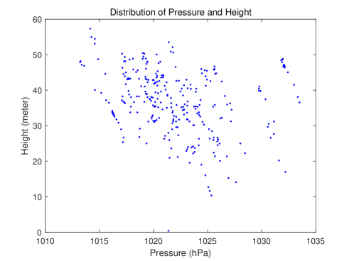
Figure 1: The distribution of the pressure values and the corresponding altitudes.

3.2 Outlier detection

In subsection 3.1, we have cleaned away the abnormal data which deviate too much from the dataset. However, there are still some outliers. An outlier is a point which differs significantly from the other points in a subdataset measured by the same device in a short time. We use the spherical distance computed by the haversine formula S1984 to identify the outlier. The haversine formula is illustrated by Fig. 2 and calculates the spherical distance between the two points $A(lon_{a},\,lat_{a})$ and $B(lon_{b},\,lat_{b})$ with the coordinate $(longitude,\,latitude)$ as follows:

$$d_{AD} =2Rsin(\Delta lon/2)cos(lat_{a}),$$

$$d_{CB} =2Rsin(\Delta lon/2)cos(lat_{b}),$$ (2)

$$d_{AB} =2R\left|sin^{2}\left(\frac{\Delta lat}{2}\right)+cos(lat_{a})cos(lat_{b})sin^{2}\left(\frac{\Delta lon}{2}\right)\right|^{\frac{1}{2}},$$

where $\Delta lon=lon_{b}-lon_{a}$, $\Delta lat=lat_{b}-lat_{a}$, and $R$ is the radius of the Earth.

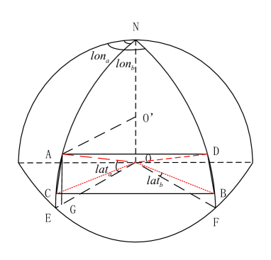
Figure 2: The diagram of two points in a three-dimensional space.

Consequently, we estimate the diameter of a subdataset as follows:

$$d_{max}=\bar{v}\times t,$$ (3)

where $\bar{v}$ is the mean velocity, and $t$ is the total measuring time of the subdataset. On the other hand, each point has a distance vector with other points. If over $50\%$ elements of the distance vector are greater than $d_{max}$, we regard this point as an outlier.

3.3 Data correction

In this subsection, we describe the procedure of data correction and it is also the key step of our positioning method. This step is to predict the relatively accurate altitudes of the outliers. As mentioned in section 3.2, the data distribution is roughly similar when the data are measured by the same device. Under this assumption, the altitudes of the subdataset are classified into different classes (labels). Thus, we encounter the multi-class classification problem.

3.3.1 The multi-class classification problem

The outliers of the subdataset have been found with the method in section 3.2. Thus, we select the data except outliers as a training dataset. The input training dataset is composed of $N$ pairwise points $(X_{n},\,h_{n})\,(n=1,\,2,\,\dots,N)$, where $X_{n}$ is the feature vector of the $n$-th point and $h_{n}$ is the corresponding altitude. Denote $h_{min}$ and $h_{max}$ as the minimum altitude and the maximum altitude, respectively. Parameter $\delta\,(h_{min}<\delta<h_{max}$) is the quantization step of altitude. Then, for a given altitude $h$, its corresponding class $k$ is computed as follows:

$$k=\left\lceil{\frac{h-h_{min}}{\delta}}\right\rceil+1,$$

where $h_{min}\leq h\leq h_{max}$,$\left\lceil{\cdot}\right\rceil$ is a function which will round the value toward positive infinity. When the predicted class of a point is obtained, we take the average altitude of its corresponding interval as the predicted altitude and which is computed by the following formula:

$$h^{p}_{k}=\left(k-\frac{1}{2}\right)\delta+h_{min},\;k=1,\,2,\,\ldots,\,K,$$ (4)

Thus, after the above transformation procedure, the data correction problem is converted into a multi-class classification problem (see Table 1, where $K$ represents the number of classes and $K=\lceil(h_{max}-h_{min})/\delta\rceil$+1).

Table 1: The class, its corresponding interval and predicted altitude.

Class	Interval (meter)	Predicted altitude (meter)
1	$h_{min}\sim\delta+h_{min}$	$\frac{1}{2}\delta+h_{min}$
2	$\delta+h_{min}\sim 2\delta+h_{min}$	$\frac{3}{2}\delta+h_{min}$
⋮	⋮	⋮
k	$(k-1)\delta+h_{min}\sim k\delta+h_{min}$	$\left(k-\frac{1}{2}\right)\delta+h_{min}$
⋮	⋮	⋮
K	$(K-1)\delta+h_{min}\sim K\delta+h_{min}$	$\left(K-\frac{1}{2}\right)\delta+h_{min}$

3.3.2 The weighted multinomial logistic regression model

Logistic Regression (LR) is a machine learning method and widely used to the binary classification problem C2006 . The MLR method extends the binary LR method to the multiple classification problem. For the MLR model, each class has its parameter vector. According to the parameter vector and the data feature vector, the MLR method determines the classification of the data. In the positioning application scenario, every feature vector consists of time, longitude, latitude, air pressure value and speed.

The training process of the MLR model needs to obtain the parameter $\omega_{k}$ of the $k$-th class via solving the the maximum likelihood function ZLC2012 , where $k=1,\,2,\,\cdots,K$. The conditional probability of the feature vector $X$ belonging to the class $Y$ is given by the following formula:

$$P(Y=k|X=x)=\frac{e^{\omega_{k}^{T}x}}{\sum^{K}_{i=1}e^{\omega_{i}^{T}x}},\;k=1,2,\cdots,K.$$ (5)

Then, the MLR method predicts the data category $k^{\ast}$ via solving the following maximum problem:

$$k^{\ast}\in\mathop{argmax}\limits_{k\in\{1,\,2,\,\ldots,\,K\}}P(Y=k|X=x).$$ (6)

After the data preprocessing of the previous steps, we obtain the training dataset, which consists of $N$ pairwise points $(X_{n},\,Y_{n})\,(n=1,\,2,\,\ldots,\,N)$, where $X_{n}$ represents the data feature vector and $Y_{n}$ represents its corresponding data class. According to formula (5) and the independent assumption of the multivariate distribution, we obtain the likelihood function as follows:

$$\prod^{N}_{n=1}P\left(Y=Y_{n}|X=X_{n}\right)=\prod^{N}_{n=1}\left(\frac{e^{\omega_{Y_{n}}^{T}X_{n}}}{\sum^{K}_{k=1}e^{\omega_{k}^{T}X_{n}}}\right).$$ (7)

Taking the logarithm of the two sides of formula (7), we obtain the following log-likelihood function:

$$log\left(\prod^{N}_{n=1}P\left(Y=Y_{n}|X=X_{n}\right)\right)=\sum^{N}_{n=1}\left(\omega_{Y_{n}}^{T}X_{n}-log\left({\sum^{K}_{k=1}e^{\omega_{k}^{T}X_{n}}}\right)\right).$$ (8)

Since the value of expression (8) is less than zero, we define function $f(\Omega)$ as

$$f(\Omega)=\sum^{N}_{n=1}\left(-\omega_{Y_{n}}^{T}X_{n}+log\left({\sum^{K}_{k=1}e^{\omega_{k}^{T}X_{n}}}\right)\right),$$ (9)

where $\Omega=[\omega_{1},\,\omega_{2},\,\ldots,\,\omega_{K}]$. Then, we obtain the maximum likelihood estimation $\Omega^{\ast}$ of parameter matrix $\Omega$ via solving the following optimization problem:

$$\Omega^{\ast}=\mathop{argmin}\limits_{\Omega}\ f(\Omega).$$ (10)

Since the training dataset is separable, the value of function $f(\Omega)$ can be made arbitrarily close to zero via multiplying $\Omega$ by a large value KS2016 . In order to maintain the finiteness of $\Omega$, we obtain the parameter matrix $\Omega^{\ast}$ by solving its regularized problem of problem (9) as follows:

$$\Omega^{*}=\mathop{argmin}\limits_{\Omega}\;\left(f(\Omega)+\lambda\eta(\Omega)\right),$$ (11)

where $\lambda>0$ is the regularized parameter and the regularized function $\eta(\Omega)$ is convex and non-smooth. For this convex optimization problem, there are many efficient optimization methods to tackle it such as the quasi-Newton BFGS method (p. 198, NW1999 ). Once the MLR model has been trained, we can predict the data category via solving the maximum problem (6).

We denote $\mathrm{I}=\{1,\,2,\,\ldots,\,I\}$ as the index set of the feature vector $X$, where $I$ represents the dimension of the feature vector $X$. Select randomly $r$ features from $I$ features and record the index of selected features as the subset $\mathrm{S}$ of the index set $\mathrm{I}$. Since the $\ell_{1}$ regularizer is easier to obtain a sparse solution than the $\ell_{2}$ regularizer, we define a group-$\ell_{1}$-regularizer as

$$\eta_{\mathrm{S}}(\Omega)=\sum_{i\in\mathrm{S}}\|[\Omega]_{\mathrm{I}_{i}}\|_{1},$$ (12)

where $[\Omega]_{\mathrm{I}_{i}}$ is the $\mathrm{I}_{i}$-th row of parameter matrix $\Omega$, and $\|x\|_{1}=\sum_{i=1}^{m}|x_{i}|\;\text{for vector}\;x\in\Re^{m}$. Thus, the problem (11) is written as the following group-sparse problem:

$$\min_{\Omega}\;\left(f(\Omega)+\lambda\eta_{\mathrm{S}}(\Omega)\right).$$ (13)

If the parameter $\lambda$ is suitably selected, the solution $\Omega^{\ast}$ of problem (13) will be group-row-sparse KCFH2005 .

After $L$ operations as the procedure above, we obtain $L$ parameter matrices $\Omega^{\ast}_{1}$,   $\Omega^{\ast}_{2},\,\ldots,\,\Omega^{\ast}_{L}$. Multiply the $L$ parameter matrices $\Omega^{\ast}_{l}\,(l=1,\,2,\,\ldots,L)$ by their corresponding sub-features, then we obtain the predicted categories $k_{l}^{\ast}\,(l=1,\,2,\,\ldots,\,L)$ with formulas (5)-(6) and its predicted altitudes $h_{l}^{p}\,(l=1,\,2,\,\ldots,L)$ with formula (4) as follows:

$$k^{\ast}_{l}=\mathop{argmax}\limits_{k\in\{1,\,2,\,\ldots,\,K\}}\left(\omega_{k}^{\ast l}\right)^{T}[X]_{\mathrm{S}_{l}},\;\text{and}\;h^{p}_{l}=\left(k^{\ast}_{l}-\frac{1}{2}\right)\delta+h_{min},\;l=1,\,2,\,\ldots,\,L,$$ (14)

where $[X]_{\mathrm{S}_{l}}$ represents the sub-features selected from the feature vector $X$ and the $i$-th element of $[X]_{\mathrm{S}_{l}}$ equals $X(\mathrm{S}_{l}(i))$, $\omega_{k}^{\ast l}$ is the $k$-th element of matrix $\Omega_{l}$.

Compute $L$ absolute errors between the original altitude $h$ and the $l$-th predicted altitude $h_{l}^{p}(l=1,\,2,\,\ldots,\,L)$ as follows:

$$Err_{l}=\left|h-h_{l}^{p}\right|,\;l=1,\,2,\,\ldots,L.$$ (15)

Then, we obtain the weighted predicted altitude of the feature vector as follows:

$$h^{\ast}=\sum^{L}_{l=1}w_{l}h_{l}^{p},$$ (16)

where the weighted coefficients $w_{l}\,(l=1,\,2,\,\ldots,\,L)$ are computed by the following formula:

$$w_{l}=\frac{Err_{l}}{\sum^{L}_{l=1}Err_{l}},\;l=1,\,2,\,\ldots,\,L.$$ (17)

According to the above discussions, we give the weighted multinomial logistic regression method for the vertical position problem in Algorithm 1.

Algorithm 1 The WMLR method for the vertical positioning problem

0:     the training data $(X_{n},h_{n}),n=1,\,2,\,\ldots,\,N$; the test feature vector $X$ and its corresponding altitude $h$.

0:     the predicted altitude $h^{\ast}$ of the feature vector $X$.

1:  Given the regularized parameter $\lambda$, the dimension $r$ of the sub-feature vector, the quantization step $\delta$ of altitude, the number of the group-sparse operations $L$.

2:  for $l=1,\,2,\,\ldots,\,L$ do

3:     Select randomly $r$ features from every feature vector of the training dataset and denote its corresponding index set of $r$ features as $\mathrm{S}_{l}$.

4:     Obtain the $l$-th regression coefficient matrix $\Omega^{\ast}_{l}$ via solving the optimization problem $\Omega_{l}^{\ast}=\mathop{argmin}\limits_{\Omega}\;\left(f(\Omega)+\lambda\eta_{\mathrm{S}_{l}}(\Omega)\right)$, where $f(\Omega)$ is defined by equation (11) and $\eta_{\mathrm{S}_{l}}(\Omega)$ is defined by equation (12).

5:     Obtain the predicted category $k^{\ast}_{l}$ and the $l$-th predicted altitude $h_{l}^{p}$ of the feature vector $X$ via solving problem (14).

6:     Compute the absolute error $Err_{l}$ between the original altitude and the predicted altitude of the feature vector $X$ from equation (15).

7:  end for

8:  Compute $L$ weighted coefficients $w_{l}\,(l=1,\,2,\,\ldots,\,L)$ from equation (17).

9:  Obtain the weighted predicted altitude $h^{\ast}$ of the feature vector $X$ from equation (16).

4 Numerical experiments

In this section, we compare the MLR method, the WMLR method (Algorithm 1) and the SVM method (coded by C. Chang and C. Lin, CL2013 ) for the vertical positioning problem. The programs are performed under the MATLAB environment MATLAB .

The raw dataset is provided by Huawei Technologies Company and collected by different user equipments. From Fig. 3, we find that there are 12796 UserIds and the number of data collected by each UserId is different. In the dataset, each piece of data includes time, longitude, latitude, speed, altitude and some data also contain barometric pressure value. The measurement time of the experiment dataset spans almost three months from October 5 to December 25, 2018. The air pressure is relatively high because the temperature is relatively low in that season. Except for null values, the data type is numeric.

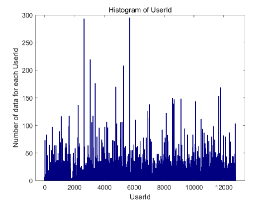
Figure 3: The data volume of the corresponding userID of the raw dataset

Since the raw dataset contains many null and abnormal values, we exclude those null and abnormal values with the method in subsection 3.1. Table 2 presents the statistical results of the cleaned data. From Table 2, we find that the distribution of data is not Gaussian. Thus, we standardize and normalize the data. After the data cleaning and normalization, we obtain a training set, every data element of which includes time, speed, longitude, latitude, pressure. We divide the dataset into two parts, i.e. $70\%$ data for training and $30\%$ data for testing.

Then, in order to verify the effect of Algorithm 1 (the WMLR method), we compare the performance of the MLR method, Algorithm 1, and the SVM method for the cleaned data. For Algorithm 1, we set the regularized parameter $\lambda=10^{-3}$, the quantization step $\delta=4$, the length of the group-sparse feature $r=4$ and $L=C_{5}^{4}=5$. The numerical results are put in Table 3 and Fig. 4. Table 3 is the statistical results of the vertical positioning accuracy predicted by three methods. From Table 3, we find that the vertical positioning accuracy is improved from 5.9 meters (the MLR method), 5.4 meters (the SVM method) to 5 meters (the WMLR method) for $67\%$ test points. Fig. 4 is the cumulative distribution function of the positioning accuracy. From Fig. 4, we find that the positioning error of WMLR is less than that of the SVM method and the WLR method when the cumulative probability is less than 90%, and the positioning accuracy of the SVM method is the best when the cumulative probability is greater than 90%.

Table 2: The statistical results of the cleaned data.

	longitude	latitude	speed	pressure	label	altitude
mean	121.5767	31.2595	5.8808	1021.3788	0.9181	22.9314
std	0.0030	0.0020	6.7051	1.2559	0.2742	10.9594
min	121.5708	31.2566	0.0000	1017.1787	0.0000	0.0534
25%	121.5742	31.2579	1.0000	1020.5680	1.0000	15.7657
50%	121.5765	31.2590	3.0000	1021.3281	1.0000	20.1303
75%	121.5792	31.2610	10.0000	1022.3744	1.0000	28.5893
max	121.5820	31.2653	26.0000	1024.0759	1.0000	78.1991

Table 3: Vertical positioning accuracies (m) of the MLR, WMLR and SVM methods.

	Min	Max	Mean	Median	Std	$67\%$	$90\%$
MLR	0.0211	48.8268	5.9795	4.4133	6.7941	5.9705	11.7054
WMLR	0.0211	31.9072	4.6628	3.2539	3.2539	5.0216	10.1085
SVM	0.0211	25.2855	4.9508	3.9297	4.0743	5.4383	10.3968

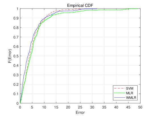
Figure 4: The comparison of three different methods.

5 Conclusion and future works

In this paper, a vertical positioning method with GPS information and the air pressure values is proposed. Firstly, we clean the missing and abnormal data. Then, according to the spherical distance matrix between points, we identify and exclude outliers. Consequently, we divide the cleaned data into two parts, i.e. $70\%$ data for training and $30\%$ data for testing. Based on the cleaned data, we compare the performances of the MLR method, the WMLR method (Algorithm 1), and the SVM method for this vertical positioning problem. The numerical results show that the vertical positioning accuracy is improved from 5.9 meters (the MLR method), 5.4 meters (the SVM method) to 5 meters (the WMLR method). Therefore, the WMLR method has some improvements of the positioning accuracy for this vertical positioning problem.

The appealing positioning technology based on the WMLR method is that this method does not rely on the empirical pressure-height formula and it can automatically adjust the parameter matrix according to the local area. The integration of the MLR method and the weighted technique considers all training points such that it smoothes the noise to get a better prediction. For the WMLR method, since it exists the quantization step, it will result in enlarging the positioning error when the point is the misclassification, which is a problem to be solved in the future work. Besides, due to the heterogeneity of user equipments and the complexity of the real environment, there are some room of improvement on the vertical positioning accuracy of the WMLR method.

Financial and Ethical Disclosures

• Funding: This work was supported in part by Grant 61876199 from National Natural Science Foundation of China, Grant YBWL2011085 from Huawei Technologies Co., Ltd., and Grant YJCB2011003HI from the Innovation Research Program of Huawei Technologies Co., Ltd..

• Conflict of Interest: The authors declare that they have no conflict of interest.

References

- (1) A. B. Adege, H. Lin, G. B. Tarekegn, Y. Y. Munaye and L. Yen, An indoor and outdoor positioning using a hybrid of support vector machine and deep neural network algorithms, Journal of Sensors, 2018, 1-12 (2018).
- (2) S. Alaee, A. Abdoli, C. Shelton, A. C. Murillo, A. C. Gerry and E. Keogh, Features or shape? Tackling the false dichotomy of time series classification, arXiv preprint, https://arxiv.org/abs/1912.09614, (2019).
- (3) N. Ali, B. Zafar, M. K. Iqbal, M. Sajid, M. Y. Younis, S. H. Dar, M. T. Mahmood and I. H. Lee, Modeling global geometric spatial information for rotation invariant classification of satellite images, PLoS ONE, 14 (7), 1-24 (2019).
- (4) S. Burgess, K. Åström, M. Högström and B. Lindquist, Smartphone positioning in multi-floor environments without calibration or added infrastructure, 2016 International Conference on Indoor Positioning and Indoor Navigation (IPIN), IEEE (2016).
- (5) C. Chang and C. Lin, Training -support vector classifiers: theory and algorithms, Neural Computation, 13, 2119-2147 (2001).
- (6) C. Chang and C. Lin, LIBSVM: a library for support vector machines, the software package available at https://www.csie.ntu.edu.tw/~cjlin/libsvm/, 2013.
- (7) B. Christopher M, Pattern Recognition and Machine Learning, Springer, New York, USA, 2006.
- (8) A. Chriki, H. Touati and H. Snoussi, SVM-based indoor localization in wireless sensor networks, 2017 13th International Wireless Communications and Mobile Computing Conference, 1144-1149 (2017).
- (9) H. Du, C. Zhang, Q. Ye, W. Xu, P. L. Kibenge and K. Yao, A hybrid outdoor localization scheme with high-position accuracy and low-power consumption, EURASIP Journal on Wireless Communications and Networking, 2018 (4), 1-13 (2018).
- (10) P. Gupta, S. Bharadwaj, S. Ramakrishnan and J. Balakrishnan, Robust floor determination for indoor positioning, 2014 Twentieth National Conference on Communications (NCC), Kanpur, 1-6 (2014).
- (11) T.-Y. He, X.-L. Luo and Z.-H. Liu, A probabilistic indoor localization algorithm based on restricted Boltzmann machine, Proceedings of 2017 IEEE 2nd Advanced Information Technology, Electronic and Automation Control Conference, 1364-1368 (2017).
- (12) J. Huang and C. Tsai, Improve GPS positioning accuracy with context awareness, 2008 First IEEE International Conference on Ubi-Media Computing, Lanzhou, 94-99 (2008).
- (13) M. Islam and J. Kim, An effective approach to improving low-cost GPS positioning accuracy in real-time navigation, The Scientific World Journal, 2014, 1-8 (2014), http://dx.doi.org/10.1155/2014/671494.
- (14) K. Kayabol, Approximate sparse multinomial logistic regression for classification, IEEE Transactions on Pattern Analysis and Machine Intelligence, 42 (2), 490-493 (2019).
- (15) T. Kim and S. Wright, PMU placement for line outage identification via multiclass logistic regression, IEEE Transactions on Smart Grid, 9 (1), 122-131 (2016).
- (16) B. Krishnapuram, L. Carin, M. A. T. Figueiredo and A. J. Hartemink, Sparse multinomial logistic regression: Fast algorithms and generalization bounds, IEEE Transactions on Pattern Analysis and Machine Intelligence, 27 (6), 957-968 (2005).
- (17) Z.-H. Liu, X.-L. Luo and T.-Y. He, Indoor positioning system based on the improved W-KNN algorithm, Proceedings of 2017 IEEE 2nd Advanced Information Technology, Electronic and Automation Control Conference, 1355-1359 (2017).
- (18) L. Meier, S. V. D. Geer and P. Bühlmann, The group Lasso for logistic regression, Journal of the Royal Statistical Society, 70 (1), 53-71 (2008).
- (19) MATLAB 9.6.0 (R2019a), The MathWorks Inc., http://www.mathworks.com, 2019.
- (20) J. Nocedal and S. J. Wright, Numerical Optimization, Springer-Verlag, 1999.
- (21) C. Ordóñez, J. R. Rodríguez-Pérez, J. J. Moreira, J. M. Matías and E. Sanz-Ablanedo, Machine learning techniques applied to the assessment of GPS accuracy under the forest canopy, Journal of Surveying Engineering, 137, 140-149 (2011).
- (22) M. Rohani, D. Gingras and D. Gruyer, A novel approach for improved vehicular positioning using cooperative map matching and dynamic base station DGPS concept, IEEE Transactions on Intelligent Transportation Systems, 17 (1), 230-239 (2015).
- (23) R. W. Sinnott, Virtues of the haversine, Sky and Telescope, 68 (2), 158-159 (1984).
- (24) Y. H. Wang, H. Li, X.-L. Luo, Q. M. Sun, J. N. Liu, A 3D fingerprinting positioning method based on cellular networks, International Journal of Distributed Sensor Networks, 1-9 (2014), http://dx.doi.org/10.1155/2014/248981.
- (25) P. Williams, Interactive Statistics for the Behavioral Sciences, Sinauer Associates, Inc. Publishers, Sunderland, Massachusetts USA, 2004.
- (26) H. Xia, X. Wang, Y. Qiao, J. Jian and Y. Chang, Using multiple barometers to detect the floor location of smart phones with built-in barometric sensors for indoor positioning, Sensors, 15(4), 7857-7877 (2015).
- (27) V. Zaliva and F. Franchetti, Barometric and GPS altitude sensor fusion, 2014 IEEE International Conference on Acoustics, Speech and Signal Processing, 1-5 (2014).
- (28) J. Zhu, X.-L. Luo and D. Chen, Maximum likelihood scheme for fingerprinting positioning in LTE system, 2012 IEEE 14th International Conference on Communication Technology, 428-432 (2012).
- (29) H. Zou, B. Huang, X. Lu, H. Jiang and L. Xie, A robust indoor positioning system based on the procrustes analysis and weighted extreme learning machine, IEEE Transactions on Wireless Communications, 15 (2), 1252-1266 (2016).