A fast methodology for large-scale focusing inversion of gravity and magnetic data using the structured model matrix and the $2D$ fast Fourier transform

Abstract.

Focusing inversion of potential field data for the recovery of sparse subsurface structures from surface measurement data on a uniform grid is discussed. For the uniform grid the model sensitivity matrices exhibit block Toeplitz Toeplitz block structure, by blocks for each depth layer of the subsurface. Then, through embedding in circulant matrices, all forward operations with the sensitivity matrix, or its transpose, are realized using the fast two dimensional Fourier transform. Simulations demonstrate that this fast inversion algorithm can be implemented on standard desktop computers with sufficient memory for storage of volumes up to size $n\approx 1M$. The linear systems of equations arising in the focusing inversion algorithm are solved using either Golub-Kahan-bidiagonalization or randomized singular value decomposition algorithms in which all matrix operations with the sensitivity matrix are implemented using the fast Fourier transform. These two algorithms are contrasted for efficiency for large-scale problems with respect to the sizes of the projected subspaces adopted for the solutions of the linear systems. The presented results confirm earlier studies that the randomized algorithms are to be preferred for the inversion of gravity data, and that it is sufficient to use projected spaces of size approximately $m/8$, for data sets of size $m$. In contrast, the Golub-Kahan-bidiagonalization leads to more efficient implementations for the inversion of magnetic data sets, and it is again sufficient to use projected spaces of size approximately $m/8$. Moreover, it is sufficient to use projected spaces of size $m/20$ when $m$ is large, $m\approx 50000$, to reconstruct volumes with $n\approx 1M$. Simulations support the presented conclusions and are verified on the inversion of a practical magnetic data set that is obtained over the Wuskwatim Lake region in Manitoba, Canada.

Rosemary A. Renaut

School of Mathematical and Statistical Sciences

Arizona State University

Tempe, AZ 85287, USA

Jarom D. Hogue

School of Mathematical and Statistical Sciences, Arizona State University

Tempe, AZ 85287, USA

Saeed Vatankhah

Institute of Geophysics, University of Tehran, Tehran, Iran

Hubei Subsurface Multi-scale Imaging Key Laboratory, Institute of Geophysics and Geomatics

China University of Geosciences, Wuhan, China.

1. Introduction

The determination of the subsurface structures from measured potential field data is important for many practical applications concerned with oil and gas exploration, mining, and regional investigations, Blakely [1995]; Nabighian et al. [2005]. There are many approaches that can be considered for the inversion of potential field data sets. These range from techniques that directly use the inversion of a forward model described by a sensitivity matrix for gravity and magnetic potential field data, as in, for example, Boulanger and Chouteau [2001]; Farquharson [2008]; Lelièvre and Oldenburg [2006]; Li and Oldenburg [1996, 1998]; Pilkington [1997]; Silva and Barbosa [2006] and Portniaguine and Zhdanov [1999]. Other approaches avoid the problem with the storage and generation of a large sensitivity matrix by employing alternative approaches, as in Cox et al. [2010]; Uieda and Barbosa [2012]; Vatankhah et al. [2019]. Of those that do handle the sensitivity matrix, some techniques to avoid the large scale challenge, include wavelet and compression techniques, Li and Oldenburg [2003]; Portniaguine and Zhdanov [2002] and Voronin et al. [2015]. Of interest here is the development of an approach that takes advantage of the structure that can be realized for the sensitivity matrix, and then enables the use of the fast Fourier transform for fast matrix operations, and avoids the high storage overhead of the matrix.

The efficient inversion of three dimensional gravity data using the $2$D fast Fourier transform (2DFFT) was presented in the Master’s thesis of [Bruun and Nielsen, 2007]. There, it was observed that the sensitivity matrix exhibits a block Toeplitz Toeplitz block (BTTB) structure provided that the data measurement positions are uniform and carefully related to the grid defining the volume discretization. It is this structure which facilitates the use of the 2DFFT via the embedding of the required kernel entries that define the sensitivity matrix within a block Circulant Circulant block (BCCB) matrix, and which is explained in Chan and Jin [2007]; Vogel [2002]. Then, Zhang and Wong [2015] used the BTTB structure for fast computations with the sensitivity matrix, and employed this within an algorithm for the inversion of gravity data using a smoothing regularization, allowing for variable heights of the individual depth layers in the domain. They also applied optimal preconditioning for the BTTB matrices using the approach of Chan and Jin [2007]. Their approach was then optimized by Chen and Liu [2018] but only for efficient forward gravity modeling and with a slight modification in the way that the matrices for each depth layer of the domain are defined using the approximation of the forward integral equation. In particular, Zhang and Wong [2015] use a multilayer approximation of the gravity kernel, rather than the derivation of the kernel integral in Li and Chouteau [1998]. They noted, however, that their approach is subject to greater potential for error on coarse-grained domains because it does not use the exact kernel integral developed by Li and Chouteau [1998]. Bruun and Nielsen [2007] also developed an algorithm that is even more efficient in memory and computation than the use of the BTTB for each depth layer by using an upward continuation method to deal with the issue that measured data are only provided at the surface of the domain. They concluded that this was not suitable for practical problems. Finally, they also considered the interpolation of data not on the uniform grid to the uniform grid, hence removing the restriction on the uniform placement of measurement stations on the surface, but potentially introducing some error due to the interpolation. On the other hand, their study did not include Tikhonov stabilization for the solution of the linear systems, and hence did not implement state-of-the-art approaches for resolving complex structures with general L_p norm regularizers ($0\leq p\leq 2$). Moreover, standard techniques for inclusion of depth weighting, and imposition of constraint conditions were not considered. The focus of this work is, therefore, a demonstration and validation of efficient solvers that are more general and can be effectively employed for the independent focusing inversion of both large scale gravity and magnetic potential field data sets. It should be noted, moreover, that the approach can be applied also for domains with padding, which is of potential benefit for structure identification near the boundaries of the analyzed volume.

First, we note that the fast computation of geophysics kernel models using the fast Fourier transform (FFT) has already been considered in a number of different contexts. These include calculation using the Fourier domain as in Li et al. [2018]; Zhao et al. [2018], and also by Pilkington [1997] in conjunction with the conjugate gradient method for solving the magnetic susceptibility inverse problem. Fast forward modeling of the magnetic kernel on an undulated surface, combined with spline interpolation of the surface data was also suggested by Li et al. [2018] using an implementation of the model in the wave number domain. Further, fast forward and high accuracy modeling of the gravity kernel using the Gauss 2DFFT was discussed by Zhao et al. [2018]. Moreover, the derivation of the forward modeling operators that yield the BTTB structure for the magnetic and gravity kernels in combination with domain padding and the staggered placement of measurement stations with respect to the domain prisms at the surface was carefully presented in Hogue et al. [2019]. Hence, here, we only present necessary details concerning the development of the forward modeling approach

Associated with the development of a focusing inversion algorithm, is the choice of solver within the inversion algorithm, the choice of regularizer for focusing the subsurface structures, and a decision on determination of suitable regularization parameters. With respect to the solver, small scale problems can be solved using the full singular value decomposition (SVD) of the sensitivity matrix, which is not feasible for the large scale. Moreover, the use of the SVD for focusing inversion has been well-investigated in the literature, see for example [Vatankhah et al., 2014, 2015], while choices and implementation details for focusing inversion are reviewed in [Vatankhah et al., 2020b]. Furthermore, methods that yield useful approximations of the SVD, hence enabling automatic but efficient techniques for choice of the regularization parameters have also been discussed in [Renaut et al., 2017; Vatankhah et al., 2017] when considered with iterative Krylov methods based on the Golub-Kahan Bidiagonalization (GKB) algorithm, [Paige and Saunders, 1982], and in Vatankhah et al. [2018, 2020a] when adopted using the randomized singular value decomposition (RSVD), [Halko et al., 2011]. Recommendations for the application of the RSVD with power iteration, and the sizes of the projected spaces to be used for both GKB and RSVD were presented, but only within the context of problems that can be solved without the use of the 2DFFT. Thus, a complete validation of these algorithms for the solution of the large scale focusing inversion problem, with considerations contrasting the effectiveness of these algorithms in the large scale, is still important, and is addressed here.

We comment, further, that there is an alternative approach for the comparison of RSVD and GKB algorithms, which was discussed by Luiken and van Leeuwen [2020]. The focus there, on the other hand, was on the effective determination of both the size of the projected space and the determination of the optimal regularization parameter, using these algorithms. Their RSVD algorithm used the range finder suggested in [Halko et al., 2011, Algorithm 4], rather than the power iteration. They concluded with their one rather small example for an under-determined sensitivity matrix of size $400$ by $2500$ that this was not successful. The test for the GKB approach was successful for this problem, but it is still rather small scale as compared to the problems considered here. Instead as stated, we return to the problem of assessing a suitable size of the projected space to be used for large scale inversion of magnetic and gravity data, using the techniques that provide an approximate SVD and hence efficient and automatic estimation of the regularization parameter concurrently with solving large scale problems. We use the method of Unbiased Predictive Risk Estimation (UPRE) for automatically estimating the regularization parameters, as extensively discussed elsewhere, Vogel [2002].

Overview of main scientific contributions. This work provides a comprehensive study of the application of the 2DFFT in focusing inversion algorithms for gravity and magnetic potential field data sets. Specifically, our main contributions are as follows. (i) A detailed review of the mechanics for the inversion of potential field data using focusing inversion algorithms based on the iteratively regularized least squares algorithm in conjunction with the solution of linear systems using GKB or RSVD algorithms; (ii) The extension of these approaches for the use of the 2DFFT for all forward multiplications with the sensitivity matrix, or its transpose; (iii) Comparison of the computational cost when using the 2DFFT as compared to the sensitivity matrix, or its transpose, directly, when implemented within the inversion algorithm, and dependent on the sizes of the projected spaces adopted for the inversion; (iv) Presentation of numerical experiments that confirm that the RSVD algorithm is more efficient than the GKB for the inversion of gravity data sets, for larger problems than previously considered; (v) A new comparison the use of GKB as compared for RSVD for the inversion of magnetic data sets, showing that GKB is to be preferred; (vi) Finally, all conclusions are confirmed by application on a practical data set, demonstrating that the methodology is suitable for focusing inversion of large scale data sets and can provide parameter reconstructions with more than $1$M variables using a laptop computer.

The paper is organized as follows. In Section 2 we present the general methodology used for the independent inversion of gravity and magnetic potential field data. The BTTB details are reviewed in Section 2.1 and stabilized inversion is reviewed in Section 2.2. Details for the numerical solution of the inversion formulation are provided in Section 2.3 and the algorithms are in Section 2.4. The estimated computational cost of each algorithm, in terms of the number of floating point operations flops is given in Section 2.5. Numerical results applying the presented algorithms to synthetic and practical data are described in Section 3, with the details that apply to all computational implementations given in Section 3.1 and the generation of the synthetic data used in the simulations provided in Section 3.2. Results assessing comparison of computational costs for one iteration of the algorithm for use with, and without, the 2DFFT are discussed in Section 3.3.1. The convergence of the 2DFFT-based algorithms for problems of increasing size is discussed in Section 3.3.2. Validating results for the inversion of real magnetic data obtained over a portion of the Wuskwatim Lake region in Manitoba, Canada are provided in Section 3.4 and conclusions in Section 4. A provides brief details on the implementation of the computations using the embedding of the BTTB matrix in the BCCB matrix and the 2DFFT, and supporting numerical evidence of the figures illustrating the results are provided in a number of tables in B.

2. Methodology

2.1. Forward Model and BTTB Structure

We consider the inversion of measured potential field data $\mathbf{d}_{\mathrm{obs}}$ that describes the response at the surface due to unknown subsurface model parameters $\mathbf{m}$. The data and model parameters are connected via the forward model

(1) $$\mathbf{d}_{\mathrm{obs}}=G\mathbf{m},$$

where $G$ is the sensitivity, or model, matrix. This linear relationship is obtained via the discretization of a Fredholm integral equation of the first kind,

(2) $$d(a,b,c)=\int\int\int h(a,b,c,x,y,z)\zeta(x,y,z)dx\,dy\,dz,$$

where exact values $\mathbf{d}$ and $\mathbf{m}$ are the discretizations of continuous functions $d$ and $\zeta$, respectively, and $G$ in (1) provides the discrete approximation of the integrals of the kernel function $h$ over the volume cells. For the specific kernels associated with gravity and magnetic data, assuming for magnetic data that there is no remanence magnetization or self-magnetization, $h$ is spatially invariant in all dimensions, $h(a,b,c,x,y,z)=h(x-a,y-b,z-c)$ and (2) describes a convolution operation.

Using the formulation of the integral of the kernel as derived by Haáz [1953]; Li and Chouteau [1998] for the gravity kernel, and by Rao and Babu [1991] for the magnetic kernel, sensitivity matrix $G$ decomposes by column blocks as

(3) $$G=[G^{(1)},\dots,G^{(n_{z})}],$$

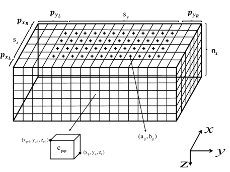
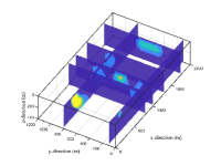
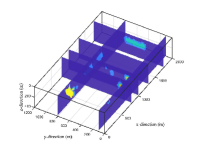
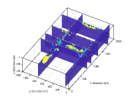
where block $G^{(r)}$ is for the $r^{\mathrm{th}}$ depth layer. The individual entries in $G$ correspond to the projections of the contributions from prisms $c_{pqr}$ in the volume to measurement stations, denoted by $s_{ij}$, at or near the surface. The configurations of the volume and measurement domains are illustrated in Figure 1. Here it is assumed that the measurement stations are all on the surface with coordinates $(a_{i},b_{j},0)$ in $(x,y,z)$. Prism $c_{pqr}$ of the domain has dimensions $\Delta_{x}$, $\Delta_{y}$ and $\Delta_{z}$ in $x$, $y$ and $z$ directions with coordinates that are integer multiples of $\Delta_{x}$, $\Delta_{y}$ and $\Delta_{z}$, and is indexed by $1\leq p\leq s_{x}+p_{x_{\texttt{L}}}+p_{x_{\texttt{R}}}=n_{x}$, $1\leq q\leq s_{y}+p_{y_{\texttt{L}}}+p_{y_{\texttt{R}}}=n_{y}$, and $1\leq r\leq n_{z}$. This indexing assumes that there is padding around the domain in $x$ and $y$ directions by additional borders of $p_{x_{\texttt{L}}}$, $p_{x_{\texttt{R}}}$, $p_{y_{\texttt{L}}}$ and $p_{y_{\texttt{R}}}$ cells. The distinction between the padded and unpadded portions of the domain is that there are no measurement stations in the padded regions. This yields $G\in\mathcal{R}^{m\times n}$ where $m=s_{x}s_{y}$, and $n=n_{x}n_{y}n_{z}$, and each $G^{(r)}\in\mathcal{R}^{m\times n_{r}}$, where $n_{r}=n_{x}n_{y}$.

Figure 1. The configuration of prism $c_{pqr}$, $1\leq p\leq s_{x}+p_{x_{\texttt{L}}}+p_{x_{\texttt{R}}}=n_{x}$, $1\leq q\leq s_{y}+p_{y_{\texttt{L}}}+p_{y_{\texttt{R}}}=n_{y}$, $1\leq r\leq n_{z}$, in the volume relative to a station on the surface at location $s_{ij}=(a_{ij},b_{ij})$, $1\leq i\leq s_{x}$, $1\leq j\leq s_{y}$. Here the stations are shown as located at the centers of the cells on the surface of the domain and that there are no measurements taken in the padded portion of the domain.

In (3), $m\leq n_{r}\ll n$ and the system is drastically underdetermined for any reasonable discretization of the depth ($z$) dimension of the volume. Moreover, when $n$ is large the use of the matrix $G$ requires both significant computational cost for evaluation of matrix-matrix operations and significant storage. Without taking account of structure in $G$, and assuming that a dot product of real vectors of length $n$ requires $2n$ floating point operations (flops), calculating $GH$, for $H\in\mathcal{R}^{n\times p}$, takes $\mathcal{O}(2nmp)$ flops and storage of matrix $G$ uses approximately $8mn\times 1e^{-9}$GB. For example, suppose $p=m=n/8$ and $n=10^{6}$, then storage of $G$ requires approximately $1000$GB, and the single matrix multiplication uses $\approx 10^{18}/32~{}\texttt{flops}$ or $10^{7}\mathrm{G}\texttt{flops}$, without any consideration of additional software and system overheads. These observations limit the ability to do large scale stabilized inversion of potential field data in real time using current desktop computers, or laptops, without taking into account any further information on the structure of $G$. This is the topic of the further discussion here.

Bruun and Nielsen [2007] observed that the configuration of the locations of the stations in relation to the domain discretization is significant in generating $G^{(r)}$ with structure that can be effectively utilized to improve the efficiency of operations with $G$ and to reduce the storage requirements. Assuming that the stations are always placed uniformly with respect to the domain prisms, and provided that the distances between stations are fixed in $x$ and $y$, then matrix $G^{(r)}$ for the gravity kernel has symmetric BTTB structure (SBTTB). Then, it is possible to embed $G^{(r)}$ in a BCCB matrix and matrix operations can be efficiently performed using the 2DFFT, as explained in [Vogel, 2002]. This structure was also discussed and then utilized for efficient forward operations with $G$ in Chen and Liu [2018]. There it was assumed that the stations are placed symmetrically with respect to the domain coordinates, as illustrated for the staggered configuration in Figure 1 with the stations at the center of the cells on the surface. With respect to the magnetic kernel, Bruun and Nielsen [2007] demonstrated $G^{(r)}$ can also exhibit BTTB structure, but they did not use the standard computation of the magnetic kernel integral as described in Rao and Babu [1991]. On the other hand, a thorough derivation of the BTTB structure for $G^{(r)}$ using the approach of Rao and Babu [1991] has been given in Hogue et al. [2019]. That analysis also considered for the first time the use of the padding for the domain and the modifications required in the generation of the required entries in the matrix $G^{(r)}$. It should be noted, as shown in Hogue et al. [2019], that regardless of whether operations with $G$ are implemented using the 2DFFT or by direct multiplication, it is far faster to generate $G$ taking advantage of the BTTB structure. Here, we are concerned with efficient stabilized inversion of potential field data using this BTTB structure, and thus refer to A for a brief discussion of the implementation of the needed operations using $G$ when implemented using the 2DFFT, and point to Hogue et al. [2019] for the details.

2.2. Stabilized Inversion

The solution of (1) is an ill-posed problem; even if $G$ is well-conditioned the problem is underdetermined because $m\ll n$. There is a considerable literature on the solution of this ill-posed problem and we refer in particular to Vatankhah et al. [2020b] for a relevant overview, and specifically the use of the unifying framework for determining an acceptable solution of (1) by stabilization. Briefly, here we estimate $\mathbf{m}^{*}$ as the minimizer of the nonlinear objective function $\Phi_{\mathrm{\alpha}}(\mathbf{m})$ subject to bound constraints $\mathbf{m}_{\mathrm{min}}\leq\mathbf{m}\leq\mathbf{m}_{\mathrm{max}}$

(4) $$\mathbf{m}^{*}=\underset{\mathbf{m}_{\mathrm{min}}\leq\mathbf{m}\leq\mathbf{m}_{\mathrm{max}}}{\arg\min}\,\{\Phi_{\mathrm{\alpha}}(\mathbf{m})\}=\underset{\mathbf{m}_{\mathrm{min}}\leq\mathbf{m}\leq\mathbf{m}_{\mathrm{max}}}{\arg\min}\,\{\Phi_{\mathrm{d}}(\mathbf{m})+\alpha^{2}\Phi_{\mathrm{S}}(\mathbf{m})\}.$$

Here $\alpha$ is a regularization parameter which trades off the relative weighting of the two terms $\Phi_{\mathrm{d}}(\mathbf{m})$ and $\Phi_{\mathrm{S}}(\mathbf{m})$, which are respectively the weighted data misfit and stabilizer, given by

(5) $$\Phi_{\mathrm{d}}(\mathbf{m})=\|\mathbf{W_{\mathbf{d}}}(G\mathbf{m}-\mathbf{d}_{\mathrm{obs}})\|_{2}^{2},\text{ and }\Phi_{\mathrm{S}}(\mathbf{m})=\|\mathbf{W_{\mathrm{h}}}\mathbf{W_{\mathrm{z}}}\mathbf{W_{{\mathrm{L}}}}D(\mathbf{m}-\mathbf{m}_{\mathrm{apr}})\|_{2}^{2}.$$

The weighting matrices $\mathbf{W_{\mathbf{d}}}$, $\mathbf{W_{\mathrm{h}}}$, $\mathbf{W_{\mathrm{z}}}$ and $\mathbf{W_{{\mathrm{L}}}}$ are all diagonal, with dimensions that depend on the size of $D$, which can be used to yield an approximation for a derivative. Here, while we assume throughout that $D=I_{n\times n}$ and refer to [Vatankhah et al., 2020b, Eq. (5)] for the modification in the weighting matrices that is required for derivative approximations using $D$, we present this general formulation in order to place the work in context of generalized Tikhonov inversion. We also use $\mathbf{m}_{\mathrm{apr}}=\mathbf{0}$, but when initial estimates for the parameter are available, perhaps from physical measurements, note that these can be incorporated into $\mathbf{m}_{\mathrm{apr}}$ as an initial estimate for $\mathbf{m}$. The weighting matrix $\mathbf{W_{\mathbf{d}}}$ has entries $(\mathbf{W_{\mathbf{d}}})_{ii}=1/\sigma_{i}$ where we suppose that the measured data can be given by $\mathbf{d}_{\mathrm{obs}}=\mathbf{d}_{\mathrm{exact}}+\bm{\eta}$, where $\mathbf{d}_{\mathrm{exact}}$ is the exact but unknown data, and $\bm{\eta}$ is a noise vector drawn from uncorrelated Gaussian data with variance components $\sigma_{i}^{2}$.

Whereas stabilizer matrix $\mathbf{W_{{\mathrm{L}}}}$ in $\mathbf{W}=\mathbf{W_{\mathrm{h}}}\mathbf{W_{\mathrm{z}}}\mathbf{W_{{\mathrm{L}}}}$ depends on $\mathbf{m}$, $\mathbf{W_{\mathrm{h}}}$ and $\mathbf{W_{\mathrm{z}}}$ are constant hard constraint and constant depth weighting matrices. Although $\mathbf{W_{\mathrm{h}}}$ can be used to impose specific known values for entries of $\mathbf{m}$, as discussed in [Boulanger and Chouteau, 2001], we will use $\mathbf{W_{\mathrm{h}}}=I_{n\times n}$. Depth weighting $\mathbf{W_{\mathrm{z}}}$ is routinely used in the context of potential field inversion and is imposed to counteract the natural decay of the kernel with depth. With the same column structure as for $G$, $\mathbf{W_{\mathrm{z}}}=\texttt{blockdiag}(\mathbf{W_{\mathrm{z}}}^{(1)},\dots,\mathbf{W_{\mathrm{z}}}^{(n_{z})})$ where $\mathbf{W_{\mathrm{z}}}^{(r)}=(.5(z_{r}+z_{r-1}))^{-\beta}I_{n_{r}\times n_{r}}$, $.5(z_{r}+z_{r-1})$ is the average depth for depth level $r$, and $\beta$ is a parameter that depends on the data set, [Li and Oldenburg, 1996]. Now, diagonal matrix $\mathbf{W_{{\mathrm{L}}}}$ depends on the parameter vector $\mathbf{m}$ via $i^{\mathrm{th}}$ entry given by

(6) $$(\mathbf{W_{{\mathrm{L}}}})_{ii}=\left((\mathbf{m}_{i}-(\mathbf{m}_{\mathrm{apr}})_{i})^{2}+\epsilon^{2}\right)^{\frac{\lambda-2}{4}},\quad i=1\dots n,$$

where parameter $\lambda$ determines the form of the stabilization, and focusing parameter $0<\epsilon\ll 1$ is chosen to avoid division by zero. We use $\lambda=1$ which yields an approximation to the $L_{1}$ norm as described in [Wohlberg and Rodríguez, 2007], and is preferred for inversion of potential field data, although we note that the implementation makes it easy to switch to $\lambda=0$, yielding a solution which is compact, or $\lambda=2$ for a smooth solution. Based on prior studies we use $\epsilon^{2}=1e-9$, [Vatankhah et al., 2017].

2.3. Numerical Solution

We first reiterate that (4) is only nonlinear in $\mathbf{m}$ through the definition of $\mathbf{W_{{\mathrm{L}}}}$. Supposing that $\mathbf{W_{{\mathrm{L}}}}$ is constant and that $\mathrm{null}(\mathbf{W_{\mathbf{d}}}G)\cap\mathrm{null}(\mathbf{W})=\emptyset$, then the solution $\mathbf{m}^{*}$ of (4) without the bound constraints is given analytically by

(7) $$\mathbf{m}=\mathbf{m}_{\mathrm{apr}}+(G^{T}\mathbf{W_{\mathbf{d}}}^{T}\mathbf{W_{\mathbf{d}}}G+\alpha^{2}\mathbf{W}^{T}\mathbf{W})^{-1}G^{T}\mathbf{W_{\mathbf{d}}}^{T}\mathbf{W_{\mathbf{d}}}(\mathbf{d}_{\mathrm{obs}}-G\mathbf{m}_{\mathrm{apr}}).$$

Equivalently, assuming that $\mathbf{W}$ is invertible, and defining $\tilde{G}=\mathbf{W_{\mathbf{d}}}G\mathbf{W}^{-1}$, $\tilde{\mathbf{r}}=\mathbf{W_{\mathbf{d}}}(\mathbf{d}_{\mathrm{obs}}-G\mathbf{m}_{\mathrm{apr}})$ and $\mathbf{y}=\mathbf{m}-\mathbf{m}_{\mathrm{apr}}$, then $\mathbf{y}$ solves the normal equations

(8) $$\mathbf{y}=\mathbf{W}^{-1}(\tilde{G}^{T}\tilde{G}+\alpha^{2}I)^{-1}\tilde{G}^{T}\tilde{\mathbf{r}},$$

and $\mathbf{m}^{*}$ can be found by restricting $\mathbf{y}+\mathbf{m}_{\mathrm{apr}}$ to lie within the bound constraints.

Now (8) can be used to obtain the iterative solution for (4) using the iteratively reweighted least squares (IRLS) as described in Vatankhah et al. [2020b]. Specifically, we use superscript $k$ to indicate a variable at an iteration $k$, and replace $\alpha$ by $\alpha^{(k)}$, $\mathbf{W_{{\mathrm{L}}}}$ by matrix $\mathbf{W}^{(k)}_{{\mathrm{L}}}$ with entries $(\mathbf{W}^{(k)}_{{\mathrm{L}}})_{ii}=\left((\mathbf{m}^{(k-1)}_{i}-\mathbf{m}^{(k-2)}_{i})^{2}+\epsilon^{2}\right)^{\frac{\lambda-2}{4}}$ and $\mathbf{m}-\mathbf{m}_{\mathrm{apr}}$ by $\mathbf{m}-\mathbf{m}^{(k-1)}$, initialized with $\mathbf{W_{{\mathrm{L}}}}^{(1)}=I$, and $\mathbf{m}^{(0)}=\mathbf{m}_{\mathrm{apr}}$ respectively. Then $\mathbf{y}^{(k)}$ is found as the solution of the normal equations (8), and $\mathbf{m}^{(k)}$ is the restriction of $\mathbf{y}^{(k)}+\mathbf{m}^{(k-1)}$ to the bound constraints.

This use of the IRLS algorithm for the incorporation of the stabilization term $\Phi_{\mathrm{S}}$ contrasts the implementation discussed in [Zhang and Wong, 2015] for the inversion of potential field gravity data. In their presentation, they considered the solution of the general smoothing Tikhonov formulation described by (8) for general fixed smoothing operator $D$ replacing $\mathbf{W_{{\mathrm{L}}}}$. For the solver, they used the re-weighted regularized conjugate solver for iterations to improve $\mathbf{m}^{(k)}$ from $\mathbf{m}_{\mathrm{apr}}$. They also included a penalty function to impose positivity in $\mathbf{m}^{(k)}$, depth weighting to prevent the accumulation of the solution at the surface, and adjustment of $\alpha$ with iteration $k$ to encourage decrease in the data fit term. Moreover, they showed that it is possible to pick approximations $D$ which also exhibit BTTB structure for each depth layer, so that $D\mathbf{x}$ can also be implemented by layer using the 2DFFT. Although we do not consider the unifying stabilization framework here with general operator $D$ as described in Vatankhah et al. [2020b], it is a topic for future study, and a further extension of the work, therefore, of Zhang and Wong [2015] for the more general stabilizers. In the earlier work of the use of the BTTB structure arising in potential field inversion, Bruun and Nielsen [2007] investigated the use of a truncated SVD and the conjugate gradient least squares method for the minimization of the data fit term without regularization. They also considered the direct solution of the constant Tikhonov function with $\mathbf{W_{{\mathrm{L}}}}=I$ and a fixed regularization parameter $\alpha$, for which the solution uses the filtered SVD in the small scale. Here, not only do we use the unifying stabilization framework, but we also estimate $\alpha$ at each iteration of the IRLS algorithm. The IRLS algorithm is implemented with two different solvers that yield effective approximations of a truncated SVD. One is based on the randomized singular value decomposition (RSVD), and the second uses the Golub Kahan Bidiagonalization (GKB).

2.4. Algorithmic Details

The IRLS algorithm relies on the use of an appropriate solver for finding $\mathbf{y}^{(k)}$ as the solution of the normal equations (8) for each update $k$, and a method for estimating the regularization parameter $\alpha^{(k)}$. While any suitable computational scheme can be used to update $\mathbf{m}^{(k)}$, the determination of $\alpha^{(k)}$ automatically can be challenging. But if the solution technique generates the SVD for $\tilde{G}^{(k)}$, or an approximation to the SVD, such as by use of the RSVD or GKB factorization for $\tilde{G}^{(k)}$, then there are many efficient techniques that can be used such as the unbiased predictive risk estimator (UPRE) or generalized cross validation (GCV). The obtained estimate for $\alpha^{(k)}$ depends on the estimator used and there is extensive literature on the subject, e.g. Hansen [2010]. Thus, here, consistent with earlier studies on the use of the GKB and RSVD for stabilized inversion, we use the UPRE, denoted by $U(\alpha)$, for all iterations $k>1$, and refer to Renaut et al. [2017] and Vatankhah et al. [2018, 2020a] for the details on the UPRE. The GKB and RSVD algorithms play, however, a larger role in the discussion and thus for clarity are given here as Algorithms 1 and 2, respectively.

For the use of the GKB we note that Algorithm 1 uses the factorization $\tilde{G}A_{t_{p}}=H_{t_{p}+1}B_{t_{p}}$, where $A_{t_{p}}\in\mathcal{R}^{n\times t_{p}}$ and $H_{t_{p}+1}\in\mathcal{R}^{m\times t_{p}+1}$. Steps 1 and 1 of Algorithm 1 apply the modified Gram-Schmidt re-orthogonalization to the columns of $A_{t_{p}}$ and $H_{t_{p}+1}$, as is required to avoid the loss of column orthogonality. This factorization is then used in Step 1 to obtain the rank $t_{p}$ approximate SVD given by $\tilde{G}=(H_{t_{p}+1}U_{t_{p}})\Sigma_{t_{p}}(A_{t_{p}}V_{t_{p}})^{T}$. The quality of this approximation depends on the conditioning of $\tilde{G}$, [Paige and Saunders, 1982]. In particular, the projected system of the GKB algorithm inherits the ill-conditioning of the original system, rather than just the dominant terms of the full SVD expansion. Thus, the approximate singular values include dominant terms that are good approximations to the dominant singular values of the original system, as well as very small singular values that approximate the tail of the singular spectrum of the original system. The accuracy of the dominant terms increases quickly with increasing $t_{p}$, Paige and Saunders [1982]. Therefore, to effectively regularize the dominant spectral terms from the rank $t_{p}$ approximation, in Step 1 we use the truncated UPRE that was discussed and introduced in Vatankhah et al. [2017]. Specifically, a suitable choice for $\alpha^{(k)}$ is found using the truncated SVD of $B_{t_{p}}$ with $t$ terms. Then, in Step 1, $\mathbf{y}^{(k)}$ is found using all terms in the expansion of $B_{t_{p}}$. The matrix $\Gamma(\alpha,\Sigma)$ in Step 1 is the diagonal matrix with entries $\sigma_{i}/(\sigma_{i}^{2}+\alpha^{2})$. In our simulations we use $t_{p}=\texttt{floor}(1.05\,t)$ corresponding to $5\%$ increase in the space obtained. This contrasts to using just $t$ terms and will include terms from the tail of the spectrum. Note, furthermore, that the top $t$ terms, from the projected space of size $t_{p}>t$ will be more accurate estimates of the true dominant $t$ terms than if obtained with $t_{p}=t$. Effectively, by using a $5\%$ increase of $t$ in the calculation of $t_{p}$, we assume that the first $t$ terms from the $t_{p}$ approximation provide good approximations of the dominant $t$ spectral components of the original matrix $\tilde{G}$. We reiterate that the presented algorithm depends on parameters $t_{p}$ and $t$. At Step 1 in Algorithm 1 $\alpha^{(k)}$ is found using the projected space of size $t$ but the update for $\mathbf{y}$ in Step 1 uses the oversampled projected space of size $t_{p}$. The results presented for the synthetic tests will demonstrate that this uniform choice for $t_{p}$ is a suitable compromise between taking $t_{p}$ too small and contaminating the solutions by components from the less accurate approximations of the small components, and a reliable, but larger, choice for $t_{p}$ that provides a good approximation of the dominant terms within reasonable computational cost.

Input: $\tilde{\mathbf{r}}\in\mathcal{R}^{m}$, $\tilde{G}\in\mathcal{R}^{m\times n}$, a target rank $t$ and size of oversampled projected problem $t_{p}$, $t<t_{p}\ll m$.

Output:   $\alpha$ and $\mathbf{y}$.

1 Set $\mathbf{a}=\texttt{zeros}(n,1)$, $B=\texttt{sparse}(\texttt{zeros}(t_{p}+1,t_{p}))$, $H=\texttt{zeros}(m,t_{p}+1)$, $A=\texttt{zeros}(n,t_{p})$;

2 Set $\beta=\|\tilde{\mathbf{r}}\|_{2}$, $\mathbf{h}=\tilde{\mathbf{r}}/\beta$, $H(:,1)=\mathbf{h}$;

3 for $i=1:t_{p}$  do

4       $\mathbf{b}=\tilde{G}^{T}\mathbf{h}-\beta\mathbf{a}$ ;

5       for $j=1:i-1$ do

6            $\mathbf{b}=\mathbf{b}-(A(:,j)^{T}\mathbf{b})A(:,j)$ (modified Gram-Schmidt (MGS))

7       end for

8      $\gamma=\|\mathbf{b}\|_{2}$, $\mathbf{a}=\mathbf{b}/\gamma$, $B(i,i)=\gamma$, $A(:,i)=\mathbf{a}$;

9       $\mathbf{c}=\tilde{G}\mathbf{a}-\gamma\mathbf{h}$ ;

10       for $j=1:i$ do

11            $\mathbf{c}=\mathbf{c}-(H(:,j)^{T}\mathbf{c})H(:,j)$ (MGS)

12       end for

13      $\beta=\|\mathbf{c}\|_{2}$, $\mathbf{h}=\mathbf{c}/\beta$, $B(i+1,i)=\beta$, $H(:,i+1)=\mathbf{h}$;

14 end for

15SVD for sparse matrix: $U_{t_{p}}\Sigma_{t_{p}}V_{t_{p}}^{T}=\texttt{svds}(B,t_{p})$;

16 Apply UPRE to find $\alpha$ using $U_{t_{p}}(:,1:t)$ and $\Sigma_{t_{p}}(1:t,1:t)$;

17 Solution $\mathbf{y}=\|\tilde{\mathbf{r}}\|_{2}A_{t_{p}}V_{t_{p}}\Gamma(\alpha,\Sigma_{t_{p}})U_{t_{p}}(1,:)^{T}$;

Algorithm 1 Use GKB algorithm for factorization $\tilde{G}A_{t_{p}}=H_{t_{p}+1}B_{t_{p}}$ and obtain solution $\mathbf{y}$ of (8).

Input: $\tilde{\mathbf{r}}\in\mathcal{R}^{m}$, $\tilde{G}\in\mathcal{R}^{m\times n}$, a target matrix rank $t$ and size of oversampled projected problem $t_{p}$, $t<t_{p}\ll m$.

Output:  $\alpha$ and $\mathbf{y}$.

1 Generate a Gaussian random matrix $\Omega\in\mathcal{R}^{t_{p}\times m}$ ;

2 $Y=\Omega\tilde{G}\in\mathcal{R}^{t_{p}\times n}$ ;

3 $[Q,\sim]=\texttt{qr}(Y^{T},0)$, $Q\in\mathcal{R}^{n\times t_{p}}$. (economic QR decomposition) ;

4 $Y=\tilde{G}Q\in\mathcal{R}^{m\times t_{p}}$ ;

5 $[Q,\sim]=\texttt{qr}(Y,0)$, $Q\in\mathcal{R}^{m\times t_{p}}$ ;

6 $Y=Q^{T}\tilde{G}$, $Y\in\mathcal{R}^{t_{p}\times n}$ ;

7 $[Q,\sim]=\texttt{qr}(Y^{T},0)$, $Q\in\mathcal{R}^{n\times t_{p}}$ ;

8 $B=\tilde{G}Q\in\mathcal{R}^{m\times t_{p}}$ ;

9 Compute $Y=B^{T}B\in\mathcal{R}^{t_{p}\times t_{p}}$ ;

10 Eigen-decomposition of $B^{T}B$: $[\tilde{V},D]=\texttt{eig}((Y+Y^{T})/2)$ ;

11 $S=\texttt{diag}(\sqrt{|\texttt{real}(D)|})$, $[S,\texttt{indsort}]=\texttt{sort}(S,\mathrm{{}^{\prime}}descend^{\prime})$;

12 $\tilde{\Sigma}_{t}=\texttt{diag}(S(1:t))$, $\tilde{V}=\tilde{V}(:,\texttt{indsort}(1:t))$, $\tilde{U}=\tilde{V}./(S(1:t)^{T})$;

13 Apply UPRE to find $\alpha$ using $\tilde{U}$, $\tilde{\Sigma}_{t}$, and $B^{T}\tilde{\mathbf{r}}$;

14 Solution $\mathbf{y}=Q\tilde{V}\Gamma(\alpha,\tilde{\Sigma}_{t})\tilde{U}^{T}(B^{T}\tilde{\mathbf{r}})$;

15 Note if we form $\tilde{V}_{t}=Q\tilde{V}$; and $\tilde{U}_{t}=B\tilde{U}$ $\tilde{\Sigma}_{t}^{-1}$, then $\tilde{U}_{t}\tilde{\Sigma}_{t}\tilde{V}_{t}^{T}$ is a $t$-rank approximation of matrix $\tilde{G}$ ;

Algorithm 2 Use RSVD with one power iteration to compute an approximate SVD of $\tilde{G}$ and obtain solution $\mathbf{y}$ of (8)

The algorithm presented in Algorithm 2, denoted as RSVD, includes a single power iteration in Steps 2 to 2. Without the use of the power iteration in the RSVD it is necessary to use larger projected systems in order to obtain a good approximation of the singular space of the original system, Halko et al. [2011]. Further, it was shown in [Vatankhah et al., 2020a], that when using RSVD for potential field inversion, it is better to apply a power iteration. Skipping the power iteration steps leads to a less accurate approximation of the dominant singular space. Moreover, the gain from taking more than one power iteration is insignificant as compared to the increased computational time required. As with the GKB, the RSVD, with and without power iteration, depends on two parameters $t$ and $t_{p}$, where here $t$ is the target rank and $t_{p}$ is size of the oversampled system, $t_{p}>t$. For given $t$ and $t_{p}$ the algorithm uses an eigen decomposition with $t_{p}$ terms to find the SVD approximation of $\tilde{G}$ with $t_{p}$ terms. Hence, the total projected space is of size $t_{p}$, the size of the oversampled system, which is then restricted to size $t$ for estimating the approximation of $\tilde{G}$.

It is clear that the RSVD and GKB algorithms provide approximations for the spectral expansion of $\tilde{G}$, with the quality of this approximation dependent on both $t$ and $t_{p}$, and hence the quality of the obtained solutions $\mathbf{y}^{(k)}$ at a given iteration is dependent on these choices for $t$ and $t_{p}$. As noted, the GKB algorithm inherits the ill-conditioning of $\tilde{G}$ but the RSVD approach provides the dominant terms, and is not impacted by the tail of the spectrum. Thus, we may not expect to use the same choices for the pairs $t$ and $t_{p}$ for these algorithms. Vatankhah et al. [2020a] investigated the choices for $t$ and $t_{p}$ for both gravity and magnetic kernels. When using RSVD with the single power iteration they showed that suitable choices for $t$, when $t_{p}=t+10$, are $t\gtrsim m/s$, where $s\approx 8$ for the gravity problem and $s\approx 4$ for magnetic data inversion. This contrasts using $s\approx 6$ and $s\approx 2$ without power iteration, for gravity and magnetic data inversion, respectively. On the other hand, results presented in [Vatankhah et al., 2017] suggest using $t_{p}\gtrsim m/s$ where $s\lesssim 20$ for the inversion of gravity data using the GKB algorithm. This leads to the range of $t$ used in the simulations to be discussed in Section 3. We use the choices $s=40$, $25$, $20$, $8$, $6$, $4$ and $3$. This permits a viable comparison of cost and accuracy for GKB and RSVD. Observe that, for the large scale cases considered here, we chose to test with least $s=3$ rather than $s=2$. Indeed, using $s=2$ generates a large overhead of testing for a wide range of parameter choices, and suggests that we would need relatively large subspaces defined by $t=m/2$, offering limited gain in speed and computational cost.

2.5. Computational Costs

Of interest is the computational cost of (i) the practical implementations of the GKB or RSVD algorithms for finding the parameter vector $\mathbf{y}^{(k)}$ when operations with matrix $G$ are implemented using the 2DFFT, and (ii) the associated impact of the choices of $t_{p}$ on the comparative costs of these algorithms with increasing $m$ and $n$. In the estimates we focus on the dominant costs in terms of flops, recalling that the underlying cost of a dot product of two vectors of length $m$ is assumed to be $2m$. Further, the costs ignore any overheads of data movement and data access.

First, we address the evaluation of matrix products with $\tilde{G}$ or $\tilde{G}^{T}$ required at Steps 1 and 1 of Algorithm 1 and 2, 2, 2 and 2 of Algorithm 2. Matrix operations with $G$, rather than $\tilde{G}$, use the 2DFFT, as described in A for $G\mathbf{x}$, $G^{T}\mathbf{y}$ and $\mathbf{y}^{T}G$, based on the discussion in [Vogel, 2002]. The cost of a single matrix vector operation in each case is $4n_{x}n_{y}n_{z}\log_{2}(4n_{x}n_{y})=4n\log_{2}(4n_{r})$. This includes the operation of the 2DFFT on the reshaped components of $\mathbf{x}_{r}\in\mathcal{R}^{n_{x}n_{y}}$ and the inverse 2DFFT of the component-wise product of $\hat{\mathbf{x}}_{r}$ with $\hat{G}^{(r)}$, for $r=1:n_{z}$, but ignores the lower cost of forming the component-wise products and summations over vectors of size $n_{r}$. Thus, multiplication with a matrix of size $n\times t_{p}$ has dominant cost

(9) $$4nt_{p}\log_{2}(4n_{r}),$$

in place of $2mnt_{p}$. In the IRLS algorithm we need to use operations with $\tilde{G}=\mathbf{W_{\mathbf{d}}}G\mathbf{W}^{-1}$ rather than $G$. But this is handled immediately by using suitable component-wise multiplications of the diagonal matrices and vectors. Specifically,

(10) $$\tilde{G}\mathbf{x}=\mathbf{W_{\mathbf{d}}}(G(\mathbf{W}^{-1}\mathbf{x}))$$

and the 2DFFT is applied for the evaluation of $G\mathbf{w}$ where $\mathbf{w}=\mathbf{W}^{-1}\mathbf{x}$. Then, given $\mathbf{z}=G\mathbf{w}$, a second component-wise multiplication, $\mathbf{W_{\mathbf{d}}}\mathbf{z}$, is applied to complete the process. Within the algorithms, matrix-matrix operations are also required but, clearly, operations $\tilde{G}^{(k)}X$, $(\tilde{G}^{(k)})^{T}Z$, $Z^{T}\tilde{G}^{(k)}$ are just loops over the relevant columns (or rows) of the matrices $X$ and $Z$, with the appropriate weighting matrices provided before and after application of the 2DFFT. The details are provided in A.

Now, to determine the impact of the choices for $t$ (and $t_{p}$) we estimate the dominant costs for finding the solution of (8) using the GKB and RSVD algorithms. This is the major cost of the IRLS algorithm. The assumptions for the dominant costs of standard algorithms, given in Table 2, are quoted from Golub and Van Loan [2013]. But note that the cost for eig depends significantly on problem size and symmetry. Here $t$ can be quite large, when $m$ is large, but the matrix is symmetric, hence we use the estimate $9t^{3}$, [Golub and Van Loan, 2013, Algorithm 8.3.3]. To be complete we note that svds for the sparse bidiagonal matrix $B$ is achieved at cost which is at most quadratic in the variables. A comment on the cost of the qr operation is also required. Generally, in forming the $QR$ factorization of a matrix we would maintain the information on the Householder reflectors that are used in the reduction of the matrix to upper triangular form, rather than accumulating the matrix $Q$. The cost is reduced significantly if $Q$ is not accumulated. But, as we can see from Steps 2, 2, 2 and 2 of Algorithm 2, we will need to evaluate products of $Q$ with $\tilde{G}$ or its transpose. To take advantage of the 2DFFT we then need to first evaluate a product of $Q$ with a diagonal scaling matrix, which amounts to accumulation of matrix $Q$. Experiments, that are not reported here, show that it is more efficient to accumulate $Q$ as given in Algorithm 2, rather than to to first evaluate the product of $Q$ with a diagonal scaling matrix without pre accumulation. Then, the cost for accumulating $Q$ is $2t^{2}(m-t/3)$ for a matrix of size $m\times t$, [Golub and Van Loan, 2013, page 255] yielding a total cost for the qr step of $4t^{2}(m-t/3)$, as also reported in Xiang and Zou [2013].

$GX$	$G^{T}Y$	$\texttt{svds}(B)$	$\texttt{MGS}(C)$	$\texttt{eig}(A^{T}A)$	$[Q,\sim]=\texttt{qr}(Z)$
$2mnt$	$2mnt$	$6t(m+t)$	$2mt^{2}$	$9t^{3}$	$4t^{2}(m-t/3)$

Table 1. Computational costs for standard operations. Matrix $G\in\mathcal{R}^{m\times n}$, $X\in\mathcal{R}^{n\times t}$, $Y\in\mathcal{R}^{m\times t}$, sparse bidiagonal $B\in\mathcal{R}^{t+1\times t}$, $A^{T}A\in\mathcal{R}^{t\times t}$, and $Z\in\mathcal{R}^{m\times t}$. The modified Gram-Schmidt for $C\in\mathcal{R}^{m\times i}$ is repeated for $i=1:t$, yielding the given estimate. These costs use the basic unit that the inner product $\mathbf{x}^{T}\mathbf{x}$ for $\mathbf{x}$ of length $n$ requires $2n$ operations.

Using the results in Table 1 we can estimate the dominant costs of Algorithms 1 and 2. In the estimates we do not distinguish between costs based on $t_{p}$ or $t$, noting $t_{p}=\texttt{floor}(1.05\,t)$ and $t=m/s$. We also ignore the distinction between $m$ and $n_{r}$, where $n_{r}>m$ for padded domains. Moreover, the cost of finding $\alpha^{(k)}$ and then evaluating $\mathbf{y}^{(k)}$ is of lower order than the dominant costs involved with finding the needed factorizations. Using $\mathit{LOT}$ to indicate the lower order terms that are ignored, and assuming the calculation without the use of the 2DFFT, the most significant terms yield

(11) $$\texttt{CostG}_{\texttt{GKB}} = 4nmt+2t^{2}(n+m)+\mathit{LOT}$$

(12) $$\texttt{CostG}_{\texttt{RSVD}} = 8nmt+4t^{2}(2n+m-t)+2mt^{2}+9t^{3}+\mathit{LOT}$$

$$= 8nmt+4t^{2}(2n+3/2m)+5t^{3}+\mathit{LOT}.$$

When using the 2DFFT, the first two entries $2mnt$ in Table 1 are replaced by $4nt\log_{2}(4n_{r})$. Then, using $m\approx n_{r}$, it is just the first term in each estimate that is replaced leading to the costs with the 2DFFT as

(13) $$\texttt{Cost}_{\texttt{GKB}} = 8nt\log_{2}(4m)+2t^{2}(n+m)+\mathit{LOT}$$

(14) $$\texttt{Cost}_{\texttt{RSVD}} = 16nt\log_{2}(4m)+4t^{2}(2n+3/2m)+5t^{3}+\mathit{LOT}.$$

Both pairs of equations suggest, just in terms of flop count, that $\texttt{Cost}_{\texttt{RSVD}}>2\,\texttt{Cost}_{\texttt{GKB}}$. Thus, we would hope to use a smaller $t$ for the RSVD, than for the GKB, in order to obtain a comparable cost. This expectation contradicts earlier experiments contrasting these algorithms for the inversion of gravity data, using the RSVD without power iteration, as discussed in Vatankhah et al. [2018]. Alternatively, it would be desired that the RSVD should converge in the IRLS far faster than the GKB. Further, theoretically, the gain of using the 2DFFT is that the major terms are $8t^{2}n$ and $2t^{2}n$ for the RSVD and GKB, respectively. as compared to $8nmt>8t^{2}n$ and $4mnt>2t^{2}n$, noting $t<m$. Specifically, even though the costs should go up with order $nt^{2}$ eventually with the 2DFFT, this is still far slower than the increase $mnt$ that arises without taking advantage of the structure.

Now, as discussed in Xiang and Zou [2013], measuring the computational cost just in terms of the flop count can be misleading. It was noted by Xiang and Zou [2013] that a distinction between the GKB and RSVD algorithms, where the latter is without the power iteration, is that the operations required in the GKB involve many BLAS2 (matrix-vector) operations, requiring repeated access to the matrix or its transpose, as compared to BLAS3 (matrix-matrix) operations for RSVD implementations. On the other hand, within the qr algorithm, the Householder operations also involve BLAS2 operations. Hence, when using Matlab, the major distinction should be between the use of functions that are builtin and compiled, or are not compiled. In particular, the functions qr and eig are builtin and hence optimized, but all other operations that are used in the two algorithms do not use any compiled code. Specifically, there is no compiled option for the MGS used in steps 1 and 1 of Algorithm 1, while almost all operations in Algorithm 2 use builtin functions or BLAS3 operations for matrix products that do not involve the matrices with BTTB structure. Thus, in the evaluation of the two algorithms in the Matlab environment, we will consider computational costs directly, rather than just the estimates given by (13) -(14). On the other hand, the estimates of the flop counts should be relevant for higher-level programming environments, and are thus relevant more broadly. We also note that in all implementations none of the results quoted will use multiple cores or GPUs.

3. Numerical Experiments

We now validate the fast and efficient methods for inversion of potential field data using the BTTB structure of the gravity and magnetic kernel matrices.

3.1. Implementation parameter choices

Diagonal depth weighting matrix $\mathbf{W_{\mathrm{z}}}$ uses $\beta=0.8$ for the gravity problem, and $\beta=1.4$ for the magnetic problem, consistent with recommendations in Li and Oldenburg [1998] and Pilkington [1997], respectively. Diagonal $\mathbf{W_{\mathbf{d}}}$ is determined by the noise in the data, and hard constraint matrix $\mathbf{W_{\mathrm{h}}}$ is taken to be the identity. Moreover, we use $\mathbf{m}_{\mathrm{apr}}=0$, indicating no imposition of prior information on the parameters. Regularization parameter $\alpha^{(k)}$ is found using the UPRE method for $k>1$, but initialized with appropriately large $\alpha^{(1)}$ given by

(15) $$\alpha^{(1)}=\left(\frac{n}{m}\right)^{3.5}\frac{\sigma_{1}}{\texttt{mean}(\sigma_{i})}.$$

Here $\sigma_{i}$ are the estimates of the ordered singular values for $\mathbf{W_{\mathbf{d}}}G\mathbf{W}^{-1}$ given by the use of the RSVD or GKB algorithm, and the mean value is taken only over $\sigma_{i}>0$. This follows the practice implemented in Vatankhah et al. [2018]; Renaut et al. [2017] for studies using the RSVD and GKB, and which was based on the recommendation to use a large value for $\alpha^{(1)}$, [Farquharson and Oldenburg, 2004]. In order to contrast the performance and computational cost of the RSVD and GKB algorithms with increasing problem size $m$, different sizes $t$ of the projected space for the solution are obtained using $t=\texttt{floor}(m/s)$. Generally, the GKB is successful with larger values for $s$ (smaller $t$) as compared to that needed for the RSVD algorithm. Hence, following recommendations for both algorithms, as discussed in Section 2.4, we use the range of $s$ from $40$ to $3$, given by $s=40$, $25$, $20$, $8$, $6$, $4$ and $3$, corresponding to increasing $t$, but also limited by $5000$.

For all simulations, the IRLS algorithm is iterated to convergence as determined by the $\chi^{2}$ test for the predicted data,

(16) $$\|\mathbf{W_{\mathbf{d}}}(G\mathbf{m}^{(k)}-\mathbf{d}_{\mathrm{obs}})\|_{2}^{2}\leq m+\sqrt{2m},$$

or

(17) $$\frac{\|\mathbf{W_{\mathbf{d}}}(G\mathbf{m}^{(k)}-\mathbf{d}_{\mathrm{obs}})\|_{2}^{2}}{m+\sqrt{2m}}\leq 1.$$

If this is not attained for $k\leq K_{\mathrm{max}}$, the iteration is terminated. Noisy data are generated for observed data $\mathbf{d}_{\mathrm{obs}}=\mathbf{d}_{\mathrm{exact}}+\bm{\eta}$ using

(18) $$\bm{\eta}_{i}=(\tau_{1}|(\mathbf{d}_{\mathrm{exact}})_{i}|+\tau_{2}\|\mathbf{d}_{\mathrm{exact}}\|_{\infty})\mathbf{e}_{i}$$

where $\mathbf{e}$ is drawn from a Gaussian normal distribution with mean $0$ and variance $1$. The pairs $(\tau_{1},\tau_{2})$ are chosen to provide a signal to noise ratio (SNR), as calculated by

(19) $$\texttt{SNR}=20\log_{10}\frac{\|\mathbf{d}_{\mathrm{exact}}\|_{2}}{\|\mathbf{d}_{\mathrm{obs}}-\mathbf{d}_{\mathrm{exact}}\|_{2}},$$

that is approximately constant across the increasing resolutions of the problem. Recorded for all simulations are (i) the values of the relative error $\texttt{RE}^{(k)}$, as defined by

(20) $$\texttt{RE}=\frac{\|\mathbf{m}_{\mathrm{exact}}-\mathbf{m}^{(k)}\|_{2}}{\|\mathbf{m}_{\mathrm{exact}}\|_{2}},$$

(ii) the number of iterations to convergence $K$ which is limited to $25$ in all cases, (iii) the scaled $\chi^{2}$ estimate given by (17) at the final iteration, and (iv) the time to convergence measured in seconds, or to iteration $25$ when convergence is not achieved.

3.2. Synthetic data

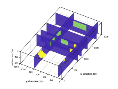
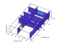
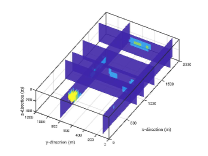
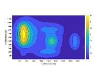
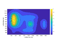
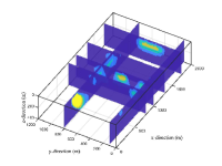
For the validation of the algorithms, we pick a volume structure with a number of boxes of different dimensions, and a six-layer dipping dike. The same structure is used for generation of the gravity and magnetic potential field data. For gravity data the densities of all aspects of the structure are set to $1$, with the homogeneous background set to $0$. For the magnetic data, the dipping dike, one extended well and one very small well have susceptibilities $.06$. The three other structures have susceptibilities set to $.04$. The distinction between these structures with different susceptibilities is illustrated in the illustration of the iso-structure in Figure 2(a) and the cross-section in Figure 2(b).

(a) Iso-surface of the volume structure.

(b) Cross-section of the volume structure.

Figure 2. The basic volume structure within the domain of size $2000\times 1200\times 400$. The extent of each structure is shown by the shadow on the base of the volume. The same structure is used for the results using the padded domain.

The domain volume is discretized in $x$, $y$ and $z$ into the number of blocks as indicated by triples $(s_{x},s_{y},n_{z})$ with increasing resolution for increasing values of these triples. They are generated by taking $(s_{x},s_{y},n_{z})=(25,15,2)$, and then scaling each dimension by scaling factor $\ell\geq 4$ for the test cases, correspondingly, $s_{x}s_{y}=375$ is scaled by $\ell^{2}$ with increasing $\ell$, yielding a minimum problem size with $m=6000$ and $n=48000$. The grid sizes are thus given by the triples $(\Delta_{x},\Delta_{y},\Delta_{z})=(2000/s_{x},1200/s_{y},400/n_{z})$. The problem sizes considered for each simulation are detailed in Table 2. For padding we compare the case with $\mathrm{pad}=0\%$ and $\mathrm{pad}=5\%$ padding across $x$ and $y$ dimensions. These are rounded to the nearest integer yielding $p_{x_{\texttt{L}}}=p_{x_{\texttt{R}}}=\texttt{round}(\mathrm{pad}\,s_{x})$, and $n_{x}=s_{x}+2\,\texttt{round}(\mathrm{pad}\,s_{x})$. $n_{y}$ is calculated in the same way, yielding $n=(s_{x}+2\,\texttt{round}(\mathrm{pad}\,s_{x}))(s_{y}+2\,\texttt{round}(\mathrm{pad}\,s_{y}))n_{z}$. Certainly, the choice to use $\mathrm{pad}=5\%$ is quite large, but is chosen to demonstrate that the solutions obtained using the 2DFFT are robust to boundary conditions, and thus not impacted by the restriction due to lack of padding or very small padding.

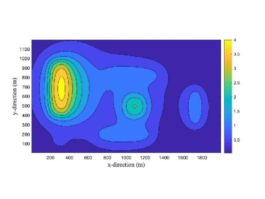
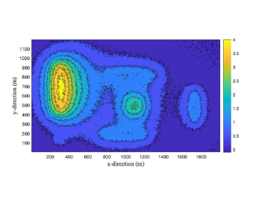
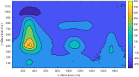
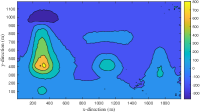
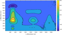
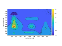
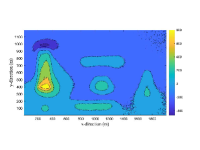
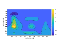
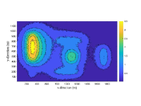
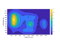
For these structures and resolutions, noisy data are generated as given in (18) to yield an SNR of approximately $24$ across all scales as calculated using (19). This results in different choices of $\tau_{1}$ and $\tau_{2}$ for each problem size and dependent on the gravity or magnetic data case, denoted by $(\tau_{1}^{\mathrm{g}},\tau_{2}^{\mathrm{g}})$ and $(\tau_{1}^{\mathrm{m}},\tau_{2}^{\mathrm{m}})$, respectively. In all cases we use $\tau_{1}^{\mathrm{g}}=\tau_{1}^{\mathrm{m}}=.02$ and adjust $\tau_{2}$. The simulations for the choices of $\tau_{2}^{\mathrm{g}}$ and $\tau_{2}^{\mathrm{m}}$ for increasing problem sizes are detailed in Table 1. As an example we illustrate the true and noisy data for gravity and magnetic data, when $\ell=12$, in Figure 3.

$\ell$	$(s_{x},s_{y},n_{z})$	$m$	$n$	$n_{\mathrm{pad}}$	$\tau_{2}^{\mathrm{g}}$	$\tau_{2}^{\mathrm{m}}$	SNRg	SNRm
$4$	$(100,60,8)$	$6000$	$48000$	$58080$	$.0138$	$.0081$	$24.0$	$24.0$
$5$	$(125,75,10)$	$9375$	$93750$	$113710$	$.0147$	$.0083$	$24.0$	$24.0$
$6$	$(150,90,12)$	$13500$	$162000$	$199200$	$.0133$	$.0074$	$24.0$	$24.0$
$7$	$(175,105,14)$	$18375$	$257250$	$310730$	$.0133$	$.0070$	$24.0$	$24.0$
$8$	$(200,120,16)$	$24000$	$384000$	$464640$	$.0133$	$.0071$	$24.0$	$24.1$
$9$	$(225,135,18)$	$30375$	$546750$	$662450$	$.0133$	$.0069$	$24.0$	$24.0$
$10$	$(250,150,20)$	$37500$	$750000$	$916320$	$.0132$	$.0070$	$24.0$	$24.0$
$11$	$(275,165,22)$	$45375$	$998250$	$1206500$	$.0135$	$.0075$	$24.0$	$24.0$
$12$	$(300,180,24)$	$54000$	$1296000$	$1568160$	$.0135$	$.0075$	$24.0$	$24.0$

Table 2. Dimensions of the volume used in the experiments with scaling of the small problem size $(25,15,2)$ by scale factor $\ell$ in each dimension. $m$ and $n$ are the dimensions of the measurement vector and the volume domain, respectively, $G\in\mathcal{R}^{m\times n}$. Here $m=s_{x}s_{y}=375\ell^{2}$ and $n=mn_{z}$ where $n_{x}=s_{x}$ and $n_{y}=s_{y}$ without padding. Here, we use $n_{\mathrm{pad}}=n_{x}n_{y}n_{z}$ to denote the volume dimension $n$ with $5\%$ padding, using $n_{x}=s_{x}+2\,\texttt{round}(\mathrm{pad}\,s_{x})$ and $n_{y}=s_{y}+2\,\texttt{round}(\mathrm{pad}\,s_{y})$ for padding obtained using a percentage, $\mathrm{pad}$, on each side of the domain so that $p_{x_{\texttt{L}}}=p_{x_{\texttt{R}}}=\texttt{round}(\mathrm{pad}\,s_{x})$, and similarly for $s_{y}$. .

(a) True gravity anomaly

(b) Noisy gravity anomaly

(c) True magnetic anomaly

(d) Noisy magnetic anomaly

Figure 3. The calculated true and noisy anomalies for the volume structure given in Figure 2(a), where the units are mGal and nT for gravity and magnetic data, respectively. The anomalies used for the inversion using the padded domain are exactly the same as given here.

3.3. Numerical Results

The validation and analysis of the algorithms for the inversion of the potential field data is presented in terms of (i) the cost per iteration of the algorithm (Section 3.3.1), (ii) the total cost to convergence of the algorithm (Section 3.3.2), and (iii) the quality of the obtained solutions, (Section 3.3.3). Supporting quantitative data that summarize the illustrated results are presented as Tables in B.

3.3.1. Comparative cost of RSVD and GKB algorithms per IRLS iteration

We investigate the computational cost, as measured in seconds, for one iteration of the inversion algorithm using both the direct multiplications using matrix $G$, respectively, $G^{T}$, and the circulant embedding, for the resolutions up to $\ell=6$ that are indicated in Table 2, using both the RSVD and GKB algorithms, and for both gravity and magnetic data. For fair comparison, all the timing results that are reported use Matlab release 2019b implemented on the same iMac $4.2$GHz Quad-Core Intel Core i7 with $32$GB RAM. In this environment, the size of the matrix $G$ is too large for effective memory usage when $\ell>6$. The details of the timing results for one step of the IRLS algorithm are illustrated in Figures 4-7, with the specific values for the magnetic data case, given in Table 4.

(a) Running time magnetic: GKB.

(b) Running time magnetic: RSVD.

(c) Running time gravity: GKB.

(d) Running time gravity: RSVD.

Figure 4. Running time in seconds for one iteration of the inversion algorithm for the inversion of magnetic and gravity data, without padding the volume domain. Problems are of increasing size, as indicated by the $x-$axis for triples $[n_{x},n_{y},n_{z}]$ and increasing projection size $t$ ($y-$axis using $\log$ scale) determined by fractions of $m=s_{x}s_{y}$. In Figures 4(a) and 4(c) the running time for the GKB algorithm using $t_{p}=\texttt{floor}(1.05t)$ (an oversampling percentage $5\%$), for the magnetic and gravity problems respectively. In Figures 4(b) and 4(d) the equivalent running times using the RSVD algorithm with one power iteration. In these plots the solid symbols represent the timing for one iteration of the algorithm using the 2DFFT and the open symbols represent the timing for the same simulation using $G$ directly. Matrix $G$ for problem size $\ell=7$, which corresponds to triple $[175,105,14]$, requires too much memory for implementation in the specific computing environment.

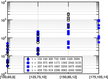
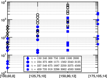
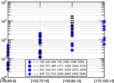
Figure 4 provides an overview of the computational cost with increasing projection size $t$, for a given $m$, when the algorithm is implemented using $G$ directly, or using the 2DFFT. These costs exclude the cost of generating $G$. In these plots, we use the open symbols for calculations using $G$ and solid symbols when using the 2DFFT. The same symbols are used for each choice of $t$ and $\ell$. An initial observation, confirming expectation, is that the timings for equivalent problems and methods, are almost independent of whether the potential field data are gravity or magnetic, comparing Figures 4(a)-4(b) with Figures 4(c) and 4(d). The lack of entries for triple $[175,105,14]$ indicates that the matrix $G$ is too large for the operations, $\ell=7$. With increasing $\ell$, (increasing values of the triples along the $x-$axis), it can also be observed that the open symbols are more spread out vertically, confirming that the algorithms using $G$ directly are more expensive for problems at these resolutions.

(a) magnetic data: $\texttt{Cost}_{\texttt{G}}/\texttt{Cost}_{\texttt{2DFFT}}$.

(b) gravity data: $\texttt{Cost}_{\texttt{G}}/\texttt{Cost}_{\texttt{2DFFT}}$.

Figure 5. Relative computational cost for one iteration of the IRLS algorithm using $G$ directly as compared to the 2DFFT, as indicated by $\texttt{Cost}_{\texttt{G}}/\texttt{Cost}_{\texttt{2DFFT}}$, for the data presented in Figure 4, for the magnetic and gravity problems, Figures 5(a)-5(b). Here, the values for the relative cost that are less than $1$, below the horizontal line at $y=1$, indicate that it is more efficient to use $G$ directly. Values that are greater than $1$ indicate that it is more efficient to use the 2DFFT. Open symbols indicate the GKB algorithm and solid symbols the RSVD algorithm. In each case the given plots for a fixed $\ell$ are for increasing projection size $t$ as given by $m/s$ for the selections of $t$ as used in Figure 4.

In Figure 5 we plot the relative computational costs for one iteration of the IRLS algorithm using the matrix $G$ as compared to the algorithm using the 2DFFT, as indicated by $\texttt{Cost}_{\texttt{G}}/\texttt{Cost}_{\texttt{2DFFT}}$, for the data presented in Figure 4. Along the $x-$axis we give the size $t$ used for the projected problem in terms of the ratio $m/s$. The lines with solid blue symbols are for results using the RSVD algorithm, and the open black symbols are for the GKB algorithm. Here, the values for the relative cost that are less than $1$, below the horizontal green line at $y=1$, indicate that for the specific algorithm it is more efficient to use $G$ directly. Values that are greater than $1$ indicate that it is more efficient to use the 2DFFT for the given algorithm and problem size. It is apparent that it is not beneficial to use the 2DFFT for the smaller scale implementation of the RSVD algorithm, when $\ell=4$ or $5$. But the situation is completely reversed using the GKB algorithm for all choices of $\ell$ and the RSVD algorithm for $\ell\geq 6$. Thus, the relative gain in reduced computational cost, by using the 2DFFT depends on the algorithm used within the IRLS inversion algorithm. The decrease in efficiency for a given size problem, fixed $\ell$ but increasing size $t$ (in the $x-$axis), is explained by the theoretical discussion relating to equations (13)-(14). As $t$ increases the impact of the efficient matrix multiplication using the 2DFFT is reduced. Again the gravity and magnetic data results are comparable.

(a) magnetic data: $\texttt{Cost}_{\texttt{GKB}}/\texttt{Cost}_{\texttt{RSVD}}$.

(b) gravity data: $\texttt{Cost}_{\texttt{GKB}}/\texttt{Cost}_{\texttt{RSVD}}.$

Figure 6. The relative computational cost for one iteration of the IRLS algorithm for inversion using the GKB as compared to the RSVD algorithm ($\texttt{Cost}_{\texttt{GKB}}/\texttt{Cost}_{\texttt{RSVD}}$), for given $\ell$ and projected size $t$. In each case the given plots for a fixed $\ell$ are for increasing projection size $t$ as given by $m/s$ as in Figure 5. The horizontal line at $y=1$ represents the data for which the costs are the same, independent of whether using the RSVD or GKB algorithms. The GKB is more efficient when $t$ is maintained small, $s=40$, $25$ and $20$. The gain in using the GKB decreases, however, as $\ell$ increases. For small $\ell$ and $t$, the estimates confirm the computational cost estimates in (13)-(14), but for larger projection sizes $t$, the RSVD is more efficient. In Figure 6(a) the relative costs are also included for $\ell=8$ and $\ell=9$, where $t\leq 5000$.

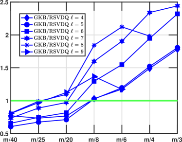
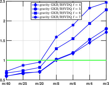
Figure 4 provides no information on the relative costs of the GKB and RSVD algorithms with increasing $\ell$, independent of the use of the 2DFFT. Figure 6 shows the relative computational costs, $\texttt{Cost}_{\texttt{GKB}}/\texttt{Cost}_{\texttt{RSVD}}$. Note that Figure 6(a) also includes results for larger problems. These plots demonstrate that the relative costs for a single iteration are not constant across all $t$ with the GKB generally cheaper for smaller $t$, and the RSVD cheaper for larger $t$. These results confirm the analysis of the computational cost in terms of flops provided in (13)-(14) for small $t$. The relative computational costs increase from roughly $0.6$ to $2.5$, increasing with both $\ell$ and $t$. Still, this improved relative performance of RSVD with increasing $\ell$ and $t$ appears to violate the flop count analysis in (13)-(14). As discussed in Section 2.5, this is a feature of the implementation. While RSVD is implemented using the Matlab builtin function qr which uses compiled code for faster implementation, GKB only uses builtin operations for performing the MGS reorthogonalization of the basis matrices $A_{t_{p}}$ and $H_{t_{p}}$. Once again results are comparable for inversion of both gravity and magnetic data sets.

(a) Running time (padded): GKB.

(b) Running time (padded): RSVD.

(c) $\texttt{Cost}_{\texttt{G}}/\texttt{Cost}_{\texttt{2DFFT}}$ (Padded).

(d) $\texttt{Cost}_{\texttt{GKB}}/\texttt{Cost}_{\texttt{RSVD}}$ (Padded).

Figure 7. In Figures 7(a)-7(b) the running time in seconds for one iteration of the inversion algorithm for the inversion of magnetic data, for the same problems as in Figure 4(a) and 4(b) but with padding, $\mathrm{pad}=5\%$, added to the volume domain. Problems are of increasing size, as indicated by the $x-$axis for triples $[n_{x},n_{y},n_{z}]$ and increasing projection size $t$ ($y-$axis using $\log$ scale) determined by fractions of $m=s_{x}s_{y}$. In these plots the solid symbols represent the timing for one iteration of the algorithm using the 2DFFT and the open symbols represent the timing for the same simulation without using the 2DFFT for the kernel operations. In Figure 7(c) the relative costs for these results, as also provided in Figure 5(a) for the case without padding, and in Figure 7(d) the relative costs of the two algorithms with the 2DFFT, as in Figure 6(a) without padding.

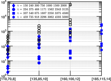
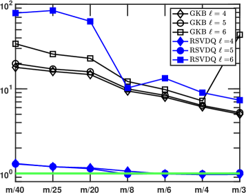
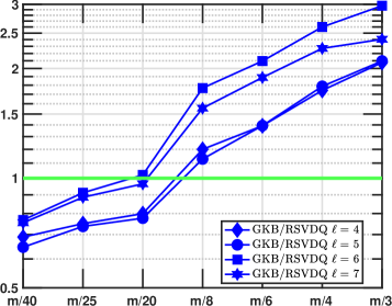
Figure 7 summarizes magnetic data timing results from Table 4 for domains which are padded with $5\%$ padding in $x$ and $y$ directions. Data illustrated in Figures 7(a)-7(b) are equivalent to the results presented in Figures 4(a)-4(b), but with padded volume domains. Again these results show the open symbols are more spread out vertically, for increasing $\ell$, confirming that the algorithms using $G$ directly are more expensive for problems at these resolutions, with greater impact when using the GKB algorithm for small $\ell$. This is further confirmed in Figure 7(c), equivalent to Figure 5(a), showing that the computational cost of performing one step of the IRLS algorithm using matrix $G$ directly, is always greater than that using the 2DFFT. This is more emphasized for the GKB algorithm. The relative costs shown in Figure 7(d), equivalent to Figure 6(a), again shows that the GKB algorithm is cheaper for small $t$ when $\ell$ is small. But as the problem size increases and the projected problem size also increases, it is more efficient to use the RSVD algorithm, consistent with the observations for the unpadded domains.

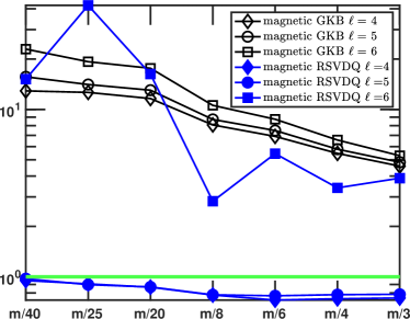
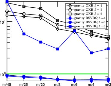
3.3.2. Comparative cost of RSVD and GKB algorithms to convergence

(a) magnetic $\texttt{Cost}_{\texttt{GKB}}/\texttt{Cost}_{\texttt{RSVD}}.$

(b) gravity $\texttt{Cost}_{\texttt{GKB}}/\texttt{Cost}_{\texttt{RSVD}}.$

Figure 8. Computational cost to convergence of the IRLS  algorithm for inversion using the GKB as compared to the RSVD algorithm, $\texttt{Cost}_{\texttt{GKB}}/\texttt{Cost}_{\texttt{RSVD}}$, for the magnetic and gravity problems respectively, in Figures 8(a)-8(b).

The computational cost of the IRLS algorithm for solving the inversion problem to convergence depends on the choice of $t$, the choice of GKB or RSVD algorithms, and whether solving the magnetic or the gravity problem. In Table 5 we report the timing results for the inversion of gravity and magnetic data for problems of increasing size $\ell$ and projected spaces of sizes $t_{p}$. The relative total computational costs to convergence, $\texttt{Cost}_{\texttt{GKB}}/\texttt{Cost}_{\texttt{RSVD}}$, (the last two columns in Table 5) are illustrated via Figures 8(a)-8(b), for the magnetic and gravity results, respectively. There is a distinct difference between the two problems. The results in Figure 8(a) for the magnetic problem demonstrate a strong preference for the use of the GKB algorithm, except for large $t$, $t=\texttt{floor}(m/3)$. In contrast, the RSVD algorithm is always most efficient for the solution of the gravity problem, which is consistent with the conclusion presented in Vatankhah et al. [2018] for RSVD without power iteration. Moreover, the data presented in Table 7 for the gravity problem, indicate that the RSVD algorithm generally converges more quickly and yields a smaller relative error. Furthermore, if based entirely on the calculated RE, the results suggest that good results can be achieved for relatively small $t$ as compared to $m$, certainly $s\gtrsim 8$ leads to generally acceptable error estimates, and in contrast to the case without the power iteration, here with power iteration, the errors using the GKB are generally larger for comparable choices of $t$.

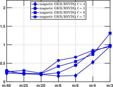
For the magnetic data, the results in Table 6 demonstrate that the RSVD algorithm generally requires more iterations than the GKB algorithm, and that the obtained relative errors are then comparable, or slightly larger. This is then reflected in Figure 8(a) that the GKB algorithm is most efficient. Referring back to Table 6, it is the case that the RSVD algorithm often reaches the maximum number of iterations, $K=25$, without convergence, when GKB has converged in less than half the number of iterations, when $t$ is small relative to $m$, $t=\texttt{floor}(m/s)$ with $s=40$, $25$ and $20$. This verifies that the RSVD needs to take a larger projected subspace $t$ in order to capture the required dominant spectral space when solving the magnetic problem, as compared to the gravity problem, and confirms the conclusions presented in Vatankhah et al. [2020a]. On the other hand, the use of the GKB as compared to the RSVD was not discussed in Vatankhah et al. [2020a]. Our results now lead to a new conclusion concerning these two algorithms for solving the magnetic data inversion problem. In particular, the results suggest that the GKB algorithm be adopted for inversion of magnetic data. Further, the results suggest that the relative error obtained using the GKB generally decreases with increasing $t$, and that it is necessary to use subspaces with $t$ at least as large as $\texttt{floor}(m/8)$. It remains to verify these assertions by illustrating the results of the inversions and the predicted anomalies for a selection of cases.

3.3.3. Illustrating Solutions with Increasing $\ell$ and $t$

We first compare a set of solutions for which the timing results were compared in Section 3.3.2. Figure 9 illustrates the predicted anomalies and reconstructed volumes for gravity data inverted by both algorithms, with resolutions given by $\ell=4$ and $\ell=7$ with $t=\texttt{floor}(m/8)$ and $t=\texttt{floor}(m/4)$. For the cases using $\ell=4$ it can be seen that the predicted anomalies are generally less accurate than with $\ell=7$. Moreover, there is little deterioration in the anomaly predictions when using $t=\texttt{floor}(m/8)$ instead of $t=\texttt{floor}(m/4)$, except that the results with the GKB show more residual noise. On the other hand, it is more apparent from consideration of the reconstructed volumes shown in Figures 9(i)-9(p) that the RSVD algorithm does yield better results in all cases, and specifically the high resolution $\ell=7$ results are very good, even using $t=\texttt{floor}(m/8)$. When including the consideration of the computational cost, it is clear that if using $\ell=7$ it is sufficient to use $t=\texttt{floor}(m/8)$ and the RSVD algorithm, but that a reasonable result may even be obtained using the same algorithm but with $\ell=4$ and requiring less than $5$ minutes of compute time.

(a) GKB: $\ell=4$,        $\quad t=750$, $(9,248\textrm{s})$.

(b) $\ell=4$, $t=1500$, $(7,494\textrm{s})$.

(c) $\ell=7$, $t=2296$, $(11,5732\textrm{s})$.

(d) $\ell=7$, $t=4593$, $(8,12347\textrm{s})$.

(e) RSVD: $(6,216\textrm{s})$.

(f) $(6,436\textrm{s})$.

(g) $(7,3311\textrm{s})$.

(h) $(7,6979\textrm{s})$.

(i) GKB: $(.76,.90)$.

(j) $(.64,.96)$.

(k) $(.75,.81)$.

(l) $(.70,1.00)$.

(m) RSVD: $(.57,.96)$.

(n) $(.57,.93)$.

(o) $(.60,.95)$.

(p) $(.61,.91)$.

Figure 9. For gravity data the predicted anomalies obtained using GKB in Figures 9(a)-9(d) and RSVD in Figures 9(e)-9(h), with the corresponding reconstructed volumes in Figures 9(i)-9(l) and Figures 9(m)-9(p), respectively. In each case the first row for GKB indicates the choices of $\ell$ and $t$ in each column. The choices $t=750$ and $t=1500$ for $\ell=4$, and with $t=2296$ and $t=4593$ for $\ell=7$, correspond to $t=\texttt{floor}(m/8)$ and $t=\texttt{floor}(m/4)$ for $(m,n)=(6000,48000)$ and $(18375,257250)$, respectively. Given are the pairs $(K,\texttt{Cost}\textrm{s})$, (number of iterations to convergence and computational cost in seconds) in the captions of the anomalies, and $(\texttt{RE},\chi^{2}/(m+\sqrt{2m}))$ in the captions of the reconstructions. Results for all cases are summarized in Table 7 with timings in Table 5. The units for the anomalies are mGal.

The results for the inversion of the magnetic data are illustrated in Figure 10 for the same cases as for the inversion of gravity data in illustrated in Figure 9. Now, in contrast to the gravity results, the predicted anomalies are in good agreement with the true data for the results obtained using the GKB algorithm, with apparently greater accuracy for the lower resolution solutions, $\ell=4$ for both choices of $t$. On the other hand, the predicted magnetic anomalies are less satisfactory for small $\ell$ and $t$ but acceptable for large $\ell$. Then, considering the reconstructed volumes, there is a lack of resolution for $\ell=4$ which is evidenced by the loss of the small well near the surface, which is seen when $\ell=7$ for both cases of $t$, when using the GKB. The other structures in the domain are also resolved better with $\ell=7$, but there is little gain from using $t=\texttt{floor}(m/4)$ over $t=\texttt{floor}(m/8)$. Then, considering the reconstructions obtained using the RSVD algorithm, while it is clear that the result with $\ell=4$ and small $t$ is unacceptable, the anomaly and reconstructed volume with $\ell=4$ and $t=\texttt{floor}(m/4)$ is acceptable and achieved in reasonable time, approximately $11$ minutes, far faster than using $\ell=7$ with GKB. Thus, this may contradict the conclusion that one should use the GKB algorithm within the magnetic data inversion algorithm. If there is a large amount of data and a high resolution volume is required, then it is important to use GKB in order to limit computational cost. Otherwise, it can be sufficient to use the RSVD provided $t\geq\texttt{floor}(m/8)$ for a coarser resolution solution obtained at reasonable computational cost.

(a) GKB: $\ell=4,t=750$, $(5,136\textrm{s})$.

(b) $\ell=4,t=1500$, $(5,343\textrm{s})$.

(c) $\ell=7,t=2296$, $(7,3809\textrm{s})$.

(d) $\ell=7,t=4593$, $(7,10979\textrm{s})$.

(e) RSVD: $(25,883\textrm{s})$.

(f) $(9,650\textrm{s})$.

(g) $(14,6618\textrm{s})$.

(h) $(13,12949\textrm{s})$.

(i) GKB: $(.63,.90)$.

(j) $(.63,.91)$.

(k) $(.67,.90)$.

(l) $(.68,.92)$.

(m) RSVD: $(.64,1.11)$.

(n) $(.63,.93)$.

(o) $(.70,.99)$.

(p) $(.69,.90)$.

Figure 10. For magnetic data the predicted anomalies obtained using GKB in Figures 10(a)-10(d) and RSVD in Figures 10(e)-10(h), with the corresponding reconstructed volumes in Figures 10(i)-10(l) and Figures 10(m)-10(p), respectively. In each case the first row for GKB indicates the choices of $\ell$ and $t$ in each column. The choices $t=750$ and $t=1500$ for $\ell=4$, and with $t=2296$ and $t=4593$ for $\ell=7$, correspond to $t=\texttt{floor}(m/8)$ and $t=\texttt{floor}(m/4)$ for $(m,n)=(6000,48000)$ and $(18375,257250)$, respectively. Given are the pairs $(K,\texttt{Cost}\textrm{s})$, (number of iterations to convergence and computational cost in seconds) in the captions of the anomalies, and $(\texttt{RE},\chi^{2}/(m+\sqrt{2m}))$ in the captions of the reconstructions. Results for all cases are summarized in Table 6 with timings in Table 5. The units for the anomalies are nT.

We now investigate the quality of solutions obtained for magnetic data using higher resolution data sets, and both GKB and RSVD algorithms to assess which algorithm is best suited for such larger problems. In these cases we pick $t=\texttt{floor}(m/20)$, to assess quality with a necessarily restricted subspace size as compared to the size of the given data set. Results using $\ell=11$ with $t=2268$ and $\ell=12$ with $t=2700$, corresponding to $m=45375$ and $n=998250$, and $m=54000$ and $n=1296000$, respectively, are illustrated in Figure 11. For these large scale problems, the memory becomes too large for implementation on the environment with just $32$GB RAM. Thus, these timings are for an implementation using a desktop computer with the Intel(R) Xeon (R) Gold 6138 CPU 2.00GHz chip and with Matlab release 2019b. Comparing the results between $m=45375$ and $m=54000$ ($\ell=11$ and $\ell=12$) it can be seen that the predicted anomalies are always better for the larger problem, and in particular the result shown in Figure 11(e) shows greater artifacts when using RSVD. The obtained reconstruction for this case, shown in Figure 11(g) is, however, acceptable. Overall, trading off between computational cost and solution quality, there seems little gain in using $\ell=12$ and the results with $\ell=11$ obtained with the GKB algorithm in $227$ minutes (nearly $4$ hours) are suitable. These results also show that it is sufficient to use a relatively smaller projected space, $t=\texttt{floor}(m/20)$ when $m$ is larger. Indeed, notice that even in these cases the largest matrix required by both algorithms is of size $n\times t_{p}$ and requires $17.7$GB and $27.4$GB, for $\ell=11$ and $\ell=12$, respectively. Effectively, it is this large memory requirement that limits the given implementation using either GKB or RSVD for larger size problems.

(a) $11:(9,13595\textrm{s})$.

(b) $12:(8,21649\textrm{s})$.

(c) $11:(.74,.98)$.

(d) $12:(.74,.92)$.

(e) $(15,21266\textrm{s})$.

(f) $(16,41981\textrm{s})$.

(g) $(.74,.99)$.

(h) $(.73,.98)$.

Figure 11. The magnetic anomalies and reconstructed volumes using the GKB and RSVD algorithms in Figures 11(a)-11(d) and 11(e)-11(h), respectively. The first row indicates the choice of $\ell=11$, for which $t=2268=\texttt{floor}(m/20)$, $m=45375$ and $n=998250$ and oversampled projected problem of size $2381$, or $\ell=12$, with $t=2700=\texttt{floor}(m/20)$, $m=54000$ and $n=1296000$, and oversampled projected problem of size $2835$. Given are the pairs $(K,\texttt{Cost}\textrm{s})$, (number of iterations to convergence and computational cost in seconds) in the captions of the anomalies, and $(\texttt{RE},\chi^{2}/(m+\sqrt{2m}))$ in the captions of the reconstructions. The units for the anomalies are nT.

Numerical experiments for the inversion of gravity data, similar to the testing for the magnetic data, demonstrates that indeed the RSVD algorithm with power iteration is to be preferred for the inversion of gravity data, yielding acceptable solutions at lower cost than when using the GKB algorithm. Representative results are detailed in Figure 12 for the same parameter settings as given in Figure 11 for the magnetic problem.

(a) $11:(21,30833\textrm{s})$.

(b) $12:(21,59837\textrm{s})$.

(c) $11:(1.02,.76)$.

(d) $12:(1.00,.78)$.

(e) $(8,11779\textrm{s})$.

(f) $(8,30212\textrm{s})$.

(g) $(.61,1.00)$.

(h) $(.59,.99)$.

Figure 12. The gravity anomalies and reconstructed volumes using the GKB and RSVD algorithms in Figures 12(a)-12(d) and 12(e)-12(h), respectively. The first row indicates the choice of $\ell=11$, for which $t=2268=\texttt{floor}(m/20)$, $m=45375$ and $n=998250$ and oversampled projected problem of size $2381$, or $\ell=12$, with $t=2700=\texttt{floor}(m/20)$, $m=54000$ and $n=1296000$, and oversampled projected problem of size $2835$. Given are the pairs $(K,\texttt{Cost}\textrm{s})$, (number of iterations to convergence and computational cost in seconds) in the captions of the anomalies, and $(\texttt{RE},\chi^{2}/(m+\sqrt{2m}))$ in the captions of the reconstructions. The units for the anomalies are mGal.

3.4. Real Data

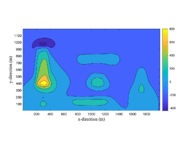
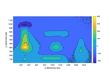
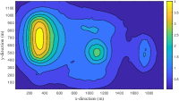
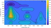
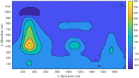
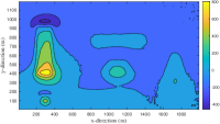
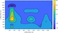
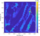
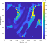
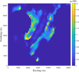
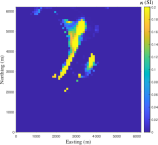
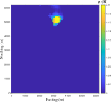
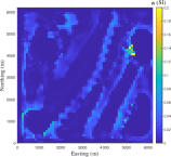
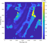
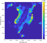
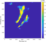
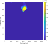
For validation of the simulated results on a practical data set we apply the GKB algorithm for the inversion of a magnetic field anomaly that was collected over a portion of the Wuskwatim Lake region in Manitoba, Canada. This data set was discussed in Pilkington [2009] and also used in Vatankhah et al. [2020a] for inversion using the RSVD algorithm with a single power iteration. Further details of the geological relevance of this data set is given in these references. Moreover, its use makes for direct comparison with these existing results. Here we use a grid of $62\times 62=3184$ measurements at $100$m intervals in the East-North direction with padding of $5$ cells yielding a horizontal cross section of size $72\times 72$ in the East-North directions. The depth dimension is discretized with $\Delta z=100$m, yielding a regular cube, to $\Delta z=8$m for rectangular prisms with a smaller edge length in the depth dimension for a total depth of $2000$m, and providing increasing values of $n$ from $103680$ to $1238976$ as detailed in Table 3. The given magnetic anomaly is illustrated in Figure 13(a).

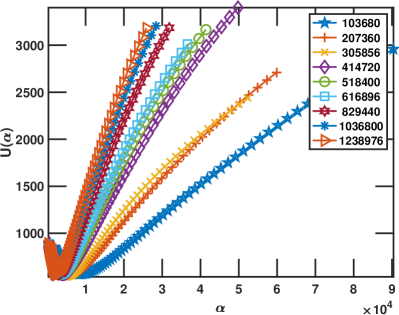
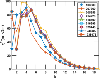
In each inversion the GKB algorithm is run with $t=480$, corresponding to $t=\texttt{floor}(m/8)$, where $m=3184$ and oversampled projected space of size $504$, and a noise distribution based on (18) is employed using $\tau_{1}=.02$ and $\tau_{2}=.018$. All inversions converge to the tolerance $\chi^{2}/(m+\sqrt{2m}))<1$ in no more than $19$ iterations for all problem sizes, as given in Table 3. The computational cost measured in seconds is also given in Table 3 and demonstrates that it is feasible to invert for large parameter volumes, in times ranging from just under $5$ minutes for the coarsest resolution, to just over $73$ minutes for the volume with the highest resolution. Here the computations are performed on a MacBook Pro laptop with 2.5 GHz Dual-Core Intel Core i7 chip and $16$GB memory. In Figure 14(a) we show that the UPRE function has a well-defined minimum at the final iteration for all resolutions, and in Figure 14(b) that the convergence of the scaled $\chi^{2}$ value is largely independent of $n$. The final regularization parameter $\alpha^{(K)}$ decreases with increasing $n$, while the initial $\alpha$ found using (15) increases with $n$, as reported in Table 3.

(a) Given anomaly.

(b) Predicted: $n=103680$.

(c) Predicted: $n=1238976$.

Figure 13. The given magnetic anomaly in Figure 13(a) and the obtained predicted anomalies for the inversion using the parameters for the first and last lines of data in Table 3 in Figures 13(b)-13(c), respectively.

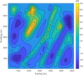
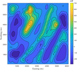
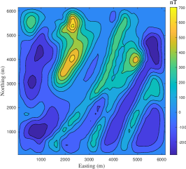
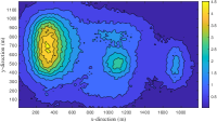
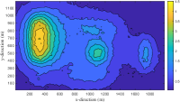
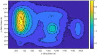
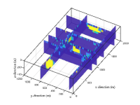
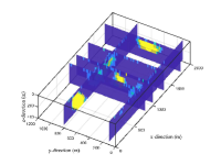
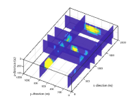
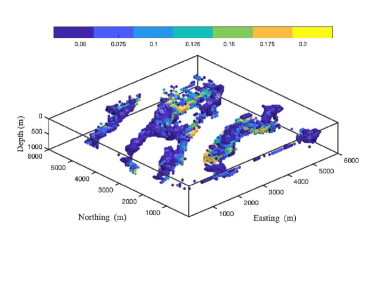
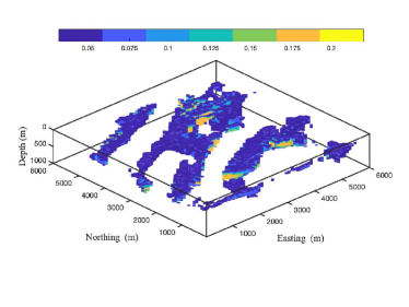
Results of the inversion, for the coarsest and finest resolutions are presented in Figures 13, 15 and 16, for anomalies, reconstructed volumes, and depth slices through the volume domain, respectively. First, from Figures 13(b)-13(c), as compared to Figure 16b in Vatankhah et al. [2020a], we see that the predicted anomalies provide better agreement to the measured anomaly, with respect to structure and the given values. Moreover, more structure is seen in the volumes presented in Figures 15(a)-15(b) as compared to Figure19 Vatankhah et al. [2020a], and the increased resolution provides greater detail in Figure 15(b)as compared to Figure 15(a). Here the volumes are presented for the depth from $0$ to $1000$m only, but it is seen in Figures 16(e) and 16(j), which are the slices at depth $1100$m, that there is little structure evident at greater depth. Comparing the depth slices for increasing depth, we see that the use of the higher resolution leads to more structure at increased depth. Moreover, the results are consistent with those presented in Vatankhah et al. [2020a] for the use of the RSVD for a projected size $t=1100$ as compared to $t=480$ used here. It should also be noted that the RSVD algorithm with one power iteration does not converge within $50$ steps, under the same configurations for $m$, $n$ and $t$.

$n$	$n_{z}$	$\Delta z$	$K$	$\alpha^{(1)}$	$\alpha^{(K)}$	${\chi^{2}}/{(m+\sqrt{2m})}$	$\textrm{Cost}(s)$
$103680$	$20$	$100$	$17$	$4.60e+05$	$8558$	$0.87$	$334$
$207360$	$40$	$50$	$18$	$5.36e+06$	$5887$	$0.90$	$754$
$305856$	$59$	$33$	$19$	$2.07e+07$	$4930$	$0.70$	$1126$
$414720$	$80$	$25$	$18$	$6.09e+07$	$4116$	$0.95$	$1513$
$518400$	$100$	$20$	$18$	$1.33e+08$	$3701$	$0.94$	$2018$
$616896$	$119$	$16$	$18$	$2.43e+08$	$3386$	$0.90$	$2095$
$829440$	$160$	$12$	$18$	$6.90e+08$	$2933$	$0.95$	$3091$
$1036800$	$200$	$10$	$18$	$1.51e+09$	$2627$	$0.95$	$3690$
$1238976$	$239$	$8$	$18$	$2.80e+09$	$2396$	$0.96$	$4389$

Table 3. Inversion of magnetic data as illustrated in Figure 13 for $m=3844$ on a grid of $62\times 62$ stations, with $\Delta x=\Delta y=100$m and padding of $5$ cells in both $x$ and $y$-directions, yielding blocks of size $n_{r}=5184$. The inversion uses the GKB algorithm with $t=480$ ($\texttt{floor}(m/8)$) and $t_{p}=504$. The noise in the algorithm uses (18) as given for the simulations with $\tau_{1}=.02$ and $\tau_{2}=.018$. These results are obtained using a MacBook Pro laptop with 2.5 GHz Dual-Core Intel Core i7 chip and $16$GB memory.

(a) Regularization function for $K$.

(b) $\chi^{2}$ with $k$.

Figure 14. The plot of the regularization function $U(\alpha)$ for the UPRE algorithm, at the final iteration $K$ for increasing values of $n$ as indicated in Table 3 in Figure 14(a) and the progression of the scaled $\chi^{2}$ estimate as a function of iteration $k$ and for increasing $n$ in Figure 14(b).

(a) Iso-surface using $n=103680$.

(b) Iso-surface using $n=1238976$.

Figure 15. The reconstructed volumes showing parameters $\kappa>0.05$ and depth from $0$ to $1000$, corresponding to the predicted anomalies in Figure 13.

(a) $300$m

(b) $500$m

(c) $700$m

(d) $900$m

(e) $1100$m

(f) $300$m

(g) $500$m

(h) $700$m

(i) $900$m

(j) $1100$m

Figure 16. Slices through the volumes illustrated in Figure 15 for depths $300$, $500$, $700$, $900$ and $1100$, for $n=103680$ in Figures 16(a)-16(e) and for $n=1238976$ in Figures 16(f)-16(j).

4. Conclusions and Future Work

Two algorithms, GKB and RSVD, for the focused inversion of potential field data with all operations for the sensitivity matrix $G$ implemented using a fast 2DFFT algorithm have been developed and validated for the inversion of both gravity and magnetic data sets. The results show first that it is distinctly more efficient to use the 2DFFT for operations with matrix $G$ rather than direct multiplication. This is independent of algorithm and data set, for all large scale implementations considered. Moreover, the implementation using the 2DFFT makes it feasible to solve these large scale problems on a standard desktop computer without any code modifications to handle multiple cores or GPUs, which is not possible due to memory constraints when $m$ and $n$ increase. While both algorithms are improved with this implementation, the results show that the impact on the GKB efficiency is greater than that on the RSVD efficiency. A theoretical analysis of the computational cost of each algorithm for a single iterative step demonstrates that the GKB should be faster, but this is not always realized in practice as the problem size increases, with commensurate increase in the size of the projected space. Then, the efficiency of GKB deteriorates, and the advantage of using builtin routines from Matlab for the RSVD algorithm is crucial.

When considering the computational cost to convergence for both algorithms, which also then includes the cost due to the requiring projected spaces that are of reasonable size relative to $m$, the results confirm earlier published results that it is more efficient to use RSVD, with $t\geq\texttt{floor}(m/8)$ for inversion of gravity data. Moreover, generally larger projected spaces are required when using RSVD for the inversion of magnetic data. On the other hand, prior published work did not contrast GKB with RSVD for the inversion of magnetic data. Here, our results contribute a new conclusion to the literature, namely that GKB is more efficient for these large-scale problems and can use also $t\approx\texttt{floor}(m/8)$ rather than larger spaces for use with RSVD. Critically, which algorithm to use is determined by the spectral space for the underlying problem-specific sensitivity matrix $G$, as discussed in Vatankhah et al. [2020a]. Moreover, we can relax the restriction $t\approx\texttt{floor}(m/8)$, indeed satisfactory results are achieved using $t\approx m/20$ for large problems, for the inversion of magnetic data.

It should be noted that equivalent conclusions can be made when the implementations use padding, only that generally fewer iterations to convergence are required. Furthermore, all the implementations use the automatic determination of the regularization parameter using the UPRE function. The suitability of the UPRE function was demonstrated in earlier references, and is thus not reproduced here, but results that are not reported here demonstrated that the earlier results still hold for these large scale problems and algorithms.

Overall, it has been shown that the use of the BTTB structure inherent in the sensitivity matrices leads to fast algorithms that make it feasible to solve large-scale focusing inversion problems using standard GKB and RSVD algorithms on desktop environments, without modifications to handle either multiple cores or GPUs. It is clear that yet greater efficiency could be achieved with such modifications, that may then be architecture specific and thus less flexible. Moreover, these results suggest that the development of alternative algorithms that avoid the need to use storage of matrices of size $n\times t$, is desirable and is a topic for future study.

Appendix A Multiplication using BTTB structure

We first consider the multiplication $G\mathbf{x}$ where $\mathbf{x}\in\mathcal{R}^{n}$ and use the column block structure of $G$ which was given in (3) to see that $G\mathbf{x}=\sum_{r=1}^{n_{z}}G^{(r)}\mathbf{x}^{(r)}$ where $\mathbf{x}$ is blocked consistently with $G$. Now each $G^{(r)}$ has BTTB structure and can be embedded in a circulant matrix in order to evaluate $G^{(r)}\mathbf{x}^{(r)}$ using the 2DFFT as described in Vogel [2002]. Specifically the first column of the circulant extension is reshaped into $T\in\mathcal{R}^{(s_{x}+n_{x}-1)\times(s_{y}+n_{y}-1)}$, and $\mathbf{x}^{(r)}$ is reshaped and embedded into $W\in\mathcal{R}^{(s_{x}+n_{x}-1)\times(s_{y}+n_{y}-1)}$, see Hogue et al. [2019]. Now we assume that the 2DFFT of $T$ is precomputed and that $\cdot\ast$ represents element-wise multiplication. Then, $G^{(r)}\mathbf{x}^{(r)}$ is extracted from $\texttt{ifft2}(\texttt{fft2}(T)\cdot\ast\texttt{fft2}(W))$, with cost

(21) $$\texttt{Cost}_{G^{(r)}\mathbf{x}^{(r)}}=\texttt{Cost}_{\texttt{fft2}(W)}+\texttt{Cost}_{\cdot\ast}+\texttt{Cost}_{\texttt{ifft2}()}.$$

Here, the 2DFFT of $W$ is computed as $\texttt{1DFFT}((\texttt{1DFFT}(W))^{T})^{T}$, where the 1DFFT is applied to each column of the array independently. Using the cost of a 1DFFT as $(n/2)\log_{2}(n)$ for an $n$-length vector, Vogel [2002], this gives, using $n_{r}\approx m$ except when the padding is large,

$$\texttt{Cost}_{\texttt{fft2}(W)} \approx 2n_{y}(n_{x}\log_{2}(2n_{x}))+2n_{x}(n_{y}\log_{2}(2n_{y}))$$

$$= 2m(\log_{2}(2n_{x}))+\log_{2}(2n_{y}))=2m\log_{2}(4m).$$

The element-wise complex multiplication in (21) is for a reshaped vector of size $(s_{x}+n_{x}-1)(s_{y}+n_{y}-1)\approx 4m$, and each complex multiplication requires $6$ flops. Furthermore, the inverse 2DFFT requires approximately the same number of operations as the forward 2DFFT. Hence

$$\texttt{Cost}_{G^{(r)}\mathbf{x}^{(r)}}\approx 4m\log_{2}(4m)+24m,$$

and

(22) $$\texttt{Cost}_{G\mathbf{x}}\approx 4mn_{z}\log_{2}(4m)+24mn_{z}+(m-1)n_{z}\approx 4n\log_{2}(4m)+25n+\mathit{LOT},$$

where the first term is for the multiplication and the second for the summation over the $n_{z}$ vectors of length $m$. It is then immediate that the dominant cost for obtaining $GX$, for $X\in\mathcal{R}^{n\times t_{p}}$, ignoring all but third order terms is

$$\texttt{Cost}_{GX}\approx 4t_{p}n\log_{2}(4m)+\mathit{LOT}.$$

The derivation of the computation, and the cost, for obtaining $G^{T}\mathbf{y}$ for $\mathbf{y}\in\mathcal{R}^{m}$ follows similarly, noting that $G^{T}\mathbf{y}=[G^{(1)},G^{(2)},\dots G^{(n_{z})}]^{T}\mathbf{y}$, requires the computation of $(G^{(r)})^{T}\mathbf{y}$ for each $r$ and that no summation is required as in (22). Hence $\texttt{Cost}_{G^{T}\mathbf{y}}\approx 4n\log_{2}(4m)$ and $\texttt{Cost}_{GY}\approx 4t_{p}n\log_{2}(4m)$. Furthermore, we note that $X^{T}G^{T}=(GX)^{T}$ and $Y^{T}G=(G^{T}Y)^{T}$. Thus, the computations and computational costs are immediately obtained from those of $GX$ and $G^{T}Y$, respectively.

Appendix B Supporting Numerical Results of Simulations

Supporting results illustrated as figures in Sections 3.3.1-3.3.3 are reported in a set of tables, with captions describing the details. Table 4 reports the timing for one iteration of the inversion algorithm using both GKB and RSVD algorithms for magnetic data inversion, comparing timings using matrix $G$ directly and the 2DFFT. The time to convergence for the algorithms is given in Table 4 for both magnetic and gravity data sets for domains without padding. Tables 6-7 give the details of the number of iteration steps to convergence $K$ and the resulting relative errors, RE, for the timing results of Table 5.

magnetic			WITH 2DFFT				Direct use of $G$
$\ell$	$t$	$t_{p}$	GKB	RSVD	PGKB	PRSVD	GKB	RSVD	PGKB	PRSVD
$4$	$150$	$157$	$2$	$3$	$2$	$2$	$25$	$3$	$31$	$3$
$4$	$240$	$252$	$3$	$4$	$3$	$4$	$40$	$4$	$49$	$5$
$4$	$300$	$315$	$4$	$6$	$4$	$5$	$51$	$5$	$62$	$6$
$4$	$750$	$787$	$16$	$16$	$17$	$14$	$132$	$12$	$161$	$15$
$4$	$1000$	$1050$	$26$	$22$	$28$	$20$	$180$	$16$	$220$	$19$
$4$	$1500$	$1575$	$52$	$35$	$56$	$32$	$283$	$26$	$344$	$31$
$4$	$2000$	$2100$	$87$	$49$	$95$	$46$	$393$	$36$	$477$	$45$
$5$	$234$	$245$	$8$	$13$	$7$	$11$	$120$	$12$	$143$	$14$
$5$	$375$	$393$	$14$	$20$	$14$	$18$	$193$	$18$	$232$	$22$
$5$	$468$	$491$	$18$	$26$	$18$	$24$	$244$	$22$	$294$	$27$
$5$	$1171$	$1229$	$72$	$70$	$77$	$68$	$633$	$55$	$765$	$66$
$5$	$1562$	$1640$	$115$	$96$	$125$	$90$	$862$	$74$	$1044$	$89$
$5$	$2343$	$2460$	$230$	$151$	$257$	$144$	$1347$	$118$	$1633$	$142$
$5$	$3125$	$3281$	$389$	$215$	$435$	$208$	$1869$	$169$	$2278$	$211$
$6$	$337$	$353$	$19$	$29$	$16$	$20$	$430$	$440$	$532$	$1597$
$6$	$540$	$567$	$36$	$48$	$32$	$35$	$689$	$1996$	$831$	$2985$
$6$	$675$	$708$	$49$	$60$	$46$	$45$	$867$	$977$	$1050$	$2821$
$6$	$1687$	$1771$	$213$	$164$	$224$	$127$	$2255$	$465$	$2739$	$1301$
$6$	$2250$	$2362$	$351$	$227$	$382$	$182$	$3068$	$1235$	$3738$	$2425$
$6$	$3375$	$3543$	$733$	$376$	$818$	$315$	$4798$	$1279$	$5890$	$2834$
$6$	$4500$	$4725$	$1259$	$542$	$1413$	$475$	$6666$	$2108$	$61661$	$3487$
$7$	$459$	$481$	$41$	$56$	$54$	$72$	NA	NA	NA	NA
$7$	$735$	$771$	$84$	$94$	$104$	$117$	NA	NA	NA	NA
$7$	$918$	$963$	$117$	$121$	$145$	$150$	NA	NA	NA	NA
$7$	$2296$	$2410$	$554$	$346$	$674$	$433$	NA	NA	NA	NA
$7$	$3062$	$3215$	$944$	$496$	$1136$	$601$	NA	NA	NA	NA
$7$	$4593$	$4822$	$1999$	$854$	$2409$	$1061$	NA	NA	NA	NA
$7$	$5000$	$5250$	$2317$	$949$	$2868$	$1192$	NA	NA	NA	NA

Table 4. Timing results in seconds for one step of the inversion algorithm applied to magnetic potential field data for the simulations described in Table 2 without padding and with padding (indicated by P), and for problem sizes up to $\ell=7$. $t_{p}=\texttt{floor}(1.05t)$ is the size of the oversampled projected space for GKB and RSVD implementations. The columns under Direct use of $G$ do not use the 2DFFT. These results are illustrated in Figures 4-7, along with the equivalent set of results for the inversion of gravity data.

			gravity		magnetic		$\texttt{Cost}_{\texttt{GKB}}/\texttt{Cost}_{\texttt{RSVD}}$
$\ell$	$t$	$t_{p}$	GKB	RSVD	GKB	RSVD	gravity	magnetic
$4$	$150$	$157$	$78$	$56$	$40$	$172^{*}$	$1.40$	$0.23$
$4$	$240$	$252$	$111$	$79$	$60$	$282^{*}$	$1.40$	$0.21$
$4$	$300$	$315$	$153$	$100$	$70$	$351^{*}$	$1.53$	$0.20$
$4$	$750$	$787$	$248$	$216$	$136$	$883^{*}$	$1.15$	$0.15$
$4$	$1000$	$1050$	$323$	$285$	$197$	$1182^{*}$	$1.13$	$0.17$
$4$	$1500$	$1575$	$494$	$436$	$343$	$650$	$1.13$	$0.53$
$4$	$2000$	$2100$	$641$	$588$	$739$	$771$	$1.09$	$0.96$
$5$	$234$	$245$	$265$	$166$	$152$	$509^{*}$	$1.60$	$0.30$
$5$	$375$	$393$	$411$	$259$	$174$	$811^{*}$	$1.59$	$0.21$
$5$	$468$	$491$	$342$	$325$	$199$	$1014^{*}$	$1.05$	$0.20$
$5$	$1171$	$1229$	$1064$	$835$	$626$	$2582^{*}$	$1.27$	$0.24$
$5$	$1562$	$1640$	$1235$	$997$	$948$	$2121$	$1.24$	$0.45$
$5$	$2343$	$2460$	$1899$	$1492$	$1728$	$2126$	$1.27$	$0.81$
$5$	$3125$	$3281$	$2918$	$2052$	$2915$	$2971$	$1.42$	$0.98$
$6$	$337$	$353$	$595$	$296$	$246$	$923^{*}$	$2.01$	$0.27$
$6$	$540$	$567$	$671$	$424$	$347$	$1514^{*}$	$1.58$	$0.23$
$6$	$675$	$708$	$802$	$527$	$413$	$1877^{*}$	$1.52$	$0.22$
$6$	$1687$	$1771$	$2704$	$1385$	$1077$	$2581$	$1.95$	$0.42$
$6$	$2250$	$2362$	$2518$	$1597$	$1608$	$2937$	$1.58$	$0.55$
$6$	$3375$	$3543$	$4308$	$2483$	$3071$	$4142$	$1.73$	$0.74$
$6$	$4500$	$4725$	$6925$	$3429$	$6699$	$5109$	$2.02$	$1.31$
$7$	$459$	$481$	$1427$	$679$	$594$	$2157^{*}$	$2.10$	$0.28$
$7$	$735$	$771$	$1642$	$1104$	$1070$	$3524^{*}$	$1.49$	$0.30$
$7$	$918$	$963$	$2084$	$1218$	$1026$	$4413^{*}$	$1.71$	$0.23$
$7$	$2296$	$2410$	$5732$	$3311$	$3809$	$6618$	$1.73$	$0.58$
$7$	$3062$	$3215$	$6959$	$4490$	$5639$	$8469$	$1.55$	$0.67$
$7$	$4593$	$4822$	$12347$	$6979$	$10979$	$12949$	$1.77$	$0.85$
$7$	$5000$	$5250$	$13975$	$7711$	$12544$	$13239$	$1.81$	$0.95$

Table 5. Timing results to convergence for inversion of gravity and magnetic potential field data for the simulations described in Table 2 without padding, for problem sizes up to $\ell=7$. Entries with $*$ indicate that the algorithm did not converge. In the last two columns the relative costs of GKB as compared to RSVD. Values greater than $1$, less than $1$, indicate that the RSVD is overall faster, slower, respectively. In general RSVD is faster for inversion of gravity data but slower for inversion of magnetic data. Still, as problem size increases, the relative efficiency of GKB for the magnetic data decreases, $\texttt{Cost}_{\texttt{GKB}}/\texttt{Cost}_{\texttt{RSVD}}$ increases towards $1$. Results for relative errors and number of iterations are presented in Tables 6-7, for magnetic and gravity data, respectively.

magnetic			GKB		RSVD		PGKB		PRSVD
$\ell$	$t$	$t_{p}$	$K~{}$	RE	$K~{}$	RE	$~{}~{}K~{}$	RE	$~{}~{}K~{}$	$RE$
$4$	$150$	$157$	$10$	$0.71$	$25$	$0.72$	$5$	$0.63$	$25$	$0.79$
$4$	$240$	$252$	$9$	$0.68$	$25$	$0.69$	$5$	$0.63$	$25$	$0.72$
$4$	$300$	$315$	$8$	$0.66$	$25$	$0.69$	$5$	$0.63$	$25$	$0.74$
$4$	$750$	$787$	$5$	$0.63$	$25$	$0.64$	$4$	$0.63$	$25$	$0.65$
$4$	$1000$	$1050$	$5$	$0.63$	$25$	$0.63$	$4$	$0.63$	$19$	$0.65$
$4$	$1500$	$1575$	$5$	$0.63$	$9$	$0.63$	$5$	$0.62$	$8$	$0.64$
$4$	$2000$	$2100$	$7$	$0.61$	$8$	$0.63$	$6$	$0.60$	$7$	$0.63$
$5$	$234$	$245$	$12$	$0.81$	$25$	$0.82$	$6$	$0.71$	$25$	$0.89$
$5$	$375$	$393$	$8$	$0.72$	$25$	$0.78$	$6$	$0.69$	$25$	$0.82$
$5$	$468$	$491$	$7$	$0.70$	$25$	$0.77$	$6$	$0.69$	$25$	$0.80$
$5$	$1171$	$1229$	$7$	$0.66$	$25$	$0.70$	$6$	$0.66$	$25$	$0.71$
$5$	$1562$	$1640$	$7$	$0.66$	$15$	$0.70$	$6$	$0.66$	$12$	$0.71$
$5$	$2343$	$2460$	$7$	$0.65$	$10$	$0.67$	$6$	$0.66$	$9$	$0.68$
$5$	$3125$	$3281$	$8$	$0.65$	$10$	$0.67$	$8$	$0.66$	$9$	$0.68$
$6$	$337$	$353$	$10$	$0.74$	$25$	$0.73$	$5$	$0.67$	$25$	$0.77$
$6$	$540$	$567$	$8$	$0.69$	$25$	$0.69$	$5$	$0.67$	$25$	$0.73$
$6$	$675$	$708$	$7$	$0.67$	$25$	$0.68$	$5$	$0.67$	$25$	$0.71$
$6$	$1687$	$1771$	$5$	$0.64$	$13$	$0.66$	$5$	$0.65$	$10$	$0.68$
$6$	$2250$	$2362$	$5$	$0.64$	$11$	$0.65$	$5$	$0.66$	$10$	$0.68$
$6$	$3375$	$3543$	$5$	$0.64$	$10$	$0.64$	$5$	$0.67$	$9$	$0.66$
$6$	$4500$	$4725$	$7$	$0.62$	$9$	$0.63$	$5$	$0.67$	$9$	$0.66$
$7$	$459$	$481$	$11$	$0.78$	$25$	$0.80$	$6$	$0.69$	$25$	$0.80$
$7$	$735$	$771$	$10$	$0.74$	$25$	$0.75$	$6$	$0.69$	$25$	$0.76$
$7$	$918$	$963$	$7$	$0.69$	$25$	$0.73$	$6$	$0.69$	$25$	$0.75$
$7$	$2296$	$2410$	$7$	$0.67$	$14$	$0.70$	$5$	$0.72$	$12$	$0.72$
$7$	$3062$	$3215$	$7$	$0.68$	$13$	$0.70$	$6$	$0.69$	$11$	$0.71$
$7$	$4593$	$4822$	$7$	$0.68$	$13$	$0.69$	$6$	$0.70$	$11$	$0.72$
$7$	$5000$	$5250$	$7$	$0.68$	$12$	$0.68$	$6$	$0.70$	$11$	$0.72$

Table 6. Results for inversion of magnetic potential field data for the simulations described in Table 2 without padding and with padding and for problem sizes up to $\ell=7$. The maximum number of iterations is set to $25$ in all cases. $t_{p}$ is the size of the projected space for GKB and RSVD implementations. Reported are the number of iterations to convergence, $K$, for convergence as defined by (17), with $K=25$ indicating that the simulation did not converge to the given tolerance. The calculated relative error RE for the given $K$ are also given, for both unpadded and padded cases respectively.

gravity			GKB		RSVD		PGKB		PRSVD
$\ell$	$t$	$t_{p}$	$K~{}$	RE	$K~{}$	RE	$~{}~{}K~{}$	RE	$~{}~{}K~{}$	$RE$
$4$	$150$	$157$	$19$	$1.00$	$8$	$0.56$	$20$	$1.00$	$8$	$0.56$
$4$	$240$	$252$	$16$	$0.97$	$7$	$0.56$	$17$	$0.97$	$7$	$0.56$
$4$	$300$	$315$	$17$	$0.97$	$7$	$0.56$	$17$	$0.96$	$7$	$0.56$
$4$	$750$	$787$	$9$	$0.76$	$6$	$0.57$	$10$	$0.76$	$6$	$0.57$
$4$	$1000$	$1050$	$8$	$0.66$	$6$	$0.57$	$8$	$0.66$	$6$	$0.57$
$4$	$1500$	$1575$	$7$	$0.64$	$6$	$0.57$	$7$	$0.64$	$6$	$0.57$
$4$	$2000$	$2100$	$6$	$0.62$	$6$	$0.57$	$7$	$0.64$	$7$	$0.58$
$5$	$234$	$245$	$21$	$1.05$	$8$	$0.49$	$21$	$1.05$	$9$	$0.51$
$5$	$375$	$393$	$19$	$1.01$	$8$	$0.50$	$21$	$1.03$	$9$	$0.53$
$5$	$468$	$491$	$12$	$0.82$	$8$	$0.50$	$13$	$0.84$	$8$	$0.53$
$5$	$1171$	$1229$	$12$	$0.78$	$8$	$0.53$	$11$	$0.79$	$8$	$0.57$
$5$	$1562$	$1640$	$9$	$0.66$	$7$	$0.53$	$9$	$0.68$	$8$	$0.58$
$5$	$2343$	$2460$	$8$	$0.65$	$7$	$0.55$	$8$	$0.67$	$8$	$0.59$
$5$	$3125$	$3281$	$8$	$0.64$	$7$	$0.57$	$8$	$0.66$	$7$	$0.60$
$6$	$337$	$353$	$24$	$1.03$	$8$	$0.56$	$23$	$1.03$	$8$	$0.60$
$6$	$540$	$567$	$15$	$0.90$	$7$	$0.58$	$15$	$0.93$	$7$	$0.61$
$6$	$675$	$708$	$14$	$0.89$	$7$	$0.58$	$14$	$0.91$	$7$	$0.62$
$6$	$1687$	$1771$	$13$	$0.85$	$7$	$0.61$	$12$	$0.85$	$6$	$0.64$
$6$	$2250$	$2362$	$8$	$0.70$	$6$	$0.62$	$8$	$0.71$	$6$	$0.64$
$6$	$3375$	$3543$	$7$	$0.69$	$6$	$0.63$	$8$	$0.71$	$6$	$0.64$
$6$	$4500$	$4725$	$7$	$0.69$	$6$	$0.63$	$8$	$0.70$	$6$	$0.64$
$7$	$459$	$481$	$24$	$1.07$	$8$	$0.56$	$25$	$1.08$	$8$	$0.59$
$7$	$735$	$771$	$16$	$0.95$	$8$	$0.57$	$16$	$0.95$	$8$	$0.59$
$7$	$918$	$963$	$15$	$0.93$	$7$	$0.58$	$15$	$0.94$	$7$	$0.60$
$7$	$2296$	$2410$	$11$	$0.75$	$7$	$0.60$	$11$	$0.75$	$7$	$0.60$
$7$	$3062$	$3215$	$9$	$0.72$	$7$	$0.60$	$10$	$0.73$	$7$	$0.61$
$7$	$4593$	$4822$	$8$	$0.70$	$7$	$0.61$	$9$	$0.71$	$7$	$0.61$
$7$	$5000$	$5250$	$8$	$0.70$	$7$	$0.61$	$9$	$0.71$	$7$	$0.61$

Table 7. Results for inversion of gravity potential field data for the simulations described in Table 2 without padding and with padding and for problem sizes up to $\ell=7$. The maximum number of iterations is set to $25$ in all cases. $t_{p}$ is the size of the projected space for GKB and RSVD implementations. Reported are the number of iterations to convergence, $K$, for convergence as defined by (17), with $K=25$ indicating that the simulation did not converge to the given tolerance. The calculated relative error RE for the given $K$ are also given, for both unpadded and padded cases respectively.

References

- Blakely [1995] Richard J. Blakely. Potential Theory in Gravity and Magnetic Applications. Cambridge University Press, 1995. doi: 10.1017/CBO9780511549816.
- Boulanger and Chouteau [2001] Olivier Boulanger and Michel Chouteau. Constraints in 3D gravity inversion. Geophysical Prospecting, 49(2):265–280, 2001. ISSN 1365-2478. doi: 10.1046/j.1365-2478.2001.00254.x. URL http://dx.doi.org/10.1046/j.1365-2478.2001.00254.x.
- Bruun and Nielsen [2007] Christian Eske Bruun and Trine Brandt Nielsen. Algorithms and software for large-scale geophysical reconstructions. Master’s thesis, Technical University of Denmark, DTU, DK-2800 Kgs. Lyngby, Denmark, 2007.
- Chan and Jin [2007] Raymond Hon-Fu Chan and Xiao-Qing Jin. An Introduction to Iterative Toeplitz Solvers. Society for Industrial and Applied Mathematics, 2007. doi: 10.1137/1.9780898718850. URL https://epubs.siam.org/doi/abs/10.1137/1.9780898718850.
- Chen and Liu [2018] Longwei Chen and Lanbo Liu. Fast and accurate forward modelling of gravity field using prismatic grids. Geophysical Journal International, 216(2):1062–1071, 11 2018. ISSN 0956-540X. doi: 10.1093/gji/ggy480. URL https://doi.org/10.1093/gji/ggy480.
- Cox et al. [2010] Leif H. Cox, Glenn A. Wilson, and Michael S. Zhdanov. 3D inversion of airborne electromagnetic data using a moving footprint. Exploration Geophysics, 41(4):250–259, 2010. doi: 10.1071/EG10003. URL https://doi.org/10.1071/EG10003.
- Farquharson [2008] Colin G. Farquharson. Constructing piecewise-constant models in multidimensional minimum-structure inversions. Geophysics, 73(1):K1–K9, 2008. doi: 10.1190/1.2816650. URL https://doi.org/10.1190/1.2816650.
- Farquharson and Oldenburg [2004] Colin G. Farquharson and Douglas W. Oldenburg. A comparison of automatic techniques for estimating the regularization parameter in non-linear inverse problems. Geophysical Journal International, 156(3):411–425, 2004. doi: 10.1111/j.1365-246X.2004.02190.x. URL https://onlinelibrary.wiley.com/doi/abs/10.1111/j.1365-246X.2004.02190.x.
- Golub and Van Loan [2013] G.H. Golub and C.F. Van Loan. Matrix Computations. Johns Hopkins Studies in the Mathematical Sciences. Johns Hopkins University Press, 2013. ISBN 9781421407944. URL https://books.google.com/books?id=X5YfsuCWpxMC.
- Haáz [1953] I. B. Haáz. Relations between the potential of the attraction of the mass contained in a finite rectangular prism and its first and second derivatives. Geophysical Transactions II, 7:57–66, 1953.
- Halko et al. [2011] N. Halko, P. G. Martinsson, and J. A. Tropp. Finding structure with randomness: Probabilistic algorithms for constructing approximate matrix decompositions. SIAM Review, 53(2):217–288, 2011. doi: 10.1137/090771806. URL https://doi.org/10.1137/090771806.
- Hansen [2010] P. C. Hansen. Discrete Inverse Problems. Society for Industrial and Applied Mathematics, Philadelphia, 2010. doi: 10.1137/1.9780898718836. URL http://epubs.siam.org/doi/abs/10.1137/1.9780898718836.
- Hogue et al. [2019] Jarom D Hogue, Rosemary A Renaut, and Saeed Vatankhah. A tutorial and open source software for the efficient evaluation of gravity and magnetic kernels. https://arxiv.org/abs/1912.06976, 2019.
- Lelièvre and Oldenburg [2006] Peter G. Lelièvre and Douglas W. Oldenburg. Magnetic forward modelling and inversion for high susceptibility. Geophysical Journal International, 166(1):76–90, 07 2006. ISSN 0956-540X. doi: 10.1111/j.1365-246X.2006.02964.x. URL https://doi.org/10.1111/j.1365-246X.2006.02964.x.
- Li et al. [2018] Kun Li, Long-Wei Chen, Qing-Rui Chen, Shi-Kun Dai, Qian-Jiang Zhang, Dong-Dong Zhao, and Jia-Xuan Ling. Fast 3D forward modeling of the magnetic field and gradient tensor on an undulated surface. Applied Geophysics, 15(3):500–512, Sep 2018. ISSN 1993-0658. doi: 10.1007/s11770-018-0690-9. URL https://doi.org/10.1007/s11770-018-0690-9.
- Li and Chouteau [1998] Xiong Li and Michel Chouteau. Three-dimensional gravity modeling in all space. Surveys in Geophysics, 19(4):339–368, Jul 1998. ISSN 1573-0956. doi: 10.1023/A:1006554408567. URL https://doi.org/10.1023/A:1006554408567.
- Li and Oldenburg [1996] Yaoguo Li and Douglas W. Oldenburg. 3-D inversion of magnetic data. Geophysics, 61(2):394–408, 1996. doi: 10.1190/1.1443968. URL https://doi.org/10.1190/1.1443968.
- Li and Oldenburg [1998] Yaoguo Li and Douglas W. Oldenburg. 3-D inversion of gravity data. Geophysics, 63(1):109–119, 1998. doi: 10.1190/1.1444302. URL https://doi.org/10.1190/1.1444302.
- Li and Oldenburg [2003] Yaoguo Li and Douglas W. Oldenburg. Fast inversion of large-scale magnetic data using wavelet transforms and a logarithmic barrier method. Geophysical Journal International, 152(2):251–265, 02 2003. ISSN 0956-540X. doi: 10.1046/j.1365-246X.2003.01766.x. URL https://doi.org/10.1046/j.1365-246X.2003.01766.x.
- Luiken and van Leeuwen [2020] N. Luiken and T. van Leeuwen. Comparing RSVD and Krylov methods for linear inverse problems. Computers and Geosciences, 137:104427, 2020. ISSN 0098-3004. doi: https://doi.org/10.1016/j.cageo.2020.104427. URL http://www.sciencedirect.com/science/article/pii/S0098300418306952.
- Nabighian et al. [2005] M. N. Nabighian, M. E. Ander, V. J. S. Grauch, R. O. Hansen, T. R. LaFehr, Y. Li, W. C. Pearson, J. W. Peirce, J. D. Phillips, and M. E. Ruder. Historical development of the gravity method in exploration. Geophysics, 70(6):63ND–89ND, 11 2005. ISSN 0016-8033. doi: 10.1190/1.2133785. URL https://doi.org/10.1190/1.2133785.
- Paige and Saunders [1982] Christopher C. Paige and Michael A. Saunders. LSQR: an algorithm for sparse linear equations and sparse least squares. ACM Trans. Math. Software, 8(1):43–71, 1982. ISSN 0098-3500. doi: 10.1145/355984.355989. URL http://dx.doi.org/10.1145/355984.355989.
- Pilkington [1997] Mark Pilkington. 3-D magnetic imaging using conjugate gradients. Geophysics, 62(4):1132–1142, 08 1997. ISSN 0016-8033. doi: 10.1190/1.1444214. URL https://doi.org/10.1190/1.1444214.
- Pilkington [2009] Mark Pilkington. 3D magnetic data-space inversion with sparseness constraints. Geophysics, 74(1):L7–L15, 2009. doi: 10.1190/1.3026538. URL https://doi.org/10.1190/1.3026538.
- Portniaguine and Zhdanov [1999] Oleg Portniaguine and Michael S. Zhdanov. Focusing geophysical inversion images. Geophysics, 64(3):874–887, 1999. doi: 10.1190/1.1444596. URL http://geophysics.geoscienceworld.org/content/64/3/874.abstract.
- Portniaguine and Zhdanov [2002] Oleg Portniaguine and Michael S. Zhdanov. 3‐D magnetic inversion with data compression and image focusing. Geophysics, 67(5):1532–1541, 2002. doi: 10.1190/1.1512749. URL https://doi.org/10.1190/1.1512749.
- Rao and Babu [1991] D. Bhaskara Rao and N. Ramesh Babu. A rapid method for three-dimensional modeling of magnetic anomalies. Geophysics, 56(11):1729–1737, November 1991.
- Renaut et al. [2017] R. A. Renaut, S. Vatankhah, and V. E. Ardestani. Hybrid and iteratively reweighted regularization by unbiased predictive risk and weighted GCV for projected systems. SIAM Journal on Scientific Computing, 39:B221–B243., 2017.
- Silva and Barbosa [2006] J. B. C. Silva and V. C. F. Barbosa. Interactive gravity inversion. Geophysics, 71(1):J1–J9, 2006. doi: 10.1190/1.2168010. URL https://doi.org/10.1190/1.2168010.
- Uieda and Barbosa [2012] L. Uieda and V. C. F. Barbosa. Robust 3D gravity gradient inversion by planting anomalous densities. Geophysics, 77(4):G55–G66, 2012. doi: 10.1190/geo2011-0388.1. URL https://doi.org/10.1190/geo2011-0388.1.
- Vatankhah et al. [2019] S. Vatankhah, V. E. Ardestani, S. S. Niri, R. A. Renaut, and H. Kabirzadeh. IGUG: A MATLAB package for D inversion of gravity data using graph theory. Computers and Geosciences, 128:19 – 29, 2019. ISSN 0098-3004. doi: https://doi.org/10.1016/j.cageo.2019.03.008. URL http://www.sciencedirect.com/science/article/pii/S0098300418309221.
- Vatankhah et al. [2014] Saeed Vatankhah, Vahid E Ardestani, and Rosemary A Renaut. Automatic estimation of the regularization parameter in 2D focusing gravity inversion: application of the method to the Safo manganese mine in the northwest of Iran. Journal of Geophysics and Engineering, 11(4):045001, 2014.
- Vatankhah et al. [2015] Saeed Vatankhah, Vahid E Ardestani, and Rosemary A Renaut. Application of the principle and unbiased predictive risk estimator for determining the regularization parameter in 3-D focusing gravity inversion. Geophysical Journal International, 200(1):265–277, 2015.
- Vatankhah et al. [2017] Saeed Vatankhah, Rosemary A. Renaut, and Vahid E. Ardestani. 3-D projected inversion of gravity data using truncated unbiased predictive risk estimator for regularization parameter estimation. Geophysical Journal International, 210(3):1872–1887, 2017. doi: 10.1093/gji/ggx274. URL +http://dx.doi.org/10.1093/gji/ggx274.
- Vatankhah et al. [2018] Saeed Vatankhah, Rosemary A. Renaut, and Vahid E. Ardestani. A fast algorithm for regularized focused 3-D inversion of gravity data using the randomized SVD. Geophysics, 2018.
- Vatankhah et al. [2020a] Saeed Vatankhah, Shuang Liu, Rosemary A. Renaut, Xiangyun Hu, and Jamaledin Baniamerian. Improving the use of the randomized singular value decomposition for the inversion of gravity and magnetic data. https://arxiv.org/abs/1906.11221v1, 2020a.
- Vatankhah et al. [2020b] Saeed Vatankhah, RosemaryAnne Renaut, and Shuang Liu. Research note: A unifying framework for the widely used stabilization of potential field inverse problems. Geophysical Prospecting, 68:1416–1421, 2020b. doi: 10.1111/1365-2478.12926. URL https://onlinelibrary.wiley.com/doi/abs/10.1111/1365-2478.12926.
- Vogel [2002] Curt Vogel. Computational Methods for Inverse Problems. Society for Industrial and Applied Mathematics, Philadelphia, 2002. doi: 10.1137/1.9780898717570. URL http://epubs.siam.org/doi/abs/10.1137/1.9780898717570.
- Voronin et al. [2015] Sergey Voronin, Dylan Mikesell, and Guust Nolet. Compression approaches for the regularized solutions of linear systems from large-scale inverse problems. GEM - International Journal on Geomathematics, 6(2):251–294, Nov 2015. ISSN 1869-2680. doi: 10.1007/s13137-015-0073-9. URL https://doi.org/10.1007/s13137-015-0073-9.
- Wohlberg and Rodríguez [2007] Brendt Wohlberg and Paul Rodríguez. An iteratively reweighted norm algorithm for minimization of total variation functionals. Signal Processing Letters, IEEE, 14(12):948–951, 2007.
- Xiang and Zou [2013] Hua Xiang and Jun Zou. Regularization with randomized SVD for large-scale discrete inverse problems. Inverse Problems, 29(8):085008, 2013. URL http://stacks.iop.org/0266-5611/29/i=8/a=085008.
- Zhang and Wong [2015] Yile Zhang and Yau Shu Wong. BTTB-based numerical schemes for three-dimensional gravity field inversion. Geophysical Journal International, 203(1):243–256, 08 2015. ISSN 0956-540X. doi: 10.1093/gji/ggv301. URL https://doi.org/10.1093/gji/ggv301.
- Zhao et al. [2018] Guangdong Zhao, Bo Chen, Longwei Chen, Jianxin Liu, and Zhengyong Ren. High-accuracy 3D Fourier forward modeling of gravity field based on the Gauss-FFT technique. Journal of Applied Geophysics, 150:294 – 303, 2018. ISSN 0926-9851. doi: https://doi.org/10.1016/j.jappgeo.2018.01.002. URL http://www.sciencedirect.com/science/article/pii/S0926985117301751.