Normal coordinates in a system of coupled oscillators and influence of the masses of the springs

Abstract

Experimental analysis of the motion in a system of two coupled oscillators with arbitrary initial conditions was performed and the normal coordinates were obtained directly. The system consisted of two gliders moving on an air track, joined together by a spring and joined by two other springs to the fixed ends. From the positions of the center of mass and the relative distance, acquired by analysis of the digital video of the experiment, normal coordinates were obtained, and by a non linear fit the normal frequencies were also obtained. It is shown that although the masses of the springs are relatively small compared to that of the gliders, it is necessary to take them into consideration to improve the agreement with the experimental results. This experimental-theoretical proposal is targeted to an undergraduate laboratory.

1 Statement of the problem

In mechanical systems with several degrees of freedom, in general terms it is not possible to obtain complete solutions of the equations of motion. A notable exception to this rule is the dynamics of conservative systems slightly separated from a point of stable equilibrium. In this case, the general solutions known as small oscillations are given by simple periodic solutions or normal modes characterized by their frequency, known as normal frequency. Knowledge of these normal modes allows the description in general terms of the dynamics of the system. Notably, if the initial conditions are suitably chosen, it is possible to excite the normal modes one by one and, setting aside perturbations, the system will continue to oscillate in the same normal mode. This selection of initial conditions (excepting some systems with symmetries) is not trivial a priori, and can only be made after having solved the differential equations of motion. In general terms, given arbitrary initial conditions, the motion will be a linear combination of all the normal modes of oscillation. However, there is a method for uncoupling the equations of motion and expressing them in terms of new variables called normal coordinates which behave as simple uncoupled oscillators. The general process for obtaining these normal coordinates is, from the mathematical point of view, very straightforward but it often lacks physical meaning. Analysis of normal modes also plays a very important role in Solid State Physics where atoms in a crystal lattice are modelled as a set of masses joined by springs oscillating at preestablished frequencies. The normal modes of the crystal lattice – phonons – allow explanation of the electrical and thermodynamic properties of materials.

In university courses, the study of coupled oscillations usually begins in courses on Waves or Classical Mechanics with systems having two degrees of freedom. Usually the equations of motion are obtained, the normal frequencies are calculated and the normal modes of oscillation are incorporated as a tool to describe the dynamics of the oscillators [1, 2]. Then the concept of normal coordinates is introduced as a mathematical contrivance to uncouple the system of differential equations of motion and it is shown that they give rise to equations analogous to those of simple harmonic motion with the frequency of the normal mode. Unlike normal modes of oscillation, where different experiments are usually done to excite each particular mode, the use of these normal coordinates is treated as secondary, without much interest from the practical point of view.

In more advanced courses of Analytical Mechanics, the study of oscillating systems is taken up again, but from the perspective of Lagrange formalism. It is shown in general that for systems with n degrees of freedom, motion can be described using a set of the same number of normal coordinates, each oscillating with a defined normal frequency. Again, as in the basic courses, the absence of experiments to study specifically the dynamics of normal coordinates could induce students to hold the false idea that such coordinates are only a mathematical contrivance.

Several proposals for experiments for analysis of normal modes and normal coordinates in undergraduate laboratories have been published [3, 4, 5, 6, 7, 8, 9, 10, 11, 12]. A pioneering article [3] studied experimentally and theoretically the arbitrary movements of a system of two gliders in coupled oscillation. In this work the technological means then available were used to obtain the changes over time of the coordinates of each block, after which by solving the equations of motion, the normal coordinates were obtained and compared with the theoretical model. In the article by Wehrbein [4], which deals generally with video analysis to study concepts of classical mechanics, a series of experiments with rigid bodies and oscillating systems was analysed, among them the monitoring of normal coordinates for coupled systems with two degrees of freedom. This work used the means of video analysis available at the time, which only permitted analysis of slow oscillations, with the center of mass and the relative position of the oscillators having to be calculated manually using the coordinates of each mass. Video analysis was also applied later in the experiment reported in [7] to analyse free and damped oscillations. In another proposal, [5], using an ultrasound sensor and video analysis tools available at this time, coupled oscillations in a Wilberforce pendulum were studied. It is also worth mentioning reference [6] which proposes a method to observe each normal mode and to measure the normal frequencies by applying a variable frequency force in order to attune the system in each normal mode.

More recently, in a proposal using the sensors in smartphones [8, 11, 12], it is presented a theoretical and experimental study of normal modes in a system of two oscillators, oscillating in a plane, in this case on a table without friction. From the data acquired by the smartphone sensors the normal modes and frequencies were obtained and then compared with a theoretical model.

In the light of this background, it is of interest to propose laboratory experiments in which the normal coordinates of a system are obtained directly without perturbing it. This paper proposes an experiment that permits the normal coordinates to be obtained directly without perturbing the system, using only the analysis of the videos of the experiment from which are obtained the time functions, modes and frequencies. These results compare satisfactorily with those obtained by theoretical calculation. This experiment can be used in an advanced undergraduate laboratory class with students who have knowledge of Classical Mechanics and Oscillations.

2 Normal modes in coupled systems

We consider a system of two coupled masses joined together and to the fixed ends with springs as indicated in Figure 1. Our hypothesis is that the masses of both gliders $M_{1}$ and $M_{2}$ are equal to $M$ and the three elastic constants $k_{1}$, $k_{2}$ and $k_{3}$ are all equal, and equal to $k$. The gliders can move in the direction indicated and friction between the gliders and the surface is negligible. We call the coordinates of each glider with respect to the equilibrium position $x_{1}$ and $x_{2}$, and the distance between the blocks in the equilibrium position $d$. The equations of motion can be found easily according to Newton’s second law [13, 14] as:

$$M\frac{d^{2}x_{1}}{dt^{2}}=-2kx_{1}+kx_{2},$$ (1)

$$M\frac{d^{2}x_{2}}{dt^{2}}=kx_{1}-2kx_{2}.$$ (2)

We can find the normal coordinates directly, without using analytical mechanics tools, by adding and subtracting the above equations, obtaining directly an uncoupled system of equations, for the coordinates $q_{S}=x_{1}+x_{2}$ and $q_{A}=x_{1}-x_{2}$:

$$M\frac{d^{2}q_{S}}{dt^{2}}=-kq_{S},$$ (3)

$$M\frac{d^{2}q_{A}}{dt^{2}}=-3kq_{A}.$$ (4)

where $q_{S}$ and $q_{A}$ are the normal coordinates of the system, each having simple harmonic motion with frequencies $w_{S}=\sqrt{k/M}$ and $w_{A}=\sqrt{3k/M}$, independently of the characteristics of the motion of each of the bodies that make up the system.

We can observe that, as the position of the center of mass measured from the equilibrium position of glider $1$ is and the position of glider $2$ with respect to $1$ is $x_{2/1}$, the normal coordinates $q_{S}$ and $q_{A}$ are given by

$$q_{S}=2x_{cm}-d$$ (5)

$$q_{A}=x_{2/1}-d$$ (6)

So we see that, given the change over time of the center of mass and the relative position of one glider with respect to the other, we can easily find the change over time of each normal coordinate, whose oscillation frequencies $w_{S}$ and $w_{A}$ correspond to the frequencies of the normal modes of symmetric and antisymmetric oscillation in the system of two gliders, Eqs. 1-2.

3 Experimental set-up

The experimental system is composed of two gliders moving on an air track and three springs, one joining the gliders together and the other two joining each of the gliders to the ends of the track, arranged a in linear fashion as shown in Figure 1. The air track minimizes the friction between the gliders and the track. The air track and the gliders (SF-9214), the set of 3 springs (ME-9830) and the air source (SF-9216) were provided by PASCO. The masses of the gliders, measured on electronic scales, were $M_{1}=M_{2}=0.1868(4)$ kg which within the margin of uncertainty may be considered equal. The spring constants obtained by static procedures may also be considered equal within the margin of uncertainty, with $k_{1}=k_{2}=k_{3}=3.02(4)$ N/m.

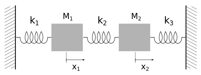
Figure 1: Diagram of the experimental set-up composed of two gliders joined by springs to each other and to the fixed ends. To minimize friction the gliders move on an air track.

The experiment is as follows: with the power supply of the air track set to maximum power, the system is moved away from the equilibrium position and the motion of the gliders is recorded by a digital camera. In this case the camera built into a Samsung Galaxy S10e smartphone was used, fixed to a support so that its optical axis was at a right angle to the track. The digital video obtained was analysed using Tracker free software [15]. This software is commonly used to record the motion of point masses in different situations, for example the bob of a pendulum [16], the trajectory of a model car [17], or more complicated systems [18] by recording the coordinates in the laboratory frame of reference in each video frame. Other capabilities of the software allow working with a set of particle systems and obtaining their centers of mass, as well as studying the relative motions between different particles of the set [19, 20]. In this work we use these capabilities to determine the center of mass of a system consisting of two coupled oscillators, as well as the coordinates of each oscillator from the point of view of the frame of reference of the other.

4 Experimental results and discussion

We determined the positions of the gliders, $x_{1}(t)$ and $x_{2}(t)$ , by means of the automatic tracking provided by the Tracker software for arbitrary initial conditions. Analysis of the video recording of the experiment gave the changes over time shown in Fig. 2. As can be seen, the motion of the gliders was complex and was not simple harmonic motion.

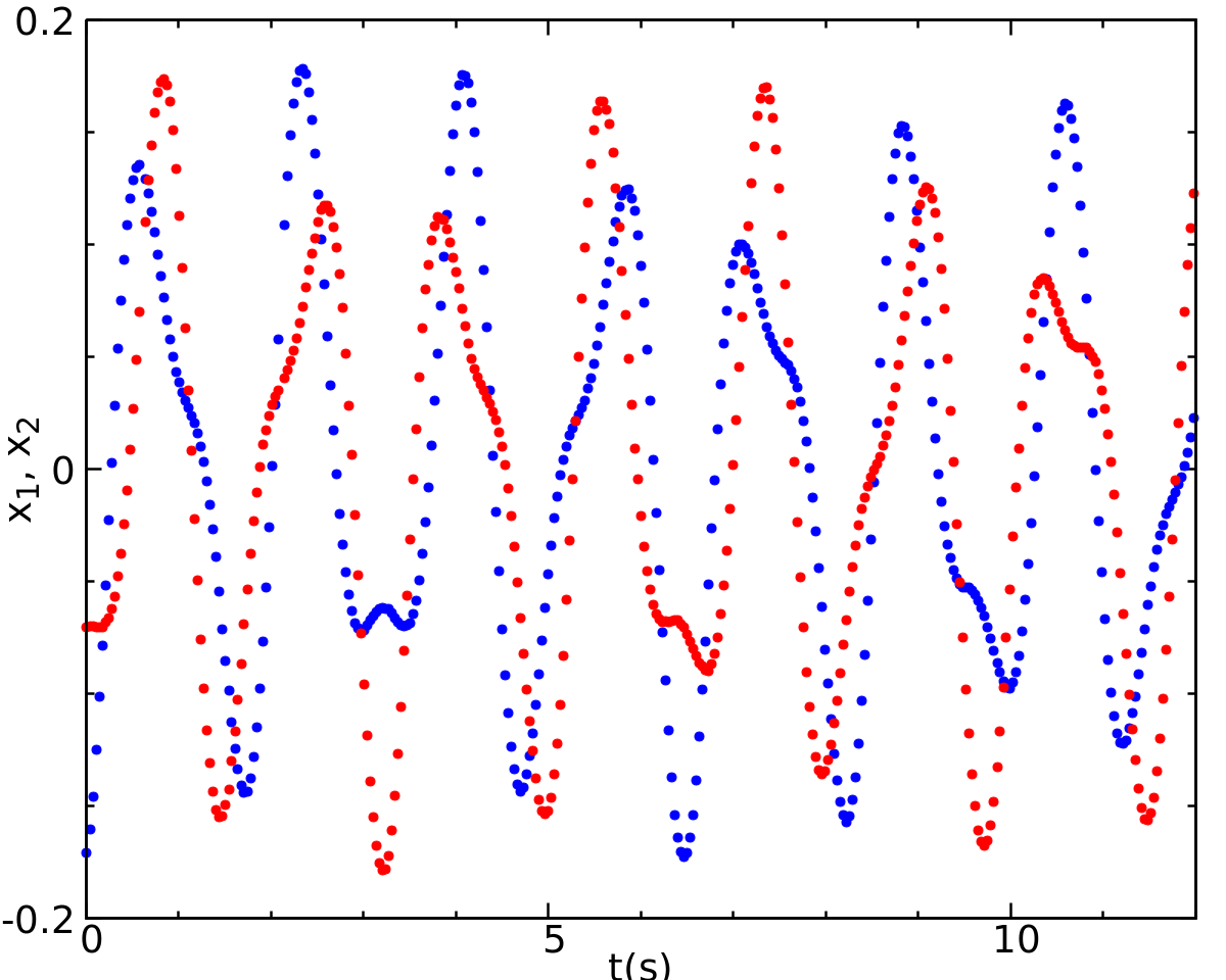
Figure 2: Temporal evolutions of the coordinates of the gliders, $x_{1}(t)$ (blue) and $x_{2}(t)$ (red), for arbitrary initial conditions.

Figure 3: Two Tracker screenshots. The top panel shows the positions of the center of mass and the symmetric coordinate $q_{S}$. The botom panel displays the relative $x_{2/1}$ and the antisymmetric $q_{A}$ coordinates (relative to the glider 1).

Afterwards, given the positions of the gliders as a function of time, using the Tracker software we determined the changes over time of the position coordinates of the center of mass of the system and of the motion of glider 2 with respect to glider 1. Figure 3 displays two screenshots of the Tracker software. Top panel illustrates the adquisition of the temporal evolution of the center of mass, $x_{cm}$ and $q_{S}$, while the bottom panel that of $x_{2/1}$ and $q_{A}$. The normal coordinates $q_{S}$ and $q_{A}$ were obtained, thanks to the Tracker, using Eqs. 5-6. It is worth noting that, as expected, $x_{cm}$ and $x_{2/1}$, proportional to the $q_{S}$ and $q_{A}$ respectively, follow a sinoudail evolution with the corresponding frequencies of the normal coordinates. It is remarkable that Tracker allows to fit the sinousoidal curves, and easily obtain the behavior or the normal coordinates. To recapitulate, the temporal evolutions of the coordinates were determined and fitted to sinusoidal functions, as shown in Fig. 4. From the parameters of the fitted curves, we obtain the normal frequencies $\omega_{S}$ and $\omega_{A}$, with their margin of uncertainty:

$$\omega_{S}=3.843(1)rad/s$$

$$\omega_{A}=6.789(1)rad/s.$$

We will refer to these frequencies as having been obtained by the normal coordinates method.

For a deeper study of the dynamics of the system, we calculated the normal frequencies by the traditional method which involves setting the initial conditions so that the gliders oscillate in the normal modes, first in symmetric and then in antisymmetric motion. We call this the normal modes method. As with the previous method, by means of video analysis we obtained the changes over time of the coordinates (not shown here) and fitted the results to sinusoidal functions. The frequencies obtained were

$$\omega_{S}=3.829(1)rad/s$$

$$\omega_{A}=6.787(1)rad/s.$$

which were slightly different from the values obtained by the normal coordinates method but always within the uncertainty margin.

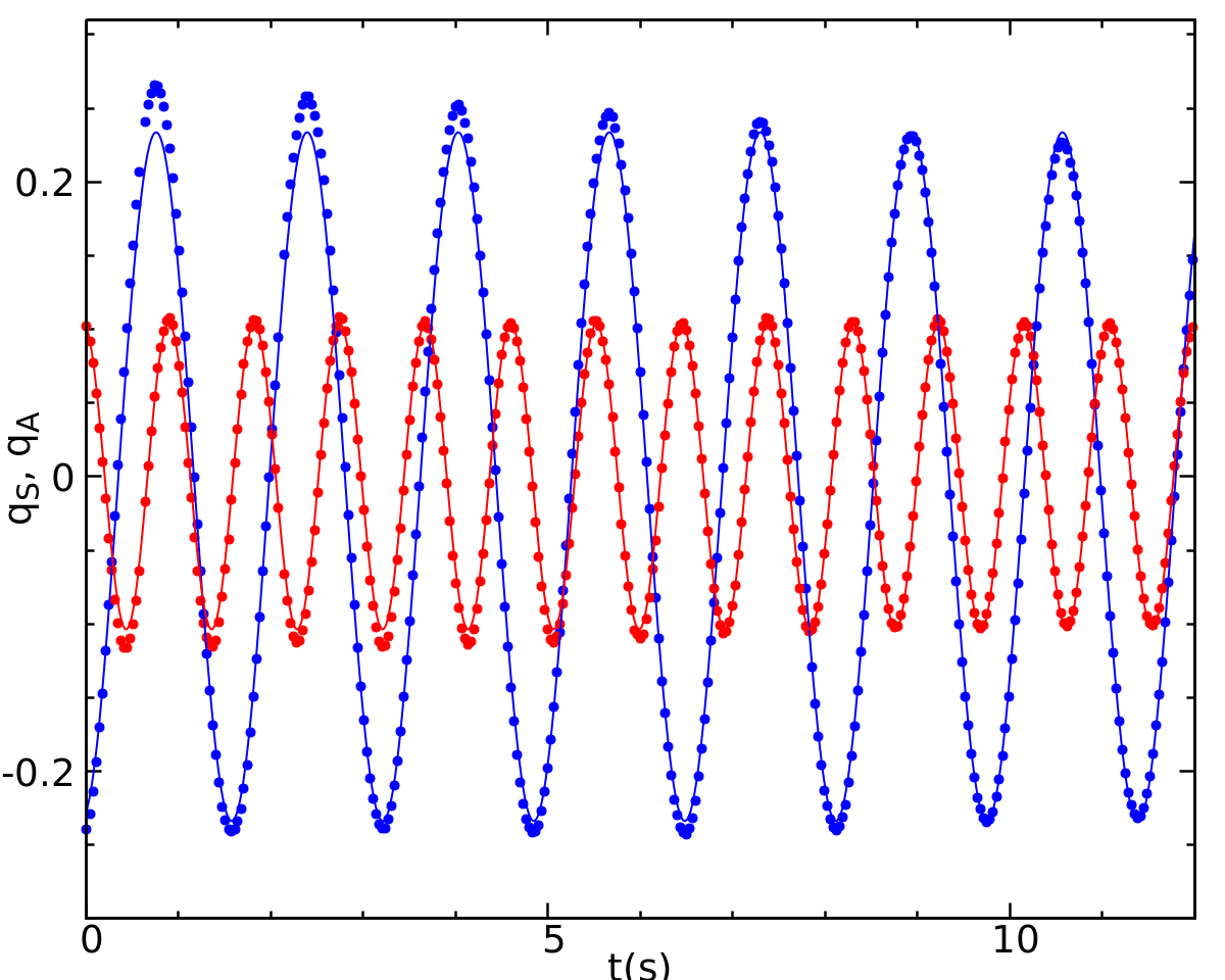
Figure 4: Temporal evolution of the normal coordinates $q_{S}$ (blue circles) and $q_{A}$ (red circles) and curves obtained by non linear fitting to sinusoidal functions (solid lines).

5 Discussion

In this section we discuss the experimental results and interpret them in the light of the results of the theoretical model. In the model presented in section 2, comprising gliders and ideal springs without mass, the results for the normal frequencies are $\omega_{S}=4.02(3)$ rad/s and $\omega_{A}=6.96(5)$ rad/s. These are different from the experimental measurements by between 2% and 5%. To analyse the causes of this discrepancy, we discuss below a model that takes into account the effect of the mass of the springs.

It is not easy to include the effect of the mass of the springs [21, 22, 23]. The pioneering work of Chen [21] begins with the hypothesis that the velocity of each spiral in a spring has a linear relationship with the distance from the fixed end. The Lagrangian of the system is developed and an overall equation for the normal frequencies of oscillation is found. In the case of a simple mass-spring system, as a first approximation the effect of the mass of the spring may be considered as a disturbance of the mass of the oscillator such that the effective mass is equal to that of the block plus one-third of the mass of the spring. This idea can be used to quantify in a simple way the effect of the mass of the springs on the normal frequencies of oscillation, when the system oscillates symmetrically and antisymmetrically, by substituting the system of coupled oscillators with an equivalent single oscillator having an elastic constant and effective mass that depend on the parameters of the system.

In the normal mode of symmetric oscillation, the central spring is not stretched, therefore the blocks of mass $M$ and the spring of mass $m$ behave as a single body of mass $2M+m$. This new body is joined on both sides to identical springs, each having elastic constant $k$ and mass $m$. Thus both springs behave as a single spring with effective elastic constant $k_{eff}=2k$ and mass $2m$. Using the approximation that $1/3$ of the mass of each spring is contributed to the total mass of the system, the effective mass of the equivalent oscillator is $M_{eff}=2M+m+2m/3$. Then the frequency of symmetric oscillation is:

$$\omega_{S}=\sqrt{\frac{k}{M+5m/6}}.$$

We can carry out a similar analysis for the normal mode of antisymmetric oscillation. In this case the midpoint of the central spring is a fixed point, so the system can be divided into two halves. Each half is composed of a spring with elastic constant $k$ and mass $m$ joined to a block of mass $M$, which in turn is joined to another spring which is half as long as the original spring, so that it has elastic constant $2k$ and mass $m/2$. This system then has an effective elastic constant $k_{eff}=k+2k$ and effective mass $M_{eff}=M+m/2$. Finally we obtain the frequency of asymmetric oscillation:

$$\omega_{A}=\sqrt{\frac{3k}{M+m/2}}.$$

Now we can compare the experimental results obtained by the methods described above, with the results of the theoretical models which depend on the spring constants and the masses of the gliders, in the case which assumes the springs have no mass, as well as the case which includes a correction for the mass of the springs. The results are compared in Table 1.

–	Normal coordinates	Theoretical model	Theoretical model	Normal modes
	method	(massless springs)	(springs with mass)	method
$\omega_{S}$	3.843(1) rad/s	4.02(3) rad/s	3.93(3) rad/s	3.829(1) rad/s
Rel. deviation	–	0.046	0.022	0.0036
$\omega_{A}$	6.789(1) rad/s	6.96(5) rad/s	6.87(6) rad/s	6.787(1) rad/s
Rel. deviation	–	0.025	0.012	0.0003

Table 1: Comparison between experimental results and models.

We can see that there is good agreement between the normal frequencies obtained by all four procedures. The small discrepancy between the experimental results may be due to the fact that it is not possible to excite only a single mode and inevitably a mixture occurs with energy transfer from one mode to the other, alternately. Comparing the experimental results with the theoretical model there is also very satisfactory agreement, especially when the correction for the mass of the springs is taken into account.

6 Conclusion

In this work we developed an experimental method which allows direct visualization of the changes over time of the normal coordinates of a system comprising two coupled oscillators with arbitrary initial conditions and studied the influence of the masses of the springs. Due to the video analysis capabilities of Tracker software it was easy to find the changes over time of the center of mass of the system and of the motion of one glider with respect to the other and afterwards of the normal coordinates. Finally we observed that the changes of the normal coordinates followed simple harmonic motion and we measured the frequencies by means of non linear fitting. We compared the results obtained by exciting each of the normal modes separately, and compared these with the predictions of theoretical models with and without correction for the mass of the springs. Agreement between the experimental results and the predictions of the theoretical models was very good in all cases. However, taking into account the mass of the springs improved considerably the agreement.

It should be noted that the ease and speed of data processing makes the activity presented here suitable not only for undergraduate laboratory courses, but also for direct analysis of the video of the experiment in theoretical classes, using for example active methodologies such as Interactive Lecture Demonstrations [24] and emphasizing activities with sequences like POE (Predict – Observe – Explain). Finally, we stress that the most significant contribution of this work is the possibility of showing the changes over time of the normal coordinates in advanced courses of mechanics and waves and allowing students to visualize their dynamics, showing that these coordinates are not just a mere mathematical contrivance for solving systems of differential equations.

References

References

- [1] Anthony Philip French. Vibrations and waves, 2001.
- [2] Frank S Crawford. Waves, berkeley physics course. 1968.
- [3] Henry SC Chen. Coupled oscillators and normal coordinates. American Journal of Physics, 35(10):924–926, 1967.
- [4] William M Wehrbein. Using video analysis to investigate intermediate concepts in classical mechanics. American Journal of Physics, 69(7):818–820, 2001.
- [5] T Greczylo and E Debowska. Using a digital video camera to examine coupled oscillations. European journal of physics, 23(4):441, 2002.
- [6] Ryan Givens, OF de Alcantara Bonfim, and Robert B Ormond. Direct observation of normal modes in coupled oscillators. American Journal of Physics, 71(1):87–90, 2003.
- [7] Juan A Monsoriu, Marcos H Giménez, Jaime Riera, and Ana Vidaurre. Measuring coupled oscillations using an automated video analysis technique based on image recognition. European journal of physics, 26(6):1149, 2005.
- [8] Juan Carlos Castro-Palacio, Luisberis Velázquez-Abad, Fernando Giménez, and Juan A Monsoriu. A quantitative analysis of coupled oscillations using mobile accelerometer sensors. European Journal of Physics, 34(3):737, 2013.
- [9] I Singh, B Kaur, and K Khun Khun. Simulating longitudinal vibrations of coupled oscillator using the fourth-order runge–kutta method by programming spreadsheet. European Journal of Physics, 40(4):045003, 2019.
- [10] T Corridoni and M D’Anna. Selective suppression of normal modes in coupled oscillators. European Journal of Physics, 41(1):015004, 2019.
- [11] Luis Tuset-Sanchis, Juan C Castro-Palacio, José A Gómez-Tejedor, Francisco J Manjón, and Juan A Monsoriu. The study of two-dimensional oscillations using a smartphone acceleration sensor: example of lissajous curves. Physics Education, 50(5):580–586, aug 2015.
- [12] Marcos H Giménez, Juan Carlos Castro-Palacio, José Antonio Gómez-Tejedor, Luisberis Velazquez, and Juan A Monsoriu. Theoretical and experimental study of the normal modes in a coupled two-dimensional system. Revista mexicana de física E, 63(2):100–106, 2017.
- [13] John R Taylor. Classical mechanics. University Science Books, 2005.
- [14] David Morin. Introduction to classical mechanics: with problems and solutions. Cambridge University Press, 2008.
- [15] Douglas Brown and Anne J Cox. Innovative uses of video analysis. The Physics Teacher, 47(3):145–150, 2009.
- [16] Martín Monteiro, Cecilia Cabeza, and Arturo C. Marti. Acceleration measurements using smartphone sensors: Dealing with the equivalence principle. Revista Brasileira de Ensino de Física, 37:1303 –, 03 2015.
- [17] Álvaro Suárez, Daniel Baccino, and Arturo C Martí. A dynamical model of remote-control model cars. Physics Education, 54(3):035007, feb 2019.
- [18] Isabel Salinas, Martin Monteiro, Arturo C Marti, and Juan A Monsoriu. Dynamics of a yoyo using a smartphone gyroscope sensor. arXiv preprint arXiv:1903.01343, 2019.
- [19] Álvaro Suárez, Daniel Baccino, and Arturo C Martí. An experiment to address conceptual difficulties in slipping and rolling problems. Physics Education, 55(1):013002, 2019.
- [20] Álvaro Suárez, Daniel Baccino, and Arturo C Martí. Video-based analysis of the transition from slipping to rolling. The Physics Teacher, 58(3):170–172, 2020.
- [21] Henry SC Chen. Note on the principal frequencies of a double spring-mass system. American Journal of Physics, 25(5):311–312, 1957.
- [22] JG Fox and J Mahanty. The effective mass of an oscillating spring. American Journal of Physics, 38(1):98–100, 1970.
- [23] Ernesto E Galloni and Mario Kohen. Influence of the mass of the spring on its static and dynamic effects. American Journal of Physics, 47(12):1076–1078, 1979.
- [24] David R Sokoloff and Ronald K Thornton. Using interactive lecture demonstrations to create an active learning environment. The Physics Teacher, 35(6):340–347, 1997.