MS-TP-20-20
Interface roughening in two dimensions

Abstract

Roughening of interfaces implies the divergence of the interface width $w$ with the system size $L$. For two-dimensional systems the divergence of $w^{2}$ is linear in $L$. In the framework of a detailed capillary wave approximation and of statistical field theory we derive an expression for the asymptotic behaviour of $w^{2}$, which differs from results in the literature. It is confirmed by Monte Carlo simulations.

1 Introduction

Roughening of interfaces in three-dimensional thermodynamical systems is a well-studied phenomenon [1, 2, 3, 4, 5, 6, 7]. A system may under suitable conditions show coexistence of two phases that are spatially separated by an interface. In a range of temperatures $T_{R}<T<T_{c}$ below the critical point, the corresponding breaking of translation invariance is associated with Goldstone modes, which manifest themselves as long-wavelength fluctuations of the interface and lead to its roughening. The most characteristic feature of interface roughening is the fact that the width of the interface increases with the size of the system. In the so-called capillary wave approximation [1, 3] the width $w$ of an interface with quadratic shape $L\times L$ is given by an integral over wave numbers $q$

$$w^{2}=\frac{1}{\sigma}\int\!\frac{d^{2}q}{(2\pi)^{2}}\,\frac{1}{q^{2}}=\frac{1}{2\pi\sigma}\int_{q_{\textrm{min}}}^{q_{\textrm{max}}}\frac{dq}{q}\qquad(d=3),$$ (1)

where $\sigma=\tau/kT$ is the reduced interface tension. The lower cutoff on wave numbers is given by $q_{\textrm{min}}=2\pi/L$. The upper cutoff represents the scale beyond which the capillary wave approximation ceases to be valid. Assuming that the lower limit on the wavelengths of capillary waves is of the order of the correlation length $\xi$, we write $q_{\textrm{max}}=1/c\,\xi$ with an adjustable numerical factor $c$. This leads to

$$w^{2}=\frac{1}{2\pi\sigma}\ln\frac{L}{2\pi c\,\xi}\qquad(d=3).$$ (2)

The special feature of this expression is the fact that the logarithmic divergence and the prefactor $1/2\pi\sigma$ are universal and do not depend on the details of the cutoffs. In particular, the expression is not affected by the fact that the proper discrete sum over wave numbers is approximated by an integral. It also does not depend on the microscopic structure of the model. In fact, a complete exact calculation in renormalised three-dimensional field theory to one-loop order without any ad hoc cutoffs [8] confirms that the large-$L$ behaviour of the interface width is given by Eq. (2). It has also been observed in a number of Monte Carlo investigations of interfaces in the three-dimensional Ising model, see [9, 10] and references therein.

In two dimensions the situation is completely different. A direct transcription of the capillary wave formula (1) to two dimensions gives

$$w^{2}=\frac{1}{\sigma}\int\!\frac{dq}{2\pi}\,\frac{1}{q^{2}}=\frac{1}{\pi\sigma}\int_{q_{\textrm{min}}}^{q_{\textrm{max}}}\frac{dq}{q^{2}}=\frac{L}{2\pi^{2}\sigma}-\frac{c\,\xi}{\pi\sigma}\qquad(d=2).$$ (3)

Here the expression for the leading linear divergence with $L$ is not universal, depending on the summation of the wave numbers as an integral and on the particular choice of the lower cutoff.

Before going into more details let us make some general remarks about interface roughening in two dimensions. In this case the “interface”, separating coexisting phases, is a one-dimensional line. The most prominent two-dimensional model, in which interfaces have been studied, is the Ising model, but other models have been studied as well with comparable results. To be definite, we shall consider the Ising model on an $L\times M$ square lattice with unit lattice spacing in the following. In the low temperature phase, an interface along the $L$-direction can be forced to be present by suitable boundary conditions. One possibility is to choose fixed positive spins on half of the boundary and negative spins on the other half. Another choice are periodic boundary conditions in the $L$-direction, and antiperiodic ones in the $M$-direction. These boundary conditions have the advantage to respect translational invariance of the system. There exist different definitions for the interface tension [11], which, however, lead to the same value [12]

$$\sigma=2\beta+\ln\tanh\beta\qquad(\beta>\beta_{c}),$$ (4)

where $\beta=1/kT$ is the inverse temperature. In addition, the interface is related to the correlation length $\xi$ by the exact identity

$$2\sigma\xi=1\,.$$ (5)

It has been shown rigorously that roughening is present for all temperatures below the critical temperature and that the leading divergence of the squared interface width $w^{2}$ with the system extent $L$ is linear [13, 14, 11]. For the form of this linear term one finds, however, different results in the literature. Gelfand and Fisher [15] discuss the capillary wave approximation with

$$w^{2}\sim\frac{L}{2\pi^{2}\sigma}$$ (6)

as in Eq. (3). Based on exact results for the Ising model, Abraham [16] and Fisher et al. [17] give

$$w^{2}\sim\frac{L}{\Gamma},$$ (7)

where

$$\Gamma=\sinh\sigma$$ (8)

can be interpreted as an effective interface tension in a generalised capillary wave approximation.

2 Theoretical Results for the Interface Width

In view of these conflicting results we shall investigate the divergence of the interface width with the system size $L$ more thoroughly. In the capillary wave approximation the interface is in the scaling region near the critical point represented by a continuous line, whose transverse elongation $h(x)$ (“height”) is Gaussian distributed with a probability distribution

$$p_{\text{CWA}}\propto\exp\left\{-\frac{\sigma}{2}\int\!dx\,\left(\frac{dh}{dx}\right)^{2}\right\}.$$ (9)

In a system of finite extent $L$ the allowed wave numbers for the height function are

$$q_{n}=\frac{2\pi}{L}n,\quad\text{with}\quad n\in\mathbf{Z},$$ (10)

and their increment is $\Delta q=\frac{2\pi}{L}$. The interface width $w$ is given by

$$w^{2}=\langle h^{2}\rangle=\frac{1}{\sigma}\sum_{q_{n}\neq 0}\frac{\Delta q}{2\pi}\frac{1}{q^{2}}.$$ (11)

The zero mode $q_{0}=0$ describes a rigid translation of the interface and has to be omitted in the sum. Furthermore we may introduce an upper cutoff of the order of the inverse correlation length

$$q_{\text{max}}=\frac{2\pi}{L}N\doteq 1/c\,\xi,$$ (12)

leading to

$$w^{2}=\frac{2}{\sigma L}\left(\frac{L}{2\pi}\right)^{2}\,\sum_{n=1}^{N}\frac{1}{n^{2}}.$$ (13)

We write the sum as

$$\sum_{n=1}^{N}\frac{1}{n^{2}}=\sum_{n=1}^{\infty}\frac{1}{n^{2}}-\sum_{n=N+1}^{\infty}\frac{1}{n^{2}}.$$ (14)

The first term is given by Euler’s solution of the Basel problem [18]:

$$\sum_{n=1}^{\infty}\frac{1}{n^{2}}=\frac{\pi^{2}}{6}.$$ (15)

The second term can be estimated by Euler’s summation formula [19]:

$$\sum_{n=N+1}^{\infty}\frac{1}{n^{2}} =\sum_{n=N}^{\infty}\frac{1}{n^{2}}-\frac{1}{N^{2}}=\int_{N}^{\infty}dx\,\frac{1}{x^{2}}+\frac{1}{2}\frac{1}{N^{2}}-\frac{1}{N^{2}}+O(N^{-3})$$ (16)

$$=\frac{1}{N}-\frac{1}{2}\frac{1}{N^{2}}+O(N^{-3}).$$ (17)

Putting things together we arrive at

$$w^{2}=\frac{1}{12\sigma}L-\frac{c\,\xi}{\pi\sigma}+O(1/L).$$ (18)

The leading large-$L$ term is clearly different from the cited predictions in Eqs. (6),(7). Its form depends on the specific infrared cutoff by taking the discreteness of the wave numbers into account.

This result can be confirmed by statistical field theory. In the scaling region the microscopic degrees of freedom are described by a real valued order parameter field $\phi(x)$, governed by a Landau-Ginzburg Hamiltonian [20]. In the two-phase region the interface is represented by an interface profile function $\phi_{R}(x)$, given by a classical solution [21, 22] plus fluctuation contributions [23, 24]. The fluctuation contributions in three dimensions have been calculated analytically in one-loop order by means of the inverse fluctuation operator in the interface background field [8]. The resulting profile function deviates from the Fisk-Widom scaling form [25] by depending logarithmically on the system size $L$. The corresponding calculation can be performed for the two-dimensional case. It is not appropriate to repeat the details of the method here. We restrict ourselves to point out that the leading large-$L$ term of the profile function, given in Eqs. (50),(52) of Ref. [8] for the three-dimensional case, contains a contribution with a factor $C_{1}$, which in two dimensions reads

$$C_{1}=\frac{3L}{32\pi^{2}\xi}\sum_{n\neq 0}\frac{1}{n^{2}}=\frac{3L}{16\pi^{2}\xi}\sum_{n=1}^{\infty}\frac{1}{n^{2}}=\frac{L}{32\,\xi}.$$ (19)

The interface width is defined through the second moment of a distribution $p(x)$,

$$w^{2}=\int\!dx\,x^{2}p(x),$$ (20)

which is defined through the derivative of the profile as in Ref. [3],

$$p(x)\propto\partial_{x}\phi_{R}(x),\qquad\int\!dx\,p(x)=1.$$ (21)

The squared width $w^{2}$ has an $L$-dependent contribution

$$\frac{8}{3\sigma}\xi C_{1}=\frac{1}{12\sigma}L$$ (22)

in exact agreement with the result (18).

The capillary wave approximation (11) can even be extended to take the discreteness of the lattice into account. If there are $L$ lattice points along the interface, the allowed wave numbers for periodic boundary conditions are given by

$$q_{n}=\frac{2\pi}{L}n,\quad\text{with}\quad n=0,1,2,\ldots,L-1.$$ (23)

The inverse Laplacean in wave number space is given by [26]

$$\frac{1}{\hat{q}_{n}^{2}}\quad\text{with}\quad\hat{q}_{n}=2\sin\frac{q_{n}}{2}.$$ (24)

The squared interface width is then given by

$$w^{2}=\frac{1}{\sigma L}\sum_{n=1}^{L-1}\frac{1}{\hat{q}_{n}^{2}}=\frac{1}{4\sigma L}\sum_{n=1}^{L-1}\frac{1}{\sin^{2}\frac{\pi n}{L}}.$$ (25)

For large $L$ the sum can be estimated with the help of Euler’s summation formula. Leaving out the details, the result is

$$\sum_{n=1}^{L-1}\frac{1}{\sin^{2}\frac{\pi n}{L}}=\frac{L^{2}}{3}+\text{const.}+O(1/L),$$ (26)

and consequently

$$w^{2}=\frac{1}{12\sigma}L+O(1/L).$$ (27)

3 Monte Carlo Simulation

In order to check the theoretical result we have performed a Monte Carlo simulation of the two-dimensional Ising model on a $L\times M$ lattice with periodic/antiperiodic boundary conditions. The lattice size has been chosen to be $M=100$ and $40\leq L\leq 200$ in steps of 10. Configurations have been generated with the Metropolis method at an inverse temperature $\beta=0.46905$ slightly above $\beta_{c}=\frac{1}{2}\ln(1+\sqrt{2})=0.44069$. The corresponding correlation length and interface tension are $\xi=4.49$ and $\sigma=0.111$. Due to the antiperiodic boundary conditions in one direction, an interface forms in the system. An example configuration is shown in Fig. 1.

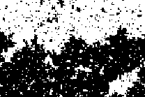
Figure 1: A configuration of Ising spins on a $150\times 100$ lattice showing an interface.

At each value of $L$ a number of thermalisation sweeps has been performed, from 5.000 at $L=40$ to 20.000 at $L=200$, followed by sweeps for the measurements. The total number of sweeps has been 700.000 for each $L$. The measured integrated autocorrelation time varies between 20 to 30 sweeps. Statistical errors have been estimated by means of the Jackknife method.

For each configuration the interface is being centered, respecting translational invariance, by means of the boundary shift method, which is explained in detail in Ref. [10]. The interface profiles are then calculated as the statistical averages of the mean magnetisation in columns of length $L$. For some values of $L$ the resulting profiles are displayed in Fig. 2.

For each obtained interface profile its squared width $w^{2}$ is calculated as the second moment of the distribution defined through the normalised derivative of the profile. Fig. 3 shows the results as a function of $L$ together with a linear fit of the form $w^{2}=aL+b$. For the coefficients we find $a=0.78\pm 0.03$ and $b=-11\pm 4$. With the present values for $\sigma$ and $\xi$, the theoretical result (18) amounts to

$$w^{2}=0.749\,L-12.9\,c.$$ (28)

The slope $a=0.78\pm 0.03$ is well consistent with the predicted value, confirming the theoretical result. The coefficient $c$ in the intercept is consistent with a value near 1.

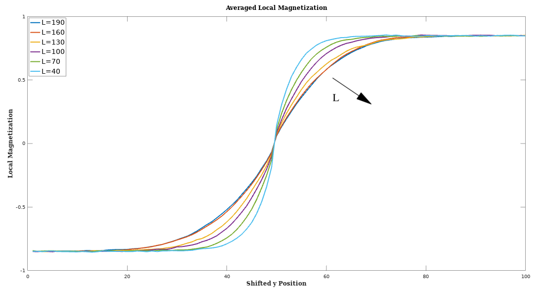
Figure 2: Numerical results for the interface profiles for some values of $L$. The broadening of the interface with increasing $L$ is clearly visible. For better visibility the numerical errors are not displayed. The errors of the widths are shown in Fig. 3.

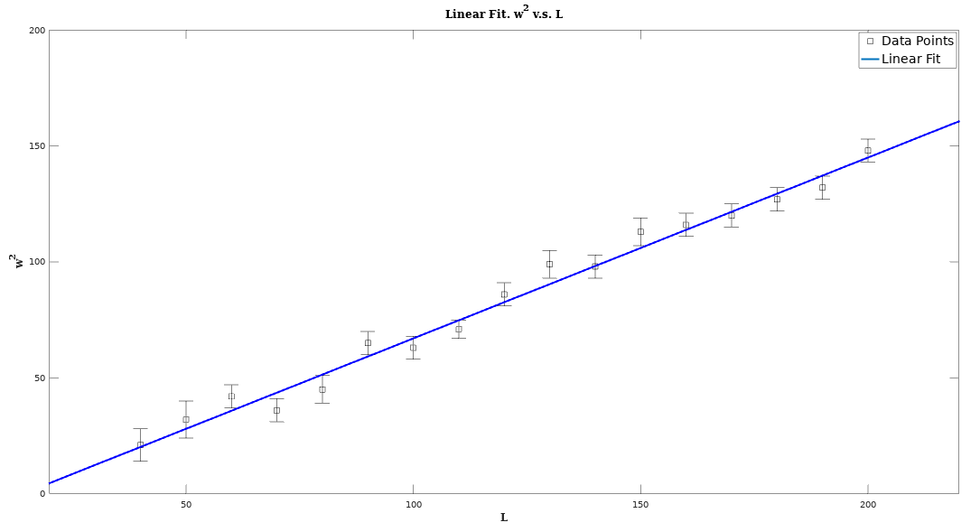
Figure 3: Squared interface widths plotted versus system size $L$, and a linear fit to the data.

4 Conclusion

The broadening of interfaces is characteristic for the roughening phenomenon. For two-dimensional systems the squared interface width diverges linearly with the system size. In contrast to the three-dimensional case, the precise form of this behaviour is not universal and does depend on the details of the model. In the framework of a detailed capillary wave approximation and of statistical field theory we have obtained a theoretical prediction for the divergence of the interface width. The result is confirmed by means of numerical simulations of the two-dimensional Ising model.

References

- [1] L. Mandelstam: Über die Rauhigkeit freier Flüssigkeitsoberflächen. Ann. Phys. 41, 609–624 (1913)
- [2] W. K. Burton and N. Cabrera: Crystal growth and surface structure. Part I. Discuss. Faraday Soc. 5, 33–39 (1949)
- [3] F. P. Buff, R. A. Lovett and F. H. Stillinger: Interfacial density profile for fluids in the critical region. Phys. Rev. Lett. 15, 621–623 (1965)
- [4] J. D. Weeks, G. H. Gilmer and H. J. Leamy: Structural transition in the Ising-model interface. Phys. Rev. Lett. 31, 549–551 (1973)
- [5] J. D. Weeks: Structure and thermodynamics of the liquid–vapor interface. J. Chem. Phys. 67, 3106–3121 (1977)
- [6] J. Rowlinson and B. Widom: Molecular Theory of Capillarity. Clarendon Press, Oxford (1982)
- [7] D. Jasnow: Critical phenomena at interfaces. Rep. Prog. Phys. 47, 1059–1132 (1984)
- [8] M. H. Köpf and G. Münster: Interfacial roughening in field theory. J. Stat. Phys. 132, 417–430 (2008)
- [9] A. Werner, F. Schmid, M. Müller and K. Binder: “Intrinsic” profiles and capillary waves at homopolymer interfaces: A Monte Carlo study. Phys. Rev. E 59, 728–738 (1999)
- [10] M. Müller and G. Münster: Profile and width of rough interfaces. J. Stat. Phys. 118, 669–686 (2005)
- [11] D. B. Abraham: Surface structures and phase transitions - exact results, in Phase Transitions and Critical Phenomena, Vol. 10, C. Domb and J. L. Lebowitz (eds.). Academic Press, London (1986)
- [12] L. Onsager: Crystal statistics I. Phys. Rev. 65, 117–149 (1944)
- [13] G. Gallavotti: The phase separation line in the two-dimensional Ising model. Commun. Math. Phys. 27, 103–136 (1972)
- [14] D. B. Abraham and P. Reed: Phase separation in the two-dimensional Ising ferromagnet. Phys. Rev. Lett. 33, 377–379 (1974)
- [15] M. P. Gelfand and M. E. Fisher: Finite size effects in fluid interfaces. Physica A 166, 1–74 (1990)
- [16] D. B. Abraham: Capillary waves and surface tension: an exactly solvable model. Phys. Rev. Lett. 47, 545–548 (1981)
- [17] M. P. A. Fisher, D. S. Fisher and J. D. Weeks: Agreement of capillary-wave theory with exact results for the interface profile of the two-dimensional Ising model. Phys. Rev. Lett. 48, 368 (1982)
- [18] L. Euler: De summis serierum reciprocarum. Commentarii academiae scientiarum Petropolitanae 7, 123–134 (1740)
- [19] L. Euler: Methodus generalis summandi progressiones. Commentarii academiae scientiarum Petropolitanae 6, 68–97 (1738)
- [20] M. Le Bellac: Quantum and Statistical Field Theory. Clarendon Press, Oxford (1991)
- [21] J. van der Waals: Thermodynamische theorie der capillariteit in de onderstelling van continue dichtheidsverandering. Verhandel. Konink. Akad. Weten. Amsterdam 1 (1893) (in Dutch). English translation: J. Rowlinson: The thermodynamic theory of capillarity under the hypothesis of a continuous variation of density. J. Stat. Phys. 20, 197–244 (1979)
- [22] J. W. Cahn and J. E. Hilliard: Free energy of a nonuniform system. I. Interfacial free energy. J. Chem. Phys. 28, 258–267 (1958)
- [23] D. Jasnow and J. Rudnick: Interfacial profile in three dimensions. Phys. Rev. Lett. 41, 698–701 (1978)
- [24] G. Münster: Interface tension in three-dimensional systems from field theory. Nucl. Phys. B 340, 559–567 (1990)
- [25] S. Fisk and B. Widom: Structure and free energy of the interface between fluid phases in equilibrium near the critical point. J. Chem. Phys. 50, 3219–3227 (1960)
- [26] I. Montvay and G. Münster: Quantum Fields on a Lattice. Cambridge University Press (1994)