Description of the low-lying collective states of ⁹⁶Zr based on the quadrupole-collective Bohr Hamiltonian

Abstract

Background:

Experimental data on ⁹⁶Zr indicate coexisting spherical and deformed structures with small mixing amplitudes. Several collective low-lying states and E2 and M1 transitions are observed for this nucleus. A consideration of these data in the full framework of the Geometrical Collective Model is necessary for ⁹⁶Zr.

Purpose:

To investigate the observed properties of the low-lying collective states of ⁹⁶Zr based on the Geometrical Collective Model.

Method:

The quadrupole-collective Bohr Hamiltonian depending on both $\beta$ and $\gamma$ shape variables with a potential having spherical and deformed minima, is applied. The relative depth of two minima, height and width of the barrier, rigidity of the potential near both minima are determined so as to achieve a satisfactory description of the observed properties of the low-lying collective quadrupole states of ⁹⁶Zr.

Results:

Good agreement with the experimental data on the excitation energies, $B(E2)$ and $B(M1;2^{+}_{2}\rightarrow 2^{+}_{1})$ reduced transition probabilities is obtained.

Conclusion:

It is shown that the low-energy structure of ⁹⁶Zr can be described in a satisfactory way within the Geometrical Collective Model with a potential function supporting shape coexistence without other restrictions of its shape. However, the excitation energy of the $2^{+}_{2}$ state can be reproduced only if the rotation inertia coefficient is taken by four times smaller than the vibrational one in the region of the deformed well. It is shown also that shell effects are important for the description of the $B(M1;2^{+}_{2}\rightarrow 2^{+}_{1})$ and $B(M1;3^{+}_{1}\rightarrow 2^{+}_{1})$ transition probabilities. An indication for the influence of the pairing vibrational mode on the $0^{+}_{2}\rightarrow 0^{+}_{1}$ transition is confirmed in agreement with the previous result.

I Introduction

It is well known for a long time that nuclei can exhibit both spherical and deformed shapes including the intermediate region of nuclei transitional from spherical to deformed. What is more interesting is the phenomenon that a given nucleus can exhibit different shapes depending on the excitation energy. This phenomenon of shape coexistence has in recent years become the subject of many investigations in nuclear physics. Even more, shape coexistence is becoming to be considered a near-universal property of nuclei Heyde1 . A large number of papers, including reviews Heyde1 ; Heyde2 ; Heyde3 ; Poves , are devoted to investigation of shape coexistence Garcia ; Togashi ; Gavrilov ; Sieja ; Garcia2 ; Boyukata ; Liu ; Petrovici1 ; Rodriguez ; Skalski1 ; Xiang ; Mei ; Skalski2 ; Ozen ; Fortune ; Buscher . Various approaches have been employed to study this phenomenon Bender ; Niksic ; Federman ; Heyde4 ; Etch ; Holt ; Niksic1 .

Among different examples of shape coexistence evidence for Zr isotopes with their change of the shape with excitation energy are especially interesting. Shape evolution can be characterized by a smooth or abrupt transition from spherical to deformed shape, and a significant or suppressed mixing of configurations with different shapes can take place. Such information is contained in electromagnetic transition probabilities and a high purity of coexisting shapes has been established in ⁹⁶Zr Kremer .

In this paper we apply the Geometrical Collective-quadrupole Model to a description of the properties of the low-lying states of ⁹⁶Zr including the shape coexistence phenomenon. Although an explanation of shape coexistence is a subject of microscopic nuclear modeling the Geometrical Collective Model deals directly with shape dynamical variables and, thus, may be capable of describing the dynamical consequences of shape coexistence and the properties of the collective low-lying states in general.

It is an open question whether a potential function in terms of shape variables can exist which allows for a reproduction of the data on the coexisting quadrupole collective structures of ⁹⁶Zr. The aim of the present paper is to investigate a possibility to describe, in principle, the properties of the low-lying collective states of ⁹⁶Zr and the amount of mixing of the configurations characterized by spherical and deformed shapes based on the quadrupole collective Bohr Hamiltonian. It is also interesting in what characteristics of the collective states shell effects are most pronounced.

II Hamiltonian

The quadrupole-collective Bohr Hamiltonian can be written as Niksic2

$$H = -\frac{\hbar^{2}}{2\sqrt{\omega r}}\left(\frac{1}{\beta^{4}}\left[\frac{\partial}{\partial\beta}\sqrt{\frac{r}{\omega}}\beta^{4}B_{\gamma\gamma}\frac{\partial}{\partial\beta}-\frac{\partial}{\partial\beta}\sqrt{\frac{r}{\omega}}\beta^{3}B_{\beta\gamma}\frac{\partial}{\partial\gamma}\right]\right.$$ (1)

$$+ \left.\frac{1}{\beta\sin{3\gamma}}\left[-\frac{\partial}{\partial\gamma}\sqrt{\frac{r}{\omega}}\sin{3\gamma}B_{\beta\gamma}\frac{\partial}{\partial\beta}+\frac{1}{\beta}\frac{\partial}{\partial\gamma}\sqrt{\frac{r}{\omega}}\sin{3\gamma}B_{\beta\beta}\frac{\partial}{\partial\gamma}\right]\right)$$

$$+ \frac{1}{2}\sum_{k=1}^{3}\frac{\hat{J}^{2}_{k}}{\Im_{k}(\beta)}+V(\beta,\gamma),$$

where $\omega=B_{\beta\beta}B_{\gamma\gamma}-B^{2}_{\beta\gamma}$ is the determinant of the vibrational inertia tensor

$$B_{vib}=\begin{pmatrix}B_{\beta\beta}&\beta B_{\beta\gamma}\\ \beta B_{\beta\gamma}&\beta^{2}B_{\gamma\gamma}\end{pmatrix}.$$ (2)

The moments of inertia $\Im_{k}$ with respect to the body-fixed axes are expressed as

$$\Im_{k}=4B_{k}(\beta)\beta^{2}\sin^{2}{\left(\gamma-\frac{2\pi k}{3}\right)}$$ (3)

and $r=B_{1}B_{2}B_{3}$. The components of the angular momentum in the body-fixed frame are denoted as $\hat{J}_{k}$ and can be expressed in terms of the Euler angles. The potential energy is denoted as $V(\beta,\gamma)$. The Hamiltonian of Eq. (1) is a general case of the conventional Bohr Hamiltonian Bohr1952 allowing for non-diagonal vibrational inertia.

In the present work we aim to investigate whether it is possible to construct a potential energy in such a way that all existing data on the energies of the lowest angular momentum excited states and the transitions between these states will be described. If such a potential can be constructed will it demonstrate the shape coexistence by having two minima: spherical and deformed. Previously in Ref. Sazonov , this problem was solved under the assumption that the $\gamma$ degrees of freedom can be separated from $\beta$ in the potential and the value of $\gamma$ is stabilized around $\gamma=0^{\circ}$. This is obviously a rather crude approximation at least in the region of small values of $\beta$. In the present paper we avoid this assumption.

To simplify consideration, we make the following assumptions for the inertia coefficients:

$$B_{\beta\beta}=B_{\gamma\gamma}=B_{0},\hskip 10.0ptB_{\beta\gamma}=0,$$

$$B_{1}(\beta)=B_{2}(\beta)=B_{3}(\beta)=b_{rot}(\beta)B_{0},$$ (4)

where $B_{0}$ is the parameter scaling vibrational and rotational masses. We keep in Eq. (II) the rotational inertia coefficient because in the case of the well-deformed axially symmetric nuclei the inertia coefficient for the rotational motion is 4-10 times smaller than the inertia coefficient for the vibrational motion Jolos1 ; Jolos2 . In a complete correspondence with this result it is shown below that in order to explain the excitation energy of the 2${}^{+}_{2}$ state it is necessary to take $b_{rot}$ several times less than unity.

Under the assumptions of Eq. (II), the Hamiltonian (1) takes the form:

$$\hat{H} = -\frac{\hbar^{2}}{2B_{0}}\left(\frac{1}{b_{rot}^{3/2}}\frac{1}{\beta^{4}}\frac{\partial}{\partial\beta}\beta^{4}b_{rot}^{3/2}\frac{\partial}{\partial\beta}+\frac{1}{\beta^{2}\sin{3\gamma}}\frac{\partial}{\partial\gamma}\sin{3\gamma}\right)$$ (5)

$$+ \frac{1}{2}\sum_{k=1}^{3}\frac{\hat{J}^{2}_{k}}{\Im_{k}(\beta)}+V(\beta,\gamma).$$

The potential energy $V(\beta,\gamma)$ is assumed to have two minima, spherical and deformed, separated by a barrier. This is in correspondence with the considerations Garcia ; Gavrilov in the interacting boson model with configuration mixing (IBM-CM) where two configurations with different total number of bosons have been taken into account in order to include the effect of shape coexistence. We expect that the wave function of the lowest excited states are localized in these minima while the weight of the function inside the barrier region is strongly suppressed. Therefore, it is reasonable to assume that the quantity $b_{rot}$ has constant (but different) values in the regions of the spherical and deformed minima and the change from one value to another takes place in the region of the barrier. In this case, $b_{rot}$ can be taken outside of the derivative in Eq. (5) as it only gives the non-zero contribution in the barrier region where the wave function is close to zero. Thus, we obtain finally the following model Hamiltonian:

$$H = -\frac{\hbar^{2}}{2B_{0}}\left(\frac{1}{\beta^{4}}\frac{\partial}{\partial\beta}\beta^{4}\frac{\partial}{\partial\beta}+\frac{1}{\beta^{2}\sin{3\gamma}}\frac{\partial}{\partial\gamma}\sin{3\gamma}\frac{\partial}{\partial\gamma}\right.$$ (6)

$$+ \left.\sum_{k=1}^{3}\frac{\hat{J}^{2}_{k}}{4b_{rot}\beta^{2}\sin{\left(\gamma-\frac{2\pi k}{3}\right)}}\right)+V(\beta,\gamma),$$

where

$$b_{rot}=\begin{cases}1&\text{if $\beta\leq\beta_{m}$, }\\ b_{def}<1&\text{if $\beta>\beta_{m}$.}\end{cases}$$ (7)

The magnitude of the $b_{rot}$ inside the deformed minimum is obtained by fitting the excitation energy of the $2^{+}_{2}$ state. The change from the spherical to deformed value of $b_{rot}$ occurs at $\beta=\beta_{m}$ which is taken around the maximum of the barrier separating spherical and deformed potential wells. Our calculations show that the precise value of $\beta_{m}$ does not affect the qualitative results of the calculations.

To solve the eigenvalue problem with the Hamiltonian (6) we expand the eigenfunctions in terms of a complete set of basis functions that depend on the deformation variables $\beta$ and $\gamma$ and the Euler angles. For each value of angular momentum $I$, the basis functions are written as

$$\Psi_{IM}^{n_{\beta}v\alpha}=R^{(n_{\beta},v)}(\beta)\Upsilon_{v\alpha IM}(\gamma,\Omega),$$ (8)

where $\Upsilon_{v\alpha IM}$ is the SO(5)$\supset$ SO(3) spherical harmonics, which are the eigenfunctions of the operator $\hat{\Lambda}^{2}$:

$$\hat{\Lambda}^{2}\Upsilon_{v\alpha IM}=\left[-\frac{1}{\sin{3\gamma}}\frac{\partial}{\partial\gamma}\sin{3\gamma}\frac{\partial}{\partial\gamma}+\frac{1}{4}\sum_{k}\frac{\hat{J}_{k}^{2}}{\sin^{2}{(\gamma-\frac{2\pi k}{3})}}\right]\Upsilon_{v\alpha IM}=v(v+3)\Upsilon_{v\alpha IM}.$$ (9)

In addition to the angular momentum $I$ and its projection $M$, each function $\Upsilon_{v\alpha IM}$ is labeled by the SO(5) seniority quantum number $v$ and a multiplicity index $\alpha$, which is required for $v\geq 6$. In the following, both indices $v$ and $\alpha$ will be replaced by the running index $n_{\gamma}=0,1,2,\dots$.

The $\Upsilon_{v\alpha IM}$ can be explicitly constructed as a sum over the states with explicit value of the projection $K$ of the angular momentum on the intrinsic axis Rowe2004 ; Caprio2009

$$\Upsilon_{v\alpha IM}(\gamma,\Omega)=\sum_{K=0,even}^{I}F_{v\alpha I,K}(\gamma)\xi_{KM}^{I}(\Omega),$$ (10)

where

$$\xi_{KM}^{I}(\Omega)=\frac{1}{\sqrt{2(1+\delta_{K0})}}\left[D^{I}_{M\ K}(\Omega)\right.$$ (11)

$$\left.+(-1)^{I}D^{I}_{M\ -K}(\Omega)\right]$$ (12)

and the $F_{v\alpha I,K}(\gamma)$ are polynomials constructed from the trigonometrical functions of $\gamma$ Rowe-Wood .

The basis wave functions $R^{(n_{\beta},v)}$ are chosen as the eigenfunctions of the harmonic oscillator Hamiltonian in $\beta$:

$$h_{h.o.}=\frac{1}{2}\left(-\frac{1}{\beta^{4}}\frac{\partial}{\partial\beta}\beta^{4}\frac{\partial}{\partial\beta}+\frac{v(v+3)}{\beta^{2}}+\frac{\beta^{2}}{\beta_{0}^{4}}\right).$$ (13)

The eigenfunctions of $h_{h.o.}$ have the following analytical form

$$R_{n_{\beta},v}(\beta)=N_{\beta}\left(\frac{\beta}{\beta_{0}}\right)^{v}L_{n_{\beta}}^{v+3/2}\left(\frac{\beta^{2}}{\beta_{0}^{2}}\right)\exp{\left(-\frac{\beta^{2}}{2\beta_{0}^{2}}\right)},$$ (14)

where $\beta_{0}$ is an oscillator length and the normalization constant $N_{\beta}$ is given as:

$$N_{\beta}=\sqrt{\frac{2n_{\beta}!}{\Gamma(n_{\beta}+v+5/2)}}.$$ (15)

The basis functions $R_{n_{\beta},v}$ are completely specified by the choice of the oscillator length $\beta_{0}$. Our calculations have shown that the fastest convergence of the results is obtained when $\beta_{0}$ is chosen to be equal to the value at the region of the barrier separating spherical and deformed minima so that the oscillator potential coincides with the potential $V(\beta,\gamma=0)$ at the top of the barrier. For such a choice of $\beta_{0}$, $(n_{\beta})_{max}=30$ is enough to provide a convergence.

Diagonalization of the Hamiltonian (6) is realized in the basis of SO(5)-SO(3) spherical harmonics $\Upsilon_{v\alpha IM}(\gamma,\Omega)$ truncated to some maximum seniority $v_{max}.$ As shown in Caprio2011 , taking $v_{max}=50$ is sufficient to provide a convergence of the calculation. A concrete realization of the construction of $\Upsilon_{v\alpha IM}(\gamma,\Omega)$ performed in Rowe2004 ; Caprio2009 is used in the present work. These functions were first constructed in analytic form in Bes1959 for $I\leq 6$.

The potential energy $V(\beta,\gamma)$ in (6) is chosen in the form

$$V(\beta,\gamma)=U(\beta)+C_{\gamma}\beta^{3}(1-\cos{3\gamma}).$$ (16)

In (16), the deformed minimum of the potential energy is localized around $\gamma=0$ for positive $C_{\gamma}$ as it was assumed in our previous paper Sazonov . At the same time, this form of $\gamma$-dependence of $V(\beta,\gamma)$ provides very weak $\gamma$-dependence of $V(\beta,\gamma)$ at small $\beta$ because of the factor $\beta^{3}$. The form of the potential energy at $\gamma=0$ ($U(\beta)$) and the parameter $C_{\gamma}$ which determines the stiffness of the potential with respect to $\gamma$ in the deformed minimum are fitted to reproduce the experimental data. As the first step, we have taken $U(\beta)$ as it was numerically determined in Sazonov , $B_{0}$=0.004 MeV^-1 and $b_{rot}=0.2$ and performed calculations with different values of $C_{\gamma}$. We have found that $C_{\gamma}$=50 MeV produces a reasonable value of the frequency of $\gamma$-vibrations close to 1.5 MeV. No significant changes were found in the calculation results for the excitation energies and the E2 transition probabilities when $C_{\gamma}$ was varied around 50 MeV.

As before in Sazonov , to describe the shape of the axially-symmetric part of the potential we defined several points fixing the positions of the spherical and deformed minima, the rigidity of the potential near its minima, and the height and width of the barrier separating two minima. The deformation at the second minimum has been taken to be $\beta=$ 0.24 in agreement with the experimental value of $B(E2;2^{+}_{2}\rightarrow 0^{+}_{2})$. The potential energy as a function of $\beta$ is determined by using a spline interpolation between selected points. Then we solve numerically the Schrödinger equation with Hamiltonian (6), varying positions of the selected points in order to get a satisfactory description of the energies of the $2^{+}_{1}$ and $2^{+}_{2}$ states and the following transition probabilities: $B(E2;2^{+}_{2}\rightarrow 0^{+}_{2})$, $B(E2;2^{+}_{1}\rightarrow 0^{+}_{1})$, and $B(E2;2^{+}_{2}\rightarrow 0^{+}_{1})$. The number of points is taken to be 16 to provide a smooth change of the potential. However, not all the points are of the same physical importance. In principle, the number of points can be minimized as, obviously, the only relative depths of the minima and the height and width of the barrier leads to physically meaningful changes. The mass parameter has been taken finally as $B_{0}=0.005$ MeV^-1 to fix the energy of the $0^{+}_{2}$ state.

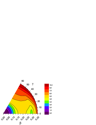
Figure 1: Potential energy $V(\beta,\gamma)$ obtained in the calculations.

The resulting potentials $V(\beta,\gamma)$ is presented in Fig. 1. It is interesting that the inclusion of $\gamma$ as a dynamical variable leads to a significant change of the shape of the potential in comparison to the case when $\gamma$ was treated as a constant and not as a variable. The most important change occurs at the region of small $\beta$ where the potential becomes shallower. In this region, the resulting potential is practically independent on $\gamma$ and the wave function of the $0^{+}_{1}$ state becomes independent on $\gamma$ as well. This is not the case if $\gamma$ is treated as a constant. This lack of the phase space results in the necessity to take a much deeper potential at small values of $\beta$ to hold the wave function of $0^{+}_{1}$ state inside the spherical minimum when $\gamma$ is not considered dynamic.

III Results

The Hamiltonian eigenfunctions $\Psi_{InM}$, where $I$ is the angular momentum, $M$ is its projection and $n$ is a multiplicity index, are obtained in calculations as a series expansions in the basic functions (8). However, for discussions below it is more convenient to present them in the basis of functions $\xi^{I}_{KM}$ (11):

$$\Psi_{InM}=\sum_{K}\psi_{InK}(\beta,\gamma)\frac{1}{\sqrt{2(1+\delta_{K0})}}\left(D^{I}_{MK}(\Omega)\right.$$

$$\left.+(-1)^{I}D^{I}_{M-K}(\Omega)\right)$$ (17)

We are using below the one-dimensional probability distributions over $\beta$ which are obtained by integration of $|\Psi_{InM}|^{2}$ over $\gamma$ and Euler angles

$$\Phi_{In}(\beta)=\beta^{4}\int_{0}^{\pi/3}\sin{3\gamma}d\gamma\int d\Omega|\Psi_{InM}|^{2}.$$ (18)

and the weights of the wave functions in the spherical minimum $W_{In}$ determined as

$$W_{In}=\int_{0}^{\beta_{m}}d\beta\Phi_{In}(\beta),$$ (19)

where $\beta_{m}$ is the position of the maximum of the barrier for $\gamma=0$.

The calculated wave function of the $0^{+}_{1}$ and $0^{+}_{2}$ states multiplied by the $\beta$ and $\gamma$- dependent volume element are presented in Fig. 2. As it is seen, the wave function of the $0^{+}_{1}$ is strongly localized in the spherical minimum. The wave function of the $0^{+}_{2}$ state is mainly localized in the deformed minimum.

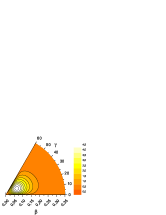
a) b)

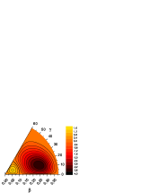
Figure 2: Wave function of the $0^{+}_{1}$ (a) and $0^{+}_{2}$ (b) states.

Their spherical weights are $W_{0_{1}}$=0.985 and $W_{0_{2}}$=0.136 for $0^{+}_{1}$ and $0^{+}_{2}$ states, respectively. The one-dimensional probability distribution over $\beta$ which can be obtained by integrating $|\Psi_{IM}^{n_{\beta}v\alpha}|^{2}$ over $\gamma$ and the Euler angles are presented in Fig. 3 for the $0^{+}_{1}$ and $0^{+}_{2}$ states.

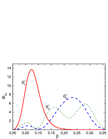
Figure 3: Distribution over $\beta$ of the squares of the wave functions of the $0^{+}_{1}$ (solid line), $0^{+}_{2}$ (dashed line) and $0^{+}_{3}$ (dotted line) states calculated according (18).

For the lowest 2⁺ states the situation is similar. The $2^{+}_{1}$ state is localized in the spherical minimum with the weight $W(2^{+}_{1})$=0.928, while the second excited $2^{+}$ state is only weakly presented there with $W(2^{+}_{2})$ =0.144.

The wave functions of the $2^{+}$ states have components with $K$=0 and $K$=2 determined by the expansion (III). The functions $\psi_{2^{+}nK}$ for $K$=0 and $K$=2 multiplied by the volume element are presented in Fig. 4 for the $2^{+}_{1}$ state and in Fig. 5 for the $2^{+}_{2}$ state.

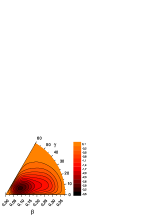
a) b)

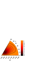
Figure 4: The components of the wave function of the $2^{+}_{1}$ state with $K=0$ (a) and $K=2$ (b) multiplied by the volume element.

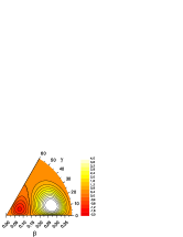
a) b)

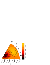
Figure 5: The components of the wave function of the $2^{+}_{2}$ state with $K=0$ (a) and $K=2$ (b) multiplied by the volume element.

Using these wave functions the matrix elements of an arbitrary operator $\hat{F}$ can be calculated as

$$<f|\hat{F}|i>=\int_{0}^{\infty}\beta^{4}d\beta\int_{0}^{\pi/3}\sin{3\gamma}d\gamma\int d\Omega\Psi_{f}^{*}\hat{F}\Psi_{i}.$$ (20)

We are particularly interested in calculations of the $E2$ and $M1$ transition probabilities. The collective quadrupole operator responsible for $E2$ transitions is taken in the form

$$Q^{coll}_{2\mu} = \frac{3Ze}{4\pi}R_{0}^{2}\left(\beta\cos{\gamma}\phantom{\frac{1}{1}}\!\!\!D^{2}_{\mu 0}(\Omega)\right.$$ (21)

$$+ \left.\frac{1}{\sqrt{2}}\beta\sin{\gamma}\left(D^{2}_{\mu 2}(\Omega)+D^{2}_{\mu-2}(\Omega)\right)\right),$$

where $R_{0}$ is the equivalent volume-conserving spherical radius of the nucleus and $Z$ is the nuclear charge number. The E0 transition strength $\rho^{2}(0^{+}_{2}\rightarrow 0^{+}_{1})$ is calculated using the expression

$$\rho^{2}(0^{+}_{2}\rightarrow 0^{+}_{1})=\left(\frac{3Ze}{4\pi}\right)^{2}|\langle 0^{+}_{2}|\beta^{2}|0^{+}_{1}\rangle|^{2}$$ (22)

For the $M1$ transition operator we use the same expression as in Sazonov

$$(M1)_{\mu}=\mu_{N}\sqrt{\frac{3}{4\pi}}g_{R}(\beta)I_{\mu},$$ (23)

where $\mu_{N}$ is the nuclear magneton and $g_{R}(\beta)$ is the deformation-dependent collective $g$ factor.

The results of calculations for the energies of the low-lying states and the electromagnetic transition probabilities are presented in Table 1 and Table 2 together with the available experimental data.

Table 1: The calculated and the experimental energies of the low-lying 0⁺, 2⁺, 3⁺ and 4⁺ states. The experimental data are taken from Garcia ; nndc1

. State $E_{calc}$ (MeV) $E_{exp}$ (MeV) $E(0^{+}_{2})$ 1.582 1.582 $E(0^{+}_{3})$ 2.443 2.695 $E(0^{+}_{4})$ 3.049 2.926 $E(2^{+}_{1})$ 1.724 1.750 $E(2^{+}_{2})$ 2.236 2.226 $E(2^{+}_{3})$ 2.974 2.669 $E(2^{+}_{4})$ 3.338 3.249 $E(3^{+}_{1})$ 2.653 2.439 $E(4^{+}_{1})$ 2.983 2.857 $E(4^{+}_{2})$ 3.447 3.082

Table 2: The calculated and the experimental values of the electromagnetic transition probabilities in ⁹⁶Zr. B(E2) values are given in W.u., B(M1) - in nuclear magnetons. The value of $Q(2^{+}_{2})$ is given in $e\cdot barn$. Experimental data are taken from nndc1 ; Witt .

transitions	calc	exp
$B(E2;2^{+}_{1}\rightarrow 0^{+}_{1})$	5.23	2.3(3)
$B(E2;2^{+}_{2}\rightarrow 0^{+}_{1})$	0.39	0.26(8)
$B(E2;2^{+}_{2}\rightarrow 0^{+}_{2})$	26.0	36(11)
$B(E2;2^{+}_{2}\rightarrow 2^{+}_{1})$	6.49	2.8${}_{-1.0}^{+1.5}$
$B(E2;3^{+}_{1}\rightarrow 2^{+}_{1})$	0.22	0.1${}_{-0.1}^{+0.3}$
$B(E2;3^{+}_{1}\rightarrow 2^{+}_{2})$	4.26	-
$B(E2;0^{+}_{3}\rightarrow 2^{+}_{1})$	1.14	-
$B(E2;0^{+}_{3}\rightarrow 2^{+}_{2})$	69.8	34(9)
$B(E2;2^{+}_{3}\rightarrow 2^{+}_{1})$	10.6	50(70)
$B(E2;2^{+}_{3}\rightarrow 2^{+}_{2})$	1.85	$<400$
$B(E2;4^{+}_{1}\rightarrow 2^{+}_{1})$	16.7	16${}_{-13}^{+5}$
$B(E2;4^{+}_{1}\rightarrow 2^{+}_{2})$	43.0	56(44)
$B(E2;4^{+}_{1}\rightarrow 3^{+}_{1})$	7.59	-
$B(E2;0^{+}_{4}\rightarrow 2^{+}_{1})$	0.36	0.3(3)
$B(E2;0^{+}_{4}\rightarrow 2^{+}_{2})$	2.02	1.8(14)
$B(E2;4^{+}_{2}\rightarrow 2^{+}_{1})$	4.82	-
$B(E2;4^{+}_{2}\rightarrow 2^{+}_{2})$	16.6	-
$B(E2;4^{+}_{2}\rightarrow 3^{+}_{1})$	0.07	-
$B(E2;2^{+}_{4}\rightarrow 2^{+}_{1})$	2.53	-
$\rho^{2}(0^{+}_{2}\rightarrow 0^{+}_{1})$	0.0023	0.0075
$\rho^{2}(0^{+}_{3}\rightarrow 0^{+}_{1})$	0.001	0.004
$\rho^{2}(0^{+}_{3}\rightarrow 0^{+}_{2})$	0.038	0.0035
$B(M1;2^{+}_{2}\rightarrow 2^{+}_{1})$	0.071	0.14(5)
$B(M1;3^{+}_{1}\rightarrow 2^{+}_{1})$	0.0002	0.3(1)
$Q(2^{+}_{2})$	$-0.5$	-

As it is seen from the results presented in Tables 1 and 2 the agreement between the calculated results and the experimental data is quite satisfactory. This applies not only to the $0^{+}_{2}$, $2^{+}_{1}$ and $2^{+}_{2}$ states on which attention was focused primarily in determining the form of the collective potential.

Let us consider the results for the $0^{+}_{3}$, $0^{+}_{4}$, $2^{+}_{3}$ and $4^{+}_{1}$ excited states. The calculated energy of the $2^{+}_{3}$ state exceeds the experimental value by 300 keV which is 10% of the total excitation energy of this state. The calculated value of B(E2; $2^{+}_{3}\rightarrow 2^{+}_{1}$)=10.6 W.u. is quite collective as the experimental result. The experimental value nndc1 can vary between 0 and 120 W.u. depending on the quite uncertain lifetime of this level and on the unknown multipolarity of its decay transition to the $2^{+}_{1}$state. A distribution of the wave function of the $2^{+}_{3}$ state over $\beta$, determined by (18), is presented in Fig. 6. It is seen that the component with $K$=0 is almost equally distributed between the spherical and deformed minima. The component with $K$=2 is predominantly located in the deformed minimum.

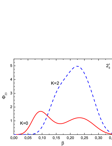
Figure 6: Distribution over $\beta$ of the squares of the components of the $2^{+}_{3}$ state with $K$=0 (solid line) and $K$=2 (dashed line) calculated according (18).

The experimental value of the excitation energy of the $3^{+}_{1}$ state and the value of B(E2; $3^{+}_{1}\rightarrow 2^{+}_{1}$) are reproduced by the calculations quite well. However, the experimental value of B(M1; $3^{+}_{1}\rightarrow 2^{+}_{1}$)=0.3 $\mu_{N}^{2}$ is too large to be reproduced in the framework of the collective model. For instance, the value of B(M1; $3^{+}_{\gamma}\rightarrow 2^{+}_{\gamma}$) for transition between the states of the $\gamma$-band in ¹⁶⁸Er is equal to 0.003 $\mu_{N}^{2}$ only, i.e. two orders of magnitude less than the value for ⁹⁶Zr. It could mean that the $3^{+}_{1}$ state of ⁹⁶Zr has a large component of the shell model neutron configuration $(s^{1}_{1/2}d^{-1}_{5/2})_{3}$ or even its structure is almost exhausted by this configuration Witt . We mention, however, that the experimental value of B(E2; $3^{+}_{1}\rightarrow 2^{+}_{1}$) can be reproduced only if both states have a collective admixture, since for the explanation of the experimental B(E2; $3^{+}_{1}\rightarrow 2^{+}_{1}$) value the shell model neutron configurations $(s^{1}_{1/2}d^{-1}_{5/2})_{2,3}$ requires a neutron E2 effective charge equal to one. The calculated wave function of the $3^{+}_{1}$ state is almost completely localized in the deformed minimum: $W_{3_{1}}$=0.96.

The strong E2 transition between the $0^{+}_{3}$ and the deformed $2^{+}_{2}$ states is reproduced by our calculations because a significant part of the wave function of the $0^{+}_{3}$ state is localized in the deformed minimum of the potential (see Fig.3).

It is indicated in Witt that the $4^{+}$ states at 2750 keV and 2781 keV presented in nndc1 have been observed in one experiment each only and were never been confirmed. For this reason we disregard these states and compare the calculated characteristics of the $4^{+}_{1}$ state with the experimental data for the $4^{+}$ state observed at 2857 keV.

Our calculations reproduce the value of the very collective E2 transition $4^{+}_{1}\rightarrow 2^{+}_{2}$ which shows that the significant part of the wave function of the $4^{+}_{1}$ state is localized in the deformed minimum. This fact is confirmed by the distribution of the wave function of the $4^{+}_{1}$ state shown in Fig. 7. It is seen also that the wave function of the $4^{+}_{1}$ state is exhausted by the $K$=0 component. The calculated ratio B(E2; $4^{+}_{1}\rightarrow 2^{+}_{2}$)/B(E2; $2^{+}_{2}\rightarrow 0^{+}_{2}$) = 1.65 is close to the Alaga value 1.43 for axially deformed nuclei. A distribution of the $K$=0, 2 and 4 components of the wave function of the $4^{+}_{1}$ state indicates that the large part of the total wave function is indeed located in the deformed minimum. At the same time the calculated B(E2; $4^{+}_{1}\rightarrow 2^{+}_{1}$) value agrees within the limit of the experimental error with the observed value. The calculated ratio $\left(E(4^{+}_{1})-E(0^{+}_{2})\right)$/$\left(E(2^{+}_{2})-E(0^{+}_{2})\right)$ is equal to 2.14 which is close to the spherical limit. The experimental value of this ratio 1.98 practically coincides with the value for the spherical harmonic oscillator.

This astonishing apparent correspondence of the $4^{+}_{1}$ state’s properties to contradicting limits of the collective model can be understood from the following consideration. The dominant parts of the wave functions of the $2^{+}_{2}$ and $4^{+}_{1}$ states are located in the deformed minimum. However, smaller parts of the wave functions of these states are spread over the spherical minimum. This fact allows us to consider the $2^{+}_{2}$ and $4^{+}_{1}$ states as a mixture of the two dominant, lowest-lying spherical and deformed components, each. As a result of this mixing, the $4^{+}_{1}$ state with dominantly deformed character is shifted down in energy because it is the lowest $4^{+}$ state. At the same time, the predominantly deformed $2^{+}_{2}$ state is shifted up in energy since it is the second excited $2^{+}$ state. This lowering of the excitation energy of the 4+ state and this increase of the $2^{+}$ state’s energy in the deformed well leads to the observed significant reduction of the $R_{4/2}$ ratio from the value of $10/3$ expected for axially-deformed nuclei towards a smaller value closer to 2.

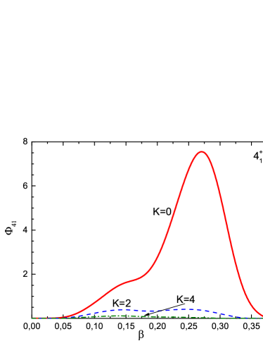
Figure 7: Distribution over $\beta$ of the squares of the components of the $4^{+}_{1}$ state with $K$=0 (solid), 2 (dashed) and 4 (dot-dashed) calculated according (18).

Let us analyze the result obtained for $\rho^{2}(0^{+}_{2}\rightarrow 0^{+}_{1})$ which is by factor 3 smaller than the experimental value. The definition of the $\rho^{2}(0^{+}_{2}\rightarrow 0^{+}_{1})$ value is given in (22). In order to get an expression for $\langle 0^{+}_{2}|\beta^{2}|0_{1}\rangle$ in terms of the quantities whose values are known from other experiments let us calculate the double commutator $[[H,\beta^{2}],\beta^{2}]$ using the Hamiltonian (5). The result is

$$\left[\left[H,\beta^{2}\right],\beta^{2}\right]=\frac{4\hbar^{2}}{B_{0}}\beta^{2}.$$ (24)

Taking the average of (24) over the ground state $0^{+}_{1}$ and assuming that the ground state is mainly related by $E0$ transition to the $0^{+}_{2}$ state we obtain

$$|\langle 0^{+}_{2}|\beta^{2}|0^{+}_{1}\rangle|^{2}\leq\frac{2\hbar^{2}}{B_{0}}\langle 0^{+}_{1}|\beta^{2}|0^{+}_{1}\rangle\frac{1}{E(0^{+}_{2})},$$ (25)

where $E(0^{+}_{2})$ is the excitation energy of the second $0^{+}$ state. The sign of inequality in (25) appears because we neglect a contribution into the value of $\langle 0^{+}_{1}|\beta^{2}H\beta^{2}|0^{+}_{1}\rangle$ of the other $0^{+}$ states higher in energy than $0^{+}_{2}$ . The quantity $\langle 0^{+}_{1}|\beta^{2}|0^{+}_{1}\rangle$ can be expressed with a good accuracy through the $B(E2;2^{+}_{1}\rightarrow 0^{+}_{1})$ value using the collective model definition of the $E2$ transition operator:

$$\langle 0^{+}_{1}|\beta^{2}|0^{+}_{1}\rangle=\displaystyle{\frac{5B(E2;2^{+}_{1}\rightarrow 0^{+}_{1})}{\left(\frac{3}{4\pi}ZeR^{2}\right)^{2}}}.$$ (26)

Substituting (25) and (26) into (22) we obtain

$$\rho^{2}(0^{+}_{2}\rightarrow 0^{+}_{1})\leq\frac{\hbar^{2}}{B_{0}}\frac{1}{E(0^{+}_{2})}\displaystyle{\frac{10B(E2;2^{+}_{1}\rightarrow 0^{+}_{1})}{e^{2}R^{4}}}.$$ (27)

In our calculations the value of $\dfrac{\hbar^{2}}{B_{0}}$ was fixed as 5 keV in order to reproduce the experimental value of $E(0^{+}_{2})$. Substituting this value and the calculated values of $E(0^{+}_{2})$ and $B(E2;2^{+}_{1}\rightarrow 0^{+}_{1})$ into (27) we obtain that

$$\rho^{2}(0^{+}_{2}\rightarrow 0^{+}_{1})\leq 0.005$$ (28)

in correspondence with the result given in Table 1.

This result means that we can not exclude that the pairing vibrational or some other modes play an important role in the description of the E0 transitions.

a)           b)

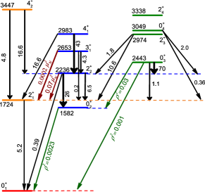
Figure 8: Experimental (a), nndc1 ; Witt ) and calculated (b) low-energy level scheme of positive-parity states of ⁹⁶Zr. Excitation energies are given in keV, B(E2) transitions are given in W.u.

All experimental data on low-lying excited states of ⁹⁶Zr are presented in Fig. 8a and the corresponding calculation results are shown in Fig. 8b. In both figures, states having very large spherical or deformed components are highlighted in two separate columns on the left. In Fig. 8b the division is based on the results of wave functions weights $W_{In}$ calculation which are shown in Table III. In contrast to the results Witt presented in Fig. 8a we placed the $4^{+}_{2}$ state among the spherical and $3^{+}_{1}$ state among the deformed ones based on the results shown in Table 3.

Table 3: The calculated weights $W_{In}$ in the spherical minimum of the considered states of ⁹⁶Zr.

State	$W_{In}$	State	$W_{In}$	State	$W_{In}$
$0^{+}_{1}$	0.985	$0^{+}_{2}$	0.136	$0^{+}_{3}$	0.292
$2^{+}_{1}$	0.772	$2^{+}_{2}$	0.182	$2^{+}_{3}$	0.289
$4^{+}_{2}$	0.636	$4^{+}_{1}$	0.139	$0^{+}_{4}$	0.202
		$3^{+}_{1}$	0.042	$2^{+}_{4}$	0.464

IV Conclusion

We have studied a possibility to describe the properties of the low-lying collective quadrupole states of ⁹⁶Zr basing on the Bohr collective Hamiltonian. Both $\beta$ and $\gamma$ shape collective variables are included into consideration. The $\beta$-dependence of the potential energy is fixed to describe the experimental data in a best possible way. However, a $\gamma$-dependence of the potential is introduced in a simple way favoring axial symmetry at large $\beta$. The resulting potential has two minima, spherical and deformed, separated by a barrier. The inertia tensor is taken in a diagonal form with the same values for both $\beta$- and $\gamma$-vibrational modes. However, the rotational inertia coefficient is taken to be 4 times smaller than the vibrational one in order to reproduce the excitation energy of the $2^{+}_{2}$ state. Rather good agreement with the experimental data is obtained for the excitation energies and the E2 transition probabilities. The calculated B(M1; $2^{+}_{2}\rightarrow 2^{+}_{1}$) value is two times smaller than the experimental value. Consideration of the $3^{+}_{1}\rightarrow 2^{+}_{1}$ M1 transition probabilities indicates the importance of knowledge of the microscopic structure of that part of the collective state wave function that is localized in the spherical minimum. At the same time our calculations show that the wave function of the $3^{+}_{1}$ state is localized mainly in the deformed minimum. Thus, our calculations indicate the problem in the description of the properties of the $3^{+}_{1}$ state of ⁹⁶Zr in the framework of the Geometrical Collective Model. The calculated value of $\rho^{2}(0^{+}_{2}\rightarrow 0^{+}_{1})$ is around three times smaller than the measured value. This indicates an influence of the other degrees of freedom that is not included in the present consideration.

V Acknowledgments

The authors express their gratitude to the RFBR (grant № 20–02-00176) and Heisenberg–Landau Program for support. One of the authors, N.P., thanks A. Leviatan, T. Otsuka, V. Werner, and T. Beck for discussion and gratefully acknowledges support by the DFG under grant N SFB1245 and by the BMBF under grant Nos. 05P19RDFN1 and 05P18RDEN9.

References

- (1) K. Heyde, J. L. Wood, Rev. Mod. Phys. 83, 1467 (2011).
- (2) K. Heyde, P. Van Isacker, M. Waroquier, J. L. Wood, and R. A. Meyer, Phys. Rep. 102, 291 (1983).
- (3) J. L. Wood, K. Heyde, W. Nazarewich, M. Huyse, and P. V. Duppen, Phys. Rep. 215, 101 (1992).
- (4) A. Poves, J.Phys. G: Nucl. Part. Phys. 43, 024010 (2016).
- (5) J. E. García-Ramos and K. Heyde, Phys. Rev. C 100, 044315 (2019).
- (6) T. Togashi, Y. Tsunoda, T. Otsuka, and N. Shimizu, Phys. Rev. Lett. 117, 172502 (2016).
- (7) K. Sieja, F. Nowacki, K. Langanke, and G. Martínez-Pinedo, Phys. Rev. C 79, 064310 (2009); Erratum, Phys. Rev. C 80, 019905(E) (2009).
- (8) J. E. García-Ramos, K. Heyde, R. Fossion, V. Hellemans, and S. De Baerdemacker, Eur. Phys. J. A 26, 221 (2005).
- (9) M. Böyükata, P. Van Isacker, and I. Uluer, J. Phys. G 37, 105102 (2010).
- (10) Y.-X. Liu, Y. Sun, X.-H. Zhou, Y.-H. Zhang, S.-Y. Yu, Y.-C. Yang, and H. Jin, Nucl. Phys. A 858, 11 (2011).
- (11) A. Petrovici, K. W. Schmid, and A. Faessler, J. Phys. Conf. Ser. 312, 092051 (2011).
- (12) R. Rodríguez-Guzmán, P. Sarriguren, L. M. Robledo, and S. Perez-Martin, Phys. Lett. B 691, 202 (2010).
- (13) J. Skalski, P.-H. Heenen, and P. Bonche, Nucl. Phys. A 559, 221 (1993).
- (14) J. Xiang, Z. P. Li, Z. X. Li, J. M. Yao, and J. Meng, Nucl. Phys. A 873, 1 (2012).
- (15) H. Mei, J. Xiang, J. M. Yao, Z. P. Li, and J. Meng, Phys. Rev. C 85, 034321 (2012).
- (16) J. Skalski, S. Mizutori, and W. Nazarewicz, Nucl. Phys. 617, 282 (1997).
- (17) C. Özen and D.J. Dean, Phys. Rev. C 73, 014302 (2006).
- (18) H. T. Fortune, Phys. Rev. C 95, 054313 (2017).
- (19) M. Büscher, R. F. Casten, R. L. Gill, R. Schuhmann, J. A. Winger, H. Mach, M. Moszyński, and K. Sistemich, Phys. Rev. C 41, 1115 (1990).
- (20) N. Gavrielov, A. Leviatan and F. Iachello, Phys. Rev. C 99, 064324 (2019).
- (21) M. Bender, P.-H. Heenen, and P.-G. Reinhardt, Rev. Mod. Phys. 75, 121 (2003).
- (22) T. Niksic, D. Vretenar, and P. Ring, Prog. Part. Nucl. Phys. 66, 519 (2011).
- (23) P. Federman, S. Pittel, and R. Campos, Phys. Lett. B 82 2 (1979).
- (24) K. Heyde, E.D. Kirchuk, and P. Federman, Phys. Rev. C 38, 984 (1988).
- (25) A. Etchegoyen, P. Federman, and E.G. Vergini, Phys. Rev. C 39, 1130 (1989).
- (26) A. Holt, T. Engeland, M. Hjorth-Jensen, and E. Osnes, Phys. Rev. C 61, 064318 (2000).
- (27) T. Niksic, D. Vretenar, G. A. Lalazissis, and P. Ring, Phys. Rev. Lett. 99, 092502 (2007).
- (28) C. Kremer, S. Aslanidou, S. Bassauer, M. Hilcker, A. Krugmann, P. von Neumann-Cosel, T. Otsuka, N. Pietralla, V. Yu. Ponomarev, N. Shimizu, M. Singer, G. Steinhilber, T. Togashi, Y. Tsunoda, V. Werner, and M. Zweidinger, Phys. Rev. Lett. 117, 172503 (2016).
- (29) T. Niksic, Z.P. Li, D. Vretenar, L. Prochniak, J. Meng, and P. Ring, Phys. Rev. C 79, 034303 (2009).
- (30) A. Bohr, Dan. Mat.-Fys. Medd. 26, 1 (1952).
- (31) D. A. Sazonov, E. A. Kolganova, T. M. Shneidman, R. V. Jolos, N. Pietralla, and W. Witt, Phys. Rev. C 99, 031304(R) (2019).
- (32) R. V. Jolos and P. von Brentano, Phys. Rev. C 76, 024309 (2007).
- (33) R. V. Jolos and P. von Brentano, Phys. Rev. C 77, 064317 (2008).
- (34) D. J. Rowe, P.S. Turner, and J. Repka, J. Math. Phys. 45, 2761 (2004).
- (35) M. A. Caprio, D. J. Rowe, and T. A. Welsh, Comput. Phys. Commun. 180, 1150 (2009).
- (36) D. J. Rowe and J. L. Wood, Fundamentals of Nuclear Models: Foundational Models(World Scientific, 2010).
- (37) M. A. Caprio, Phys. Rev. C 83, 064309 (2011).
- (38) D. R. Bes, Nuclear Phys. 10, 373 (1959).
- (39) W. Witt, N. Pietralla, V. Werner, and T. Beck, Eur. Phys. J. A 55, 79 (2019).
- (40) https://www.nndc.bnl.gov/ensdf/.
- (41) S. Iwasaki, T. Marumori, F. Sakata, and K. Takada, Prog. Theor. Phys. 56 (1976) 1140.