Irrealism from fringe visibility in matter-wave double-slit interference with initial contractive states
Abstract
The elements of reality coined by Einstein, Podoslky, and Rosen promoted a series of fundamental discussions involving the notion of quantum correlations and physical realism. The superposition principle applied in the double-slit experiment with matter waves highlights the need for a critical review of the adoption of physical realism in the quantum realm. In this work, we employ a measure of physical irrealism and consider an initial contractive state in the double-slit setup for which position and momentum variables of a single particle are initially correlated. We investigate how the behavior of the irrealism can help us to obtain information about the interference pattern, wavelike, and particle-like properties in the double-slit setup with matter waves. We find that there is a time of propagation that minimizes the irrealism, and around this point the state at the detection screen is squeezed in position and momentum in comparison with the standard Gaussian superposition. Interestingly, we show that the maximum visibility and the number of interference fringes are related to the minimum of the irrealism. Moreover, we demonstrate a monotonic relation between the irrealism and visibility around the time of minimum. Then, we argue how to use these results to indirectly measure the irrealism for position variable from the fringe visibility.
pacs:
03.75.-b, 03.65.Vf, 03.75.BeKeywords: Irrealism, double-slit, fringe visibility
I Introduction
The Loophole-free violation of Bell’s inequalities leaves no doubt that the classical deterministic notion of an objective reality calls for a critical review bell64 ; hensen15 ; giustina15 ; shalm15 . One could say that this idea starts with the celebrated work EPR35 of Einstein, Podolsky, and Rosen (EPR), where they introduced a sufficient condition to describe an element of physical reality. EPR wondered whether it was possible to ascribe realistic properties to a quantum system in the absence of measurements, bringing up a formal definition to probe physical realism in the context of quantum theory. Employing also a necessary criterion for completeness of a physical theory, they argued that quantum mechanics was incomplete since it would allow simultaneous elements of reality for incompatible observables. EPR’s criterion is related to certainly predict the value of some physical property, without disturbing it, then assuming also the condition of causality in space-time dieguez18 .
Bohr’s approach to that was in terms of his complementarity principle bohr35 , which says that the elements of reality of incompatible observables cannot be established in the same experiment, but only through mutually excluding experimental arrangements. The notion of wave particle duality, which arises in the complementarity principle, highlights the counterintuitive character of quantum mechanics. According to that, the same physical system can exhibit either a particle-like or a wave-like behavior Feynman ; Bohr depending on the specific design of a certain experiment. The nontrivial result of that principle is well illustrated with the so-called Wheeler’s delayed choice gedanken experiment. On the other hand, we know today that with the addition of a quantum-controlled device of the delayed-choice experiment, it is possible to challenge the complementarity principle by allowing the same experimental apparatus to measure wave-to-particle transitions Ionicioiu11 ; Auccaise12 ; Peruzzo12 ; Kaiser12 .
Matter-waves quantum interference, another notable aspect of nature in which massive particles exhibit spatial delocalization, completely challenging our classical intuition about physical realism, is also a subject of intense research given its importance to the foundations of quantum theory. Experiments reveling wave-particle duality in the double-slit were performed by Möllenstedt and Jösson for electrons Jonsson , by Zeilinger et al. for neutrons Zeilinger1 , by Carnal and Mlynek for atoms Carnal , using diffraction gratings by Schöllkopf and Toennies for small molecules Toennies , by Zeilinger et al. for macromolecules Zeilinger2 , and electron double-slit diffraction has been experimentally observed in Bach . Moreover, the Einstein-Bohr debate about the wave-particle duality in the “floating” double-slit gedanken experiment, has recently been explored in liu2015 . Using molecules as slits, this provides an experimental proof and theoretical support showing that a Doppler marker eliminates the interference pattern, in corroboration with Bohr’s complementary principle liu2015 . Interestingly, this consideration goes against the logic initially advocated by EPR and emphasizes the role of correlations generated in the experimental configuration bilobran15 ; angelo15 ; dieguez18 as a fundamental mechanism to the emergence of physical realism.
Conceptually different from quantum correlations between two systems or two different Hilbert spaces of a single system (for example, spin and position degrees of freedom), position-momentum correlations are correlations that indicate a dependence between the position and the momentum of a single particle. In the case of a simple Gaussian or minimum-uncertainty wavepacket solution for the Schrödinger equation for a free particle, the position-momentum correlations at are zero but they appear for later times Bohm ; Saxon . On the other hand, more complex states such as squeezed states or a linear combination of Gaussian states can exhibit initial correlations, i.e., correlations that do not depend on the time evolution Robinett ; Riahi ; Dodonov ; Campos . It was shown that the existence of position-momentum correlations is related with the phases of the wave function Bohm . The position-momentum correlations can also be used to gain information about other relevant physical quantities. For example, qualitative changes were shown in the interference pattern as a function of the increase in the position-momentum correlations Carol . The Gouy phase matter waves are directly related to the position-momentum correlations, as studied in Ref.Paz1 . A relation was observed between the position-momentum correlations and the formation of above-threshold ionization (ATI) spectra in the electron-ion scattering in strong laser fields Kull . More recently, it was shown that the maximum of the position-momentum correlations is related with the minimum number of interference fringes in the double-slit experiment solano .
In this work, we use the facts that the measure of physical (ir)realism introduced by Bilobran and Angelo bilobran15 for discrete-spectrum observables is quantitative, operational, and was further extended for continuous variables in freire19 , thus allowing us to make formal connections of this quantity, and other measures such as wave-like and particle-like properties in the double-slit experiment with matter waves modeled by a contractive state Yuen , to verify how the evolution of the fundamental and entropic uncertainties affects these measures. This paper is structured as follows. In Sec. II, we introduce and briefly discuss the main properties of the measure of the degree of irrealism developed in bilobran15 . In Sec. III, we model the double-slit experiment with matter waves considering an initially contractive Gaussian wavepacket, which propagates during the time from the source to the double-slit and during the time from the double-slit to the screen. We calculate the wave functions for the passage through each slit using the Green’s function for the free particle to obtain the position-momentum correlations, the fundamental and entropic uncertainties, and the irrealism for this system that is a linear combination of the states that passed through each slit. We show that these quantities are minima at the same propagation time from the source to the double-slit. On the other hand, the position-momentum correlations and the fundamental uncertainties have a common point of maximum that does not coincide with the maximum irrealism. In Sec. IV, the relative intensity, visibility, and predictability are analyzed in terms of the minimum and maximum of the irrealism. For the viewpoint of comparison, we also analyze these quantities for the maximum of the position-momentum correlations. Here, it was proposed to indirectly measure the irrealism from the fringe visibility around the time of minimum. In Sec. V we present our concluding remarks.
II Irrealism and quantum theory
There is not a single formalism to discuss the concept of realism in quantum theory, and we should not be surprised about it if we remember that there is also not a unified interpretation of the consequences of the basic axioms of quantum theory. Indeed, the puzzle of defining realism in quantum theory invariably touches other foundational questions, such as the measurement problem and wave-particle duality. For example, in a traditional double-slit setup, does the quantum system pass through both slits simultaneously, acting somehow like a definite wave, or we should interpret it as a state of fundamental local indefiniteness in that region of space-time? What has to be considered as a physical premiss to probe physical realism in this context?
When questioning whether it was possible to attribute realism to entangled quantum systems, EPR was based both on the completeness of a physical theory and also on a sufficient condition that would define realistic aspects. According to EPR, the necessary condition assumed for a physical theory to be considered complete is that every element of physical reality must have a correspondence in the theory EPR35 . To conduct their analysis in what concerns the elements of physical reality, they define the following sufficient condition: “If, without disturbing the system in any way, we can predict with certainty the value of a physical quantity, then there is an element of physical reality corresponding to this quantity”. When applied to spins, this condition can be stated as follows. Suppose the singlet state, . After the formation of this entangled pair, it is clear that under a measurement on one of the systems, the spin in the same direction of the other can always be anticipated with certainty since this correlation is preserved in all bases. Then, according to EPR there must be an element of physical reality corresponding to this physical quantity. Note that this conclusion is independent of the spatial distance between the systems, thus it is possible to assume a strong version of relativistic causality vaidman96 , that is, no space-like event could perturb the local results. A deep consequence of that argument, together with the fact that we can measure the spin along any direction and the correlation is the same, is that the fact of an exact prediction on a distant system invites us to interpret this as the mere manifestation of a pre-existing value of this physical property, since both systems did not interact while the measurement was carried out. This implies that incompatible observables also have their elements of reality defined independently. Since quantum theory generally does not give us this value for observables that do not commute, EPR concluded that although correct, it gives an incomplete description of reality, being necessary as discussed by EPR, the so-called hidden variables that would complete the theory. As we know today, no set of hidden local variables is capable of reproducing all the results of experiments with entangled states. Furthermore, as EPR attributes realism only to properties that can be predicted with certainty, such a criterion does not include the class of mixed states that have their probabilities linked to a purely subjective ignorance, as in the case of epistemic states.
To discuss the definition of physical realism in the double-slit experiment with matter waves, we review in this section, a quantifier introduced by Bilobran and Angelo bilobran15 , which put forward an operational scheme to assess elements of reality of discrete-spectrum observables in quantum mechanics and generalizes EPR’s definition. The main idea of this measure is constructed under the premise that a measurement establishes the reality of an observable even if we do not have access to the result of this measurement, thus indicating realism also for an epistemic state, which is a state that has only subjective ignorance.
This can be formally stated with the following procedure. Bilobran and Angelo bilobran15 consider a preparation that acts in submitted to a protocol of unrevealed measurements (also known as non-selective measurements) of a generic observable , with projectors , acting on . Since the outcome of the measurement is considered unrevealed in this protocol, the resulting state is the average over all possible results,
| (1) |
where and . Bilobran and Angelo propose to take as a state of reality for and as a formal criterion of reality. Note that this premise of realism also agrees with the EPR criterion, since eigenstate preparations are elements of reality for some observable, but this also attempts to generalize EPR in a sense that it also quantifies the degree of realism for mixed states. With that, by employing the relative entropy , they compute the degree of irrealism of the observable given the preparation as
| (2) |
where is the von Neumann entropy. Note that, this quantifier is non-negative and vanishes if and only if , thus allowing us to interpret it as an “entropic distance” between the state and the state that obeys realism for this observable . As discussed in bilobran15 ; freire19 , although one could use some other norm, the use of the “entropic metric” allows one to relate this measure with other quantities of quantum information theory. For example, the above formula can be decomposed as
| (3) |
where stands for the nonminimized version of the one-way quantum discord (see Refs. bilobran15 ; dieguez18 for further details). So, the irrealism of is the sum of local coherence (that is, the coherence of given the reduced state ) with quantum correlations associated with measurements of . Then, for single-partite states ( which acts in ) or uncorrelated bipartite states, the irrealism reduces to the amount of quantum coherence relative to the -Basis baumgratz14 . This observation highlights the contextual character of irrealism, since it is an observable and also a state-dependent quantity.
This approach gives a prominent role to the notion of information. Indeed, by employing a model of measurement called monitoring dieguez18 ; dieguez2018 , it was deduced that there is a formal connection between information and reality in quantum mechanics, developing a complementarity relation to these concepts dieguez18 . By now, this measure has proven relevant in scenarios involving coherence angelo15 , nonlocality gomes18 ; gomes19 ; fucci19 , weak reality dieguez18 , which also has an experimentally verification with photonic weak measurements mancino18 , realism-based entropic uncertainty relations rudnicki18 , random quantum walk orthey19 , Hardy’s paradox engelbert20 , and more recently, from the point of view of a generalized resource theory of information costa20 . Nevertheless, all of these works are exclusively applied to discrete spectrum observables. To fill this gap, Freire and Angelo presented a framework in freire19 , which calculates the degree of realism associated with continuous variables such as position and momentum by explicitly presenting a formalism through which one can quantify the degree of irrealism associated with a continuous variable for a given quantum state, by showing how to consistently discretize the position and momentum variables in terms of operational resolutions of the measurement apparatus. With that, they implemented an operational notion of projective measurement and a criterion of reality for these quantities. Interestingly, they introduced a quantifier for the degree of irrealism of a discretized continuous variable, which, when applied to pure states, exhibits an uncertainty relation to the conjugated pair position-momentum, as
| (4) |
meaning that quantum mechanics, equipped with Heisenberg’s uncertainty relation, prevents classical realism for conjugated quantities freire19 .
In this work, we propose to apply these ideas to formally analyze how position and momentum elements of reality behave in situations in which massive particles produce an interference pattern due to a coherent superposition in the double-slit setup, in order to interpret this state as assuming a purely physical uncertainty regarding its reality. So, in what follows we discuss how we model our double-slit setup and discuss how we quantify the degree of irrealism in such a context.
III Irrealism in the double-slit experiment
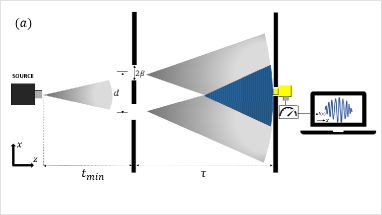
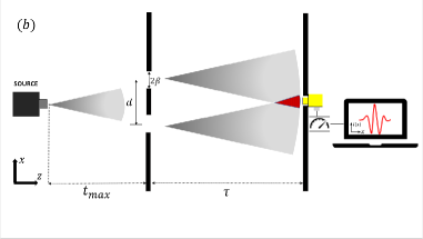
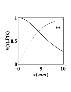
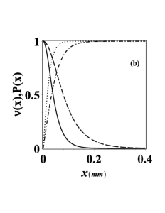
In this section, we model the double-slit experiment as follows. Before reaching the double-slit setup, we consider that a coherent Gaussian wave packet of initial width correlated in position and momentum propagates during a time before arriving at a double-slit that divides it into two Gaussian wavepackets. These initial correlations are measured by a parameter , such that, for , the state is spread in momentum but acquires a portion of correlations such that the Robertson-Schrödinger uncertainty relation attains the minimum value of . It has been shown that this state is not squeezed in terms of the conventional position and momentum operators but it exhibits squeezing for the generalized quadrature operators defined through the conventional operators by a rotation in the phase space IGP2020 . After the double-slit, the two wavepackets propagate during a time until they reach the detection screen, where they are recombined and the interference pattern is observed as a function of the transverse coordinate . Here, we consider a one-dimensional problem such that the momentum in the direction is very high and produces a very small wavelength and negligible quantum effects. Then, we treat this direction as classical, and the quantum effects are observed in the direction. As a consequence of the free propagation, which decouples the , , and dimensions for a given longitudinal location, we can write for the direction. The position and momentum of the particle will be correlated, and such correlations, as well as the fundamental and entropic uncertainties, will be changed by the evolution and the parameter . This model is presented in Fig.1 together with illustrations of the behave that will be found in the results. In Fig.1(a) the initial wavepacket propagates a time from the source to the double-slit, which produces at the detection screen the maximum region of overlap, interference fringes, and visibility. As we will see in the results, this propagation time corresponds to the minimum position-momentum correlations, fundamental and entropic uncertainties, and irrealism. In Fig.1(b), the initial wavepacket propagates a time from the source to the double-slit, which produces at the detection screen a small region of overlap with a small number of interference fringes and visibility. As we will see later on, this propagation time corresponds to the maximum position-momentum correlations and fundamental uncertainties, which are different from the time for the maximum irrealism.
The wavefunction at the time when the wave passes through the upper slit or the lower slit is given by Carol
| (5) | |||||
where the kernels and are the free propagators for the particle,
| (6) |
| (7) |
the function describes the double-slit transmission functions, which are taken to be Gaussian of width separated by a distance ,
| (8) |
and considering the initial wave function as
| (9) |
Here, we consider that is the transverse width of the initial wavepacket, is the mass of the particle, () is the time of flight from the first slit (double-slit) to the double-slit (screen). The parameter ensures that the initial state is correlated in position and momentum. In fact, we obtain for the initial state the following results for the uncertainties in position and in momentum, and , and for the position-momentum correlations . For , we have the simple uncorrelated Gaussian wavepacket and for , we have a contractive state Yuen . As we can observe the Robertson-Schrödinger uncertainty relation attains the minimum value independent of .
To obtain analytic expressions for the fundamental uncertainties, position-momentum correlations, relative intensity, visibility, and predictability in the screen of detection, we use a Gaussian transmission function instead of a top-hat transmission function because a Gaussian transmission function represents a good approximation to the experimental feasibility and also because it is mathematically simpler to treat than a top-hat transmission function. The corresponding wavefunction for the propagation through the upper slit was previously obtained in Ref. oziel , and it is given by
| (10) | |||||
where the wave-function parameters and their physical meanings are discussed as follows. The classical optics analogous of the radius of curvature of the wavefronts for the propagation through one slit is
| (11) |
with , and is one intrinsic time scale (the half of the Ehrenfest time) which essentially corresponds to the time during which a distance of the order of the wavepacket extension is traversed with a speed corresponding to the dispersion in velocity Roman . It is viewed as a characteristic time for the “aging” of the initial state Carol ; solano , since it is a time from which the evolved state acquires properties completely different from the initial state. The wavepacket width for the propagation through one slit is
| (12) |
is a time dependent wavenumber
| (13) |
is the separation between the wavepackets produced in the double-slit
| (14) |
is the wavepacket width for the free propagation
| (15) |
is the classical optics analogous of the radius of curvature of the wavefronts for the free propagation
| (16) |
and is the Gouy phase for the propagation through one slit
| (17) |
Note that and ,
| (18) |
are time dependent phases and they are relevant only if the slits have different widths. Also, to obtain the expressions for the wave function passing through the lower slit, we just have to substitute the parameter by in the expressions corresponding to the wave passing through the upper slit. Different from the results obtained in Ref. solano , all the parameters above are changed by the correlation parameter .
Now we are in a position to discuss how we evaluate the irrealism for the wavefunction at the detection screen. First, we note that for single partite pure states, it follows that , and the von Neumann entropy of this state when the unread measurement map is applied reduces to , where is the Shannon entropy associated with probability distributions for the variables (see freire19 for more details). To construct the Shannon distribution of the discretized continuous variable , we follow the main idea of Refs. birula84 ; partovi83 to write the discretized probability distribution of a position measurement in terms of experimental resolutions for position measurements of . However, since the expressions used in birula84 ; partovi83 are known to be ill-behaved in the limit of large coarse-graining for some states rudnicki11 , here we take a slightly different strategy discussed in rudnicki11 , which corrects this problem by introducing a symmetrical limit to compute the discretization procedure as
| (19) |
where is the probability density in position, and
| (20) |
is the normalized wavefunction in the screen of detection.
Note that we made a discretization of the probability distribution in terms of the experimental resolution , which is assumed to be a constant. Moreover, with the introduction of the above symmetrical limit, which realizes that one shall investigate the limit of large experimental accuracies rudnicki11 , we guarantee two important aspects of the irrealism measure. In their seminal paper, Bilobran and Angelo conceived it as an operational measure by adopting a measurement-based premise, thus linking the irrealism with the capabilities of the measurement apparatus. Furthermore, it was also shown in dieguez18 that the irrealism is intimately related to the concept of information in quantum theory. So, it is expected that the irrealism goes to zero in the limit of very inaccurate experimental resolutions (see freire19 for more details), in the same way that very imprecise performed measurements tell us nothing about the information of quantum states. With that, we can calculate the Shannon entropy as
| (21) |
and now it is straightforward to calculate the corresponding degree of irrealism for the position of the state (20), explicitly by
| (22) |
For the momentum in terms of the wavevector , we follow the same strategy to write
| (23) |
with
| (24) |
where is obtained with the corresponding Fourier transform of , and is the discretized probability for momentum measurements with resolution .
III.1 Fundamental uncertainties relations
In what follows, we calculate the fundamental uncertainties in position and momentum, the position-momentum correlations, and the generalized Robertson-Schrödinger uncertainty relation in the detection screen. The fundamental uncertainties are important to establish the limit in which experimental resolutions would not be able to access quantum information. We will show that the fundamental uncertainties and the position-momentum correlations have a minimum and a maximum common point as a function of the propagation time for a negative value of the correlation parameter (contractive state). For positive or null values of these quantities have only a maximum, no minimum. On the other hand, the Robertson-Schrödinger uncertainty relation has the same common point of minimum for a contractive state, but it does not have a maximum independent of the value and signal of .
For the normalized wavefunction Eq.(20), we calculate the fundamental uncertainties in position and momentum, and the position-momentum correlations, and we obtain, respectively,
| (25) |
| (26) | |||||
and
| (27) | |||||
The determinant of the covariance matrix is the generalized Robertson-Schrödinger uncertainty relation, and it is given by
| (28) |
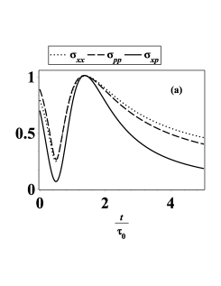
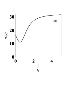
In the following, we plot the curves for the uncertainties in position, in momentum, the position-momentum correlations, and the Robertson-Schrödinger uncertainty as a function of the time for neutrons. The reason to consider neutrons relies on their experimental feasibility, which is most close to our model for interference with completely coherent matter waves, although we still have a loss of coherence as discussed in Ref.Sanz . We adopt the following parameters: mass , initial width of the packet (which corresponds to the effective width of ), slit width , the separation between the slits , and de Broglie wavelength . These same parameters were used previously in double-slit experiments with neutrons by Zeilinger et al. Zeilinger1 . In Fig.2(a) we show the plot of the uncertainties in position, momentum, and the position-momentum correlations. In Fig.2(b) we show the Robertson-Schrödinger uncertainty as a function of for , and for an initial contractive state . We use arbitrary normalization constants to have the three curves at the same plot in Fig.2(a). The dotted line corresponds to the uncertainty in position, the dashed line corresponds to the uncertainty in momentum, and the solid line corresponds to the position-momentum correlations. As we can observe, these quantities have common points of minimum and maximum that we calculate and obtain, respectively, as and . On the other hand, the Robertson-Schrödinger uncertainty has the same point of minimum but it does not have a point of maximum, which is a consequence of how the position-momentum correlations evolve with time.
A very interesting result is that despite the fact that the difference for the times of maximum and minimum is smaller than unity in terms of , these values of time produce interference and fringe visibility that are completely distinct, as we will see later on.
III.2 Irrealism and fundamental uncertainties
Following the formalism put forward in bilobran15 ; dieguez18 ; freire19 , we present our results concerning the degree of irrealism in position and momentum variables for different experimental resolutions applied to our interferometer model. In particular, the fundamental uncertainties play an important role in the experimental resolution of the apparatus employed to probe the irrealism for continuous variables observables such as position and momentum. As long as the apparatus resolution is such that , we have positive values for the irrealism in position and momentum variables. Despite the dependence on the experimental resolution, we will show that we have the same time evolution for each different experimental resolution. Another important limit for the irrealism measure, discussed in greater detail in freire19 , emerges when , since we have for this low-resolution regime. On the other hand, note that it is perfectly legitimate to explore the continuous limit of the Shannon entropy by following, for example, the procedure given in Coles , , to compute the limit, which produces for Gaussian states, and for general states. However, here we focus on the operational meaning of irrealism coined in bilobran15 , and we present our results in terms of experimentally feasible states , with for the role of the apparatus in our double-slit interferometer setup, instead of thinking in the idealized eigenstates . Also, one can follow the formalism discussed in freire19 to propose a change of variables that produces an experimental independent expression for the irrealism. In the following, we propose a useful way of rescaling the irrealism measure in comparison with the minimum value associated with the experimental resolutions that limit the extraction of irrealism, this is, in terms of the fundamental uncertainty of the system. We consider , and we rewrite the irrealism in Eq. (22) as
| (29) | |||||
where is the integration interval for which the probability is normalized to and the resolution is related with and by . We can obtain a similar expression for the momentum irrealism.
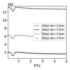
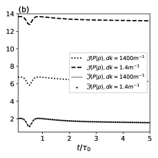
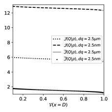
Different from the fundamental uncertainties, the irrealism in position and momentum variables needs to be calculated numerically since we do not have closed expressions for this particular state. Therefore, we perform numerical calculations and exhibit them in Fig.3. In Fig.3(a) we show the plot of the irrealism in position and in Fig.3(b) the irrealism in momentum as a function of for and . We consider and as the experimental resolution of reference. Then, we use two experimental resolutions and for the irrealism in position, and and for the irrealism in momentum, which show that the rescaled irrealism of Eq.(29) is resolution-independent. In the same plot we exhibit the irrealism for these two experimental resolutions, which show that we have more irrealism with the increasing use of higher-resolution apparatuses. From these results, we see that the relevant physical content is clearly related to the temporal evolution of this quantity. Furthermore, with the rescaling irrealism proposed here, experimentalists could directly use their data, without having to make changes of variables and without bothering with the limit of a higher-resolutions apparatus, since the most important aspect of this model is to employ an apparatus that has more resolution than the fundamental one, which is attached with the uncertainty principle. The irrealism for each resolution is minimum at the same time for which the fundamental uncertainties and position-momentum correlations are minima, i.e., . However, the time for the maximum irrealism is which does not coincide with the time of maxima position-momentum correlations.
Note that, by employing such a normalization procedure, we are not claiming that this version is more fundamental than the previous one with the explicit dependence on its experimental resolution. The normalization introduced here could be important for comparing more directly the results obtained previously with different experimental resolutions for the double-slit interferometer setups with matter waves. Before that, it is interesting to discuss the existence of a point of minimum. Following Bohm in Ref. Bohm , the position-momentum correlations are correlations that develop with the quantum dynamics producing a minimum Robertson-Schrödinger uncertainty relation for a Gaussian wavepacket. Also, in Bohm’s words, large correlations mean that a high momentum tends to become correlated with the covering of a large distance. In this case, minima correlations imply minimum position and momentum uncertainties that corroborate our results. We can also understand the existence of minima fundamental and entropic uncertainties from the viewpoint of squeezing. It has been shown that the initial contractive state produces a squeezed superposition in comparison with the standard Gaussian superposition at the detection screen of a double-slit experiment IGP2020 . In Fig.4 we show the uncertainties in position and in momentum for the superposition at the detection screen when , normalized by the respective uncertainties for the standard Gaussian superposition, i.e., when . We can observe squeezing in position and momentum around the point of minimum .

Therefore, the minimum observed here for the fundamental uncertainties and irrealism is a consequence of squeezing present in the superposition when the initial state is a contractive state. This result presents a similar behavior to the result obtained in Fig.14 of Ref.Coles for the EPR state Weedbrook , which shows a decreasing in the entropic uncertainty as a function of the squeezing strength. Squeezing also means a large region of overlap between the two packets for the time for which the uncertainties and irrealism are minima. Therefore, when the superposition created in the double-slit is squeezed/localized in the detection screen to produce minimal uncertainties and a large region of overlap, which means that one can not distinguish the packets in the superposition, the irrealism tends to be minimum. These results are also reflected in the interference pattern, as we can observe in the next section.
IV Irrealism and fringe visibility
It has been shown that wave-particle duality relations are actually entropic uncertainty in disguise. Also, an expression has been found that involves minimum and maximum entropies and unifies the wave-particle duality principle with the entropic uncertainty principle; see Eq.(344) of Ref.Coles . Here, we calculate the relative intensity, visibility, and predictability to analyze the interference pattern as well as the wave and particle properties from the knowledge of the minimum and maximum irrealism. The minimum entropy, i.e., minimum irrealism, is characterized by a maximum number of interference fringes and maximum visibility. The maximum irrealism is characterized by a small number of interference fringes and small visibility. We also study the interference pattern, the visibility, and predictability around the time for which the fundamental uncertainties and position-momentum correlations are maximal.
The intensity on the screen is given by
| (30) |
where
| (31) |
The first term in Eq.(30) is the single-slit envelope, and the second term is the interference solano . From Eq.(30), we obtain the expression for the relative intensity,
| (32) |
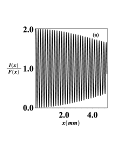
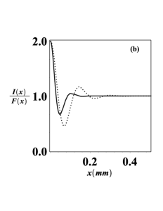
In Fig.5, we show half of the symmetrical plot for the relative intensity as functions of for an initial contractive state. In Fig. 5(a) we consider the time for which the irrealism is minimum, i.e., . In Fig. 5(b) we consider the time for which the irrealism is maximum, i.e., (dotted line) and the time for which the fundamental uncertainties and position-momentum correlations are maximal, i.e., (solid line). We fixed the propagation time from the double-slit to the screen in . We observe a large number of interference fringes associated with the minimum irrealism and a small number of interference fringes associated with the maximum irrealism. A smaller number of interference fringes are observed for the time of maxima fundamental uncertainties and position-momentum correlations.
The knowledge of both “particle” and “wave” in an interferometric experiment is given by the Greenberger and Yasin expression , where stands for particle property and for wave property. The parameter () is used to vary from full particle to full wave knowledge preserving the general case in which one can have considerable knowledge of both. The equality is ensured for pure quantum-mechanical states and the inequality for mixed states Greenberger . We calculate the predictability and visibility for our experimental setup and obtain
| (33) |
and
| (34) |
where is the intensity for and is the intensity for solano . Similar results were obtained previously in Ref. Bramon .
In Fig.6(a) we show half of the symmetrical plot of the visibility (solid line) and predictability (dotted line) as functions of for the time for which the fundamental and entropic uncertainties, as well as the irrealism, are minimal. In Fig. 6(b) we show half of the symmetrical plot of the visibility (solid line) and predictability (dotted line) as functions of for the time for which the fundamental uncertainties and the position-momentum correlations are maximal, and the plot of the visibility (dashed line) and predictability (dash-dotted line) for the time for which the irrealism is maximum. As before, we fixed the propagation time from the double-slit to the screen in .
These results show clearly the relationship between the minimum of the entropic uncertainty and irrealism with the maximum number of interference fringes and visibility (wave character) in the double-slit experiment. The wave property is predominant in a larger region of the axis when the irrealism is minimum and the particle property is dominant around the maximum irrealism, as we can observe by comparing the curves of visibility and predictability for the times of minimum and maximum irrealism. These results are according to the connection obtained in Ref.Coles , which associates the wave-particle duality with minimum and maximum entropy.
The results above suggested that for the point of minimum the irrealism can be obtained from the visibility. We find that around this point the irrealism can be approximated by the equation
| (35) |
where and are constants to be found in the adjustment, and is the fringe visibility measured in the position equal to the wave-packet separation while the source is placed in the position . Then, each value of which gives a specific value for and produces a specific value for the visibility and irrealism. In Fig.7 we show the plot for the irrealism in position as a function of . The full circle curve is the numerical calculation, and solid curve is the adjustment Eq. (35). In adjusting we find and . We can observe from Eq. (35) and Fig.7 that the minimum irrealism is related with the maximum visibility. Furthermore, as we can see in the parametric plot, these results show a monotonic relation between irrealism and visibility in the right plot of Fig. 7. As expected, we observe the same behavior for the irrealism and the rescaled one.
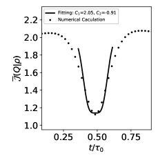
Therefore, around the point of minimum, where the visibility is large, one can measure the fringe visibility as a function of and use Eq. (35) to obtain the corresponding measurement of irrealism.
V Conclusions
The purely epistemic uncertainty present in classical statistical physics does not reflect the irrealism of the physical properties of these systems. In addition to our statistical ignorance, these properties are already predetermined before any measurement in such a classical regime; in this case, the uncertainty reflects only subjective ignorance. On the other hand, quantum superposition, which lies at the heart of the quantum theory, points out that reality seems to be in suspension in such cases, that is, physical properties do not have well-defined values that support physical realism. This gives rise to many of the contra-intuitive interpretations of quantum theory since even molecules exhibit this condition. This ontological uncertainty implies that the classical notion of realism is forbidden in general for two noncommuting observables such as position and momentum, as demonstrated in freire19 .
In this work, employing the quantifier introduced in freire19 , and proposing a rescaling in terms of the fundamental uncertainties, we have taken a step further on this issue by exploring the consequences of an initial contractive state to the degree of position and momentum irrealism in double-slit configuration for massive particles interference. We analyzed the connection of physical irrealism and fundamental uncertainties, with the intensity, visibility, and predictability of the wavepackets interference. We saw that the propagation time that minimizes the fundamental uncertainties and the irrealism in position or momentum are the same. This minimum is related to the squeezing present in the superposition for an initial contractive state, since a non-contractive state has only a maximum value. By analyzing the behavior of the visibility and predictability for the minimum and maximum times, we saw that minimum irrealism coincides with the maximum number of interference fringes and visibility for this configuration, while predictability is dominant in the region of maximum irrealism. Moreover, this coincidence in the minimum indicates that it is possible to estimate irrealism if we look at visibility at this same point of the minimum. Indeed, we proposed here a way to indirect probe irrealism in the context of matter-wave double-slit interference by probing the fringe visibility.
Finally, the results of this work are important to the proposal of a successful interference experiment, indicating how to define values for parameters that can produce a maximum number of fringes with better visibility. This is also important from the perspective of the foundations of quantum theory, indicating that there is a minimum value for the irrealism of the studied system that produces the maximum interference in the context of matter waves, which allows us to reinterpret the double-slit experiment with the initial contractive state by employing a notion of a state with fundamental physical indefiniteness, instead of thinking of a particle traveling as a definite wave. This highlights the quantum nature of this mechanism of interference and the lack of reality of that systems. We hope that the results developed here help to encourage experimentalists to implement an indirect measurement of irrealism to matter waves.
Acknowledgements.
The authors would like to thank the anonymous referees for their many insightful comments and suggestions. The authors acknowledge CAPES and CNPq-Brazil for financial support. P.R.D. acknowledges Grant No. 88887.354951/2019-00 from CAPES. I. G. da Paz acknowledges Grant No. 307942/2019-8 from CNPq.References
- (1) J. S. Bell, Physics 1, 195 (1964).
- (2) B. Hensen et al., Nature (London) 526, 682 (2015).
- (3) M. Giustina, M. A. M. Versteegh, S. Wengerowsky, J. Handsteiner, A. Hochrainer, K. Phelan, F. Steinlechner, J. Kofler, J. Å. Larsson, C. Abellan et al., Phys. Rev. Lett. 115, 250401 (2015).
- (4) L. K. Shalm, E. Meyer-Scott, B. G. Christensen, P. Bierhorst, M. A. Wayne, M. J. Stevens, T. Gerrits, S. Glancy, D. R. Hamel, M. S. Allman et al., Phys. Rev. Lett. 115, 250402 (2015).
- (5) A. Einstein, B. Podolsky, and N. Rosen, Phys. Rev. 47, 777 (1935).
- (6) P. R. Dieguez and R.M. Angelo, Phys. Rev. A 97, 022107 (2018).
- (7) N. Bohr, Phys. Rev. 48, 696 (1935).
- (8) R. Feynman, R. B. Leighton and M. L. Sands, The Feynman Lectures on Physics: Quantum Mechanics vol 3 (Addison-Wesley, Reading, MA, 1965), Vol. 3, Chap. 1.
- (9) N. Bohr, Nature 121, 580 (1928); W. K. Wootters and W. K. Zurek, Phys. Rev. D. 19, 473 (1979).
- (10) R. Ionicioiu and D. R. Terno, Phys. Rev. Lett. 107, 230406 (2011).
- (11) R. Auccaise, R. M. Serra, J. G. Filgueiras, R. S. Sarthour, I. S. Oliveira, and L. C. Céleri Phys. Rev. A 85, 032121 (2012).
- (12) A. Peruzzo, P. Shadbolt, N. Brunner, S. Popescu, and J. L. O’Brien, Science 338, 634 (2012).
- (13) F. Kaiser, T. Coudreau, P. Milman, D. B. Ostrowsky, and S. Tanzilli, Science 338, 637 (2012).
- (14) G. Möllentedt and C. Jönsson, Z. Phys. 155, 472 (1959).
- (15) A. Zeilinger, R. Gähler, C. G. Shull, W. Treimer, and W. Mampe, Rev. Mod. Phys. 60, 1067 (1988).
- (16) O. Carnal and J. Mlynek, Phys. Rev. Lett. 66, 2689 (1991).
- (17) W. Schöllkopf and J. P. Toennies, Science 266, 1345 (1994).
- (18) M. Arndt et al., Nature, 401 680, (1999); O. Nairz, M. Arndt, and A. Zeilinger, J. Mod. Opt., 47, 2811 (2000); Am. J. Phys. 71, 319 (2003).
- (19) R. Bach, D. Pope, S. Liou, and H. Batelaan, New J. Phys. 15 033018, (2013); S. Frabboni, G. C. Gazzadi, and G. Pozzi, Appl. Phys. Lett. 93, 073108 (2008).
- (20) X. J. Liu, Q. Miao, F. Gel’mukhanov, M. Patanen, O. Travnikova, C. Nicolas, H. Ågren, K. Ueda, and C. Miron, Nat. Photonics 9, 120 (2015).
- (21) A. L. O. Bilobran and R. M. Angelo, Europhys. Lett. 112, 40005 (2015).
- (22) R. M. Angelo and A. D. Ribeiro, Found. Phys. 45, 1407 (2015).
- (23) D. Bohm Quantum Theory (Prentice-Hall, Englewood Cliffs) pp. 200-205 (1963).
- (24) D. S. Saxon Elementary Quantum Mechanics (McGraw-Hill, New York, 1968), pp. 62-66.
- (25) R. W. Robinett, M. A. Docheski, and L. C. Bassett, Found. Phys. Lett. 18, 455 (2005).
- (26) N. Riahi, Eur. J. Phys. 34, 461 (2013).
- (27) V. V. Dodonov , J. Opt. B, 4 R1 (2002); V. V. Dodonov and A. V. Dodonov, J. Russ. Laser Res. 35, 39 (2014).
- (28) R. A. Campos, J. Mod. Opt. 46, 1277 (1999 ).
- (29) G. Glionna et al., Phys. A 387, 1485 (2008).
- (30) I. G. da Paz, M. C. Nemes, S. Pádua, C. H. Monken, and J. G. Peixoto de Faria, Phys. Lett. A 374, 1660 (2010).
- (31) H. J. Kull, N. J. of Phys. 14, 055013 (2012).
- (32) J. S. M. Neto, L. A. Cabral, and I. G. da Paz, Eur. J. Phys. 36, 035002 (2015).
- (33) I. S. Freire and R. M. Angelo, Phys. Rev. A 100, 022105 (2019).
- (34) H. P. Yuen, Phys. Rev. Lett. 51, 719 (1983); P. Storey, T. Sleator, M. Collett, and D. Walls, Phys. Rev. A 49, 2322 (1994).
- (35) L. Vaidman, Found. Phys., 26 895 (1996).
- (36) T. Baumgratz, M. Cramer, and M. B. Plenio, Phys. Rev. Lett. 113, 140401 (2014).
- (37) P. R. Dieguez, R. M. Angelo, Quantum Info. Process. 17, 194 (2018).
- (38) V. S. Gomes, R. M. Angelo, Phys. Rev. A 97, 012123 (2018).
- (39) V. S. Gomes, R. M. Angelo, Phys. Rev. A. 99, 012109 (2019).
- (40) D. M. Fucci and R. M. Angelo, Phys. Rev. A 100, 062101 (2019).
- (41) L. Mancino, M. Sbroscia, E. Roccia, I. Gianani, V. Cimini, M. Paternostro, M. Barbieri, Phys. Rev. A 97, 062108 (2018).
- (42) L. Rudnicki, J. Phys. A 51, 504001 (2018).
- (43) A. C. Orthey, Jr. and R. M. Angelo, Phys. Rev. A 100 042110 (2019).
- (44) N. G. Engelbert and R. M. Angelo, Found. Phys. 50, 105 (2020).
- (45) A. C. S. Costa and R. M. Angelo, Quantum Inf. Proc. 19, 325 (2020).
- (46) L. S. Marinho, I. G. da Paz and M. Sampaio, Phys. Rev. A 101 062109 (2020).
- (47) O. R. de Araujo, L. S. Marinho, H. A. S. Costa, M. Sampaio and I. G. da Paz, Mod. Phys. Lett. A 34, 1950017 (2019).
- (48) R. Schubert, R. O Vallejos, and F. Toscano, J. Phys. A 45, 215307 (2012).
- (49) I. Bialynicki-Birula, Phys. Lett. A 103 253-254 (1984).
- (50) M. Hossein Partovi, Phys. Rev. Lett. 50, 1883 (1983).
- (51) L. Rudnicki, J. Russ. Laser Res. 32, 393 (2011).
- (52) A. S. Sanz and F. Borondo, Phys. Rev. 71, 042103 (2005).
- (53) P. J. Coles, M. Berta, M. Tomamichel and S. Wehne, Rev. Mod. Phys. 89, 015002 (2017).
- (54) C. Weedbrook, S. Pirandola, R. Garcia-Patron, N. J. Cerf, T. C. Ralph, J. H. Shapiro, and S. Lloyd, Rev. Mod. Phys. 84, 621 (2012).
- (55) D. M. Greenberger and A. Yasin, Phys. Lett. A 128, 391 (1988).
- (56) A. Bramon, G. Garbarino, and B. C. Hiesmayr, Phys. Rev. A 69, 022112 (2004).