The rotation curve, mass distribution and dark matter content of the Milky Way from Classical Cepheids
Abstract
With the increasing numbers of large stellar survey projects, the quality and quantity of excellent tracers to study the Milky Way is rapidly growing, one of which is the classical Cepheids. Classical Cepheids are high precision standard candles with very low typical uncertainties ( 3%) available via the mid-infrared period-luminosity relation. About 3500 classical Cepheids identified from OGLE, ASAS-SN, Gaia, WISE and ZTF survey data have been analyzed in this work, and their spatial distributions show a clear signature of Galactic warp. Two kinematical methods are adopted to measure the Galactic rotation curve in the Galactocentric distance range of kpc. Gently declining rotation curves are derived by both the proper motion (PM) method and 3-dimensional velocity vector (3DV) method. The largest sample of classical Cepheids with most accurate 6D phase-space coordinates available to date are modeled in the 3DV method, and the resulting rotation curve is found to decline at the relatively smaller gradient of () . Comparing to results from the PM method, a higher rotation velocity (() ) is derived at the position of Sun in the 3DV method. The virial mass and local dark matter density are estimated from the 3DV method which is the more reliable method, and GeV111Units of GeV may be more seen in the particale physics; For astronomers, there is a useful conversion: 0.008. , respectively.
1 Introduction
The mass distribution and dark matter density profiles of the Milky Way are not just key probes of its assembly history (e.g., Lake 1989; Read et al. 2008; Deason, Belokurov & Sanders 2019), but also provide crucial clues for the cosmological context of galaxy formation (e.g., Dubinski 1994; Ibata et al. 2001; Lux et al. 2012). The two distributions are usually studied in the frame work of the ‘standard’ Cold Dark Matter model (CDM for short, where the refers to the density of ‘dark energy’). In this cosmological model, the energy density of the Universe comprises approximately 5% of baryons, 27% of dark matter and 68% of dark energy. The rotation (or circular velocity) curve measurement is a classical way to deliver an indirect measurement of these profiles of the Milky Way (Volders 1959; Freeman 1970; Bosma & van der Kruit 1979; van Albada et al. 1985; Sofue et al. 2009).
Specifically, the Galactic rotation curve (RC) is the mean circular velocity around the center of the Galaxy as a function of galactocentric distance measured in the disk-mid plane. The RC is has been derived with various methods and various tracer objects moving in the gravitational potential of the Galaxy (e.g., Wilkinson & Evans 1999; Weber & de Boer 2010; Sofue 2012; Nesti & Salucci 2013). For example, the RC of the Galactic inner region has been derived by the tangent-point method associated with regions (Gunn et al. 1979; Levine et al. 2008; Sofue et al. 2009). Comparing to the tangent-point method, methods using stars, dwarf galaxies or globular clusters with distances and at least one of the velocity components (radial velocity and/or proper motions) are considered as the better measurement for the Galactic (inner and outer regions) RC (e.g., Smith et al. 2007; Honma et al. 2007; Bovy et al. 2012; Bovy & Rix 2013; Bhattacharjee et al.2014; Kafle et al 2014; Reid et al. 2014; Bowden et al. 2015; Binney & Wong 2017; Pato & Icco 2017; Russeil et al. 2017; Ablimit & Zhao 2017; Katz et al. 2018; Monari et al. 2018; Sohn et al. et al. 2018). Recently, the measured number of tracers with accurate 6 dimensional (D) phase-space information is increasing rapidly, with the growing numbers of sky surveys, such as SDSS, Gaia, WISE, ZTF, OGLE, ASAS, Gaia-ESO, APOGEE, etc., and these data enable us to measure more precise RC.
Certain types of variable stars are excellent distance indicators due to well-known period-luminosity relations. Thus, they are taken as excellent objects to study the structure, kinematics and dynamics of the Galaxy, such as RR lyrae stars (Ablimit & Zhao 2017; Medina et al. 2018; Ablimit & Zhao 2018; Utkin et al. 2018; Wegg et al. 2018) and Cepheids (e.g., Kawata et al. 2018). Frink, Fuchs & Wielen (1995) derived the Galactic rotation curve from proper motions of 144 Cepheids. Subsequently, Pont et al. (1997) constructed the RC of the Galaxy from radial velocities of 48 classical Cepheids distributed in the outer disc region between the Galactocentric distance 10 kpc and 15 kpc. Gnaciski (2019) obtained the RC by adopting three kinematic approaches by using 160, 228 and 120 classical Cepheids from the catalog of Mel’nik et al.(2015). They showed that the slope of the RC lies between a flat RC and a Keplerian rotation curve. However, Mrz et al. (2019) tracked the RC from the 6D phase-space information of 773 classical Cepheids, and they found a relatively flat rotation curve. They did not estimate mass distribution and dark matter content of the Milky Way.
In this work, we have selected and analyzed about 3500 classical Cepheids which have precise distances and measured the Milky way rotation curve using the proper motion method (Gnaciski 2019) and 3D velocity vector method (Reid et al. 2009). In §2, we introduce the classical Cepheids data collected for this work. Two methods to calculate the rotation velocities of classical Cepheids are introduced, and the resulted rotation curve & its constraint on the mass and dark matter profile of our Galaxy are given and discussed in §3. The concluding remarks are presented in §4.
2 Data Selection
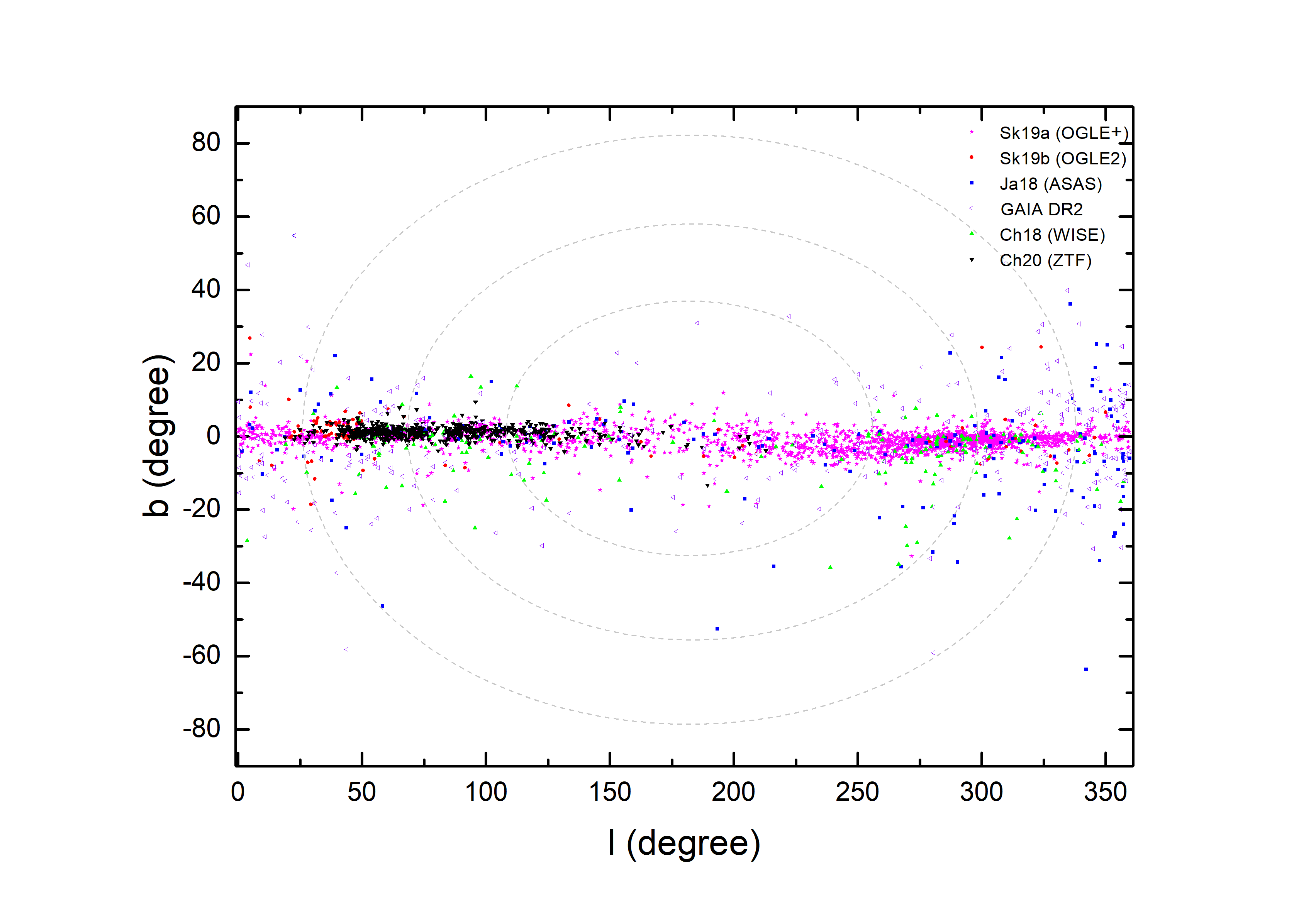
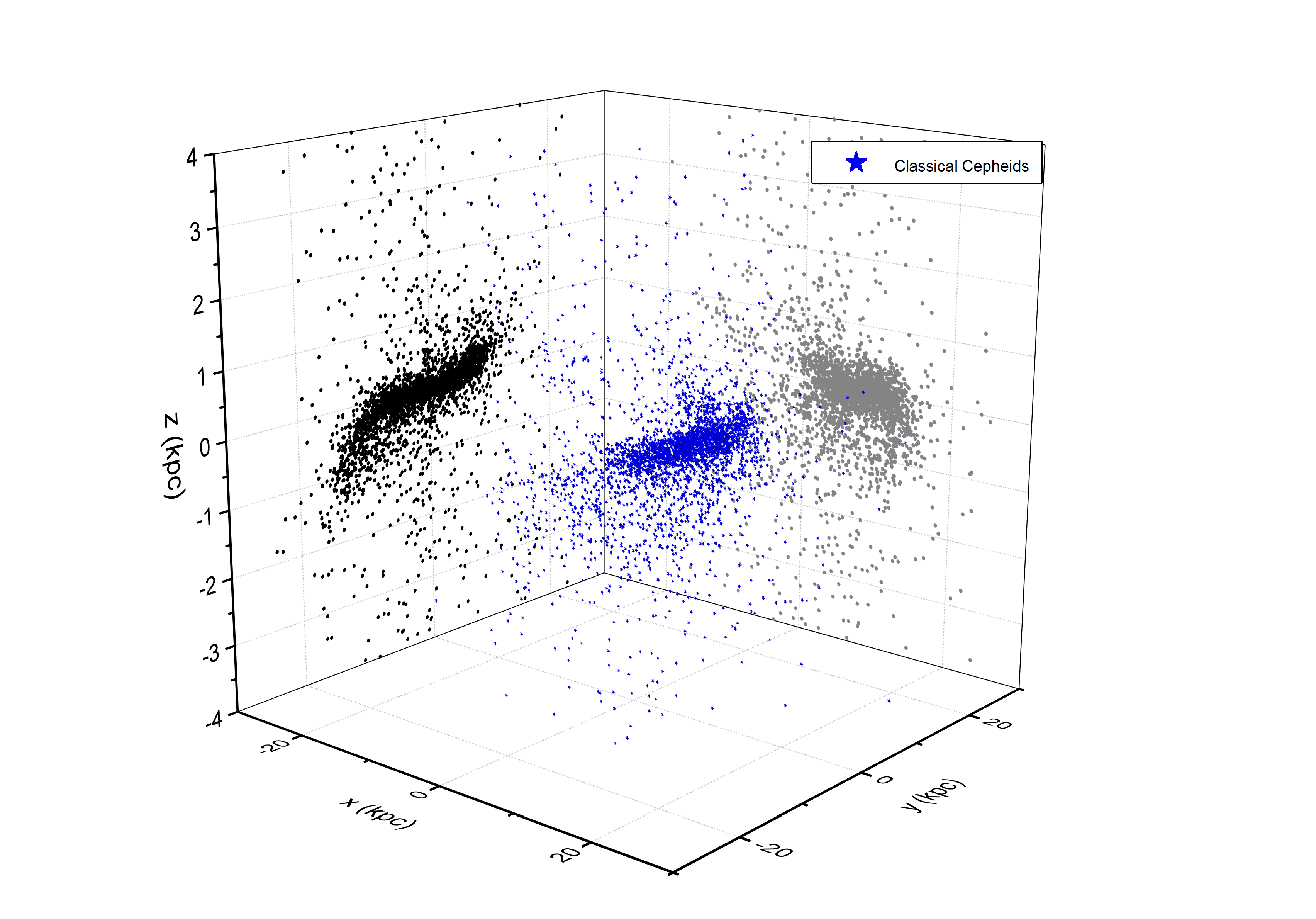
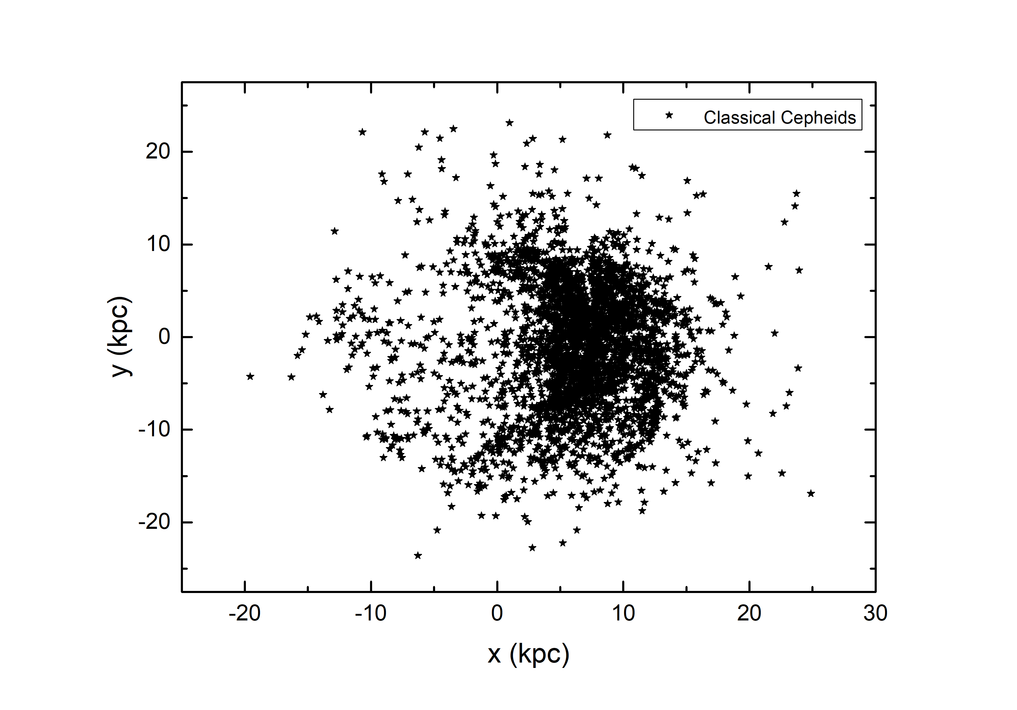
We collected our sample from several classical Cepheid catalogs as follows: the All-Sky Automated Survey for Supernovae (ASAS-SN) Variable stars catalog (Shappee et al. 2014; Jayasinghe et al. 2018), the classical Cepheids sample by Skowron et al. (2019a, b) basically from the Optical Gravitational Lensing Experiment (OGLE) (Udalski et al. 2015; Udalski et al. 2018), classical Cepheids from the European Space Agency (ESA) mission Gaia (Gaia Collaboration 2016, 2018; Ripepi et al. 2019), and the classical Cepheids catalog by Chen et al.(2019) from the Wide-field Infrared Survey Explorer (WISE) (Wright et al. 2010). We added new classical Cepheids identified from the Zwicky Transient Facility (ZTF) catalog (Bellm et al. 2019) by Chen et al.(2020). We made a cross-match of all the Cepheids from different catalogs in order to remove multiple entries. Then, we selected Cepheids which have mid-infrared ( and bands) magnitudes from the All WISE catalogue. We calculated heliocentric distances () based on the relations given in Wang et al. (2018) with and bands, and took average values for each Cepheid (also see Skowron et al. (2019a) for same calculation method). Recently, it has been discussed that distances derived from mid-infrared period-luminosity relations are more accurate than distances obtained from parallaxes (e.g., Mrz et al. 2019). After deriving distances, we keep classical Cepheids with kpc, and we have 3483 classical cepheids (Galactic longitude () and latitude () distributions are shown in the upper left panel of Figure 1): 2223 of them from Skowron et al. (2019a, b)(magenta stars and red circles), 160 from ASAS-SN catalog (blue squares), 303 from Gaia catalog (open Violet left triangles), 167 from Chen et al.(2019) (green triangles), 618 of them are from Chen et al.(2020) (black triangles).
The spatial distributions are shown in the Figure 1, and all distributions show the clear Galactic warp which is reported by Skowron et al. (2019a, b) and Chen et al.(2019). The 3D positions of Cepheids and galactocentric distances () in the Cartesian coordinate system are calculated as , , and , where is the distance from the Sun to the Galactic center, and the recent most accurate value, kpc (GRAVITY collaboration et al. 2018), is adopted. The projection of galactocentric distance on the Galactic plane () is as follows,
| (1) |
3 Modeling the rotation curve
3.1 The halo model
The rotation velocity at a radius from the center of an axisymmetric mass distribution is related to the total gravitational potential within and mass (at ),
| (2) |
where and are the gravitational potential and gravitational constant, respectively. If we consider the bulge, thin disk, thick disk and dark matter halo for the Galactic potential, which for the respective contributions are and ,
| (3) |
and velocity contributions to the RC from different components are given by,
| (4) |
The Navarro-Frenk-White (NFW) model (Navarro et al. 1996, 1997) which is derived from the simulations in the CMD scenario of galaxy formation has been widely used for modeling the dark matter halo (e.g., Sofue 2012; Wang et al. 2018). We assume that density distributions of all stellar components are well-known, and the velocity contribution of the dark matter halo is fitted by searching for the best-parameters by using the Markov Chain Monte Carlo method. For the fitting model, the Miyamoto-Nagai potential model (Miyamoto & Nagai 1975) and a spherical Plummer potential (Plummer 1911) are used for the thin/thick disks and bulge, respectively. We take the parameter values of the enclosed mass, the scale length, and the scale height from the model I of Pouliasis et al.(2017).
The NFW dark matter density profile is described as,
| (5) |
where , and is taken for the Hubble constant. The quantity of is the characteristic overdensity of the halo. Here, is the scale radius, where is so-called concentration parameter, and is the virial radius. is related to the virial mass as (see Navarro et al. (1996, 1997) for more details). In the next subsections, the rotation curves from different kinematical models and fitting results are discussed.
3.2 The rotation curve from proper motions
After measuring the proper motion of the star and setting the solar rotation speed as (Mrz et al. 2019), then assuming a circular orbit for the Cepheid, the following formula gives the rotation velocity (Gnaciski 2019),
| (6) |
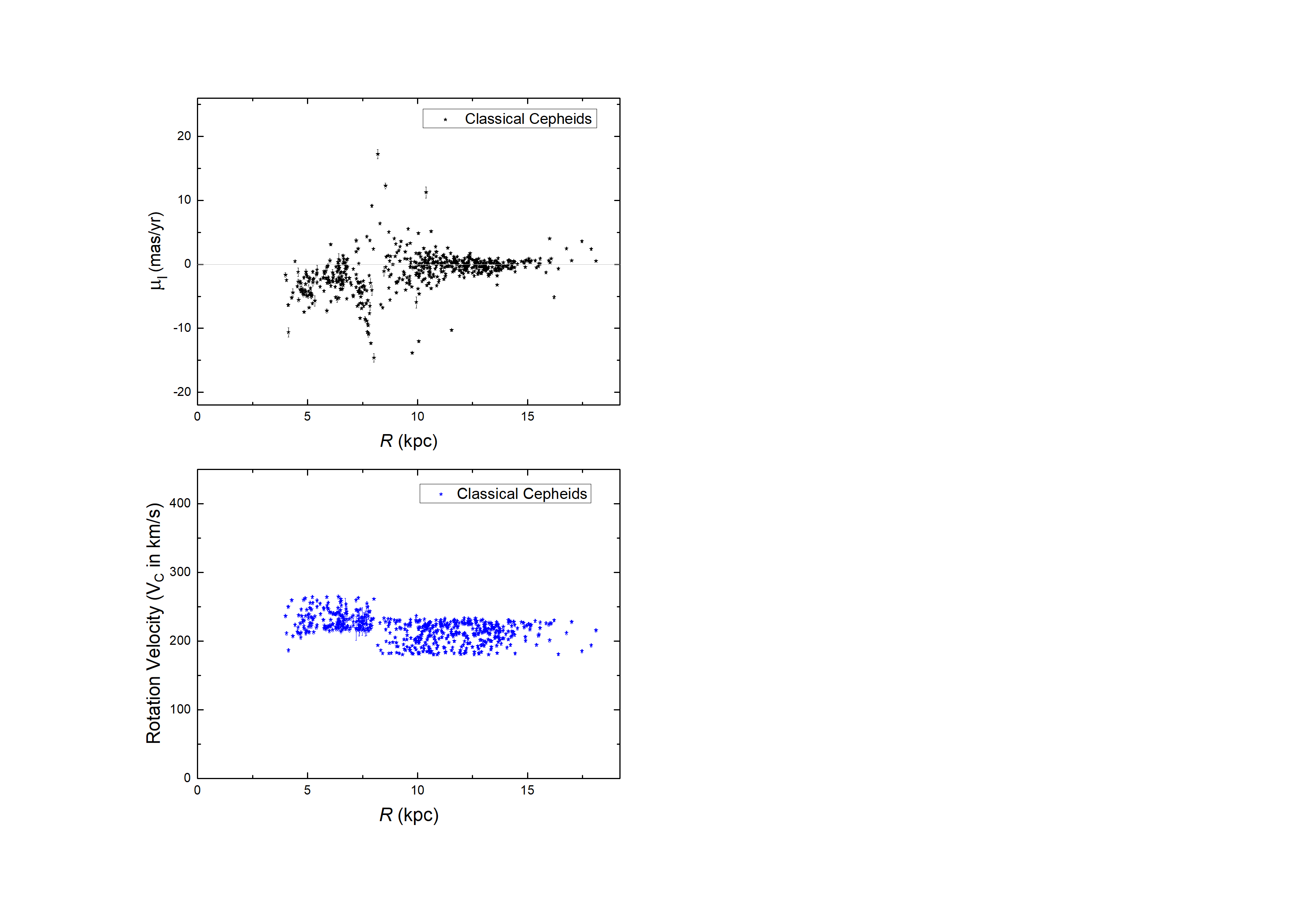
where the transverse velocity , and is the proper motion in the Galactic longitude (multiplied by ). The stars with kpc are excluded, and unphysical velocities caused by small or negative denominators are removed (see Gnaciski (2019) for the same selection criterion), so only 591 classical Cepheids are left from whole classical Cepheids for this kinematical modeling. Among our sample, there are 168, 324 and 411 classical Cepheids distributed in the Galactocentric range of kpc, kpc and kpc, respectively. Figure 2 shows and the calculated rotation velocities of 591 classical Cepheids. More than 98% of have uncertainties less than 0.2 , and this leads to small uncertainties in the rotation velocity calculation. The number of analyzed classical Cepheids in this work is about twice that used in Gnaciski (2019), and we have more stars in the outer disc which is helpful to improve the accuracy of the RC measurement.
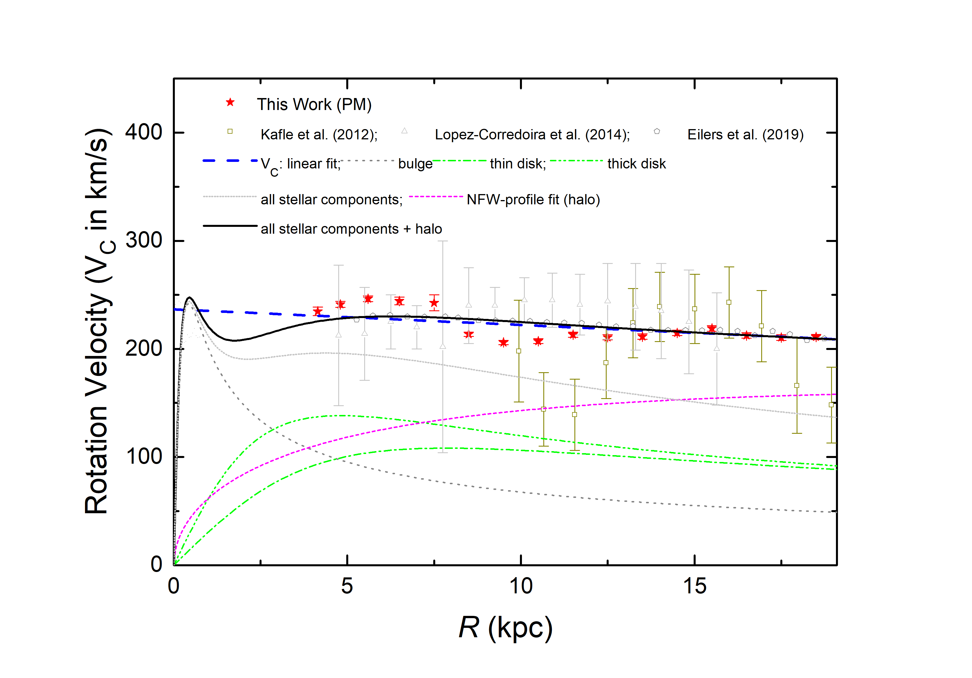
Figure 3 shows the rotation velocity distribution from kpc and 19 kpc (see Table 1 for the values), and the linear function fitted from it is,
| (7) |
This yields a gently declining rotation curve with a small gradient of () , and indicates the rotation velocity at the position of the Sun as . By fixing the contributions of baryonic components of the Galaxy (see model I of Pouliasis et al.(2017)), we estimated the mass and the properties of the Milky Way’s dark matter halo with the NFW profile (fitted results in Figure 3), and we derived , corresponding to a viral radius kpc. We obtained the concentration of and a scale radius of kpc. The indicated characteristic density is , and dark matter density at the location of the Sun is GeV .
3.3 The rotation curve from 3D velocity vector
The rotation velocity can also be determined from the 3D velocity vector if the three quantities of radial velocity and proper motions are available. Reid et al. (2009) described the calculation formulas of stellar motions by using radial velocity () and proper motions, which we adopt here: –velocity component toward the Galactic center, –velocity component along with the Galactic rotation, –toward the North Galactic pole. The optimizing model of , where and are the Sun’s rotation velocity and fitted parameter, is adopted for deriving rotation velocities (see Reid et al. (2009) for more details). For the peculiar (noncircular) solar motions with respect to the local standard of rest, the values of , and are taken from Schnrich et al. (2010).
The proper motions of the sample are obtained from the Gaia DR2, and the radial velocities are derived by cross-matching with Gaia DR2 and LAMOST DR6 data (e.g., Zhao et al. 2006, 2012). We excluded five Cepheids known in the binary systems, and we put extra constraints of kpc and radial velocity uncertainty to remove 11 objects in order to reduce uncertainties. It is well known that the radial velocity uncertainty may be larger for a single star when it’s measured near the pulsation phase (Stibbs 1955). However, the uncertainties of variable stars caused by the pulsation need further investigations, and it may not clearly affect the statistical result (see Ablimit & Zhao 2017). For the 3D velocity model, we have 1078 classical Cepheids: 836 of them from Skowron et al. (2019a,b), 55 from ASAS-SN catalog, 73 from Gaia DR2 Cepheids catalog, 22 from Chen et al.(2019), and 92 of them are from Chen et al.(2020). Among our sample, there are 47, 165, 377 and 659 classical Cepheids distributed in the Galactocentric range of kpc, kpc, kpc and kpc, respectively. In this work, the farest distance up to 19 kpc, simply because no star satisfies the criterion to model beyond 19 kpc. The radial velocities of 1043 stars are derived from the Gaia DR2 catalog while 35 of them obtained from LAMOST DR6.
There are likely some objects in 1078 star sample, which may be members of binary systems (and unrecognized with incorrect astrometric solutions) or categorized erroneously as classical Cepheids which as such and may actually be another type of variable. There are also some classical Cepheids with observed velocity components about 4 ( is dispersion of residuals) larger than the mean. Considering these possibilities and uncertainties, we selected 963 classical Cepheids from 1078 stars as the cleaned sample, and derived rotation velocities of the cleaned sample are shown in Table 1. The measured RCs from the cleaned sample and all 1078 sample can be fitted by the same linear function.
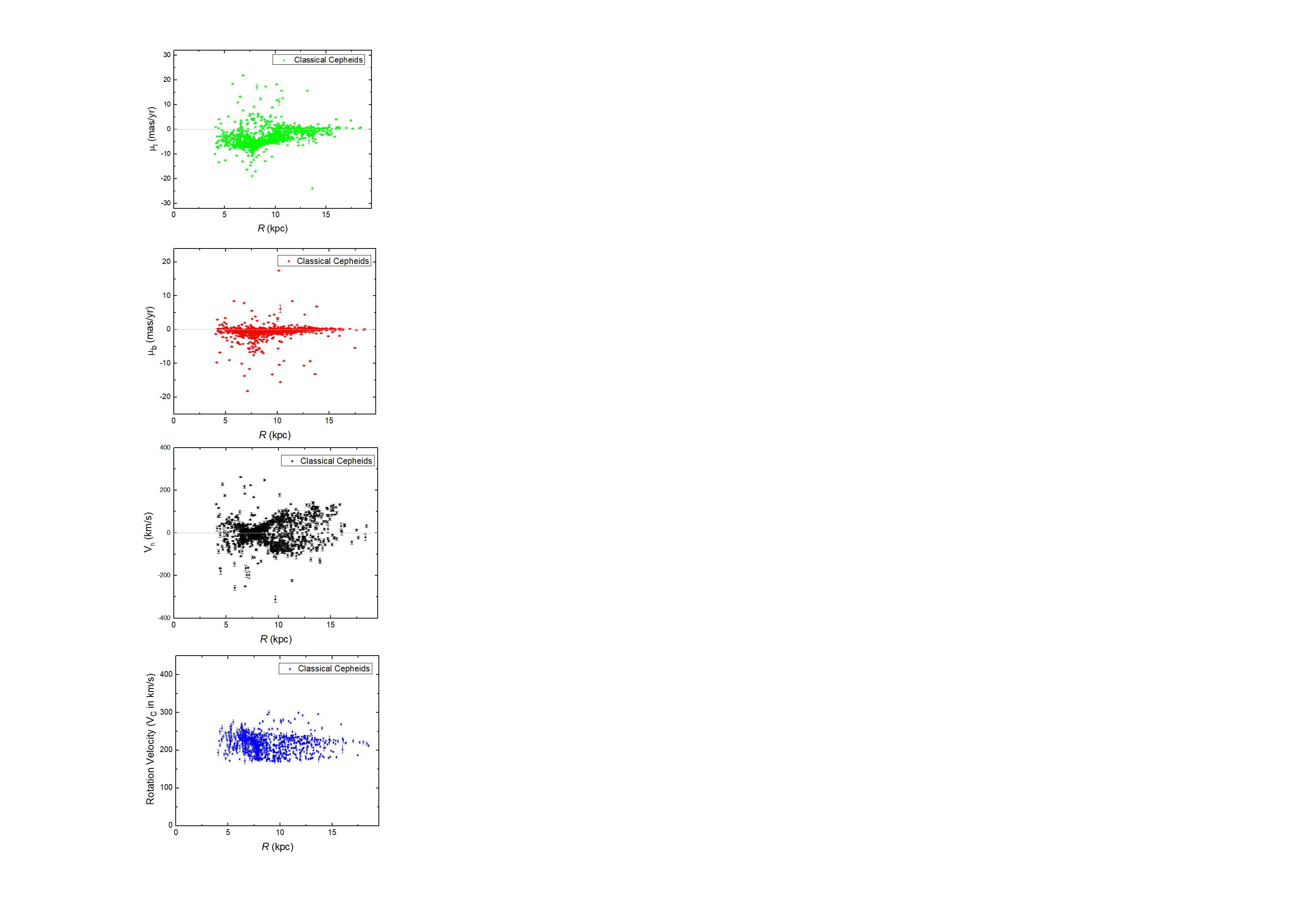
The distributions of , , and rotation velocities are given in Figure 4. The rotation curve from the 3D velocity vector (Figure 5) is well approximated by the following linear function,
| (8) |
The rotation curve from this method is gently decreasing with a derivative of () . The slope of the curve and rotation velocity at the location of the Sun () are in a good agreement with the results of Mrz et al. (2019), as about 70% of data points in the sample overlap with that of Mrz et al. (2019). However, there are more than 300 different stars in this work. In particular, our sample has more stars in the outer disc, which improves the accuracy of the RC, and is helpful to put more accurate constraint on the distribution of dark matter in the Milky Way. Comparing to the virial mass from the proper motion method, we derived a higher viral mass in this method, with a corresponding viral radius kpc. The resulted concentration and scale radius are and kpc, respectively. The estimated characteristic density and dark matter density at the location of the Sun are and GeV , respectively.
3.4 Comparison and discussion
There are 366 common classical Cepheids modeled in two methods, and different tracers are selected due to different criterion for different methods. The discrepancy of two methods’ results are within 10%. The most important advantage of our sample is the accuracy of the distances which have uncertainties at a level of 2-3%. We have small uncertainties in our results (see values of uncertainties in Table 1), however, only bootstrapping uncertainties without the systematic uncertainties are considered in this work (see Eilers et al. (2019) for analysis of the possible systematic uncertainties). The effect of the asymmetric drift is not considered in the calculation of this work due to the very small systematic uncertainty it causes (e.g., estimated as 0.28 by Kawata et al. 2018). Within 19 kpc, all systematic uncertainties added up (i.e. caused by uncertainties of distances, uncertainty of and the asymmetric drift etc.) only affect the RC measurement at a level. It is well known that the motions of stars are affected by Galactic substructures (e.g. Grand, Kawata & Cropper 2014; Bovy et al.2015; Kawata et al. 2018; Martinez-Medina et al. 2019). We did not use stars located at kpc in order to reduce the influence of other structures like the Galactic bar.
The slopes of the rotation curves from two methods are gently decreasing, as favored by the recent discoveries (e.g., Mrz et al. 2019; Eilers et al. 2019). They are not as flat as demonstrated in Sofue et al. (2009) and Reid et al. (2014), and it is not as steep as showed in Gnaciski (2019). This indicates that the dark matter content would not possibly so high or so low claimed in those previous works. The result (see the cross-point between the rotation curve of all stellar components and dark matter halo in Figure 3) from the proper motion method suggests that the dark matter halo dominates the Galactic rotation when kpc, and this is in good agreement with recent finding by Eilers et al. (2019). However, based on the 3D velocity method (as shown in Figure 5), the dark matter halo dominates the rotation velocity if kpc. The comparison of two velocity distributions from two methods give a same dip-like feature, there are a clear declining at the distance around 10 kpc, and this is consistent with the similar dip claimed by previous works (Sofue et al 2009; Kafle et al. 2012; McGauph 2018). However, there is no dip in the results of the cleaned sample with the 3D velocity method (Eilers et al. 2019).
The rotation velocity of the Sun found in the proper motion method is in good agreement with the results of some previous works (e.g., Bovy et al. 2012; Wegg et al. 2018). The Sun’s rotation velocity obtained from the 3D velocity method is, within uncertainties, consistent with the relatively higher values reported by Metezger et al. (1998), Reid et al.(2014), Kawata et al.(2018) and Mrz et al. (2019). The estimated virial masses from the two methods in this work are lower than the values () derived by Kpper et al. (2015), Bland-Hawthorn & Gerhard (2016), Watkins et al. (2019), Callingham et al.(2019) and Li et al. (2019). Within uncertainties, the viral masses in this work are in good agreement with the results of Bovy et al. (2012), Kalfe et al. (2012), Eadie et al. (2018), Eadie & Juri (2019), Eilers et al.(2019) and Cautun et al.(2019). The estimated mass by our 3D velocity method has very good agreement with the mean viral mass () derived by Karukes et al. (2019).
The estimated local dark matter densities from two methods including the uncertainties are consistent with the values of Weber & de Boer, (2010), Sofue (2012), Eilers et al. (2019) and Callingham et al.(2020). However, they are higher than the values ( GeV ) given by Gnaciski (2019), while they are lower than the estimated density ( GeV ) by Garbari et al.(2012) and ( GeV ) by Bienaym et al. (2014).
Effect of uncertainties of baryonic mass components. The estimation of the dark matter halo profiles rely on observational results of the baryonic mass components. Recently, de Salas et al.(2019) discussed that the dark matter density estimation is more sensitive to the uncertainties of the baryonic components rather than the uncertainties of the rotation velocities. They found a different uncertainty ( GeV ) of the dark matter density with the same velocities, and it is about 3 times of what Eilers et al. (2019) find. They also show that using different model such as the NFW dark matter profile and Einasto dark matter profile also gives a uncertainty of GeV . Comparing to the Galactic disc mass in some previous works (e.g., Smith et al. 2007), we took relatively higher masse for the Galactic (thin thick) disc from Pouliasis et al.(2017). Thus, we may underestimate the halo profiles. We examine it by taking a very simple example, and we run the model by using for the whole disc mass instead of (thin thick discs) as in this work from Model I of Pouliasis et al.(2017). We found that the dark matter density goes up to GeV when we reduce the baryonic mass of Galactic disc in the estimation modeling, and it is GeV higher than the value ( GeV ) derived from Model I of Pouliasis et al.(2017). This supports the statement given by de Salas et al.(2019). The future observational data may provide better constraints on the baryonic components222Note that previous works made important progress in modeling the baryon budget of Galactic disc and its uncertainties (e.g., Flynn et al. 2006; Bovy & Rix 2013).
Interestingly, the density derived from our 3D velocity method is basically consistent with the estimated dark matter density by de Salas et al.(2019) which is in a range of GeV . Our local dark matter density estimated from 3D velocity method is in very good agreement with the local dark matter density ( GeV ) inferred from fitting models to the Gaia DR2 Galactic rotation curve and other data (Cautun et al. 2019).
4 Conclusion
We have analyzed 3483 classical Cepheids selected from thousands of classical Cepheids identified by several survey projects (e.g., OGLE, ASAS-SN, Gaia, WISE and ZTF), and constructed the rotation velocity distribution of the Milky Way between the Galactocentric distance 4 kpc and 19 kpc by using two different methods. The distances of these classical Cepheids have the typical uncertainties of (which is crucial in the analysis of the rotation curve), and 3D spatial distributions show a vary clear Galactic warp feature claimed by previous works (see the section 2). 591 and 1078 classical Cepheids have been analyzed by using the proper motion and 3D velocity methods, and most of observed uncertainties of proper motions and radial velocities are less than 0.2 and 20 , respectively. This represents the largest classical Cepheid sample analyzed to date. We apply the NFW profile approach to simulate the dark matter content of the Milky Way. Our main findings are,
-
1.
The different methods or/and different sample would give different results in some extent. The uncertainties of baryonic components also have important role in the estimation of dark matter profiles. The result of the proper motion method shows that the dark matter halo is main contributor to the Galactic rotation when the distance kpc, while the 3D velocity modeling demonstrates that the Galactic rotation curve is dominated by the dark matter halo at kpc. The rotation curve constructed by both method are gently declining. The rotation curve from 3D velocity method is decreasing more gently with a derivative of () . The rotation velocity at the position of the Sun (() ) obtained from the 3D velocity method is about faster than the rotation velocity of the Sun derived from the proper motion method.
-
2.
The best-estimation with the NFW profile based on the rotation curve of the 3D velocity method generates a higher viral mass () with the corresponding radius of kpc and concentration of . At the same time, the predicted local dark matter density ( GeV ) is also higher than the estimated value from the proper motion modeling.
| Proper motion method | 3D velocity method | ||||
|---|---|---|---|---|---|
| R (kpc) | — | R (kpc) | |||
| 4.2 | 234.11 | 3.96 | 4.56 | 230.15 | 7.15 |
| 4.8 | 241.24 | 2.75 | 5.32 | 234.93 | 8.01 |
| 5.6 | 246.45 | 2.61 | 6.11 | 237.41 | 5.97 |
| 6.5 | 244.43 | 3.49 | 6.97 | 236.21 | 4.67 |
| 7.5 | 242.69 | 7.35 | 7.78 | 234.02 | 3.77 |
| 8.5 | 213.65 | 1.91 | 8.59 | 232.51 | 2.68 |
| 9.5 | 206.04 | 2.03 | 9.33 | 231.42 | 2.17 |
| 10.5 | 207.26 | 2.21 | 10.11 | 231.61 | 1.99 |
| 11.5 | 213.31 | 2.39 | 10.88 | 229.08 | 1.95 |
| 12.5 | 210.75 | 2.37 | 11.67 | 226.93 | 2.04 |
| 13.5 | 211.49 | 2.38 | 12.36 | 226.61 | 1.55 |
| 14.5 | 214.88 | 2.49 | 13.04 | 225.63 | 2.11 |
| 15.5 | 219.08 | 2.58 | 13.86 | 226.36 | 1.61 |
| 16.5 | 212.45 | 2.49 | 14.61 | 225.87 | 2.21 |
| 17.5 | 210.62 | 2.62 | 15.42 | 226.13 | 2.09 |
| 18.5 | 211.14 | 2.42 | 16.26 | 223.29 | 2.56 |
| 17.04 | 219.46 | 0.30 | |||
| 17.87 | 210.68 | 2.72 | |||
| 18.62 | 216.15 | 4.76 |