Testing Modified Gravity theory (MOG) with Type Ia Supernovae, Cosmic Chronometers and Baryon Acoustic Oscillations

Abstract

We analyse the MOdified Gravity (MOG) theory, proposed by Moffat, in a cosmological context. We use data from Type Ia Supernovae (SNe Ia), Baryon Acoustic Oscillations (BAO) and Cosmic Chronometers (CC) to test MOG predictions. For this, we perform $\chi^{2}$ tests considering fixed values of $H_{0}$ and $V_{G}$, the self-interaction potential of one of the scalar fields in the theory. Our results show that the MOG theory is in agreement with all data sets for some particular values of $H_{0}$ and $V_{G}$, being the BAO data set the most powerful tool to test MOG predictions, due to its constraining power.

I Introduction

The failure of Newton’s theory of Gravitation to successfully predict the motion of stars within galaxies and of galaxies in galaxy clusters was first reported by Oort Oort (1932) and Zwicky Zwicky (1937). Later observations of rotation curves in spiral galaxies Rubin et al. (1978, 1980) also pointed towards the same direction, namely: by assuming General Relativity (or its Newtonian counterpart) as the theory of gravity, the visible matter cannot account for the shape of the rotation curves. To solve this discrepancy, a component of non-luminous matter has been postulated. More recently, observations of astrophysical objects over a large range of mass and spatial scales (such as, for example, galaxy clusters, spiral and dwarf galaxies) Tyson et al. (1998); Hasselfield et al. (2013); Osato et al. (2018); Planck Collaboration et al. (2016); Sakamoto et al. (2003); Xue et al. (2008); Kafle et al. (2014); Iocco et al. (2015) have also shown the need for including a dark component of matter if the assumption of General Relativity as the theory of gravity holds.

As a consequence, one of the main ingredients of the standard cosmological model ($\Lambda$CDM) is a component of matter that does not couple to the electromagnetic field but can be detected via its gravitational interactions. In this way, this model is able to explain type Ia Supernovae data Scolnic et al. (2018), the Cosmic Microwave Background (CMB) power spectra Planck Collaboration et al. (2018), data from Baryon Acoustic Oscillations Ross et al. (2015); Alam et al. (2017); Abbott et al. (2018) as well as the formation of large scale structures Nuza et al. (2013). However, there is something missing in this picture, namely, the nature of this dark matter is currently unknown and none of the proposed candidates has been detected yet in the laboratory, despite numerous dedicated experimental efforts Schumann (2019).

An alternative to explain the mismatch between the data and the predictions of the current theory of gravity relies on a modification of the latter. In this regard, a first attempt was introduced by Milgrom in 1983 Milgrom (1983); the Modified Newtonian Dynamics (MOND) is a phenomenological proposal that follows from observations of galaxy rotation curves and the Tully-Fisher relation. More recently, in 2004, Bekenstein proposed a relativistic version of this theory named TeVeS Bekenstein (2004). One of the main unsolved issues of this theory is that it is not able to explain simultaneously the rotation curve of galaxies and the strong lensing effect, as well as the observations of the Bullet cluster Clowe et al. (2006a). Finally, in 2006, Moffat formulated the MOdified Gravity (MOG) theory in which one massive vector field and three scalar fields are added to the gravitational sector of the theory Moffat (2006). Moreover, this theory can predict successfully the motion within globular clusters, and clusters of galaxies Moffat and Toth (2008); Moffat and Rahvar (2014); Moffat and Zhoolideh Haghighi (2017) as well as the rotation curves of spiral and dwarf galaxies Moffat and Rahvar (2013); Zhoolideh Haghighi and Rahvar (2017). Nevertheless, some of us recently showed that the MOG theory is not able to explain the observed rotation curve of the Milky Way Negrelli et al. (2018). Moreover, when analyzing the Bullet cluster data Clowe et al. (2006b), there are different claims in the literature: some authors affirm that MOG cannot account for them Clowe et al. (2006a) while others hold that its predictions can fit data from both the Bullet and the Train Wreck merging clusters Brownstein and Moffat (2007); Israel and Moffat (2016). Additionally, it has been suggested that this theory is not compatible with the gas profile obtained from X-ray measurements and the strong-lensing properties of well-known galaxy clusters Nieuwenhuizen et al. (2018). However, in Ref Moffat and Zhoolideh Haghighi (2017) the authors show the opposite. On the other hand, as a consequence of the detection of a neutron star merger followed by its electromagnetic counterpart by the LIGO experiment, theories where the difference between the velocity of gravitational waves and the speed of light is significant, are ruled out Boran et al. (2018). However, Green et al. Green et al. (2018) pointed out that this is the case for bi-metric theories such as MOND and TeVeS, but not for MOG. In summary, the controversy about the compatibility of the MOG theory predictions with observational data at different scales is not yet settled.

On the other hand, it is well known that type Ia supernovae data have led to the discovery of the current accelerated expansion of the Universe Schmidt et al. (1998). However, there is no agreement within the scientific community about the physical mechanism responsible for this phenomenon. The simplest candidate is the one adopted by the $\Lambda$CDM model, namely, to include a cosmological constant in Einstein equations. Other proposals involve adding extra degrees of freedom to the Standard Model of Particles Tsujikawa (2011). Alternatively, the extra degrees of freedom can be added to the gravitational sector of the theory. In this regard, several alternative theories of gravity have been considered De Felice and Tsujikawa (2010), being MOG a particular case of such kind of theories. In summary, MOG offers an alternative to both the dark matter and dark energy ingredients of the standard cosmological model.

In this work, we focus on the predictions of the MOG theory on cosmological scales. In order to test its predictions, we consider data from Supernovae type Ia, Baryon Acoustic Oscillations and Cosmic Chronometers. We use $\chi^{2}$ tests to carry out the comparison between the mentioned data sets and the theoretical predictions. For this, we consider two fixed values $H_{0}$ (the one inferred from local data and the one obtained from the CMB data) and several values of $V_{G}$, the self-interaction potential of the scalar field that represents the gravitational constant.

In Section II, we briefly characterize the main aspects of the MOG theory at cosmological scales, analyzing the Friedmann equations and the expressions of the scalar fields of the theory. In Section III, we describe in detail the data sets that are used to test the predictions of the theory. Results of the comparison between the predictions of the MOG theory and each data set considered in this paper are shown and discussed in Section IV. Finally we present our conclusions in Section V.

II Cosmological background evolution of the MOG theory

In this section we summarize the main aspects of the MOG theory. In order to account for the effects that in the standard cosmological model are produced by dark matter and dark energy, this theory introduces a massive vector field $\phi^{\mu}$ and three scalar fields which are the following: i) $G$, the gravitational coupling strength, which is promoted to a scalar field; ii) $\mu$, which corresponds to the mass of the vector field; and iii) $\omega$, which describes the coupling strength between the vector field and matter. The gravitational and vector field $\phi^{\mu}$ actions are characterized by:

$$S_{G}=\frac{1}{16\pi}\int\frac{1}{G}\left({\it R}+2\Lambda\right)\sqrt{-g}~{}d^{4}x,$$ (1)

$$S_{\phi} = \frac{1}{4\pi}\int\omega\Big{[}\frac{1}{4}{\bf\it B^{\mu\nu}B_{\mu\nu}}-\frac{1}{2}\mu^{2}\phi_{\mu}\phi^{\mu}$$ (2)

$$+ V_{\phi}(\phi_{\mu}\phi^{\mu})\Big{]}\sqrt{-g}~{}d^{4}x,$$

while the scalar fields action is given by:

$$S_{S}= \int\frac{1}{G}\Big{[}\frac{1}{2}g^{\alpha\beta}\biggl{(}\frac{\nabla_{\alpha}G\nabla_{\beta}G}{G^{2}}+\frac{\nabla_{\alpha}\mu\nabla_{\beta}\mu}{\mu^{2}}+\nabla_{\alpha}\omega\nabla_{\beta}\omega\biggr{)}$$ (3)

$$+\frac{V_{G}(G)}{G^{2}}+\frac{V_{\mu}(\mu)}{\mu^{2}}+V_{\omega}(\omega)\Big{]}\sqrt{-g}~{}d^{4}x,$$

being $B_{\mu\nu}$ the Faraday tensor of the vector field ($B_{\mu\nu}=\partial_{\mu}\phi_{\nu}-\partial_{\nu}\phi_{\mu}$) and $V_{\phi}(\phi_{\mu}\phi^{\mu})$, $V_{G}(G)$, $V_{\omega}(\omega)$ and $V_{\mu}(\mu)$, the self-interaction potentials associated with the vector field and the scalar fields. Finally, $\nabla_{\nu}$ is the covariant derivative with respect to the metric $g_{\mu\nu}$.

The Friedmann equations for this theory can be obtained assuming an homogeneous and isotropic space-time which can be described by Friedmann-Lemaître-Robertson-Walker (FLRW) line element ($ds^{2}=dt^{2}-a^{2}(t)[(1-kr^{2})^{-1}dr^{2}+r^{2}d\Omega^{2}])$ Moffat and Toth (2009):

$$H^{2}+ \frac{k}{a^{2}}=\frac{8\pi G\rho}{3}-\frac{4\pi}{3}\biggl{(}\frac{\dot{G}^{2}}{G^{2}}+\frac{\dot{\mu}^{2}}{\mu^{2}}+\dot{\omega}^{2}-\frac{1}{4\pi}G\omega\mu^{2}\phi_{0}^{2}\biggr{)}$$ (4)

$$+\frac{8\pi}{3}\biggl{(}\frac{\omega GV_{\phi}}{4\pi}+\frac{V_{G}}{G^{2}}+\frac{V_{\mu}}{\mu^{2}}+V_{\omega}\biggr{)}+\frac{\Lambda}{3}+H\frac{\dot{G}}{G},$$

$$\frac{\ddot{a}}{a}= -\frac{4\pi G}{3}(\rho+3p)+\frac{8\pi}{3}\biggl{(}\frac{\dot{G}^{2}}{G^{2}}+\frac{\dot{\mu}^{2}}{\mu^{2}}+\dot{\omega}^{2}-\frac{1}{4\pi}G\omega\mu^{2}\phi_{0}^{2}\biggr{)}$$ (5)

$$+\frac{8\pi}{3}\biggl{(}\frac{\omega GV_{\phi}}{4\pi}+\frac{V_{G}}{G^{2}}+\frac{V_{\mu}}{\mu^{2}}+V_{\omega}\biggr{)}+\frac{\Lambda}{3}$$

$$+H\frac{\dot{G}}{2G}+\frac{\ddot{G}}{2G}-\frac{\dot{G}^{2}}{G^{2}},$$

these equations can be combined to obtain a differential equation for the scale factor $a$:

$$\frac{\ddot{a}}{a}+\frac{\dot{a}^{2}}{2a^{2}}+\frac{k}{2a^{2}}= -4\pi Gp+2\pi\biggl{(}\frac{\dot{G}^{2}}{G^{2}}+\frac{\dot{\mu}^{2}}{\mu^{2}}+\dot{\omega}^{2}-\frac{G\omega\mu^{2}\phi_{0}^{2}}{4\pi}\biggr{)}$$ (6)

$$+4\pi\biggl{(}\frac{\omega GV_{\phi}}{4\pi}+\frac{V_{G}}{G^{2}}+\frac{V_{\mu}}{\mu^{2}}+V_{\omega}\biggr{)}$$

$$+\frac{\Lambda}{2}+\frac{\ddot{G}}{2G}-\frac{\dot{G}^{2}}{G^{2}}+H\frac{\dot{G}}{2G}.$$

In this work, like in the standard cosmological model, we model the baryonic matter as a pressureless dust such that $p=0$ and $w=p/\rho=0$. On the other hand, it has been discussed in Section I that in the MOG theory it is not necessary to include dark matter to explain astrophysical and cosmological observations. Therefore, only baryonic matter will be included in the modified Friedmann Equations. However, given that the matter density does not appear in Eq. 6, the evolution of the cosmic scale factor and, in consequence, of the Hubble parameter will depend only on the pressure of the baryonic matter which in the case of pressureless dust is zero.

On the other hand, the equation of motion for the scalar fields can be derived from Eq. 3:

$$\ddot{G} +3H\dot{G}-\frac{3}{2}\frac{\dot{G}^{2}}{G}+\frac{G}{2}\biggl{(}\frac{\dot{\mu}^{2}}{\mu^{2}}+\dot{\omega}^{2}\biggr{)}-\frac{3}{G}V_{G}-V^{\prime}_{G}$$ (7)

$$+G\Big{[}\frac{V_{\mu}}{\mu^{2}}+V_{\omega}\Big{]}+\frac{G}{8\pi}\Lambda-\frac{3G}{8\pi}\biggl{(}\frac{\ddot{a}}{a}+H^{2}+\frac{k}{a^{2}}\biggr{)}=0,$$

$$\ddot{\mu}+3H\dot{\mu}-\frac{\dot{\mu}^{2}}{\mu}-\frac{\dot{G}}{G}\dot{\mu}+\frac{G\omega\mu^{3}\phi^{2}_{0}}{4\pi}+\frac{2}{\mu}V_{\mu}-V^{\prime}_{\mu}=0,$$ (8)

$$\ddot{\omega}+3H\dot{\omega}-\frac{\dot{G}}{G}\dot{\omega}+\frac{1}{8\pi}G\mu^{2}\phi^{2}_{0}-\frac{GV_{\phi}}{4\pi}-V^{\prime}_{\omega}=0,$$ (9)

where $V^{\prime}_{G}=\frac{dV_{G}}{dG}$, $V^{\prime}_{\mu}=\frac{dV_{\mu}}{d\mu}$ and $V^{\prime}_{\omega}=\frac{dV_{\omega}}{d\omega}$.

In Section I, we pointed out that the MOG theory might explain the late acceleration in the expansion of the Universe, even if Einstein’s cosmological constant is set to 0. The reason for this is that the equation of state associated to the self-interaction potentials $V_{G}$, $V_{\omega}$, $V_{\phi}$ and $V_{\mu}$ is of the form $w_{V}=-1$ Moffat and Toth (2007, 2013). One of the goals of this work is to test if the MOG theory can supply the role of the dark energy, therefore we set $\Lambda=0$. On the other hand, as in the standard cosmological model, we consider a flat universe, i.e. $k=0$.

As regards the self-interaction potentials, the most simple assumption would be to take them all equal to 0. However, it has been shown that in order to describe properly cosmological quantities such as the age and evolutionary stages of the Universe Toth (2010); Jamali and Roshan (2016), and redshift space distortion (RSD) data Jamali et al. (2018), $V_{G}$ must be different from $0$. Furthermore, previous studies of the MOG theory in the cosmological context Moffat and Toth (2007, 2013) consider $V_{G}>0$. Therefore, in this paper, we consider MOG models with $V_{G}=0$ and $V_{G}\neq 0$ to test different data sets in the cosmological context (see section IV). Also, we set $V_{\mu}=V_{\omega}=V_{\phi}=0$.

To find the expressions for $H(z)$, $G(z)$, $\mu(z)$ and $\omega(z)$, equations (6), (7), (8) and (9) need to be solved numerically with suitable initial conditions. We use the ones proposed in Ref.Moffat and Toth (2007):

$$t_{0} = 13.7\times 10^{9}~{}\mathrm{years},$$

$$a_{0} = c\,t_{0},$$

$$G_{0} = 6\,G_{N},$$

$$\mu_{0} = a_{0}^{-1},$$

$$\omega_{0} = 1/\sqrt{12},$$

$$\phi_{0} = 0,$$

$$\dot{a}_{0} = H_{0}\,a_{0},$$

$$\dot{G}_{0}=\dot{\mu}_{0}=\dot{\omega}_{0} = 0,$$

where $G_{N}$ refers to the Newton’s gravitational constant. The choices of $t_{0}$ and $a_{0}$, are the same as in the flat standard cosmological model. Besides, since there is no agreement within the scientific community about the reported value of $H_{0}$ (which is referred in the literature as the $H_{0}$ tension), we consider two different values for this parameter, namely the values inferred from local and CMB observations (see section IV for a detailed discussion of this choice). The solution of the MOG field equations in the spherically symmetric case (for details, see  Moffat and Toth (2009, 2013)) defines the scalar fields values, being $\mu_{0}$ the inverse of the scale of the Universe. On the other hand, the choice of $G_{0}$ is motivated by the following reason: an effective gravitational constant $G_{\rm eff}\approx 6\,G_{N}$ at the Yukawa distance $r=\mu^{-1}$ is compatible with the results coming from the test particle equation of motion expression, being $G_{\rm eff}\approx 20\,G_{N}$ at infinity. As a consequence, on superhorizon scales the present solution would be consistent with an Einstein-de Sitter cosmology without dark components Moffat and Toth (2007, 2013).

The integrated $G(z)/G_{0}$ can be seen in Fig 1. Also, as a result of the numerical integration, it follows that $\omega$ and $\mu$ are constants as a function of $z$. All these results are consistent with the ones obtained by Moffat & Toth in Moffat and Toth (2007). On the other hand, it follows from Fig. 1 that if $V_{G}=0$, the behaviour of $G(z)/G_{0}$ does not depend on the value assumed for $H_{0}$. Conversely, if the case with $V_{G}\neq 0$ is considered, different solutions are obtained when different values of $H_{0}$ are considered (see Fig. 1). An explanation for this behavior lies in the fact that, if $V_{G}\neq 0$, a term proportional to $\frac{V_{G}}{G^{2}}$ is added to Eq. 6.

Figure 1: $\frac{G(z)}{G_{0}}$ for MOG models with fixed values of $H_{0}$ (labeled in the figure in units of km s^-1 Mpc^-1) and $V_{G}$. $V_{G}^{M}=0.077\frac{G_{0}^{2}}{t_{0}^{2}}$ is the value suggested in Ref. Moffat and Toth (2007) which also analyses the MOG theory in the cosmological context.

III Observational constraints

In this section, we describe the data sets that we use to make the comparison with the predictions of the MOG theory.

III.1 Cosmic chronometers

The Cosmic Chronometer (CC) approach is very useful to track the Universe evolution. This method was proposed and implemented in Jimenez and Loeb (2002) and it allows to determine the Hubble parameter $H(z)$ from the following expression:

$$H(z)=\frac{-1}{1+z}\frac{dz}{dt}.$$ (10)

The method is based on the differential age evolution of old elliptical passive-evolving galaxies that formed at the same time but are separated by a small redshift interval. In this way, by measuring the age difference of those galaxies, the derivative $\frac{dz}{dt}$ can be measured from the ratio $\frac{\Delta z}{\Delta t}$.

Good candidates for cosmic chronometers are galaxies that have been formed early in the Universe, at high redshift ($z>2-3$), with large mass ($\mathcal{M}_{\rm stars}>10^{11}\mathcal{M}_{\odot}$), and which have not had any star formation ever since. In this way, if these galaxies are observed at later cosmic time, the age evolution of their stars can be used as a clock synchronized with the evolution of cosmic time. Spectroscopic surveys allow to obtain $dz$ with high accuracy. The main advantage of this method lies in the measurement of relative ages $dt$, which avoids the systematic effects that affect the determination of absolute ages. Moreover, the determination of $dt$ depends only on atomic physics and not on the integrated distance along the line of sight (redshift) which, in turn, is a function of the cosmological model.

In this paper, we consider the most recent and accurate estimates of $H(z)$ acquired through this method (see Table 1) to test the predictions of the MOG theory. Simon et al. Simon et al. (2005) used the GDDS catalogue Abraham et al. (2004) together with spectroscopic data from other galaxies Dunlop et al. (1996); Nolan et al. (2003); Spinrad et al. (1997); Treu et al. (1999, 2001, 2002) to obtain 9 determinations of $H(z)$ in the redshift range $0.09\leq z\leq 1.75$. Stern et al. Stern et al. (2010a) obtained high quality spectra from red galaxies and used them together with spectra from the SPICES Stern et al. (2001) and VVDS Le Fèvre et al. (2005) catalogues to obtain two measurements of $H(z)$ at $z=0.48$ and $z=0.88$. Moresco et al. Moresco et al. (2012) took a sample of 11,000 massive red galaxies from different catalogues Cimatti et al. (2002); Demarco et al. (2010); Eisenstein et al. (2001); Le Borgne et al. (2006); Lilly et al. (2009); Onodera et al. (2010); Rosati et al. (2009); Stern et al. (2010b); Strauss et al. (2002); Vanzella et al. (2008) to obtain 8 measurements of $H(z)$ within the redshift range $0.17<z<1.04$. Zhang et al. Zhang et al. (2014) obtained their results in the redshift interval $0.07\leq z\leq 0.28$ taking 17,832 red galaxies from the Sloan Digital Sky Survey Data Release Seven (SDSS DR7) Abazajian et al. (2009). Moresco Moresco (2015) considered spectroscopic data of 29 high redshift galaxies ($z>1.4$) Gobat et al. (2013); Kriek et al. (2009); Krogager et al. (2014); Onodera et al. (2012); Saracco et al. (2005) to obtain estimations of $H(z)$ at redshift $z=1.363$ and $z=1.965$. Moresco et al. Moresco et al. (2016) used data from the BOSS catalogue Dawson et al. (2013); Eisenstein et al. (2011) to obtain 5 measurements of $H(z)$ in the redshift range $0.38<z<0.48$.

$z$	$H(z)\ (\mathrm{km}\,\mathrm{s}^{-1}\,\mathrm{Mpc}^{-1})$	Reference
0.09	69 $\pm$ 12
0.17	83 $\pm$ 8
0.27	77 $\pm$ 14
0.4	95 $\pm$ 17
0.9	117 $\pm$ 23	Simon et al. (2005)
1.3	168 $\pm$ 17
1.43	177 $\pm$ 18
1.53	140 $\pm$ 14
1.75	202 $\pm$ 40
0.48	97 $\pm$ 62	Stern et al. (2010a)
0.88	90 $\pm$ 40
0.1791	75 $\pm$ 4
0.1993	75 $\pm$ 5
0.3519	83 $\pm$ 14
0.5929	104 $\pm$ 13	Moresco et al. (2012)
0.6797	92 $\pm$ 8
0.7812	105 $\pm$ 12
0.8754	125 $\pm$ 17
1.037	154 $\pm$ 20
0.07	69 $\pm$ 19.6
0.12	68.6 $\pm$ 26.2	Zhang et al. (2014)
0.2	72.9 $\pm$ 29.6
0.28	88.8 $\pm$ 36.6
1.363	160 $\pm$ 33.6	Moresco (2015)
1.965	186.5 $\pm$ 50.4
0.3802	83 $\pm$ 13.5
0.4004	77 $\pm$ 10.2
0.4247	87.1 $\pm$ 11.2	Moresco et al. (2016)
0.4497	92.8 $\pm$ 12.9
0.4783	80.9 $\pm$ 9

Table 1: $H(z)$ constraints obtained from the cosmic chronometers. The table shows the redshift of the measurement, the mean value and standard deviation of $H(z)$

in units of km s^-1 Mpc^-1 and the corresponding reference.

III.2 Supernovae type Ia

Type Ia Supernovae (SNe Ia) are among the most energetic events in the Universe. They are quite common, and are observed in different kind of galaxies. The extremely high luminosity of the supernovae makes them easily detectable by surveys. Most importantly, the homogeneity of their spectra and light curves makes them excellent candidates to be considered as standard candles.

The distance modulus of a supernova is given by,

$$\mu=25+5\log_{10}(d_{L}(z)),$$ (11)

being $d_{L}$ the luminosity distance that depends on the cosmological model and redshift $z$,

$$d_{L}(z)=(1+z)\int_{0}^{z}\frac{dz^{\prime}}{H(z^{\prime})}.$$ (12)

Then, it is possible to compare the theoretical distance modulus of the MOG theory with the modulus obtained from the SNe Ia data.

In this paper, we consider the Pantheon compilation Scolnic et al. (2018) of 1,048 SNe Ia in the redshift interval $0.01<z<2.3$. The observed distance modulus estimator for this compilation is given by

$$\mu=m_{B}-M+\alpha x_{1}+\beta c+\Delta_{M}+\Delta_{B},$$ (13)

where $\Delta_{M}$ is a distance correction based on the mass of the SNe Ia’s host-galaxy, and $\Delta_{B}$ is a distance correction based on predicted biases from simulations. Furthermore, $m_{B}$ is an overall flux normalization, $x_{1}$ and $c$ refer to the deviation from the average light-curve shape and the mean SNe Ia BV color, respectively. Finally, $M$ is the absolute B-band magnitude of a fiducial SNe Ia with $x_{1}=0$ and $c=0$. Parameter $\alpha$ represents the coefficient of the relation between luminosity and stretch; while $\beta$, the coefficient of the relation between luminosity and color.
For the Pantheon data compilation $\Delta_{M}$ is determined by:

$$\Delta_{M}=\gamma\times[1+e^{(-(m-m_{\rm step})/\tau)}]^{-1}$$ (14)

where $\gamma$ stands for a relative offset in luminosity; $m_{\rm step}$, a mass step for the split; and $\tau$, an exponential transition term in a Fermi function that describes the relative probability of masses being on one side or the other of the split. The last two ($m_{\rm step}$ and $\tau$) are obtained from different host galaxies samples (technicalities are described in Scolnic et al. (2018)) and $m$ is the host-galaxy mass. Finally, $\alpha$, $\beta$, $M$ and $\gamma$ account for nuisance parameters.

III.3 BAO

Before the formation of neutral hydrogen, photons and free electrons were coupled through Thomson scattering, generating accoustic waves in the primordial plasma. After recombination, matter and radiation decouples. The maximum distance the accoustic wave could travel defines a characteristic scale, named the sound horizon at the drag epoch $r_{d}$; this scale is imprinted in the distribution of matter in the Universe. Baryon Accoustic Oscillations (BAO) provide a standard ruler to measure cosmological distances. Different tracers of the underlying matter density field provide probes to measure distances at different redshifts.

Along the line of sight, the BAO signal directly constrains the Hubble constant $H(z)$ at redshift $z$. When measured in a redshift shell, it constrains the angular diameter distance $D_{A}(z)$,

$$D_{A}(z)=\frac{c}{(1+z)}\int_{0}^{z}\frac{dz^{\prime}}{H(z^{\prime})}.$$ (15)

To separate $D_{A}(z)$ and $H(z)$, BAO should be measured in the 2D correlation function, for which extremely large volumes are necessary. If this is not the case, a combination of both quantities can be measured as

$$D_{V}(z)=\left[(1+z)^{2}D_{A}^{2}(z)\frac{cz}{H(z)}\right]^{1/3}.$$ (16)

BAO have been measured with great precision using different observational probes. To measure the BAO scale from the clustering of matter, it is necessary to define a fiducial cosmology. Most of the distance constraints presented in Table 2 are multiplied by a factor $(r_{d}/r_{d}^{fid})$, which is the ratio between the sound horizon at the drag epoch to the same quantity computed in the fiducial cosmology. We take this ratio as a free parameter in the statistical analysis.

$z_{\rm eff}$	Value	Observable	Reference
$0.16$	$456\pm 27.0$ Mpc	$D_{V}$	Beutler et al. (2011)
$0.15$	$(664\pm 25.0)(r_{d}/r_{d}^{fid})$ Mpc	$D_{V}$	Ross et al. (2015)
$0.81$	$(1649.5\pm 66.0)(r_{d}/r_{d}^{fid})$ Mpc	$D_{A}$	Abbott et al. (2018)
$0.38$	$(1512\pm 33)(r_{d}/r_{d}^{fid})$ Mpc	$D_{M}$
$0.38$	$(81.2\pm 3.2)(r_{d}/r_{d}^{fid})$ km s-1 Mpc-1	$H$
$0.51$	$(1975\pm 41)(r_{d}/r_{d}^{fid})$ Mpc	$D_{M}$	Alam et al. (2017)
$0.51$	$(90.9\pm 3.3)(r_{d}/r_{d}^{fid})$ km s-1 Mpc-1	$H$
$0.61$	$(2307\pm 50)(r_{d}/r_{d}^{fid})$ Mpc	$D_{M}$
$0.61$	$(99.0\pm 3.4)(r_{d}/r_{d}^{fid})$ km s-1 Mpc-1	$H$
$0.44$	$(1716\pm 83.0)(r_{d}/r_{d}^{fid})$ Mpc	$D_{V}$
$0.6$	$(2221\pm 101.0)(r_{d}/r_{d}^{fid})$ Mpc	$D_{V}$	Kazin et al. (2014)
$0.73$	$(2516\pm 86.0)(r_{d}/r_{d}^{fid})$ Mpc	$D_{V}$
$1.52$	$(3843\pm 147.0)(r_{d}/r_{d}^{fid})$ Mpc	$D_{V}$	Ata et al. (2017)
$2.3$	$(1336\pm 45.7)(r_{d}/r_{d}^{fid})$ Mpc	$D_{H}$	Bautista et al. (2017)
$2.3$	$(5566\pm 317.2)(r_{d}/r_{d}^{fid})$ Mpc	$D_{M}$
$2.4$	$(1327.4\pm 53.0)(r_{d}/r_{d}^{fid})$ Mpc	$D_{H}$	du Mas des Bourboux et al. (2017)
$2.4$	$(5259.7\pm 250.5)(r_{d}/r_{d}^{fid})$ Mpc	$D_{M}$

Table 2: Distance constraints from BAO measurements of different observational probes. The table shows the redshift of the measurement, the mean value and standard deviation of the observable, the observable that is measured in each case and the corresponding reference.

In the following, we describe the observations used in this work. The large-scale correlation function of the 6dF Galaxy Survey (6dFGS) Beutler et al. (2011), which is obtained from a K-band selected galaxy subsample with redshifts, determines a value for the isotropic angular diameter distance $D_{V}$ at effective redshift, $z_{\rm eff}$ of 0.106. The same quantity at $z_{\rm eff}=0.15$ is computed in Ross et al. Ross et al. (2015), using the main sample of SDSS-DR7 galaxies, with measured redshifts, in combination with a reconstruction method to alleviate the effect of non-linearities on the BAO scale. The first year data release of the Dark Energy Survey Abbott et al. (2018) provides a measurement of the angular diameter distance $D_{A}$ at $z_{\rm eff}=0.81$, using the projected two point correlation function of a sample of over 1.3 million galaxies with measured photometric redshifts, distributed over a footprint of 1336 deg². The final galaxy clustering data release of the Baryon Oscillation Spectroscopic Survey Alam et al. (2017), provides measurements of the comoving angular diameter distance $D_{M}$ (related with the physical angular diameter distance by $D_{M}(z)=(1+z)D_{A}(z)$) and Hubble parameter $H$ from the BAO method after applying a reconstruction method, for three partially overlapping redshift slices centred at effective redshifts 0.38, 0.51, and 0.61. Using the WiggleZ Dark Energy Survey Kazin et al. (2014) and a reconstruction method, measurements of $D_{V}$ at effective redshifts of 0.44, 0.6, and 0.73 are provided. With a sample of 147000 quasars from the extended Baryon Oscillation Spectroscopic Survey (eBOSS) Ata et al. (2017) distributed over 2044 square degrees with redshifts $0.8<z<2.2$, a measurement of $D_{V}$ at $z_{\rm eff}=1.52$ is provided. The BAO can be also determined from the flux-transmission correlations in Ly$\alpha$ forests in the spectra of 157,783 quasars in the redshift range $2.1<z<3.5$ from the Sloan Digital Sky Survey (SDSS) data release 12 (DR12) Bautista et al. (2017). Measurements of $D_{M}$ and the Hubble distance (defined as $D_{H}=c/H(z)$) at $z_{\rm eff}=2.33$ are provided. From the cross-correlation of quasars with the Ly$\alpha$-forest flux transmission of the final data release of the SDSS-III du Mas des Bourboux et al. (2017), a measurement of $D_{M}$ and $D_{H}$ at $z_{\rm eff}=2.4$ can be obtained.

IV Results

In this section, we compare MOG cosmological predictions, explained in Section II, with the observational data described in Section III. We use $\chi^{2}$ tests to quantify the agreement between the theoretical results and the data. To proceed with the comparison, we define a fiducial model, that will be taken as a reference to analyze the predictions of the MOG models. It is well known that there is a tension between the value of $H_{0}$ obtained from the Cosmic Microwave Background (CMB)  Planck Collaboration et al. (2018) and the one inferred from local measurements  Riess et al. (2018). Therefore, we choose two $\Lambda$CDM models with fixed values of $H_{0}$ and the total matter density parameter $\Omega_{m}$ as follows:

• $\Lambda$CDM Model 1: $H_{0}=67.4$ km sec^-1 Mpc^-1 and $\Omega_{m}=0.315$; the values obtained by the Planck collaboration using CMB data Planck Collaboration et al. (2018).

• $\Lambda$CDM Model 2: $H_{0}=73.5$ km sec^-1 Mpc^-1 and $\Omega_{m}=0.298$; the values inferred from cepheids and type Ia supernovae in Refs. Riess et al. (2018) and Scolnic et al. (2018) respectively.

We perform separate statistical analyses for each data set, for which we test the predictions of the MOG theory for different values of $V_{G}$ and particular values of $H_{0}$ (namely, those of the fiducial models defined above). Results are shown in Tables 3, 4, 5 and 6 together with the corresponding $\tilde{\chi}^{2}_{5\sigma}$ value , for the number of data and free parameters considered in each case. Notice that $V_{G}^{M}=0.077G_{0}^{2}/t_{0}^{2}$ is the value suggested by Moffat and Toth (2007), who also analyze this theory in a cosmological context.

It follows from Section II that the theoretical prediction of the MOG theory for the scale factor evolution and its derived quantity $H(z)$ involves no free parameters. On the other hand, eq. (13) shows that the analysis of supernovae data involves several free parameters: the nuisance parameters and the absolute magnitude $M$. In all of the analyses done in this paper, we consider the absolute magnitude $M$ as a free parameter. Regarding the nuisance parameters, we consider two cases: i) fixed values given by the Pantheon compilation (Table 3) and ii) the nuisance parameters are allowed to vary (Table 4). The reason for this, is that the nuisance parameters given by the Pantheon compilation were obtained assuming a $\Lambda$CDM model for the theoretical predictions of the distance modulus and therefore it is not correct to assume a priori those values when analyzing an alternative cosmological model. Nevertheless, the obtained confidence intervals for the nuisance parameters are consistent with those given by the Pantheon compilation at 1$\sigma$ level. Therefore, the present analysis confirms the robustness of those parameters.

It can be noticed from Table 3 that only when $V_{G}=0$ is considered, the predictions of the corresponding MOG models are inconsistent with type Ia supernovae data at 5$\sigma$. Conversely, the corresponding predictions of all other MOG models considered in this paper, show agreement with the data within 3-$\sigma$. Accordingly, Fig 2 shows that there is a tiny difference between the theoretical predictions for a MOG model with $V_{G}=V_{G}^{M}$, $H_{0}=63.4$ km sec^-1 Mpc^-1 and the respective of $\Lambda$CDM model 1, while the model with $V_{G}=0$ fails to predict the behavior of the data. Furthermore, Fig. 3 shows that the difference between the predictions of the $\Lambda$CDM model 2 and the MOG model with $V_{G}=V_{G}^{M}$ and $H_{0}=73.5$ km sec^-1 Mpc^-1 , while still small, is greater than the difference between the $\Lambda$CDM model 1 and the MOG model with $V_{G}=V_{G}^{M}$ and $H_{0}=63.4$ km sec^-1 Mpc^-1. This might indicate that the MOG theory could be a candidate to alleviate the $H_{0}$ tension.

Similar to the analysis with type Ia supernovae, when cosmic chronometers are considered, results in Table 5 show that there is no agreement between the theoretical predictions of MOG models with $V_{G}=0$ and the data within 5-$\sigma$. Furthermore, not all MOG models with $V_{G}\neq 0$ and $H_{0}=73.5$ km sec^-1 Mpc^-1 are in agreement with cosmic chronometers data within 5$\sigma$; which is the case if $H_{0}=63.4$ km sec^-1 Mpc^-1 is assumed. On the other hand, Figure 4 shows that the predictions for $H(z)$ change with the selected value of $H_{0}$.

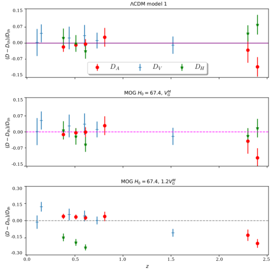
Figure 5: Relative differences between the observable distance ($D_{A}$, $D_{V}$, or $D_{H}$) and the corresponding theoretical prediction for the $\Lambda$CDM model 1 and the MOG models with different values for $H_{0}$ and $V_{G}$. The fiducial $\Lambda$CDM model 1 is shown in the upper panel and $\tilde{\chi}^{2}_{\Lambda{\rm CDM}}=0.94$.

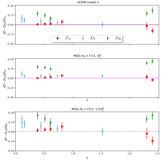
Figure 6: Relative differences between the observable distance ($D_{A}$, $D_{V}$, or $D_{H}$) and the corresponding theoretical prediction for the $\Lambda$CDM model 2 and the MOG models with different values for $H_{0}$ and $V_{G}$. The fiducial $\Lambda$CDM model is shown in the upper panel and $\tilde{\chi}^{2}_{\Lambda{\rm CDM}}=3.68$.

Finally, Table 6 shows that only two MOG models with $H_{0}=67.4$ km sec^-1 Mpc^-1 have theoretical predictions that are in agreement with BAO data within 2$\sigma$ while for the case $H_{0}=73.5$ km sec^-1 Mpc^-1 only one model can explain the data within 5$\sigma$. Besides, all other cases considered in this paper show a reduced $\chi^{2}$ value beyond the customary 5-$\sigma$ equivalent $\tilde{\chi}^{2}_{5\sigma}$. This behavior can also be appreciated in Figs. 5 and 6. Therefore, it should be noted that BAO data, which comprise several independent data sets, as described in Section III.3, provide a useful tool to validate the predictions of the different MOG models analyzed in this paper. On the contrary, the predictions of the MOG models for type Ia supernovae data are very similar to the $\Lambda$CDM fiducial model’s ones, provided $V_{G}\neq 0$. Regarding the cosmic chronometers, even though the predictions for the MOG models do not match the $\Lambda$CDM fiducial model’s one, the large error bars in Fig. 4 prevent this data set to be more conclusive when testing the MOG models.

$V_{G}$	$M$		$\tilde{\chi}^{2}$
	$H_{0}=67.4$	$H_{0}=73.5$	$H_{0}=67.4$	$H_{0}=73.5$
$0$	$-19.20\pm 0.0042$	$-19.01\pm 0.0042$	1.40	1.40
$0.6V_{G}^{M}$	$-19.33\pm 0.0042$	$-19.12\pm 0.0042$	1.08	1.12
$0.8V_{G}^{M}$	$-19.38\pm 0.0042$	$-19.16\pm 0.0042$	1.01	1.05
$0.9V_{G}^{M}$	$-19.40\pm 0.0042$	$-19.18\pm 0.0042$	0.99	1.02
$V_{G}^{M}$	$-19.43\pm 0.0042$	$-19.20\pm 0.0042$	0.98	1.00
$1.1V_{G}^{M}$	$-19.46\pm 0.0042$	$-19.22\pm 0.0042$	0.99	0.98
$1.2V_{G}^{M}$	$-19.49\pm 0.0042$	$-19.25\pm 0.0042$	1.03	0.98

Table 3: Results of the statistical analysis performed with Supernovae type Ia data with fixed nuisance parameters. The table shows the fixed values of $H_{0}$ and $V_{G}$ considered in each case, the obtained best fit value and 1-$\sigma$ error for the absolute magnitude $M$ and the corresponding reduced $\chi^{2}$-value. The equivalent $\chi^{2}$ at 5$\sigma$ is $\tilde{\chi}^{2}_{5\sigma}=1.23$, while for $\Lambda$CDM fiducial models 1 and 2 we obtain $\tilde{\chi}^{2}_{\Lambda{\rm CDM}}=0.98$. $V_{G}^{M}$ is the value suggested in Ref. Moffat and Toth (2007) which also analyses the MOG theory in the cosmological context.

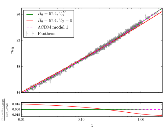
Figure 2: Upper panel: $m_{\rm B}$ for the fiducial $\Lambda$CDM model 1 and MOG models considering $H_{0}=67.4$ km sec^-1 Mpc^-1 and fixed values of $V_{G}$. The data of the Pantheon compilation are shown in gray circles. The $\Lambda$CDM fiducial model 1 and the MOG model with $V_{G}=V_{G}^{M}$ are in agreement with the data within 5$\sigma$ while for the MOG model with $V_{G}=0$ the obtained reduced $\chi^{2}$ value falls beyond the 5-$\sigma$ equivalent. Lower panel: relative differences between the $\Lambda$CDM model 1 and the MOG theory for different values for $H_{0}$ and $V_{G}$.

Figure 3: Upper panel: $m_{\rm B}$ for the fiducial $\Lambda$CDM model 2 and MOG models considering $H_{0}=73.5$ km sec^-1 Mpc^-1 and fixed values of $V_{G}$. The data of the Pantheon compilation are shown in gray circles. The $\Lambda$CDM fiducial model 2 and the MOG model with $V_{G}=V_{G}^{M}$ are in agreement with the data within 5$\sigma$ while for the MOG model with $V_{G}=0$ the obtained reduced $\chi^{2}$ value falls beyond the 5-$\sigma$ equivalent. Lower panel: relative differences between $\Lambda$CDM model 2 and the MOG theory for different values for $H_{0}$ and $V_{G}$.

$H_{0}$	$\alpha$	$\beta$	$\gamma$	$M$	$\tilde{\chi}^{2}$
$67.4$	-	-	-	$-19.43\pm 0.004$	$0.98$
$73.5$	-	-	-	$-19.20\pm 0.004$	$1.00$
$67.4$	$0.158\pm 0.005$	$3.03\pm 0.05$	$0.051\pm 0.009$	$-19.43\pm 0.007$	$0.99$
$73.5$	$0.156\pm 0.005$	$3.00\pm 0.05$	$0.056\pm 0.009$	$-19.19\pm 0.007$	$1.01$
Pantheon	$0.154\pm 0.006$	$3.02\pm 0.06$	$0.053\pm 0.009$

Table 4: Results of the statistical analysis performed with Supernovae type Ia data. In all cases $V_{G}=V_{G}^{M}$. The first column shows the fixed values of $H_{0}$ considered in each case. The first two entries show the results for fixed nuisance parameters given by the Pantheon compilation (also shown in Table 3). The third and fourth entries show the results for the case where the nuisance parameters are allowed to vary. The equivalent $\chi^{2}$ at 5$\sigma$ for the latter is $\tilde{\chi}^{2}_{5\sigma}=1.23$. The last entry shows the values of the nuisance parameters obtained by the Pantheon compilation.

$V_{G}$	$\tilde{\chi}^{2}$
	$H_{0}=67.4$	$H_{0}=73.5$
$0$	7.87	13.64
$0.6V_{G}^{M}$	1.89	5.57
$0.8V_{G}^{M}$	0.78	3.41
$0.9V_{G}^{M}$	0.52	2.49
$V_{G}^{M}$	0.53	1.71
$1.1V_{G}^{M}$	0.94	1.10
$1.2V_{G}^{M}$	1.94	0.71

Table 5: Results of the statistical analysis performed with cosmic chronometers. The table shows the fixed values of $H_{0}$ and $V_{g}$ considered in each case, and the reduced $\chi^{2}$-value. The equivalent $\chi^{2}$ at 5$\sigma$ is $\tilde{\chi}^{2}_{5\sigma}=2.79$ while for the $\Lambda$CDM fiducial models we obtain: $\tilde{\chi}^{2}_{\Lambda{\rm CDM1}}=0.5$ and $\tilde{\chi}^{2}_{\Lambda{\rm CDM2}}=0.74$.

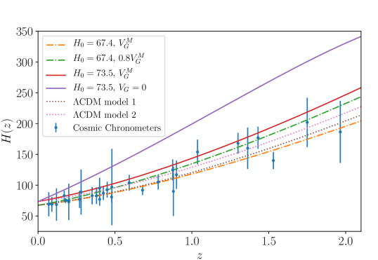
Figure 4: $H(z)$ for the $\Lambda$CDM fiducial models 1 and 2 and the MOG models considering different values for $H_{0}$ and $V_{G}$. The observational data from cosmic chronometers are shown in blue dots. The obtained $\chi^{2}$ values for the MOG model with $H_{0}=73.5$ km sec^-1 Mpc^-1 and $V_{G}=0$ falls beyond the 5-$\sigma$ equivalent while all other models shown in this figure are consistent with the data within 5$\sigma$.

$V_{G}$	$r_{d}/r_{d}^{\rm fid}$		$\tilde{\chi}^{2}$
	$H_{0}=67.4$	$H_{0}=73.5$	$H_{0}=67.4$	$H_{0}=73.5$
$0$	$0.943\pm 0.008$	$0.947\pm 0.008$	46.72	84.82
$0.6V_{G}^{M}$	$0.949\pm 0.008$	$0.924\pm 0.008$	11.72	37.47
$0.8V_{G}^{M}$	$0.967\pm 0.008$	$0.925\pm 0.008$	4.02	23.39
$0.9V_{G}^{M}$	$0.982\pm 0.008$	$0.928\pm 0.008$	1.58	17.08
$V_{G}^{M}$	$1.007\pm 0.008$	$0.934\pm 0.008$	0.9	11.43
$1.1V_{G}^{M}$	$1.047\pm 0.008$	$0.943\pm 0.008$	4.55	6.70
$1.2V_{G}^{M}$	$1.138\pm 0.010$	$0.956\pm 0.008$	28.12	3.39

Table 6: Results of the statistical analysis performed with BAO data. The table shows the fixed values of $H_{0}$ and $V_{G}$ considered in each case, and the corresponding reduced $\chi^{2}$-value. The equivalent $\chi^{2}$ at 5$\sigma$ is $\tilde{\chi}^{2}_{5\sigma}=3.73$ while for the $\Lambda$CDM fiducial models we obtain $\tilde{\chi}^{2}_{\Lambda{\rm CDM1}}=0.94$ and $\tilde{\chi}^{2}_{\Lambda{\rm CDM2}}=3.68$.

V Summary and Conclusions

In this paper we have analyzed the MOG theory in the cosmological context. We considered recent data sets from SNe Ia, BAO and CC to perform $\chi^{2}$ tests. We considered models with fixed values of $H_{0}$ and $V_{G}$, the self-interaction potential of the scalar field that represents the gravitational constant in this theory.

Our results show that none of the predictions of the MOG theory considered here with $V_{G}=0$ is in agreement with the data, which is also consistent with previous results Moffat and Toth (2007, 2013); Jamali and Roshan (2016); Jamali et al. (2018). Regarding the SNe Ia data, we have verified that for different non-zero values of $V_{G}$, the difference between the predictions of the MOG theory is very tiny (in fact, adding more MOG models to Figs 2 and 3 would have been confusing due to the superposition of curves). Conversely, in the case of the CC data, the predictions vary with the value of $V_{G}$ and $H_{0}$, but the large error bars prevent it from being possible to discard more models with this data set. Furthermore, we have also shown that there is agreement between all SNe Ia and all but one CC data and the predictions of the MOG theory. The result is completely different in the case of the statistical analysis with the BAO data set, in which only three models are consistent with the data within 5$\sigma$. Furthermore, it should be stressed that the statistical significance of these latter results is greater when $H_{0}=64.7$ km sec^-1 Mpc^-1 is considered.

On the other hand, the present analysis confirms that the nuisance parameters obtained by the Pantheon compilation assuming the $\Lambda$CDM model are also valid for the MOG theory and therefore it is likely for them to be accurate for other non-standard cosmological models.

In summary, we have analysed the predictions of MOG theory for different values of the Hubble constant and of the self-interaction potential of the scalar field, and compared them to cosmological data of distinct nature, at different redshifts. We have found that most of the studied cases are ruled out by BAO data set, although there are still some values for which the MOG theory cannot be ruled out for any of the data sets considered in this work. This might mean that MOG theory is still a valid alternative to the dark sector of the Universe.

VI Acknowledgements

The authors are supported by the National Agency for the Promotion of Science and Technology (ANPCYT) of Argentina grant PICT-2016-0081; and grants G140 and G157 from UNLP. S.L. acknowledges support from grant UBACYT 20020170100129BA

References

- Oort (1932) J. H. Oort, Bulletin of the Astronomical Institutes of the Netherlands 6, 249 (1932).
- Zwicky (1937) F. Zwicky, Astrophysical Journal 86, 217 (1937).
- Rubin et al. (1978) V. C. Rubin, J. Ford, W. K., and N. Thonnard, Astrophysical Journal l 225, L107 (1978).
- Rubin et al. (1980) V. C. Rubin, J. Ford, W. K., and N. Thonnard, Astrophysical Journal 238, 471 (1980).
- Tyson et al. (1998) J. A. Tyson, G. P. Kochanski, and I. P. Dell’Antonio, Astrophys. J. Lett. 498, L107 (1998), eprint astro-ph/9801193.
- Hasselfield et al. (2013) M. Hasselfield, M. Hilton, T. A. Marriage, G. E. Addison, L. F. Barrientos, N. Battaglia, E. S. Battistelli, J. R. Bond, D. Crichton, S. Das, et al., Journal of Cosmology and Astroparticle Physics 7, 008 (2013), eprint 1301.0816.
- Osato et al. (2018) K. Osato, S. Flender, D. Nagai, M. Shirasaki, and N. Yoshida, Mon. Not. Roy. Astron.Soc. 475, 532 (2018), eprint 1706.08972.
- Planck Collaboration et al. (2016) Planck Collaboration, P. A. R. Ade, N. Aghanim, M. Arnaud, M. Ashdown, J. Aumont, C. Baccigalupi, A. J. Banday, R. B. Barreiro, J. G. Bartlett, et al., Astronomy and Astrophysics 594, A24 (2016), eprint 1502.01597.
- Sakamoto et al. (2003) T. Sakamoto, M. Chiba, and T. C. Beers, Astronomy and Astrophysics 397, 899 (2003), eprint astro-ph/0210508.
- Xue et al. (2008) X. X. Xue, H. W. Rix, G. Zhao, P. Re Fiorentin, T. Naab, M. Steinmetz, F. C. van den Bosch, T. C. Beers, Y. S. Lee, E. F. Bell, et al., Astrophysical Journal 684, 1143 (2008), eprint 0801.1232.
- Kafle et al. (2014) P. R. Kafle, S. Sharma, G. F. Lewis, and J. Bland-Hawthorn, Astrophysical Journal 794, 59 (2014), eprint 1408.1787.
- Iocco et al. (2015) F. Iocco, M. Pato, and G. Bertone, Nature Physics 11, 245 (2015), eprint 1502.03821.
- Scolnic et al. (2018) D. M. Scolnic, D. O. Jones, A. Rest, Y. C. Pan, R. Chornock, R. J. Foley, M. E. Huber, R. Kessler, G. Narayan, A. G. Riess, et al., Astrophysical Journal 859, 101 (2018), eprint 1710.00845.
- Planck Collaboration et al. (2018) Planck Collaboration, N. Aghanim, Y. Akrami, M. Ashdown, J. Aumont, C. Baccigalupi, M. Ballardini, A. J. Banday, R. B. Barreiro, N. Bartolo, et al., arXiv e-prints arXiv:1807.06209 (2018), eprint 1807.06209.
- Ross et al. (2015) A. J. Ross, L. Samushia, C. Howlett, W. J. Percival, A. Burden, and M. Manera, Monthly Notices of the Royal Astronomical Society 449, 835–847 (2015), ISSN 0035-8711, URL http://dx.doi.org/10.1093/mnras/stv154.
- Alam et al. (2017) S. Alam, M. Ata, S. Bailey, F. Beutler, D. Bizyaev, J. A. Blazek, A. S. Bolton, J. R. Brownstein, A. Burden, C.-H. Chuang, et al., Monthly Notices of the Royal Astronomical Society 470, 2617–2652 (2017), ISSN 1365-2966, URL http://dx.doi.org/10.1093/mnras/stx721.
- Abbott et al. (2018) T. M. C. Abbott, F. B. Abdalla, A. Alarcon, S. Allam, F. Andrade-Oliveira, J. Annis, S. Avila, M. Banerji, N. Banik, K. Bechtol, et al., Monthly Notices of the Royal Astronomical Society 483, 4866–4883 (2018), ISSN 1365-2966, URL http://dx.doi.org/10.1093/mnras/sty3351.
- Nuza et al. (2013) S. E. Nuza, A. G. Sánchez, F. Prada, A. Klypin, D. J. Schlegel, S. Gottlöber, A. D. Montero-Dorta, M. Manera, C. K. McBride, A. J. Ross, et al., Mon. Not. Roy. Astron.Soc. 432, 743 (2013), eprint 1202.6057.
- Schumann (2019) M. Schumann, Journal of Physics G Nuclear Physics 46, 103003 (2019), eprint 1903.03026.
- Milgrom (1983) M. Milgrom, Astrophysical Journal 270, 365 (1983).
- Bekenstein (2004) J. D. Bekenstein, Phys. Rev. D 70, 083509 (2004), eprint astro-ph/0403694.
- Clowe et al. (2006a) D. Clowe, M. Bradač, A. H. Gonzalez, M. Markevitch, S. W. Randall, C. Jones, and D. Zaritsky, Astrophysical Journal l 648, L109 (2006a), eprint astro-ph/0608407.
- Moffat (2006) J. W. Moffat, Journal of Cosmology and Gravitation 3, 004 (2006), eprint gr-qc/0506021.
- Moffat and Toth (2008) J. W. Moffat and V. T. Toth, Astrophysical Journal 680, 1158-1161 (2008), eprint 0708.1935.
- Moffat and Rahvar (2014) J. W. Moffat and S. Rahvar, MNRAS 441, 3724 (2014), eprint 1309.5077.
- Moffat and Zhoolideh Haghighi (2017) J. W. Moffat and M. H. Zhoolideh Haghighi, European Physical Journal Plus 132, 417 (2017).
- Moffat and Rahvar (2013) J. W. Moffat and S. Rahvar, MNRAS 436, 1439 (2013), eprint 1306.6383.
- Zhoolideh Haghighi and Rahvar (2017) M. H. Zhoolideh Haghighi and S. Rahvar, MNRAS 468, 4048 (2017), eprint 1609.07851.
- Negrelli et al. (2018) C. Negrelli, M. Benito, S. Landau, F. Iocco, and L. Kraiselburd, Phys. Rev. D 98, 104061 (2018), eprint 1810.07200.
- Clowe et al. (2006b) D. Clowe, M. Bradač, A. H. Gonzalez, M. Markevitch, S. W. Randall, C. Jones, and D. Zaritsky, Astrophysical Journal Letters 648, L109 (2006b), eprint astro-ph/0608407.
- Brownstein and Moffat (2007) J. R. Brownstein and J. W. Moffat, MNRAS 382, 29 (2007), eprint astro-ph/0702146.
- Israel and Moffat (2016) N. S. Israel and J. W. Moffat, ArXiv e-prints (2016), eprint 1606.09128.
- Nieuwenhuizen et al. (2018) T. M. Nieuwenhuizen, A. Morandi, and M. Limousin, Mon. Not. Roy. Astron.Soc. (2018), eprint 1802.04891.
- Boran et al. (2018) S. Boran, S. Desai, E. O. Kahya, and R. P. Woodard, Phys. Rev. D 97, 041501 (2018), eprint 1710.06168.
- Green et al. (2018) M. A. Green, J. W. Moffat, and V. T. Toth, Physics Letters B 780, 300 (2018), eprint 1710.11177.
- Schmidt et al. (1998) B. P. Schmidt, N. B. Suntzeff, M. M. Phillips, R. A. Schommer, A. Clocchiatti, R. P. Kirshner, P. Garnavich, P. Challis, B. Leibundgut, J. Spyromilio, et al., Astrophysical Journal 507, 46 (1998), eprint astro-ph/9805200.
- Tsujikawa (2011) S. Tsujikawa, Dark Energy: Investigation and Modeling, vol. 370 of Astrophysics and Space Science Library (2011).
- De Felice and Tsujikawa (2010) A. De Felice and S. Tsujikawa, Living Reviews in Relativity 13, 3 (2010), eprint 1002.4928.
- Moffat and Toth (2009) J. W. Moffat and V. T. Toth, Classical and Quantum Gravity 26, 085002 (2009), eprint 0712.1796.
- Moffat and Toth (2007) J. W. Moffat and V. T. Toth, arXiv e-prints (2007), eprint 0710.0364.
- Moffat and Toth (2013) J. Moffat and V. Toth, Galaxies 1, 65 (2013).
- Toth (2010) V. T. Toth, arXiv e-prints arXiv:1011.5174 (2010), eprint 1011.5174.
- Jamali and Roshan (2016) S. Jamali and M. Roshan, European Physical Journal C 76, 490 (2016), eprint 1608.06251.
- Jamali et al. (2018) S. Jamali, M. Roshan, and L. Amendola, arXiv e-prints arXiv:1811.04445 (2018), eprint 1811.04445.
- Jimenez and Loeb (2002) R. Jimenez and A. Loeb, Astrophysical Journal 573, 37 (2002), eprint astro-ph/0106145.
- Simon et al. (2005) J. Simon, L. Verde, and R. Jimenez, Phys. Rev. D 71, 123001 (2005), eprint astro-ph/0412269.
- Abraham et al. (2004) R. G. Abraham, K. Glazebrook, P. J. McCarthy, D. Crampton, R. Murowinski, I. Jørgensen, K. Roth, I. M. Hook, S. Savaglio, H.-W. Chen, et al., Astronomical Journal 127, 2455 (2004), eprint astro-ph/0402436.
- Dunlop et al. (1996) J. Dunlop, J. Peacock, H. Spinrad, A. Dey, R. Jimenez, D. Stern, and R. Windhorst, Nature (London) 381, 581 (1996).
- Nolan et al. (2003) L. A. Nolan, J. S. Dunlop, R. Jimenez, and A. F. Heavens, Mon. Not. R. Astron. Soc. 341, 464 (2003), eprint astro-ph/0103450.
- Spinrad et al. (1997) H. Spinrad, A. Dey, D. Stern, J. Dunlop, J. Peacock, R. Jimenez, and R. Windhorst, Astrophysical Journal 484, 581 (1997), eprint astro-ph/9702233.
- Treu et al. (1999) T. Treu, M. Stiavelli, S. Casertano, P. Møller, and G. Bertin, Mon. Not. R. Astron. Soc. 308, 1037 (1999), eprint astro-ph/9904327.
- Treu et al. (2001) T. Treu, M. Stiavelli, P. Møller, S. Casertano, and G. Bertin, Mon. Not. R. Astron. Soc. 326, 221 (2001), eprint astro-ph/0104177.
- Treu et al. (2002) T. Treu, M. Stiavelli, S. Casertano, P. Møller, and G. Bertin, Astrophysical Journal l 564, L13 (2002), eprint astro-ph/0111504.
- Stern et al. (2010a) D. Stern, R. Jimenez, L. Verde, M. Kamionkowski, and S. A. Stanford, JCAP 2, 008 (2010a), eprint 0907.3149.
- Stern et al. (2001) D. Stern, A. Connolly, P. Eisenhardt, R. Elston, B. Holden, P. Rosati, S. A. Stanford, H. Spinrad, P. Tozzi, and K. Wu, in Deep Fields, edited by S. Cristiani, A. Renzini, and R. E. Williams (2001), p. 76, eprint astro-ph/0012146.
- Le Fèvre et al. (2005) O. Le Fèvre, G. Vettolani, B. Garilli, L. Tresse, D. Bottini, V. Le Brun, D. Maccagni, J. P. Picat, R. Scaramella, M. Scodeggio, et al., Astronomy & Astrophysics 439, 845 (2005), eprint astro-ph/0409133.
- Moresco et al. (2012) M. Moresco, A. Cimatti, R. Jimenez, L. Pozzetti, G. Zamorani, M. Bolzonella, J. Dunlop, F. Lamareille, M. Mignoli, H. Pearce, et al., JCAP 8, 006 (2012), eprint 1201.3609.
- Cimatti et al. (2002) A. Cimatti, L. Pozzetti, M. Mignoli, E. Daddi, N. Menci, F. Poli, A. Fontana, A. Renzini, G. Zamorani, T. Broadhurst, et al., Astronomy & Astrophysics 391, L1 (2002), eprint astro-ph/0207191.
- Demarco et al. (2010) R. Demarco, R. Gobat, P. Rosati, C. Lidman, A. Rettura, M. Nonino, A. van der Wel, M. J. Jee, J. P. Blakeslee, H. C. Ford, et al., Astrophysical Journal 725, 1252 (2010), eprint 1009.3986.
- Eisenstein et al. (2001) D. J. Eisenstein, J. Annis, J. E. Gunn, A. S. Szalay, A. J. Connolly, R. C. Nichol, N. A. Bahcall, M. Bernardi, S. Burles, F. J. Castander, et al., Astronomical Journal 122, 2267 (2001), eprint astro-ph/0108153.
- Le Borgne et al. (2006) D. Le Borgne, R. Abraham, K. Daniel, P. J. McCarthy, K. Glazebrook, S. Savaglio, D. Crampton, S. Juneau, R. G. Carlberg, H.-W. Chen, et al., Astrophysical Journal 642, 48 (2006), eprint astro-ph/0503401.
- Lilly et al. (2009) S. J. Lilly, V. Le Brun, C. Maier, V. Mainieri, M. Mignoli, M. Scodeggio, G. Zamorani, M. Carollo, T. Contini, J.-P. Kneib, et al., Astrophysical Journal Supplement Series 184, 218 (2009).
- Onodera et al. (2010) M. Onodera, E. Daddi, R. Gobat, M. Cappellari, N. Arimoto, A. Renzini, Y. Yamada, H. J. McCracken, C. Mancini, P. Capak, et al., Astrophysical Journal l 715, L6 (2010), eprint 1004.2120.
- Rosati et al. (2009) P. Rosati, P. Tozzi, R. Gobat, J. S. Santos, M. Nonino, R. Demarco, C. Lidman, C. R. Mullis, V. Strazzullo, H. Böhringer, et al., Astronomy & Astrophysics 508, 583 (2009), eprint 0910.1716.
- Stern et al. (2010b) D. Stern, R. Jimenez, L. Verde, M. Kamionkowski, and S. A. Stanford, JCAP 2010, 008 (2010b), eprint 0907.3149.
- Strauss et al. (2002) M. A. Strauss, D. H. Weinberg, R. H. Lupton, V. K. Narayanan, J. Annis, M. Bernardi, M. Blanton, S. Burles, A. J. Connolly, J. Dalcanton, et al., Astronomical Journal 124, 1810 (2002), eprint astro-ph/0206225.
- Vanzella et al. (2008) E. Vanzella, S. Cristiani, M. Dickinson, M. Giavalisco, H. Kuntschner, J. Haase, M. Nonino, P. Rosati, C. Cesarsky, H. C. Ferguson, et al., Astronomy & Astrophysics 478, 83 (2008), eprint 0711.0850.
- Zhang et al. (2014) C. Zhang, H. Zhang, S. Yuan, S. Liu, T.-J. Zhang, and Y.-C. Sun, Research in Astronomy and Astrophysics 14, 1221-1233 (2014), eprint 1207.4541.
- Abazajian et al. (2009) K. N. Abazajian, J. K. Adelman-McCarthy, M. A. Agüeros, S. S. Allam, C. Allende Prieto, D. An, K. S. J. Anderson, S. F. Anderson, J. Annis, N. A. Bahcall, et al., Astrophysical Journal Supplement Series 182, 543 (2009), eprint 0812.0649.
- Moresco (2015) M. Moresco, Mon. Not. R. Astron. Soc. 450, L16 (2015), eprint 1503.01116.
- Gobat et al. (2013) R. Gobat, V. Strazzullo, E. Daddi, M. Onodera, M. Carollo, A. Renzini, A. Finoguenov, A. Cimatti, C. Scarlata, and N. Arimoto, Astrophysical Journal 776, 9 (2013), eprint 1305.3576.
- Kriek et al. (2009) M. Kriek, P. G. van Dokkum, I. Labbé, M. Franx, G. D. Illingworth, D. Marchesini, and R. F. Quadri, Astrophysical Journal 700, 221 (2009), eprint 0905.1692.
- Krogager et al. (2014) J. K. Krogager, A. W. Zirm, S. Toft, A. Man, and G. Brammer, Astrophysical Journal 797, 17 (2014), eprint 1309.6316.
- Onodera et al. (2012) M. Onodera, A. Renzini, M. Carollo, M. Cappellari, C. Mancini, V. Strazzullo, E. Daddi, N. Arimoto, R. Gobat, Y. Yamada, et al., Astrophysical Journal 755, 26 (2012), eprint 1206.1540.
- Saracco et al. (2005) P. Saracco, M. Longhetti, P. Severgnini, R. Della Ceca, V. Braito, F. Mannucci, R. Bender, N. Drory, G. Feulner, U. Hopp, et al., Mon. Not. R. Astron. Soc. 357, L40 (2005), eprint astro-ph/0412020.
- Moresco et al. (2016) M. Moresco, L. Pozzetti, A. Cimatti, R. Jimenez, C. Maraston, L. Verde, D. Thomas, A. Citro, R. Tojeiro, and D. Wilkinson, JCAP 5, 014 (2016), eprint 1601.01701.
- Dawson et al. (2013) K. S. Dawson, D. J. Schlegel, C. P. Ahn, S. F. Anderson, É. Aubourg, S. Bailey, R. H. Barkhouser, J. E. Bautista, A. r. Beifiori, A. A. Berlind, et al., Astronomical Journal 145, 10 (2013), eprint 1208.0022.
- Eisenstein et al. (2011) D. J. Eisenstein, D. H. Weinberg, E. Agol, H. Aihara, C. Allende Prieto, S. F. Anderson, J. A. Arns, É. Aubourg, S. Bailey, E. Balbinot, et al., Astronomical Journal 142, 72 (2011), eprint 1101.1529.
- Beutler et al. (2011) F. Beutler, C. Blake, M. Colless, D. H. Jones, L. Staveley-Smith, L. Campbell, Q. Parker, W. Saunders, and F. Watson, Mon. Not. R. Astron. Soc. 416, 3017 (2011), eprint 1106.3366.
- Kazin et al. (2014) E. A. Kazin, J. Koda, C. Blake, N. Padmanabhan, S. Brough, M. Colless, C. Contreras, W. Couch, S. Croom, D. J. Croton, et al., Monthly Notices of the Royal Astronomical Society 441, 3524–3542 (2014), ISSN 0035-8711, URL http://dx.doi.org/10.1093/mnras/stu778.
- Ata et al. (2017) M. Ata, F. Baumgarten, J. Bautista, F. Beutler, D. Bizyaev, M. R. Blanton, J. A. Blazek, A. S. Bolton, J. Brinkmann, J. R. Brownstein, et al., Monthly Notices of the Royal Astronomical Society 473, 4773–4794 (2017), ISSN 1365-2966, URL http://dx.doi.org/10.1093/mnras/stx2630.
- Bautista et al. (2017) J. E. Bautista, N. G. Busca, J. Guy, J. Rich, M. Blomqvist, H. du Mas des Bourboux, M. M. Pieri, A. Font-Ribera, S. Bailey, T. Delubac, et al., Astronomy & Astrophysics 603, A12 (2017), ISSN 1432-0746, URL http://dx.doi.org/10.1051/0004-6361/201730533.
- du Mas des Bourboux et al. (2017) H. du Mas des Bourboux, J.-M. Le Goff, M. Blomqvist, N. G. Busca, J. Guy, J. Rich, C. Yèche, J. E. Bautista, . Burtin, K. S. Dawson, et al., Astronomy & Astrophysics 608, A130 (2017), ISSN 1432-0746, URL http://dx.doi.org/10.1051/0004-6361/201731731.
- Riess et al. (2018) A. G. Riess, S. Casertano, W. Yuan, L. Macri, J. Anderson, J. W. MacKenty, J. B. Bowers, K. I. Clubb, A. V. Filippenko, D. O. Jones, et al., Astrophysical Journal 855, 136 (2018), eprint 1801.01120.