Adversarial Learning Guarantees for
Linear Hypotheses and Neural Networks

Abstract

Adversarial or test time robustness measures the susceptibility of a classifier to perturbations to the test input. While there has been a flurry of recent work on designing defenses against such perturbations, the theory of adversarial robustness is not well understood. In order to make progress on this, we focus on the problem of understanding generalization in adversarial settings, via the lens of Rademacher complexity.

We give upper and lower bounds for the adversarial empirical Rademacher complexity of linear hypotheses with adversarial perturbations measured in $l_{r}$-norm for an arbitrary $r\geq 1$. This generalizes the recent result of Yin et al. (Yin et al., 2019) that studies the case of $r=\infty$, and provides a finer analysis of the dependence on the input dimensionality as compared to the recent work of Khim and Loh (Khim & Loh, 2018) on linear hypothesis classes. We then extend our analysis to provide Rademacher complexity lower and upper bounds for a single ReLU unit. Finally, we give adversarial Rademacher complexity bounds for feed-forward neural networks with one hidden layer. Unlike previous works we directly provide bounds on the adversarial Rademacher complexity of the given network, as opposed to a bound on a surrogate. A by-product of our analysis also leads to tighter bounds for the Rademacher complexity of linear hypotheses, for which we give a detailed analysis and present a comparison with existing bounds.

1 Introduction

Robustness is a key requirement when designing machine learning models and comes in various forms such as robustness to training set corruptions, missing feature values, and model misspecification.In recent years, requiring robustness to adversarial or test time perturbations has become a key requirement. Starting with the work of Szegedy et al. (2014) it has now been well established that deep neural networks trained via standard gradient descent based algorithms are highly susceptible to imperceptible corruptions to the input at test time (Goodfellow et al., 2014; Chen et al., 2017; Eykholt et al., 2018; Carlini & Wagner, 2018). This has led to a proliferation of work aimed at designing classifiers robust to such perturbations (Madry et al., 2017; Gowal et al., 2018, 2019; Schott et al., 2018) and works aimed at designing more sophisticated attacks to break such classifiers (Athalye et al., 2018; Carlini & Wagner, 2017; Sharma & Chen, 2017)

While the above works have made significant progress in designing practical defenses, theoretical aspects of adversarial robustness are currently poorly understood unlike other notions of training set corruptions that have been widely studied in both the statistics and the computer science communities (Huber, 2011; Kearns & Li, 1993; Kearns et al., 1994). Theoretical understanding of adversarial robustness presents three main challenges. The first is a computational one since even checking the robustness of a given model at a given test input is an NP-hard problem (Awasthi et al., 2019). This has been explored in recent works that construct specific instances of learning problems where standard non-robust learning can be done efficiently, but learning a robust classifier becomes computationally hard (Bubeck et al., 2018b, a; Nakkiran, 2019; Degwekar et al., 2019). The second challenge concerns whether achieving adversarial robustness requires one to compromise on standard accuracy. Recent works have shown specific instance where this tradeoff is inherent (Tsipras et al., 2018; Raghunathan et al., 2019).

Finally, the third challenge, the main focus of this work, is the question of what quantity governs generalization in adversarial settings, and how generalization in adversarial settings compares to its non-adversarial counterpart. The recent work of Schmidt et al. (2018) has shown, via specific constructions, that in some scenarios achieving adversarial generalization requires more data as compared to adversarial generalization. Furthermore, the work of Montasser et al. (2019) casts a shadow of doubt on the use of classical quantities such as the VC-dimension of explain generalization in adversarial settings.

However, generalization of function classes of infinite VC dimension (like SVMs with a Gaussian kernel) can be explained via margin based bounds. Characterizing the Rademacher complexity of the function class is essential in these estimates. In a similar vein, we believe that providing non-trivial bounds on the adversarial Rademacher complexity can help shed light on when generalization is possible in adversarial settings via similar margin based bounds. The difficulty is that current bounds on adversarial Rademacher complexity are too loose and vacuous in many settings. This is the barrier that we aim to overcome in this work.

In order to make progress on the mystery of adversarial generalization, a recent line of work (Khim & Loh, 2018; Yin et al., 2019) aims to study the notion of Rademacher complexity for various function classes in the adversarial settings. Focusing mainly on the case of linear models, these works aim to quantify the additional overhead in sample complexity that is incurred when requiring adversarial generalization. Extending the ideas to the case of more general neural networks becomes more challenging and as a result there works instead bound the Rademacher complexity in terms of the Rademacher complexity of an appropriate surrogate. In this work we extend this line of work along several directions.

Our Contributions. We provide a general analysis of the adversarial Rademacher complexity of linear models that holds for perturbations measured in any $\ell_{p}$ norm. This extends the prior work of Yin et al. (2019) that applies only to $\ell_{\infty}$ adversarial perturbation and provided a finer analysis of linear models as compared to the work of Khim & Loh (2018).

As a consequence of our analysis, we provide a sharp characterization of when the adversarial Rademacher complexity suffers from an additional dimension dependent term as compared to its non-adversarial counterpart. This has algorithmic implications for designing appropriate regularizers for adversarial learning of linear models. As an additional byproduct, we are able to provide improved Rademacher complexity bounds for linear classifiers, even in non-adversarial scenarios!

As a next step towards understanding neural networks, we then extend our analysis to provide data dependent upper and lower bounds on the adversarial Rademacher complexity of a single ReLU unit.

Finally, we provide upper bounds on the adversarial Rademacher complexity of one hidden layer neural networks. As opposed to prior works (Yin et al., 2019; Khim & Loh, 2018), our bounds directly apply to the original network as opposed to a surrogate. Our bounds for neural networks come in two forms. We first provide a general upper bound that applies to any neural network with Lipschitz activations. This bound as a dependence on the underlying dimensionality of the input data. Next, we provide a finer data dependent upper bound that is related to the $\epsilon$-adversarial growth function of the data, a quantity we introduce in this work.

Comparison with Prior Work The works of Yin et al. (2019) and Khim and Loh (2018) previously studied the adversarial Rademacher complexity of linear classifiers and neural networks. Our work adds to this line of research in multiple ways. In (Yin et al., 2019) the authors analyze the adversarial Rademacher complexity of linear models when perturbations are measured in $\ell_{\infty}$ norm. They show that in this case the adversarial Rademacher complexity of the loss class is bounded by the sum of its non-adversarial counterpart and a dimension dependent term. Our result is a strict generalization of (Yin et al., 2019) because we provide the analysis of adversarial Rademacher complexity when the perturbations are measured in any general $\ell_{r}$ norm.

The recent work of Khim and Loh (2018) also studies the adversarial Rademacher complexity of linear models under general perturbations. While the bounds are qualitatively similar, our analysis explicitly identifies the dimension dependent term in the general case and as a result can be used to perform better model selection when optimizing the adversarial loss. In addition, we provide a matching lower bound on the adversarial Rademacher complexity of linear models. In the process, we also improve upon the existing classical analysis of (non-adversarial) Rademacher complexity of linear models, which is of independent interest.

For the case of neural networks, both the works of Yin et al. (2019) and Khim and Loh (2018) replace the adversarial loss defined as $\min_{x^{\prime}:\|x^{\prime}-x\|\leq\epsilon}\phi(yf(x^{\prime}))$, by a surrogate upper bound and analyze the resulting Rademacher complexity of the surrogate. In the work of Yin et al. (2019) the surrogate is chosen to be an upper bound on the adversarial loss based on a semi-definite programming (SDP) based relaxation. In the work of (Khim & Loh, 2018) the surrogate is based on the adversarial loss of another neural network that is derived from the original one via a tree based decomposition. In general, these bounds on the surrogate might not lead to meaningful generalization bounds on the original adversarial loss. We instead directly analyze the Rademacher complexity of the adversarial loss.

2 Notation and Preliminaries

We will denote vectors as lowercase bold letters (e.g., ${\mathbf{x}}$) and matrices are uppercase bold (e.g., ${\mathbf{X}}$). The all ones vector is $\mathbf{1}$. Hölder conjugates are denoted by a star (e.g., ${r^{*}}$). For a matrix ${\mathbf{M}}$, the $(p,q)$-group norm is defined as the ${\left|\left|{\mathbf{M}}\right|\right|}_{p,q}=\|(\|{\mathbf{M}}_{1}\|_{1},\ldots,\|{\mathbf{M}}_{d}\|_{p})\|_{q}$, where the ${\mathbf{M}}_{i}$s are the columns of ${\mathbf{M}}$. We focus on binary classification over examples in $\mathbb{R}^{d}$ and adversarial perturbations measured in $\ell_{r}$-norm for $r\geq 1$. Given a loss function $\ell\colon\mathbb{R}\to[0,c]$, we define the loss of a hypothesis $f\colon\mathbb{R}^{d}\to\mathbb{R}$ on a pair $({\mathbf{x}},y)\in\mathbb{R}^{d}\times\{+1,-1\}$ as $\ell_{f}({\mathbf{x}},y)=\ell(yf({\mathbf{x}}))$. As in the standard setting of classification, given a sample $\mathcal{S}=\{({\mathbf{x}}_{1},y_{1}),({\mathbf{x}}_{2},y_{2}),\dots,({\mathbf{x}}_{m},y_{m})\}$ drawn i.i.d. from a distribution $\mathcal{D}$ over $\mathbb{R}^{d}\times\{+1,-1\}$, we define the empirical risk and the expected risk of a hypothesis $f$ as

$$R_{\mathcal{S}}(f) =\frac{1}{m}\sum_{i=1}^{m}\ell_{f}({\mathbf{x}}_{i},y_{i})$$

$$R(f) =\operatorname*{\mathbb{E}}_{\mathcal{S}}[R_{\mathcal{S}}(f)]$$

Given an instance space $\mathcal{Z}$, let $\mathcal{F}$ be a class of functions from $\mathcal{Z}\to\mathbb{R}$. Given $\mathcal{S}=(z_{1},z_{2},\dots,z_{m})\subset\mathcal{Z}^{m}$, the empirical Rademacher complexity of the class $\mathcal{F}$ is defined to be

$$\mathfrak{R}_{\mathcal{S}}(\mathcal{F})=\operatorname*{\mathbb{E}}_{\boldsymbol{\sigma}}\left[\sup_{f\in\mathcal{F}}\frac{1}{m}\sum_{i=1}^{m}\sigma_{i}f(z_{i})\right]$$ (1)

where ${\boldsymbol{\sigma}}$ is a vector of i.i.d. Rademacher random variables. A tight characterization of the uniform convergence of empirical risk to its expected value is given in terms of Rademacher complexity. Good bounds tend to come from margin bounds:

Theorem 1.

(Mohri et al., 2018) Let $\mathcal{F}$ be a family of functions and let $\ell$ be a loss function. Define $\ell_{\mathcal{F}}=\{({\mathbf{x}},y)\mapsto\ell(yf({\mathbf{x}}))\}$. Further, let $\mathcal{S}$ be a sample, and let $\rho>0,\delta>0$. Define $\Phi_{\rho}(x)$ to be the $\rho$-margin loss:

$$\Phi_{\rho}(x)=\min(1,\max(0,1-\frac{x}{\rho}))$$

and set

$$\widehat{R}_{\mathcal{S},\rho}(f)=\frac{1}{m}\sum_{i=1}^{m}\Phi_{\rho}(y_{i}f(x_{i}))$$

Then

$$R(f)\leq\widehat{R}_{\mathcal{S},\rho}(f)+\frac{2}{\rho}\mathfrak{R}_{\mathcal{S}}(\ell_{\mathcal{F}})+3\sqrt{\frac{\log\frac{2}{\delta}}{2m}}$$

holds with probability st least $1-\delta$.

This theorem is significant because margin bounds can yield meaningful guarantees for rich classes even with infinite VC-dimension.

Robust Classification. We now extend the definitions above to their adversarial counterparts. In the setting of adversarially robust classification, the loss at $({\mathbf{x}},y)$ is measured in terms of the worst loss incurred over an adversarial perturbation of ${\mathbf{x}}$ within an $\|\cdot\|_{r}$ ball of a certain radius. We will denote by $\epsilon$ the magnitude of the allowed perturbations. Given $\epsilon>0$, $r\geq 1$, a data point $({\mathbf{x}},y)$, a function $f\colon\mathbb{R}^{d}\to\mathbb{R}$, and a loss function $l\colon\mathbb{R}\to[0,c]$ we define the adversarial loss of $f$ at $({\mathbf{x}},y)$ as

$$\tilde{\ell}_{f}({\mathbf{x}},y)=\sup_{\|{\mathbf{x}}-{\mathbf{x}}^{\prime}\|_{r}\leq\epsilon}\ell(yf({\mathbf{x}}^{\prime}))$$

Similarly, we define the adversarial empirical risk and the adversarial expected risk of a hypothesis $f$ for a sample $\mathcal{S}$ as follows:

$$\widetilde{R}_{\mathcal{S}}(f) =\frac{1}{m}\sum_{i=1}^{m}\tilde{\ell}_{f}({\mathbf{x}}_{i},y_{i})$$

$$\widetilde{R}(f) =\mathbb{E}_{\mathcal{S}}[\widetilde{R}_{\mathcal{S}}(f)]$$

With the above definitions, the following is an immediate application of Theorem 1 above.

Theorem 2 (Robust margin bounds).

Let $\epsilon\geq 0$, $\rho$ and $r\geq 1$. Let $\mathcal{F}$ be a family of functions from $\mathbb{R}^{d}$ to $\mathbb{R}$ and $\ell$ be a loss function taking values in $[0,c]$. For any distribution $\mathcal{D}$ over $\mathbb{R}^{d}\times\{+1,-1\}$, given $\delta>0$, and a sample $\mathcal{S}=(({\mathbf{x}}_{1},y_{1})\cdots({\mathbf{x}}_{m},y_{m}))$ drawn i.i.d. from $\mathcal{D}$, the following holds with probability at least $1-\delta$: $\forall f\in\mathcal{F}$

$$\widetilde{R}(f)\leq\widetilde{R}_{\mathcal{S}}(f)+\frac{2}{\rho}\widetilde{\mathfrak{R}}_{\mathcal{S}}(\ell_{\mathcal{F}})+3c\sqrt{\frac{\log\frac{2}{\delta}}{2m}}.$$ (2)

Here, $\widetilde{\mathfrak{R}}_{\mathcal{S}}(\ell_{\mathcal{F}})$ is the adversarial Rademacher complexity of the class $\ell_{\mathcal{F}}$, and is defined by

$$\widetilde{\mathfrak{R}}_{\mathcal{S}}(\ell_{\mathcal{F}})=\operatorname*{\mathbb{E}}_{\boldsymbol{\sigma}}\left[\sup_{f\in\mathcal{F}}\frac{1}{m}\sum_{i=1}^{m}\sigma_{i}\sup_{\|{{\mathbf{x}}_{i}-{\mathbf{x}}^{\prime}_{i}}\|_{r}\leq\epsilon}\ell(y_{i}f({\mathbf{x}}^{\prime}_{i}))\right].$$ (3)

Throughout the paper, we will assume that the loss function $\ell$ is non-increasing, a property satisfied by many common loss functions including the hinge loss, logistic loss and the exponential loss. In that case, as pointed out in (Yin et al., 2019), the following equality holds:

$$\sup_{\|{{\mathbf{x}}_{i}-{\mathbf{x}}^{\prime}_{i}}\|_{r}\leq\epsilon}\ell(y_{i}f({\mathbf{x}}^{\prime}_{i}))=\ell\Big{(}\inf_{\|{{\mathbf{x}}_{i}-{\mathbf{x}}_{i}^{\prime}}\|_{r}\leq\epsilon}y_{i}f({\mathbf{x}}^{\prime}_{i})\Big{)}.$$

Furthermore, when $\ell(\cdot)$ is $L$-Lipschitz, by Talagrand’s contraction Lemma (Ledoux & Talagrand, 1991), we have $\widetilde{\mathfrak{R}}_{\mathcal{S}}(\ell_{\mathcal{F}})\leq L\mathfrak{R}_{\mathcal{S}}(\widetilde{\mathcal{F}})$, where $\widetilde{\mathcal{F}}$ is the class defined as

$$\widetilde{\mathcal{F}}=\big{\{}({\mathbf{x}},y)\mapsto\inf_{\|{{\mathbf{x}}-{\mathbf{x}}^{\prime}}\|_{r}\leq\epsilon}yf({\mathbf{x}}^{\prime})\colon f\in\mathcal{F}\big{\}}.$$

Hence we get that

$$\widetilde{\mathfrak{R}}_{\mathcal{S}}(\ell_{\mathcal{F}}) \leq L\mathfrak{R}_{\mathcal{S}}(\widetilde{\mathcal{F}})$$

$$=L\operatorname*{\mathbb{E}}_{\boldsymbol{\sigma}}\left[\sup_{f\in\mathcal{F}}\frac{1}{m}\sum_{i=1}^{m}\sigma_{i}\inf_{\|{{\mathbf{x}}_{i}-{\mathbf{x}}^{\prime}_{i}}\|_{r}\leq\epsilon}y_{i}f({\mathbf{x}}^{\prime}_{i})\right].$$ (4)

Providing sharp bounds for (4) for various function classes $\mathcal{F}$ will be the central focus of this work.

3 Adversarial Rademacher Complexity of Linear Hypotheses

In this section we provide a sharp characterization of the adversarial Rademacher complexity, as defined in (4), for linear function classes with bounded $p$-norm and with perturbations measured in any $r$-norm. Prior work (Yin et al., 2019) studied the case when the perturbations are measured in the $\ell_{\infty}$-norm. Our general analysis leads to a deeper understanding of the interplay between the complexity of the hypothesis classes (measured in $p$-norm) and the perturbation set (measured in $r$-norm), and how this dictates whether one can expect an additional dimension dependent penalty in the adversarial case over its non-adversarial counterpart. Furthermore, our analysis explicitly characterizes the dimension dependent term on which the adversarial Rademacher complexity depends on. This provides a finer analysis than the work of Khim & Loh (2018) and also has algorithmic implications. Formally, we study the case when

$$\mathcal{F}_{p}=\{{\mathbf{x}}\mapsto\left\langle{\mathbf{w}},{\mathbf{x}}\right\rangle\colon\|{{\mathbf{w}}}\|_{p}\leq W\}$$ (5)

3.1 Rademacher Complexity of Linear Hypotheses

A crucial aspect of our analysis in the linear case is a more general upper bound on the Rademacher complexity of $p$-norm bounded linear function classes, in the non-adversarial case. We first state this general bound as it will play an important role in later sections when analyzing the adversarial Rademacher complexity of ReLU functions and more general neural networks.

Theorem 3.

Let $\mathcal{F}_{p}$ be the class of functions defined in (5). Then, given a sample $\mathcal{S}=\{({\mathbf{x}}_{1},y_{1}),\dots,({\mathbf{x}}_{m},y_{m})\}$ we have

$$\mathfrak{R}_{\mathcal{S}}(\mathcal{F}_{p})\leq\begin{cases}\frac{W}{m}\sqrt{{2\log(2d)}}\|{{\mathbf{X}}^{T}}\|_{2,\infty}&\text{if $p=1$}\\ \frac{\sqrt{2}W}{m}\bigg{[}\frac{\Gamma(\tfrac{{p^{*}}+1}{2})}{\sqrt{\pi}}\bigg{]}^{\frac{1}{{p^{*}}}}\|{{\mathbf{X}}^{T}}\|_{2,{p^{*}}}&\text{if $1<p\leq 2$}\\ \frac{W}{m}\|{\mathbf{X}}^{T}\|_{2,{p^{*}}}&\text{if $p\geq 2$}\end{cases}$$

Here ${\mathbf{X}}$ is the $d\times m$ matrix with the data points ${\mathbf{x}}_{i}$ as columns. We make a few remarks about the theorem above and defer its proof to Appendix A.2. Some well-known bounds on the Rademacher complexity of $\mathcal{F}_{p}$ are

$$\mathfrak{R}_{\mathcal{S}}(\mathcal{F}_{p})\leq\begin{cases}W\sqrt{\frac{2\log(2d)}{m}}\|{\mathbf{X}}\|_{\max}&\text{ if $p=1$}\\ \frac{W}{m}\sqrt{{p^{*}}-1}\|{{\mathbf{X}}}\|_{{p^{*}},2}&\text{ if $1<p\leq 2$}\end{cases}$$ (6)

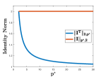
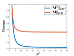
(a)	(b)

Figure 1: (a) A plot comparing two norms of the $4\times 4$ identity matrix, $\|{\mathbf{I}}^{T}\|_{2,{p^{*}}}$ and $\|{\mathbf{I}}\|_{{p^{*}},2}$; the lower bound on the ratio of the two norms (7) in Proposition 1 holds for this matrix. (b) Same as (a), but for Gaussian matrices.

Although the case $p\in[1,2]$ in the theorem above is known (Kakade et al., 2008; Mohri et al., 2018), we provide a simpler proof of in Appendix A.1. The inequality for $p=1$ is further reproduced for completeness. Our new bound coincides with (6) when $p=2$ and is strictly better otherwise. Readers familiar with Rademacher complexity bounds for linear functions will notice that our bound in this case depends on the norm $\|{\mathbf{X}}^{T}\|_{2,p^{*}}$. In contrast, standard bounds on the Rademacher complexity of linear classes depend on $\|{\mathbf{X}}\|_{p^{*},2}$. In fact one can show that the $\|{\mathbf{X}}^{T}\|_{2,p^{*}}$ is always smaller than $\|{\mathbf{X}}\|_{p^{*},2}$ for $p\in(1,2]$, that is $p^{*}\geq 2$, as shown by the last inequality of (7) in the following proposition.

Proposition 1.

Let ${\mathbf{M}}$ be a $d\times m$ matrix. If $q\leq p$, then

$$\min(m,d)^{\frac{1}{p}-\frac{1}{q}}\|{\mathbf{M}}^{T}\|_{p,q}\leq\|{\mathbf{M}}\|_{q,p}\leq\|{\mathbf{M}}^{T}\|_{p,q}$$ (7)

If $q\geq p$, then

$$\min(m,d)^{\frac{1}{p}-\frac{1}{q}}\|{\mathbf{M}}^{T}\|_{p,q}\geq\|{\mathbf{M}}\|_{q,p}\geq\|{\mathbf{M}}^{T}\|_{p,q}$$ (8)

These bounds are tight.

The proof is deferred to Appendix A.4. To visualize the ratio between these two norms, we plot the two norms for various values of ${p^{*}}$ in Figure 1. For convenience, in the discussion below, we set $c_{1}(p)=\sqrt{{p^{*}}-1}$ and $c_{2}(p)=\sqrt{2}\big{[}\frac{\Gamma(\tfrac{{p^{*}}+1}{2})}{\sqrt{\pi}}\big{]}^{\frac{1}{{p^{*}}}}$. Regarding the growth of the constant in our bound, one can show that as ${p^{*}}\to\infty$, $c_{2}(p)$ grows asymptotically like $e^{-\frac{1}{2}}\sqrt{{p^{*}}}$. In fact one can show that

$$e^{-\frac{1}{2}}\sqrt{{p^{*}}}\leq c_{2}(p)\leq e^{-\frac{1}{2}}\sqrt{{p^{*}}+1}$$

Furthermore, $c_{2}(p)\leq c_{1}(p)$ in the relevant region (see Appendix A.5). In Figure 2 we plot $c_{1}(p),c_{2}(p)$ and the bounds on $c_{1}(p)$ and $c_{2}(p)$ to illustrate the growth rate of these constants with ${p^{*}}$.

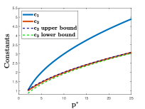
Figure 2: A plot of $c_{1}(p)$, $c_{2}(p)$, and the bounds from Lemma 4. Note that $c_{1}(2)=c_{2}(2)$ and that the upper and lower bounds on $c_{2}$ are tight.

Proposition 1 and that $c_{2}(p)\leq c_{1}(p)$ imply that the bounds we give for linear classes are stronger than what was previously known.

3.2 Adversarial Rademacher Complexity of Linear Hypotheses

We now extend our bounds from the previous section to provide a complete characterization of the adversarial Rademacher complexity of linear function classes under arbitrary $r$-norm perturbations. These theorems improve upon the recent work of Yin et al. (2019) that studies $\infty$-norm perturbations and provide a finer analysis, with a matching lower bound, as compared to the recent work of Khim & Loh (2018). Our main result is stated below.

Theorem 4.

Let $\epsilon>0$, $p,r\geq 1$. Consider a sample $\mathcal{S}=\{({\mathbf{x}}_{1},y_{1}),\dots,({\mathbf{x}}_{m},y_{m})\}$ with ${\mathbf{x}}_{i}\in\mathbb{R}^{d}$ and $y_{i}\in\{\pm 1\}$. Let $\mathcal{F}_{p}$ be the class of linear functions defined in (5). Then it holds that

$$\widetilde{\mathfrak{R}}_{\mathcal{S}}(\mathcal{F}_{p}) \leq\bigg{(}\mathfrak{R}_{\mathcal{S}}(\mathcal{\mathcal{F}}_{p})+\epsilon\frac{W}{2\sqrt{m}}\max(d^{1-\frac{1}{r}-\frac{1}{p}},1)\bigg{)}$$

and

$$\widetilde{\mathfrak{R}}_{\mathcal{S}}(\mathcal{F}_{p}) \geq\max\bigg{(}\mathfrak{R}_{\mathcal{S}}(\mathcal{F}_{p}),{W}\frac{\epsilon\max(d^{1-\frac{1}{r}-\frac{1}{p}},1)}{2\sqrt{2m}}\bigg{)}.$$

Notice that when the perturbation is measured in $\ell_{\infty}$-norm, i.e. $r=\infty$, we recover the bound of Yin et al. (2019). Hence the theorem above is a strict generalization of the result of Yin et al. (2019). Furthermore, when $\epsilon=0$, as expected, the adversarial Rademacher complexity equals the standard Rademacher complexity of linear models and we can use our improved bounds from Theorem 3. The theorem above has important implications for the design of regularizers in the context of adversarial learning of linear models. As suggested by the upper bounds above, if $1/r+1/p\geq 1$, then one can indeed perform adversarially robust learning with minimal statistical overhead in the standard classification setting! More specifically, in this case the upper bound on the adversarial Rademacher complexity has at most $W\epsilon/\sqrt{m}$ overhead on top of the standard bound from Theorem 3 and is dimension independent. Noting that $1-1/r=1/r^{*}$, we get that for statistical efficiency one should choose a $p$-norm regularizer on ${\mathbf{w}}$, where $p\in[1,r^{*}]$. Our lower bound on the other hand shows that any other choice of a $\ell_{p}$-norm based regularizer will necessarily incur a dimension-dependent penalty.

3.3 Proof sketch of Theorem 4

We provide a brief sketch of the proof of Theorem 4 and provide the details in Appendix B. As a first step, a simple argument shows that

$$\inf_{\|{\mathbf{x}}-{\mathbf{x}}^{\prime}\|_{r}\leq\epsilon}y({\mathbf{w}}\cdot{\mathbf{x}}^{\prime})=y{\mathbf{w}}\cdot{\mathbf{x}}-\epsilon\|{\mathbf{w}}\|_{r^{*}}.$$

Using the above, we can write the adversarial Rademacher complexity as:

$$\mathfrak{R}_{\mathcal{S}}(\widetilde{\mathcal{F}}_{p})=\operatorname*{\mathbb{E}}_{\boldsymbol{\sigma}}{\left[\sup_{\|{\mathbf{w}}\|_{p}\leq W}\left\langle{\mathbf{w}},{\mathbf{u}}_{\boldsymbol{\sigma}}\right\rangle-\epsilon v_{\boldsymbol{\sigma}}\|{\mathbf{w}}\|_{{r^{*}}}\right]}$$ (9)

where, for convenience, we set ${\mathbf{u}}_{\boldsymbol{\sigma}}=\frac{1}{m}\sum_{i=1}^{m}y_{i}\sigma_{i}{\mathbf{x}}_{i}$, $v_{\boldsymbol{\sigma}}=\frac{1}{m}\sum_{i=1}^{m}\sigma_{i}$. Next, we present two key lemmas.

Lemma 1.

Let $1\leq p,r\leq\infty$ and let $d$ be the dimension. Then

$$\sup_{\|{\mathbf{w}}\|_{p}\leq 1}\|{\mathbf{w}}\|_{{r^{*}}}=\max(1,d^{1-\frac{1}{r}-\frac{1}{p}})$$

Lemma 2.

Let $v_{\boldsymbol{\sigma}}=\frac{1}{m}\sum_{i=1}^{m}\sigma_{i}$. Then it holds that

$$\operatorname*{\mathbb{E}}_{\boldsymbol{\sigma}}\left[{\sup_{\|{\mathbf{w}}\|_{p}\leq W}v_{\boldsymbol{\sigma}}\|{\mathbf{w}}\|_{{r^{*}}}}\right]\geq\frac{W\epsilon\max(d^{1-\frac{1}{r}-\frac{1}{p}},1)}{{2\sqrt{2m}}},$$

and

$$\operatorname*{\mathbb{E}}_{\boldsymbol{\sigma}}\left[{\sup_{\|{\mathbf{w}}\|_{p}\leq W}v_{\boldsymbol{\sigma}}\|{\mathbf{w}}\|_{{r^{*}}}}\right]\leq\frac{W\epsilon\max(d^{1-\frac{1}{r}-\frac{1}{p}},1)}{2\sqrt{m}}$$

For the upper bound, using the sub-additivity of supremum and Lemma 2 yields

$$\mathfrak{R}_{\mathcal{S}}(\widetilde{\mathcal{F}}_{p}) \leq\mathfrak{R}_{\mathcal{S}}(\mathcal{F}_{p})+\epsilon\operatorname*{\mathbb{E}}_{{\boldsymbol{\sigma}}}\left[\sup_{\|{\mathbf{w}}\|_{p}\leq W}v_{\boldsymbol{\sigma}}\|{\mathbf{w}}\|_{{r^{*}}}\right]$$

$$=\mathfrak{R}_{\mathcal{S}}(\mathcal{F}_{p})+\frac{1}{2}\epsilon\frac{W}{\sqrt{m}}\max(d^{1-\frac{1}{r}-\frac{1}{p}},1).$$

For the lower bound, we apply two symmetrization arguments and show that

$$\mathfrak{R}_{\mathcal{S}}(\widetilde{\mathcal{F}}_{p}) =\operatorname*{\mathbb{E}}_{{\boldsymbol{\sigma}}}\left[\sup_{\|{\mathbf{w}}\|_{p}\leq W}-\left\langle{\mathbf{w}},{\mathbf{u}}_{\sigma}\right\rangle+\epsilon v_{\boldsymbol{\sigma}}\|{\mathbf{w}}\|_{{r^{*}}}\right]$$ (10)

$$=\operatorname*{\mathbb{E}}_{{\boldsymbol{\sigma}}}\left[\sup_{\|{\mathbf{w}}\|_{p}\leq W}\left\langle{\mathbf{w}},{\mathbf{u}}_{\boldsymbol{\sigma}}\right\rangle+\epsilon v_{\boldsymbol{\sigma}}\|{\mathbf{w}}\|_{{r^{*}}}\right].$$ (11)

Averaging equations (9) and (11) and applying the sub-additivity of supremum gives:

$$\mathfrak{R}_{\mathcal{S}}(\widetilde{\mathcal{F}}_{p}) =\frac{1}{2}\operatorname*{\mathbb{E}}_{{\boldsymbol{\sigma}}}\left[\sup_{\|{\mathbf{w}}\|_{p}\leq W}\left\langle{\mathbf{w}},{\mathbf{u}}_{\boldsymbol{\sigma}}\right\rangle-\epsilon v_{\boldsymbol{\sigma}}\|{\mathbf{w}}\|_{{r^{*}}}\right]$$

$$\quad+\frac{1}{2}\operatorname*{\mathbb{E}}_{{\boldsymbol{\sigma}}}\left[\sup_{\|{\mathbf{w}}\|_{p}\leq W}\left\langle{\mathbf{w}},{\mathbf{u}}_{\boldsymbol{\sigma}}\right\rangle+\epsilon v_{\boldsymbol{\sigma}}\|{\mathbf{w}}\|_{{r^{*}}}\right]$$

$$\geq\operatorname*{\mathbb{E}}_{{\boldsymbol{\sigma}}}\left[\sup_{\|{\mathbf{w}}\|_{p}\leq W}\left\langle{\mathbf{w}},{\mathbf{u}}_{\boldsymbol{\sigma}}\right\rangle\right]=W\mathfrak{R}_{\mathcal{S}}({\mathcal{F}_{p}}).$$

Now averaging (10) and (11), applying sub-additivity and Lemma 2, the following holds:

$$\mathfrak{R}_{\mathcal{S}}(\widetilde{\mathcal{F}}_{p}) =\frac{1}{2}\operatorname*{\mathbb{E}}_{{\boldsymbol{\sigma}}}\left[\sup_{\|{\mathbf{w}}\|_{p}\leq W}-\left\langle{\mathbf{w}},{\mathbf{u}}_{\boldsymbol{\sigma}}\right\rangle+\epsilon v_{\boldsymbol{\sigma}}\|{\mathbf{w}}\|_{{r^{*}}}\right]$$

$$\quad+\frac{1}{2}\operatorname*{\mathbb{E}}_{{\boldsymbol{\sigma}}}\left[\sup_{\|{\mathbf{w}}\|_{p}\leq W}\left\langle{\mathbf{w}},{\mathbf{u}}_{\boldsymbol{\sigma}}\right\rangle+\epsilon v_{\boldsymbol{\sigma}}\|{\mathbf{w}}\|_{{r^{*}}}\right]$$

$$\geq\operatorname*{\mathbb{E}}_{{\boldsymbol{\sigma}}}\left[\sup_{\|{\mathbf{w}}\|_{p}\leq W}v_{\boldsymbol{\sigma}}\|{\mathbf{w}}\|_{r^{*}}\right]$$

$$\geq\frac{W}{2\sqrt{2m}}\epsilon\max(d^{1-\frac{1}{p}-\frac{1}{r}},1).$$

4 Adversarial Rademacher Complexity of a Rectified Linear Unit

As a first step towards providing a bound for neural networks, in this section we study the adversarial Rademacher complexity of linear functions composed with a rectified linear unit (ReLU). Again we measure the size of functions in $p$ norm and define the function class by

$$\mspace{-8.0mu}\mathcal{G}_{p}=\{({\mathbf{x}},y)\mapsto(y\left\langle{\mathbf{w}},{\mathbf{x}}\right\rangle)_{+}\colon\|{\mathbf{w}}\|_{p}\leq W,y\in\{-1,1\}\}$$ (12)

where $(z)_{+}=\max(z,0)$. The following theorem presents a data-dependent upper bound on the adversarial Rademacher complexity of the ReLU unit.

Theorem 5.

Let $\mathcal{G}_{p}$ be the class as defined in (12) and let $\mathcal{F}_{p}$ be the corresponding linear class as defined in (5). Then, given a sample $\mathcal{S}=\{({\mathbf{x}}_{1},y_{1}),\dots,({\mathbf{x}}_{m},y_{m})\}$, the adversarial Rademacher complexity of $\mathcal{G}_{p}$ can be bounded as follows:

$$\widetilde{\mathfrak{R}}_{\mathcal{S}}(\mathcal{G}_{p}) \leq{\mathfrak{R}}_{T_{\epsilon}}(\mathcal{F}_{p})+\epsilon\frac{W}{2\sqrt{m}}\max(1,d^{1-\frac{1}{r}-\frac{1}{p}}),$$

where $T_{\epsilon}=\{i\colon y_{i}=-1\text{ or },y_{i}=1\text{ and }\|{{\mathbf{x}}_{i}}\|_{r}>\epsilon\}$.

The second term in the bound above is similar to the dimension dependent term that appears in the linear case. The first term is the empirical Rademacher complexity of linear classes with bounded $p$-norm, but only measured on a carefully chosen subset of the data. This implies that data points with positive labels that have small norm as compared to the perturbation $\epsilon$ do not affect the Rademacher complexity. Hence, the guarantee in the theorem treats the two classes $+1$ and $-1$ asymmetrically.

This phenomenon originates from a property of the function $(z)_{+}$. Recall that in our setup $(z)_{+}$ will later be composed with a loss function $\ell$. Because $\ell(yz_{+})$ is the penalty incurred to the loss, the value $yz_{+}$ should be interpreted as a margin. Since the function $\max(0,z)$ is always 0 for $z\leq 0$, decreasing $z$ below 0 does not affect the the margin. On the other hand increasing $z$ above zero will increase the margin. A large margin for a point labeled $-1$ corresponds to making $z_{+}$ as small as possible. As a result, every $z$ with $z\leq 0$ gives the same margin. However, there is no upper bound on the margin for points in the class $+1$. As a result, the classifier $(y,{\mathbf{x}})\mapsto y(\left\langle{\mathbf{w}},{\mathbf{x}}\right\rangle)_{+}$ treats all non-negative margins for the class $-1$ in the same manner, but gives a higher reward for larger margins for the class $+1$.

This observation has implications for adversarial classification; as shown in Appendix C, an adversarially perturbed ReLU is $y\max({\mathbf{w}}\cdot{\mathbf{x}}-\epsilon y\|{\mathbf{w}}\|_{r^{*}},0)$. If ${\mathbf{w}}\cdot{\mathbf{x}}$ is very negative, which corresponds to high confidence for $y=-1$, then the perturbation would not change the value of the loss function. On the other hand, if ${\mathbf{w}}\cdot{\mathbf{x}}$ were large and positive, a perturbation would definitely change the value of the margin and then influence the loss. We next complement our upper bound with a data dependent lower bound, stated below, on the adversarial Rademacher complexity.

Theorem 6.

Let $\mathcal{G}_{p}$ be the class as defined in (12). Then it holds that

$$\widetilde{\mathfrak{R}}_{\mathcal{S}}(\mathcal{G}_{p})\geq\frac{W}{2\sqrt{2}m}\sup_{\|{\mathbf{s}}\|_{p}=1}\bigg{(}\sum_{i\in T_{\epsilon,{\mathbf{s}}}}(\left\langle{\mathbf{s}},{\mathbf{x}}_{i}\right\rangle-\epsilon y_{i}\|{\mathbf{s}}\|_{r^{*}})^{2}\bigg{)}^{\frac{1}{2}}$$

where $T_{\epsilon,{\mathbf{s}}}=\{i\colon\left\langle{\mathbf{s}},{\mathbf{x}}_{i}\right\rangle-y_{i}\epsilon\|{\mathbf{s}}\|_{r^{*}}>0\}$.

A natural question that comes to mind is if one can characterize scenarios where the above lower bound leads to a dimension dependent term, as in the lower bound for linear hypotheses. In order to characterize this, for a given $s$ and $\delta>0$, define the set $T^{\delta}_{\epsilon,{\mathbf{s}}}$ as

$$T^{\delta}_{\epsilon,{\mathbf{s}}}=\{i\colon\left\langle{\mathbf{s}},{\mathbf{x}}_{i}\right\rangle-(1+\delta y_{i})y_{i}\epsilon\|{\mathbf{s}}\|_{r^{*}}>0\}.$$

Notice that $T^{\delta}_{\epsilon,{\mathbf{s}}}$ is a subset of $T_{\epsilon,{\mathbf{s}}}$ and contains points in $T^{\delta}_{\epsilon,{\mathbf{s}}}$ that have a non-trivial margin. Then we get that

$$\mathfrak{R}_{\mathcal{S}}(\mathcal{G}_{p}) \geq\frac{W}{2\sqrt{2}m}\sup_{\|{\mathbf{s}}\|_{p}=1}\bigg{(}\sum_{i\in T^{\delta}_{\epsilon,{\mathbf{s}}}}(\left\langle{\mathbf{s}},{\mathbf{x}}_{i}\right\rangle-\epsilon y_{i}\|{\mathbf{s}}\|_{r^{*}})^{2}\bigg{)}^{\frac{1}{2}}$$

$$\geq\frac{W}{2\sqrt{2}m}\sup_{\|{\mathbf{s}}\|_{p}=1}\bigg{(}\sum_{i\in T^{\delta}_{\epsilon,{\mathbf{s}}}}(\delta\epsilon\|{\mathbf{s}}\|_{r^{*}})^{2}\bigg{)}^{\frac{1}{2}}$$

$$=\frac{W\delta\epsilon}{2\sqrt{2}m}\sup_{\|{\mathbf{s}}\|_{p}=1}|T^{\delta}_{\epsilon,{\mathbf{s}}}|\|{\mathbf{s}}\|_{{r^{*}}}.$$

Denoting ${\mathbf{s}}^{*}$ to be the vector that achieves the value $\sup_{\|{\mathbf{s}}\|_{p}=1}\|{\mathbf{s}}\|_{{r^{*}}}$ we get that

$$\mathfrak{R}_{\mathcal{S}}(\mathcal{G}_{p}) \geq\frac{W\delta\epsilon}{2\sqrt{2}m}|T^{\delta}_{\epsilon,{\mathbf{s}}^{*}}|\max(d^{1-\frac{1}{p}-\frac{1}{r}},1).$$

Hence, if for a given constant $\delta>0$, the size of the set $T^{\delta}_{\epsilon,{\mathbf{s}}^{*}}$ is large then we expect a dimension dependent lower bound similar to the linear case.

5 Adversarial Rademacher Complexity of Neural Nets

Building on our analysis for the case of a single ReLU unit, we next give an upper bound on the adversarial Rademacher complexity for the class of one-layer neural networks comprised of a Lipschitz activation $\rho$ with $\rho(0)=0$. The guarantees of our theorem resemble the bound on the standard Rademacher complexity of neural networks, as provided in (Cortes et al., 2017). An analysis based on other forms of generalization bounds on neural nets is also possible, such as that of Bartlett et al. (2017). The family of functions of such one-layer neural networks is defined as follows:

$$\mathcal{G}^{n}_{p}=\Big{\{}({\mathbf{x}},y)\mapsto y\sum_{j=1}^{n}u_{j}\rho({\mathbf{w}}_{j}\cdot{\mathbf{x}})\colon\|{\mathbf{u}}\|_{1}\leq\Lambda,\|{{\mathbf{w}}_{j}}\|_{p}\leq W\Big{\}}.$$

Our main theorem is stated below.

Theorem 7.

Let $\rho$ be a function with Lipschitz constant $L_{\rho}$ with $\rho(0)=0$ and consider perturbations in $r$-norm. Then, the following upper bound holds for the adversarial Rademacher complexity of $\mathcal{G}^{n}_{p}$:

$$\widetilde{\mathfrak{R}}_{\mathcal{S}}(\mathcal{G}_{p}^{n}) \leq L_{\rho}\bigg{[}\frac{W\Lambda\max(1,d^{1-\frac{1}{p}-\frac{1}{r}})(\|{\mathbf{X}}\|_{r,\infty}+\epsilon)}{\sqrt{m}}\bigg{]}\times$$

$$\quad\left(1+\sqrt{d(n+1)\log(36)}\right).$$

The proof is presented in Appendix D. The only requirements on our activation function $\rho$ is that it is Lipschitz and $\rho(0)=0$. This stipulation is satisfied by common activation functions like the ReLU, the leaky ReLU, and the hyperbolic tangent, but not the sigmoid or a step function. In comparison to the adversarial Rademacher complexity of linear classifiers, Theorem 7 still includes a $\max(1,d^{1-\frac{1}{r}-\frac{1}{p}})$ factor, again implying that one should choose a model class with $p\leq{r^{*}}$. The complexity of the vector ${\mathbf{u}}$ is bounded by $\ell_{1}$ norm as that is what turns out to be natural in the proof. However, the dimension dependence is larger by a factor of $\sqrt{d}$. The dependence on the number of neurons $(\sqrt{n})$ is also problematic. This fact is unfortunate since a much larger sample size $m$ would be required for good generalization. In the next section we present a promising approach towards removing the dependence on dimension and the number of neurons in the above bound.

6 Towards Dimension-Independent Bounds

In this section we introduce a new framework for analyzing the adversarial Rademacher complexity of neural networks with ReLU activations. Unlike the case of linear hypotheses, the dimension-dependent term in the upper bound in Theorem 7 cannot be avoided by simply picking the appropriate norm $p$. In particular, deriving dimension-independent bounds for the adversarial Rademacher complexity of neural networks is a difficult problem. Prior works (Yin et al., 2019; Khim & Loh, 2018) have resorted to bounding the adversarial Rademacher complexity of surrogates that are more tractable. However, it is not clear how those guarantees translate into meaningful bounds on the complexity of the original network. In this section, we present an approach towards obtaining dimension-independent bounds on the adversarial Rademacher complexity of the original network.

A major component of the difficultly in analyzing adversarial Rademacher complexity relates to providing a tight characterization of the optimal adversarial perturbation for a given point ${\mathbf{x}}_{i}$, i.e.,

$${\mathbf{s}}^{*}_{i}=\operatorname*{argmin}_{{\mathbf{s}}:\|{\mathbf{s}}\|_{r}\leq 1}y_{i}\sum_{j=1}^{n}u_{j}({\mathbf{w}}_{j}\cdot({\mathbf{x}}_{i}+\epsilon{\mathbf{s}}))_{\plus}$$ (13)

Thus, to begin, we study properties of such adversarial perturbations to the neural network. Afterwards, we leverage these properties to bound the adversarial Rademacher complexity. Notably, the proofs of these properties heavily rely on the fact that the activation function is ReLU and not any other Lipschitz function. As in the previous section, we will focus on the family of a one layer-network $\mathcal{G}^{n}_{p}$ with activation $\rho(z)=z_{+}$.

6.1 Characterizing Adversarial Perturbations

In this section, we discuss characteristics of adversarial perturbations to neural networks with ReLU activations. The following theorem implies that, if the perturbations are bounded in $\ell_{r}$-norm by $\epsilon$, then typically the optimal adversarial perturbations will have exactly $r$-norm $\epsilon$.

Theorem 8.

Let $d$ be the dimension and $n$ the number of neurons. Consider the problem

$$\inf_{\|{\mathbf{s}}\|_{r}\leq 1}f({\mathbf{s}})=\sum_{j=1}^{n}u_{j}({\mathbf{w}}_{j}\cdot({\mathbf{x}}+\epsilon{\mathbf{s}}))_{+}.$$ (14)

If either $\|{\mathbf{x}}\|_{r}\geq\epsilon$ or $n<d$, an optimum is attained on the sphere $\{{\mathbf{s}}\colon\|{\mathbf{s}}\|_{r}=1\}$. Otherwise, an optimum is attained either at ${\mathbf{s}}=-\frac{1}{\epsilon}{\mathbf{x}}$ or on $\|{\mathbf{s}}\|_{r}=1$.

The proof of the above theorem is deferred to Appendix E.1. Theorem 8 implies that if $n<d$, then the optimal perturbation always has norm $\epsilon$. This result is significant because $n<d$ is a common scenario. At the same time, the theorem also implies that if $\|{\mathbf{x}}\|_{r}\geq\epsilon$, then the optimal perturbation still has norm $\epsilon$. In practice, one expects the norm of the data points to be larger than the perturbation. Thus, on real world datasets, one would expect adversarial perturbations to always have norm $\epsilon$.

For $1<r<\infty$, Theorem 8 aids in finding a necessary condition for the optimum. This condition implies that critical points are characterized by specifying which ${\mathbf{w}}_{j}$ satisfy ${\mathbf{w}}_{j}\cdot({\mathbf{x}}+\epsilon{\mathbf{s}})<0,{\mathbf{w}}_{j}\cdot({\mathbf{x}}+\epsilon{\mathbf{s}})=0$, and ${\mathbf{w}}_{j}\cdot({\mathbf{x}}+\epsilon{\mathbf{s}})>0$. The exact assertion is fairly involved, so we delay the statement of this theorem to Appendix E.2. However, the theorem simplifies considerably for $r=2$ and we include this case below.

Theorem 9.

Assume that $\|{\mathbf{x}}\|_{r}\geq\epsilon$. Let $1<r<\infty$ and take $f$ as in Theorem 8 and $s^{*}$ as the minimizer of (14). Define the following three sets:

$$N=\{j\colon{\mathbf{w}}_{j}\cdot({\mathbf{x}}+\epsilon{\mathbf{s}}^{*})<0\}$$

$$Z=\{j\colon{\mathbf{w}}_{j}\cdot({\mathbf{x}}+\epsilon{\mathbf{s}}^{*})=0\}$$

$$P=\{j\colon{\mathbf{w}}_{j}\cdot({\mathbf{x}}+\epsilon{\mathbf{s}}^{*})>0\}.$$

${\mathbf{s}}^{*}$ is characterized by specifying the sets $N,Z$, and $P$. Furthermore, if $r=2$, ${\mathbf{s}}^{*}$ can be explicitly expressed in terms of these sets. Let $P_{Z}$ be the projection onto $\operatorname{span}\{{\mathbf{w}}_{j}\}_{j\in Z}$ and $P_{Z^{C}}$ the projection onto the complement of this subspace. Then, ${\mathbf{s}}^{*}$ is given by

$${\mathbf{s}}^{*}=-\left(\sqrt{1-\frac{\|P_{Z}{\mathbf{x}}\|_{2}^{2}}{\epsilon^{2}}}\frac{P_{Z^{C}}\sum_{j\in P}u_{j}{\mathbf{w}}_{j}}{\left\|P_{Z^{C}}\sum_{j\in P}u_{j}{\mathbf{w}}_{j}\right\|_{2}}+\frac{1}{\epsilon}{P_{Z}{\mathbf{x}}}\right).$$

6.2 Dimension-Independent Bound for ReLU Neural Networks

Observe that, given ${\mathbf{u}}$ and the weight matrix ${\mathbf{W}}$ with columns $({\mathbf{w}}_{1},\dots,{\mathbf{w}}_{n})$, each ${\mathbf{x}}_{i}$ partitions these vectors into three sets depending on whether at the optimal ${\mathbf{s}}^{*}_{i}$, ${\mathbf{w}}_{j}\cdot({\mathbf{x}}_{i}+\epsilon{\mathbf{s}}^{*}_{i})$ is positive, zero or negative. As a result, given ${\mathbf{W}}$ and ${\mathbf{u}}$, the points in the data set can be partitioned into sets depending on whether they induce the same sign pattern on the columns of ${\mathbf{W}}$. Let $\mathcal{C}_{\mathcal{S}}$ denote the set of all such possible partitions and let $\mathcal{C}^{*}_{\mathcal{S}}$ be the size of this set. Indexing a particular partition in this set by $\mathcal{C}$, let $n_{\mathcal{C}}$ be the number of parts in this partition and define $\Pi^{*}_{\mathcal{S}}=\max_{\mathcal{C}}n_{\mathcal{C}}$. Notice that both $\Pi^{*}_{\mathcal{S}}$ and $\mathcal{C}^{*}_{\mathcal{S}}$ are data-dependent quantities. We next state a general theorem that does not explicitly depend on the dimension and instead bounds the adversarial Rademacher complexity in terms of the above data-dependent quantities.

Theorem 10.

Consider the family of functions $\mathcal{G}^{n}_{p}$ with activation function $\rho(z)=(z)_{+}$. and perturbations in $r$-norm for $1<r<\infty$. Assume that for our sample $\|{\mathbf{x}}_{i}\|_{r}\geq\epsilon$. Then, the following upper bound on the Rademacher complexity holds:

$$\widetilde{\mathfrak{R}}_{\mathcal{S}}(\mathcal{G}_{p}^{n})\!\leq\!\bigg{[}\!\frac{W\Lambda\max(1,d^{1-\frac{1}{p}-\frac{1}{r}})(\|{\mathbf{X}}\|_{p^{*},\infty}+\epsilon)}{\sqrt{m}}\!\bigg{]}C^{*}_{\mathcal{S}}\sqrt{\Pi^{*}_{\mathcal{S}}}.$$

Notice that the main difference between the above guarantee and the one from the previous section is that the dimension-dependent term $(1+\sqrt{d(n+1)\log(9m)})$ has been replaced by data-dependent quantities. Next, we discuss how to bound these data-dependent quantities in terms of a notion of adversarial shattering that we introduce in this work.

Bounding $\Pi^{*}_{\mathcal{S}}$ and $\epsilon$-adversarial shattering. A key quantity of interest in understanding the bounds from the above theorem is $\Pi^{*}_{\mathcal{S}}$. Notice that this corresponds to the maximum number of partitions of the vectors ${\mathbf{w}}_{1},\dots,{\mathbf{w}}_{j}$ that can be induced by the dataset $({\mathbf{x}}_{1},\ldots,{\mathbf{x}}_{m})$. Viewing the ${\mathbf{w}}_{j}$s as examples and the ${\mathbf{x}}_{i}$s as hyperplanes, this corresponds to the number of sign patterns on ${\mathbf{W}}$ that can be induced by $\mathcal{S}$. In standard settings, this would be bounded by the VC-dimension ($d$ in this case). However, we know more about how the ${\mathbf{x}}_{i}$s act on these vectors. Notice that at the optimal ${\mathbf{s}}^{*}_{i}$ for a given ${\mathbf{x}}_{i}$, for some subset of vectors ${\mathbf{w}}_{j}\cdot{\mathbf{x}}_{i}+{\mathbf{w}}_{j}\cdot\epsilon{\mathbf{s}}^{*}_{i}\geq 0$, and for the rest it must be that ${\mathbf{w}}_{j}\cdot{\mathbf{x}}_{i}+{\mathbf{w}}_{j}\cdot\epsilon{\mathbf{s}}^{*}_{i}\leq 0$. Hence, not only does ${\mathbf{x}}_{i}$ induce a sign pattern on the ${\mathbf{w}}_{j}$s, it does so with a certain margin. This is reminiscent of the classical notion of fat shattering (Mohri et al., 2018) from statistical learning theory. However, in this case, the margin induced could itself depend on the ${\mathbf{w}}_{j}$s in a complex manner via the product of ${\mathbf{w}}_{j}\cdot{\mathbf{s}}^{*}_{i}$. To formalize this intuition, we define the following notion of $\epsilon$-adversarial shattering.

Definition 1.

Fix the sample $\mathcal{S}=(({\mathbf{x}}_{1},y_{1})\ldots({\mathbf{x}}_{m},y_{m}))$ and $({\mathbf{w}}_{1},\ldots,{\mathbf{w}}_{n})$. Let ${\mathbf{s}}_{i}=\operatorname*{argmin}_{\|{\mathbf{s}}\|_{r}\leq 1}y_{i}\sum_{j=1}^{n}u_{j}({\mathbf{w}}_{j}\cdot({\mathbf{x}}_{i}+\epsilon{\mathbf{s}}))_{+}$, and define the following three sets:

$$P_{i}=\{j\colon{\mathbf{w}}_{j}\cdot({\mathbf{x}}+\epsilon{\mathbf{s}}_{i})>0\}$$

$$Z_{i}=\{j\colon{\mathbf{w}}_{j}\cdot({\mathbf{x}}+\epsilon{\mathbf{s}}_{i})=0\}$$

$$N_{i}=\{j\colon{\mathbf{w}}_{j}\cdot({\mathbf{x}}+\epsilon{\mathbf{s}}_{i})<0\}.$$

Let $\Pi_{\mathcal{S}}({\mathbf{W}})$ be the number of distinct $(P_{i},Z_{i},N_{i})$s that are induced by $\mathcal{S}$, where ${\mathbf{W}}$ is a matrix that admits the ${\mathbf{w}}_{j}$s as columns. We call $\Pi_{\mathcal{S}}({\mathbf{W}})$ the $\epsilon$-adversarial growth function. We say that ${\mathbf{W}}$ is $\epsilon$-adversarially shattered if every $P\subset[n]$ is possible.

Under certain assumptions, by carefully studying the above notion of adversarial shattering one can obtain bounds of the form $O(\frac{1}{\epsilon^{2}})$ on the maximum number of ${\mathbf{w}}_{j}$s that can be adversarially shattered by $\mathcal{S}$. This lets us use an argument similar in spirit to Sauer’s lemma (Sauer, 1972; Shelah, 1972) to bound $\Pi^{*}_{\mathcal{S}}$ by $n^{O(1/\epsilon^{2})}$, thereby leading to a meaningful bound in Theorem 10. We believe that a further study of the above notion of adversarial shattering is the key to proving general dimension-independent bounds on the adversarial Rademacher complexity of neural networks.

7 Conclusion

In this work we presented a detailed study of the generalization properties of linear models and neural networks under adversarial perturbations. Our bounds for the linear case improve upon prior work and also lead to a novel analysis of the Rademacher complexity of linear hypotheses in non-adversarial settings as well. For the case of a single ReLU unit, while we have upper and lower bounds, it would be interesting to investigate the extent to which they are close to each other. Our analysis for the linear and ReLU hypotheses reveals that by choosing the appropriate norm regularization ($\ell_{p}$) on the weight matrices, one can indeed avoid dimension dependence and achieve generalization in adversarial settings with negligible statistical overhead as compared to the corresponding non-adversarial setting. Our analysis illustrates the importance of choosing $p$ satisfying $\frac{1}{r}+\frac{1}{p}\geq 1$ in algorithms. This relationship further suggests that for robustness to perturbations in an arbitrary norm $\|{\cdot}\|$, one could regularize by the dual norm of $\|{\cdot}\|$. Investigating this relationship could be future work. Finally, it would be interesting to use our approach from Section 6.2 based on $\epsilon$-adversarial shattering to provide dimension-independent upper bounds on the adversarial Rademacher complexity of neural networks.

Appendix A The Rademacher Complexity of Linear Classes [Proof of Theorem 3]

In this section, we provide a proof of Theorem 3 and present improved bounds for the Rademacher complexity of linear hypotheses. We will analyze each of the three sub-cases namely, $p\in(1,2]$, $p>1$, and $p=1$ separately in the subsections that follow. Recall that the group norm $\|\cdot\|_{p_{1},p_{2}}$ of matrix ${\mathbf{X}}$ is defined by

$$\|{\mathbf{X}}\|_{p_{1},p_{2}}=\|(\|{\mathbf{x}}_{1}\|_{p_{1}},\cdots,\|{\mathbf{x}}_{m}\|_{p_{1}})\|_{p_{2}},$$

where ${\mathbf{x}}_{1},\ldots,{\mathbf{x}}_{m}$ are the columns of ${\mathbf{X}}$. For $p_{1},p_{2}\leq\infty$, this group-norm can be rewritten as follows:

$$\|{\mathbf{X}}\|_{p_{1},p_{2}}=\left[\sum_{i=1}^{m}\left(\sum_{j=1}^{d}|X_{j,i}|^{p_{1}}\right)^{\frac{p_{2}}{p_{1}}}\right]^{\frac{1}{p_{2}}}.$$

A.1 Case $p\in(1,2]$

For convenience, we will use the shorthand ${\mathbf{u}}_{\boldsymbol{\sigma}}=\sum_{i=1}^{m}\sigma_{i}{\mathbf{x}}_{i}$. By definition of the dual norm, we can write:

$$\mathfrak{R}_{S}(\mathcal{F}_{p}) =\frac{1}{m}\operatorname*{\mathbb{E}}_{\boldsymbol{\sigma}}\Bigg{[}\sup_{\|{{\mathbf{w}}}\|_{p}\leq W}{\mathbf{w}}\cdot\sum_{i=1}^{m}\sigma_{i}{\mathbf{x}}_{i}\Bigg{]}$$

$$=\frac{W}{m}\operatorname*{\mathbb{E}}_{\boldsymbol{\sigma}}\big{[}\|{\mathbf{u}}_{\boldsymbol{\sigma}}\|_{p^{*}}\big{]} (\text{dual norm property})$$

$$\leq\frac{W}{m}\sqrt{\operatorname*{\mathbb{E}}_{\boldsymbol{\sigma}}\big{[}\|{\mathbf{u}}_{\boldsymbol{\sigma}}\|_{p^{*}}^{2}\big{]}}. (\text{Jensen's inequality})$$

Now, for ${p^{*}}\geq 2$, $\Psi\colon{\mathbf{u}}\mapsto\frac{1}{2}\|{\mathbf{u}}\|_{p^{*}}^{2}$ is $({p^{*}}-1)$-smooth with respect to $\|\cdot\|_{p^{*}}$, that is, the following inequality holds for all ${\mathbf{x}},{\mathbf{y}}\in\mathbb{R}^{d}$:

$$\Psi(\mathbf{y})\leq\Psi(\mathbf{x})+\nabla\Psi({\mathbf{x}})^{T}(\mathbf{y}-{\mathbf{x}})+\frac{{p^{*}}-1}{2}\|{\mathbf{y}-{\mathbf{x}}}\|^{2}_{{p^{*}}}$$

In view of that, by successively applying the $({p^{*}}-1)$-smoothness inequality, we can write:

$$2\Psi({\mathbf{u}}_{\sigma})\leq 2\sum_{k=1}^{m}\bigg{\langle}\nabla\Psi\Big{(}\sum_{i=1}^{k-1}\sigma_{i}{\mathbf{x}}_{i}\Big{)},\sigma_{k}{\mathbf{x}}_{k}\bigg{\rangle}+({p^{*}}-1)\sum_{i=1}^{m}\|\sigma_{i}{\mathbf{x}}_{i}\|_{p^{*}}^{2}.$$

Conditioning on $\sigma_{1},\ldots,\sigma_{k-1}$ and taking expectation gives:

$$2\operatorname*{\mathbb{E}}_{\boldsymbol{\sigma}}[\Psi({\mathbf{u}}_{\sigma})]\leq({p^{*}}-1)\sum_{i=1}^{m}\|{\mathbf{x}}_{i}\|_{p^{*}}^{2}.$$

Thus, the following upper bound holds for the empirical Rademacher complexity:

$$\mathfrak{R}_{S}(\mathcal{F}_{p})\leq\frac{W}{m}\sqrt{({p^{*}}-1)\sum_{i=1}^{m}\|{\mathbf{x}}_{i}\|_{p^{*}}^{2}}.$$

A.2 General case $p>1$

Here again, we use the shorthand ${\mathbf{u}}_{\boldsymbol{\sigma}}=\sum_{i=1}^{m}\sigma_{i}{\mathbf{x}}_{i}$. By definition of the dual norm, we can write:

$$\mathfrak{R}_{S}(\mathcal{F}_{p}) =\frac{1}{m}\operatorname*{\mathbb{E}}_{\boldsymbol{\sigma}}\Bigg{[}\sup_{\|{\mathbf{w}}\|_{p}\leq W}{\mathbf{w}}\cdot\sum_{i=1}^{m}\sigma_{i}{\mathbf{x}}_{i}\Bigg{]}$$

$$=\frac{W}{m}\operatorname*{\mathbb{E}}_{\boldsymbol{\sigma}}\big{[}\|{\mathbf{u}}_{\boldsymbol{\sigma}}\|_{p^{*}}\big{]} (\text{dual norm property})$$

$$\leq\frac{W}{m}\Big{[}\operatorname*{\mathbb{E}}_{\boldsymbol{\sigma}}\big{[}\|{\mathbf{u}}_{\boldsymbol{\sigma}}\|_{p^{*}}^{p^{*}}\big{]}\Big{]}^{\frac{1}{{p^{*}}}}. (\text{Jensen's inequality, $p^{*}\in[1,+\infty)$})$$

$$=\frac{W}{m}\Big{[}\sum_{j=1}^{d}\operatorname*{\mathbb{E}}_{\boldsymbol{\sigma}}\big{[}|{\mathbf{u}}_{{\boldsymbol{\sigma}},j}|^{{p^{*}}}\big{]}\Big{]}^{\frac{1}{{p^{*}}}}.$$

Next, by Khintchine’s inequality (Haagerup, 1981), the following holds:

$$\operatorname*{\mathbb{E}}_{\boldsymbol{\sigma}}\big{[}|{\mathbf{u}}_{{\boldsymbol{\sigma}},j}|^{{p^{*}}}\big{]} \leq B_{{p^{*}}}\Big{[}\sum_{i=1}^{m}x_{i,j}^{2}\Big{]}^{\frac{{p^{*}}}{2}},$$

where $B_{{p^{*}}}=1$ for $p^{*}\in[1,2]$ and

$$B_{{p^{*}}} =2^{\frac{{p^{*}}}{2}}\frac{\Gamma\big{(}\frac{{p^{*}}+1}{2}\big{)}}{\sqrt{\pi}},$$

for $p\in[2,+\infty)$. This yields the following bound on the Rademacher complexity:

$$\mathfrak{R}_{S}(\mathcal{F}_{p})\leq\begin{cases}\frac{W}{m}\|{\mathbf{X}}^{T}\|_{2,{p^{*}}}&\text{if }{p^{*}}\in[1,2],\\[7.11317pt] \frac{\sqrt{2}W}{m}\bigg{[}\frac{\Gamma\big{(}\tfrac{{p^{*}}+1}{2}\big{)}}{\sqrt{\pi}}\bigg{]}^{\frac{1}{{p^{*}}}}\|{\mathbf{X}}^{T}\|_{2,{p^{*}}}&\text{if }{p^{*}}\in[2,+\infty).\end{cases}$$

A.3 Case $p=1$

The bound on the Rademacher complexity for $p=1$ was previously known but we reproduce the proof of this theorem for completeness. We closely follow the proof given in (Mohri et al., 2018).

Proof.

For any $i\in[m]$, $x_{ij}$ denotes the $j$th component of ${\mathbf{x}}_{i}$.

$$\mathfrak{R}_{\mathcal{S}}(\mathcal{F}_{1}) =\frac{1}{m}\operatorname*{\mathbb{E}}_{\boldsymbol{\sigma}}\left[\sup_{\|{\mathbf{w}}\|_{1}\leq W}{\mathbf{w}}\cdot\sum_{i=1}^{m}\sigma_{i}{\mathbf{x}}_{i}\right]$$

$$=\frac{W}{m}\operatorname*{\mathbb{E}}_{\boldsymbol{\sigma}}\left[\Big{\|}\sum_{i=1}^{m}\sigma_{i}{\mathbf{x}}_{i}\Big{\|}_{\infty}\right]$$ (by definition of the dual norm)

$$=\frac{W}{m}\operatorname*{\mathbb{E}}_{\boldsymbol{\sigma}}\left[\max_{j\in[d]}\left|\sum_{i=1}^{m}\sigma_{i}x_{ij}\right|\right] \|\cdot\|_{\infty}$$ (by definition of )

$$=\frac{W}{m}\operatorname*{\mathbb{E}}_{\boldsymbol{\sigma}}\left[\max_{j\in[d]}\max_{s\in\{-1,+1\}}s\sum_{i=1}^{m}\sigma_{i}x_{ij}\right] |\cdot|$$ (by definition of )

$$=\frac{W}{m}\operatorname*{\mathbb{E}}_{\boldsymbol{\sigma}}\left[\sup_{{\mathbf{z}}\in\mathcal{A}}\sum_{i=1}^{m}\sigma_{i}z_{i}\right],$$

where $\mathcal{A}$ denotes the set of $d$ vectors $\{s(x_{1j},\ldots,x_{mj})^{\top}\colon j\in[d],s\in\{-1,+1\}\}$. For any ${\mathbf{z}}\in A$, we have $\|{\mathbf{z}}\|_{2}\leq\sup_{{\mathbf{z}}\in A}\|{\mathbf{z}}\|_{2}=\|{\mathbf{X}}^{T}\|_{2,\infty}$. Further, $\mathcal{A}$ contains at most $2d$ elements. Thus, by Massart’s lemma (Mohri et al., 2018),

$$\mathfrak{R}_{\mathcal{S}}(\mathcal{F}_{1}) \leq W\|{\mathbf{X}}^{T}\|_{2,\infty}\frac{\sqrt{2\log(2d)}}{m},$$

which concludes the proof. ∎

A.4 Comparing $\|{\mathbf{M}}^{T}\|_{p,q}$ and $\|{\mathbf{M}}\|_{q,p}$ [Proof of Proposition 1]

In this section, we prove Proposition 1. This proposition implies that for $p\in(1,2)$, the group norm $\|{\mathbf{X}}^{\top}\|_{2,p^{*}}$, is always a lower bound on the term $\|{\mathbf{X}}\|_{p^{*},2}$. These two norms are a major component of the Rademacher complexity of linear classes.

Proof.

First, (8) follows from (7) by substituting ${\mathbf{M}}={\mathbf{A}}^{T}$ for a matrix ${\mathbf{A}}$: For $q\leq p$,

$$\min(m,d)^{\frac{1}{p}-\frac{1}{q}}\|{\mathbf{A}}\|_{p,q}\leq\|{\mathbf{A}}^{T}\|_{q,p}\leq\|{\mathbf{A}}\|_{p,q}$$

which implies that

$$\|{\mathbf{A}}^{T}\|_{q,p}\leq\|{\mathbf{A}}\|_{p,q}\leq\min(m,d)^{\frac{1}{q}-\frac{1}{p}}\|{\mathbf{A}}^{T}\|_{q,p}$$

However, now $p$ and $q$ are swapped in comparison to (8). Now after swapping them again, for $p\leq q$,

$$\|{\mathbf{A}}^{T}\|_{p,q}\leq\|{\mathbf{A}}\|_{q,p}\leq\min(m,d)^{\frac{1}{p}-\frac{1}{q}}\|{\mathbf{A}}^{T}\|_{p,q}$$

The rest of this proof will be devoted to showing (7).

Next, if $p=q$, then $\|{\mathbf{M}}\|_{q,p}=\|{{\mathbf{M}}^{T}}\|_{p,q}$. For the rest of the proof, we will assume that $q<p$. Specifically, $q<+\infty$ which allows us to consider fractions like $\frac{p}{q}$.

We will show that for $q<p$, the following inequality holds: $\|{\mathbf{M}}\|_{q,p}\leq\|{\mathbf{M}}^{T}\|_{p,q}$, or equivalently, $\|{\mathbf{M}}\|^{q}_{q,p}\leq\|{\mathbf{M}}^{T}\|^{q}_{p,q}$.

We will use the shorthand $\alpha=\tfrac{p}{q}>1$. By definition of the group norm and using the notation ${\mathbf{U}}_{ij}=|{\mathbf{M}}_{ij}|^{q}$, we can write

$$\|{\mathbf{M}}\|^{q}_{q,p}=\bigg{[}\sum_{j=1}^{d}\Big{[}\sum_{i=1}^{m}|{\mathbf{M}}_{ij}|^{q}\Big{]}^{\frac{p}{q}}\bigg{]}^{\frac{q}{p}} =\bigg{[}\sum_{j=1}^{d}\Big{[}\sum_{i=1}^{m}{\mathbf{U}}_{ij}\Big{]}^{\alpha}\bigg{]}^{\frac{1}{\alpha}}=\left\|\left[\begin{smallmatrix}\sum_{i=1}^{m}{\mathbf{U}}_{i1}\\ \vdots\\ \sum_{i=1}^{m}{\mathbf{U}}_{id}\end{smallmatrix}\right]\right\|_{\alpha}$$

$$=\sup_{\|{\mathbf{b}}\|_{\alpha^{*}\leq 1}}\left[\begin{smallmatrix}\sum_{i=1}^{m}{\mathbf{U}}_{i1}\\ \vdots\\ \sum_{i=1}^{m}{\mathbf{U}}_{id}\end{smallmatrix}\right]\cdot\left[\begin{smallmatrix}b_{1}\\ \vdots\\ b_{d}\end{smallmatrix}\right]$$ (by def. of dual norm)

$$\leq\sum_{i=1}^{m}\sup_{\|{\mathbf{b}}\|_{\alpha^{*}\leq 1}}\left[\begin{smallmatrix}{\mathbf{U}}_{i1}\\ \vdots\\ {\mathbf{U}}_{id}\end{smallmatrix}\right]\cdot\left[\begin{smallmatrix}b_{1}\\ \vdots\\ b_{d}\end{smallmatrix}\right] \sup$$ (sub-additivity of )

$$=\sum_{i=1}^{m}\left\|\left[\begin{smallmatrix}{\mathbf{U}}_{i1}\\ \vdots\\ {\mathbf{U}}_{id}\end{smallmatrix}\right]\right\|_{\alpha}$$ (by def. of dual norm)

$$=\sum_{i=1}^{m}\Big{[}\sum_{j=1}^{d}|{\mathbf{M}}_{ij}|^{p}\Big{]}^{\frac{q}{p}}=\|{\mathbf{M}}^{T}\|^{q}_{p,q}.$$

To show that this inequality is tight, note that equality holds for an all-ones matrix. Next, we prove the inequality

$$\min(m,d)^{\frac{1}{q}-\frac{1}{p}}\|{\mathbf{M}}^{T}\|_{p,q}\leq\|{\mathbf{M}}\|_{q,p},$$

for $q\leq p$. Applying Lemma 1 twice gives

$$\|{\mathbf{M}}^{T}\|_{p,q}\leq\|{\mathbf{M}}^{T}\|_{q,q}=\|{\mathbf{M}}\|_{q,q}\leq d^{\frac{1}{q}-\frac{1}{p}}\|{\mathbf{M}}\|_{p,q}.$$ (15)

Again applying Lemma 1 twice gives

$$\|{\mathbf{M}}^{T}\|_{p,q}\leq m^{\frac{1}{q}-\frac{1}{p}}\|{\mathbf{M}}^{T}\|_{p,p}=m^{\frac{1}{q}-\frac{1}{p}}\|{\mathbf{M}}\|_{p,p}\leq m^{\frac{1}{q}-\frac{1}{p}}\|{\mathbf{M}}\|_{p,q}.$$ (16)

(Lemma 1 was presented in Section 3.3 and is proved in Appendix B.) Next, we show that (15) is tight if $d\leq m$ and that (16) is tight if $d\geq m$. If $d\leq m$, the bound is tight for the block matrix ${\mathbf{M}}=\left[\begin{smallmatrix}{\mathbf{I}}_{d\times d}\ |\ \mathbf{0}\end{smallmatrix}\right]$, and, if $d\geq m$, then the bound is tight for the block matrix ${\mathbf{M}}=\left[\begin{smallmatrix}{\mathbf{I}}_{d\times d}\\[2.13387pt] \hline\cr\\ \mathbf{0}\end{smallmatrix}\right].$ ∎

A.5 Constant Analysis

In this section, we study the constants in the two known bounds on the Rademacher complexity of linear classes for $1<p\leq 2$. Specifically,

$$\mathfrak{R}_{\mathcal{S}}(\mathcal{F}_{p})\leq \frac{W}{m}\sqrt{{p^{*}}-1}\|{{\mathbf{X}}}\|_{{p^{*}},2}25cm.$$ (17)

$$\mathfrak{R}_{\mathcal{S}}(\mathcal{F}_{p})\leq \frac{\sqrt{2}W}{m}\bigg{[}\frac{\Gamma(\tfrac{{p^{*}}+1}{2})}{\sqrt{\pi}}\bigg{]}^{\frac{1}{{p^{*}}}}\|{{\mathbf{X}}^{T}}\|_{2,{p^{*}}}$$ (18)

We will compare the constants in equations (17) and (18), namely $\frac{\sqrt{2}W}{m}\big{(}\frac{\Gamma(\frac{{p^{*}}+1}{2})}{\sqrt{\pi}}\big{)}^{\frac{1}{{p^{*}}}}$ and $\frac{W}{m}\sqrt{{p^{*}}-1}$. Since $\frac{W}{m}$ divides both of these constants, we drop this factor and work with the expressions $c_{1}(p)\colon=\sqrt{{p^{*}}-1}$ and $c_{2}(p)\colon=\sqrt{2}\big{(}\frac{\Gamma(\frac{{p^{*}}+1}{2})}{\sqrt{\pi}}\big{)}^{\frac{1}{{p^{*}}}}$. To start, we first establish upper and lower bound on $c_{2}(p)$.

Lemma 3.

Let $c_{2}(p)=\sqrt{2}\big{(}\frac{\Gamma(\frac{{p^{*}}+1}{2})}{\sqrt{\pi}}\big{)}^{\frac{1}{{p^{*}}}}$. Then the following inequalities hold:

$$e^{-\frac{1}{2}}\sqrt{{p^{*}}}\leq c_{2}(p)\leq e^{-\frac{1}{2}}\sqrt{{p^{*}}+1}.$$

Proof.

For convenience, we set $q={p^{*}}$, $f_{1}(q)=c_{1}(p)$, $f_{2}(q)=c_{2}(p)$. Next, we recall a useful inequality (Olver et al., 2010) bounding the gamma function:

$$1<(2\pi)^{-\frac{1}{2}}x^{\frac{1}{2}-x}e^{x}\Gamma(x)<e^{\frac{1}{12x}}.$$ (19)

We start with the upper bound. If we apply the right-hand side inequality of (19) to $\Gamma(\frac{q+1}{2})$ we get the following bound on $f_{2}(q)$:

$$f_{2}(q)\leq 2^{\frac{1}{2q}}e^{-\frac{1}{2}}\sqrt{q+1}e^{-\frac{1}{2q}+\frac{1}{6(q+1)q}}$$ (20)

It is easy to verify that,

$$2^{\frac{1}{2q}}e^{-\frac{1}{2q}+\frac{1}{6q(q+1)}}=e^{\frac{1}{q}(\frac{\ln 2-1}{2}+\frac{1}{6q(q+1)})}.$$ (21)

Furthermore, the expression $(\frac{\ln 2-1}{2}+\frac{1}{6q(q+1)})$ decreases with increasing $q$. At $q=2$, it is negative, which implies that (21) is less than 1 for $q\geq 2$. Hence

$$f_{2}(q)\leq e^{-\frac{1}{2}}\sqrt{q+1}$$

Next, we prove the lower bound. Applying the lower bound of (19) to $\Gamma(\frac{q+1}{2})$ results in

$$f_{2}(q)\geq e^{-\frac{1}{2}}\sqrt{q}\left(e^{-\frac{1}{2q}(\log 2-1)}\sqrt{1+\frac{1}{q}}\right).$$

We will establish that $\Big{(}e^{-\frac{1}{2q}(\log 2-1)}\sqrt{1+\frac{1}{q}}\Big{)}\geq 1$, which will complete the proof of the lower bound. We prove this statement by showing that

$$\left(e^{-\frac{1}{2q}(\log 2-1)}\sqrt{1+\frac{1}{q}}\right)^{2}=e^{-\frac{1}{q}(\log 2-1)}\left(1+\frac{1}{q}\right)\geq 1.$$

By applying some elementary inequalities

$$e^{-\frac{1}{q}(\log 2-1)}\left(1+\frac{1}{q}\right) \geq\left(\frac{1}{q}(\log 2-1)+1\right)\left(1+\frac{1}{q}\right) (\text{using }e^{x}\geq 1+x)$$

$$=1+\frac{1}{q}\left(\log(2)-\frac{1-\log(2)}{q}\right)$$

$$\geq 1$$

The last inequality follows since $\Big{(}\log(2)-\frac{1-\log(2)}{q}\Big{)}$ increases with $q$, and is positive at $q=2$. ∎

Lastly, we establish our main claim that $c_{2}(p)\leq c_{1}(p)$.

Lemma 4.

Let $c_{1}(p)=\sqrt{{p^{*}}-1}$ and $c_{2}(p)=\sqrt{2}\big{(}\frac{\Gamma(\frac{{p^{*}}+1}{2})}{\sqrt{\pi}}\big{)}^{\frac{1}{{p^{*}}}}$. Then

$$c_{2}(p)\leq c_{1}(p),$$

for all $1\leq p\leq 2$.

Proof.

For convenience, set $q={p^{*}}$, $f_{1}(q)=c_{1}(p)$, and $f_{2}(q)=c_{2}(p)$. First note that $f_{1}(2)=f_{2}(2)$. Next, we claim $\frac{d}{dq}f_{1}(q)\geq\frac{d}{dq}f_{2}(q)$ for $q\geq 2$, and this implies that $c_{2}(p)\leq c_{1}(p)$ for $1\leq p\leq 2$.

The rest of this proof is devoted to showing that $\frac{d}{dq}f_{1}(q)\geq\frac{d}{dq}f_{2}(q)$. Upon differentiating we get that $f_{1}^{\prime}(q)=\frac{1}{2\sqrt{q-1}}$. Next, we will differentiate $f_{2}$. To start, we recall that the digamma function $\psi$ is defined as the logarithmic derivative of the gamma function, $\psi(x)=\frac{d}{dx}(\log\Gamma(x))=\frac{\Gamma^{\prime}(x)}{\Gamma(x)}$.

Now we state a useful inequality (see Equation $2.2$ in Alzer (1997)) bounding the digamma function, $\psi(x)$.

$$\psi(x)\leq\log(x)-\frac{1}{2x}$$ (22)

Now we differentiate $\ln f_{2}$:

$$\frac{d}{dq}(\ln f_{2}(q)) =\frac{\frac{q}{2}\psi(\frac{q+1}{2})-(\ln(\Gamma(\frac{q+1}{2}))-\ln(\sqrt{\pi}))}{q^{2}}$$

$$\leq\frac{\frac{q}{2}(\log(\frac{q+1}{2}-\frac{1}{q+1})-(\ln(\Gamma(\frac{q+1}{2}))-\ln\sqrt{\pi})}{q^{2}}$$ (by (22))

$$\leq\frac{\frac{q}{2}(\log\frac{q+1}{2}-\frac{1}{q+1})-(\frac{1}{2}\ln 2+\frac{q}{2}\log\frac{q+1}{2}-\frac{q+1}{2})}{q^{2}}$$ (by the left-hand equality in (19))

$$=\frac{1}{2q}+\frac{1}{q^{2}}\Big{(}\frac{1}{2(q+1)}-\frac{1}{2}\log 2\Big{)}$$

$$\leq\frac{1}{2q}.$$

The last line follows since we only consider $q\geq 2$ and $\frac{1}{2(q+1)}-\frac{1}{2}\ln 2\leq 0$ in this range. Finally, the fact that $\frac{d}{dq}(\ln f_{2}(q))=f_{2}^{\prime}(q)/f_{2}(q)$ implies

$$f_{2}^{\prime}(q) =f_{2}(q)\frac{d}{dq}(\ln f_{2}(q))$$

$$\leq\frac{1}{2q}f_{2}(q) \,\text{(by }\frac{d}{dq}(\ln f_{2}(q))\leq\frac{1}{2q}\text{)}$$

$$\leq\frac{e^{-\frac{1}{2}}\sqrt{q+1}}{2q}$$ (by applying the upper bound in Lemma 3)

$$=\frac{1}{2\sqrt{q-1}}\frac{e^{-\frac{1}{2}}\sqrt{(q+1)(q-1)}}{q}$$

$$\leq e^{-\frac{1}{2}}\frac{1}{2\sqrt{q-1}} \,\text{(using }q^{2}-1\leq q^{2})$$

$$\leq\frac{1}{2\sqrt{q-1}}=f_{1}^{\prime}(q) \,(\text{using }e^{-\frac{1}{2}}<1).$$

∎

Appendix B Proof of Theorem 4

In this section, we give a detailed proof of Theorem 4. We start with the following lemma that characterizes the nature of adversarial perturbations.

Lemma 5.

Let $g$ be a nondecreasing function, ${\mathbf{x}},{\mathbf{w}}\in\mathbb{R}^{d}$, and $y\in\{\pm 1\}$. Then

$$\inf_{\|{\mathbf{x}}-{\mathbf{x}}^{\prime}\|_{r}\leq\epsilon}yg({\mathbf{w}}\cdot{\mathbf{x}})=yg({\mathbf{w}}\cdot{\mathbf{x}}-\epsilon y\|{\mathbf{w}}\|_{r^{*}})$$

Proof.

First note that

$$\inf_{\|{\mathbf{x}}-{\mathbf{x}}^{\prime}\|_{r}\leq\epsilon}yg({\mathbf{w}}\cdot{\mathbf{x}})=\inf_{\|{\mathbf{s}}\|_{r}\leq 1}yg({\mathbf{w}}\cdot{\mathbf{x}}+\epsilon{\mathbf{w}}\cdot{\mathbf{s}})$$

If $y=1$,

$$\inf_{\|{\mathbf{s}}\|_{r}\leq 1}g({\mathbf{w}}\cdot{\mathbf{x}}+\epsilon{\mathbf{w}}\cdot{\mathbf{s}}) =g({\mathbf{w}}\cdot{\mathbf{x}}+\inf_{\|{\mathbf{s}}\|_{r}\leq 1}\epsilon{\mathbf{w}}\cdot{\mathbf{s}}) (g\text{ is nondecreasing})$$

$$=g({\mathbf{w}}\cdot{\mathbf{x}}-\epsilon\|{\mathbf{w}}\|_{r^{*}})$$ (definition of dual norm)

$$=yg({\mathbf{w}}\cdot{\mathbf{x}}-\epsilon y\|{\mathbf{w}}\|_{r^{*}}) (y=1)$$

Similarly, if $y=-1$,

$$\inf_{\|{\mathbf{s}}\|_{r}\leq 1}-g({\mathbf{w}}\cdot{\mathbf{x}}+\epsilon{\mathbf{w}}\cdot{\mathbf{s}}) =-g({\mathbf{w}}\cdot{\mathbf{x}}+\sup_{\|{\mathbf{s}}\|_{r}\leq 1}\epsilon{\mathbf{w}}\cdot{\mathbf{s}}) (-g\text{ is non-increasing})$$

$$=-g({\mathbf{w}}\cdot{\mathbf{x}}+\epsilon\|{\mathbf{w}}\|_{r^{*}})$$ (definition of dual norm)

$$=yg({\mathbf{w}}\cdot{\mathbf{x}}-\epsilon y\|{\mathbf{w}}\|_{r^{*}}) (y=-1)$$

∎

Before proceeding to the proof of Theorem 4, we formally establish Lemma 1 and Lemma 2 from Section 3.

Proof of Lemma 1.

We prove that if $p\geq{r^{*}}$, then

$$\sup_{\|{\mathbf{w}}\|_{p}\leq 1}\|{\mathbf{w}}\|_{{r^{*}}}=d^{1-\frac{1}{r}-\frac{1}{p}}$$

and otherwise,

$$\sup_{\|{\mathbf{w}}\|_{p}\leq 1}\|{\mathbf{w}}\|_{{r^{*}}}=1.$$

If $p\geq{r^{*}}$, by Hölder’s generalized inequality with $\frac{1}{r^{*}}=\frac{1}{p}+\frac{1}{s}$,

$$\sup_{\|{\mathbf{w}}\|_{p}\leq 1}\|{\mathbf{w}}\|_{r^{*}}\leq\sup_{\|{\mathbf{w}}\|_{p}\leq 1}\|\mathbf{1}\|_{s}\|{\mathbf{w}}\|_{p}=\|\mathbf{1}\|_{s}=d^{\frac{1}{s}}=d^{\frac{1}{r^{*}}-\frac{1}{p}}=d^{1-\frac{1}{r}-\frac{1}{p}}.$$

Equality holds at the vector $\frac{1}{d^{\frac{1}{p}}}\mathbf{1}$, and this implies that the inequality in the line above is an equality. Now for $p\leq{r^{*}}$, $\|{\mathbf{w}}\|_{p}\geq\|{\mathbf{w}}\|_{r^{*}}$, implying that $\sup_{\|{\mathbf{w}}\|_{p}\leq 1}\|{\mathbf{w}}\|_{{r^{*}}}\leq 1$. Here, equality is achieved at a unit vector ${\mathbf{e}}_{1}$. ∎

Proof of Lemma 2.

Recall that $v_{\boldsymbol{\sigma}}=\frac{1}{m}\sum_{i=1}^{m}\sigma_{i}$. Then, in view of the symmetry $v_{-{\boldsymbol{\sigma}}}=-v_{{\boldsymbol{\sigma}}}$, we can write

$$\operatorname*{\mathbb{E}}_{{\boldsymbol{\sigma}}}\left[\sup_{\|{\mathbf{w}}\|_{p}\leq W}\epsilon v_{\boldsymbol{\sigma}}\|{\mathbf{w}}\|_{{r^{*}}}\right]=\epsilon W\operatorname*{\mathbb{E}}_{\boldsymbol{\sigma}}\left[{\sup_{\|{\mathbf{w}}\|_{p}\leq 1}v_{\boldsymbol{\sigma}}\|{\mathbf{w}}\|_{r^{*}}}\right]=\frac{\epsilon W}{2}\operatorname*{\mathbb{E}}_{{\boldsymbol{\sigma}}}\left[\sup_{\|{\mathbf{w}}\|_{p}\leq 1}|v_{\boldsymbol{\sigma}}|\|{\mathbf{w}}\|_{r^{*}}\right].$$

By Lemma 1, we have

$$\frac{1}{2}\operatorname*{\mathbb{E}}_{{\boldsymbol{\sigma}}}\left[\sup_{\|{\mathbf{w}}\|_{p}\leq 1}|v_{\boldsymbol{\sigma}}|\|{\mathbf{w}}\|_{{r^{*}}}\right]=\frac{1}{2}\max(d^{1-\frac{1}{p}-\frac{1}{r}},1)\operatorname*{\mathbb{E}}_{{\boldsymbol{\sigma}}}\left[|v_{\boldsymbol{\sigma}}|\right].$$ (23)

Now, by Jensen’s inequality and $\operatorname*{\mathbb{E}}[\sigma_{i}\sigma_{j}]=\operatorname*{\mathbb{E}}[\sigma_{i}]\operatorname*{\mathbb{E}}[\sigma_{j}]=0$ for $i\neq j$, we have

$$\operatorname*{\mathbb{E}}_{{\boldsymbol{\sigma}}}[|{\mathbf{v}}_{\boldsymbol{\sigma}}|]=\operatorname*{\mathbb{E}}_{{\boldsymbol{\sigma}}}\left[\left|\sum_{i=1}^{m}\sigma_{i}\right|\right]\leq\sqrt{\operatorname*{\mathbb{E}}_{{\boldsymbol{\sigma}}}\left[\Big{(}\sum_{i=1}^{m}\sigma_{i}\Big{)}^{2}\right]}=\sqrt{\operatorname*{\mathbb{E}}_{{\boldsymbol{\sigma}}}\left[m+\sum_{i\neq j}\sigma_{i}\sigma_{j}\right]}=\sqrt{m}.$$

Furthermore, by Khintchine’s inequality (Haagerup, 1981), the following lower bound holds:

$$\operatorname*{\mathbb{E}}_{{\boldsymbol{\sigma}}}\left[\left|\sum_{i=1}^{m}\sigma_{i}\right|\right]\geq\sqrt{\frac{m}{2}}.$$

Substituting these upper and the lower bounds into (23) completes the proof. ∎

We now proceed to prove Theorem 4. Recall from Section 3.3 that we seek to analyze

$$\mathfrak{R}_{\mathcal{S}}(\widetilde{\mathcal{F}}_{p}) =\operatorname*{\mathbb{E}}_{{\boldsymbol{\sigma}}}{\left[\sup_{\|{\mathbf{w}}\|_{p}\leq W}\frac{1}{m}\sum_{i=1}^{m}\sigma_{i}\inf_{\|{{\mathbf{x}}_{i}-{\mathbf{x}}_{i}^{\prime}}\|_{r}\leq\epsilon}y_{i}\left\langle{\mathbf{w}},{\mathbf{x}}_{i}^{\prime}\right\rangle\right]}$$

$$=\operatorname*{\mathbb{E}}_{\boldsymbol{\sigma}}{\left[\sup_{\|{\mathbf{w}}\|_{p}\leq W}\frac{1}{m}\sum_{i=1}^{m}\sigma_{i}(y_{i}\left\langle{\mathbf{w}},{\mathbf{x}}_{i}\right\rangle-\epsilon\|{\mathbf{w}}\|_{{r^{*}}})\right]}$$ [by Lemma 5]

$$=\operatorname*{\mathbb{E}}_{\boldsymbol{\sigma}}{\left[\sup_{\|{\mathbf{w}}\|_{p}\leq W}\left\langle{\mathbf{w}},{\mathbf{u}}_{\boldsymbol{\sigma}}\right\rangle-\epsilon v_{\boldsymbol{\sigma}}\|{\mathbf{w}}\|_{{r^{*}}}\right]},$$ (24)

where we used the shorthand ${\mathbf{u}}_{\boldsymbol{\sigma}}=\frac{1}{m}\sum_{i=1}^{m}y_{i}\sigma_{i}{\mathbf{x}}_{i}$ and $v_{\boldsymbol{\sigma}}=\frac{1}{m}\sum_{i=1}^{m}\sigma_{i}$. The next two theorems give upper and lower bounds on $\mathfrak{R}_{\mathcal{S}}(\widetilde{\mathcal{F}}_{p})$, thereby proving Theorem 4.

Theorem 11.

Let $\mathcal{F}_{p}=\{{\mathbf{x}}\mapsto\left\langle{\mathbf{x}},{\mathbf{w}}\right\rangle\colon\|{\mathbf{w}}\|_{p}\leq W\}$ and $\widetilde{\mathcal{F}}_{p}=\{\inf_{\|{\mathbf{x}}^{\prime}-{\mathbf{x}}\|_{r}\leq\epsilon}f({\mathbf{x}}^{\prime})\colon f\in\mathcal{F}_{p}\}$. Then, the following upper bound holds:

$$\mathfrak{R}_{\mathcal{S}}(\widetilde{\mathcal{F}}_{p})\leq\mathfrak{R}_{\mathcal{S}}(\mathcal{F}_{p})+\epsilon\frac{W}{2\sqrt{m}}d^{1-\frac{1}{r}-\frac{1}{p}}$$

Proof.

Using (24) and the sub-additivity of supremum we can write:

$$\mathfrak{R}_{\mathcal{S}}(\widetilde{\mathcal{F}}_{p}) =\operatorname*{\mathbb{E}}_{\sigma}\left[\sup_{\|{\mathbf{w}}\|_{p}\leq W}\left\langle{\mathbf{w}},{\mathbf{u}}_{\sigma}\right\rangle-\epsilon v_{\boldsymbol{\sigma}}\|{\mathbf{w}}\|_{r^{*}}\right]$$

$$\leq\operatorname*{\mathbb{E}}_{{\boldsymbol{\sigma}}}\left[\sup_{\|{\mathbf{w}}\|_{p}\leq W}\left\langle{\mathbf{w}},{\mathbf{u}}_{\boldsymbol{\sigma}}\right\rangle\right]+\operatorname*{\mathbb{E}}_{{\boldsymbol{\sigma}}}\left[\sup_{\|{\mathbf{w}}\|_{p}\leq W}-\epsilon v_{\boldsymbol{\sigma}}\|{\mathbf{w}}\|_{r^{*}}\right]$$

$$=\mathfrak{R}_{\mathcal{S}}(\mathcal{F}_{p})+\operatorname*{\mathbb{E}}_{{\boldsymbol{\sigma}}}\left[\sup_{\|{\mathbf{w}}\|_{p}\leq W}\epsilon v_{\boldsymbol{\sigma}}\|{\mathbf{w}}\|_{{r^{*}}}\right]$$

$$=\mathfrak{R}_{\mathcal{S}}(\mathcal{F}_{p})+\frac{1}{2}\epsilon\frac{W}{\sqrt{m}}d^{1-\frac{1}{r}-\frac{1}{p}} \text{[by Lemma~{}\ref{lemma:big}]},$$

which completes the proof. ∎

Theorem 12.

Let $\mathcal{F}_{p}=\{{\mathbf{x}}\mapsto\left\langle{\mathbf{x}},{\mathbf{w}}\right\rangle\colon\|{\mathbf{w}}\|_{p}\leq W\}$ and $\widetilde{\mathcal{F}}_{p}=\{\inf_{\|{\mathbf{x}}^{\prime}-{\mathbf{x}}\|_{r}\leq\epsilon}f({\mathbf{x}}^{\prime})\colon f\in\mathcal{F}_{p}\}$. Then, the following lower bound holds:

$$\mathfrak{R}_{\mathcal{S}}(\widetilde{\mathcal{F}}_{p})\geq\max\left(\mathfrak{R}_{\mathcal{S}}(\mathcal{F}_{p}),W\frac{\epsilon d^{1-\frac{1}{r}-\frac{1}{p}}}{2\sqrt{2m}}\right)$$

Proof.

The proof involves two symmetrization arguments. Since $-{\boldsymbol{\sigma}}$ follows the same distribution as ${\boldsymbol{\sigma}}$, we have the equality

$$\mathfrak{R}_{\mathcal{S}}(\widetilde{\mathcal{F}}_{p}) =\operatorname*{\mathbb{E}}_{{\boldsymbol{\sigma}}}\left[\sup_{\|{\mathbf{w}}\|_{p}\leq W}\left\langle{\mathbf{w}},{\mathbf{u}}_{-\sigma}\right\rangle-\epsilon v_{-\sigma}\|{\mathbf{w}}\|_{{r^{*}}}\right]=\operatorname*{\mathbb{E}}_{{\boldsymbol{\sigma}}}\left[\sup_{\|{\mathbf{w}}\|_{p}\leq W}-\left\langle{\mathbf{w}},{\mathbf{u}}_{\sigma}\right\rangle+\epsilon v_{\boldsymbol{\sigma}}\|{\mathbf{w}}\|_{{r^{*}}}\right].$$ (25)

Similarly, ${\mathbf{w}}$ can be replaced with $-{\mathbf{w}}$, thus we have

$$\mathfrak{R}_{\mathcal{S}}(\widetilde{\mathcal{F}}_{p})=\operatorname*{\mathbb{E}}_{{\boldsymbol{\sigma}}}\left[\sup_{\|{\mathbf{w}}\|_{p}\leq W}\left\langle{\mathbf{w}},{\mathbf{u}}_{\boldsymbol{\sigma}}\right\rangle+\epsilon v_{\boldsymbol{\sigma}}\|{\mathbf{w}}\|_{{r^{*}}}\right].$$ (26)

Averaging (24) and (26) and using the sub-additivity of the supremum gives

$$\mathfrak{R}_{\mathcal{S}}(\widetilde{\mathcal{F}}_{p}) =\frac{1}{2}\operatorname*{\mathbb{E}}_{{\boldsymbol{\sigma}}}\left[\sup_{\|{\mathbf{w}}\|_{p}\leq W}\left\langle{\mathbf{w}},{\mathbf{u}}_{\boldsymbol{\sigma}}\right\rangle-\epsilon v_{\boldsymbol{\sigma}}\|{\mathbf{w}}\|_{{r^{*}}}\right]+\frac{1}{2}\operatorname*{\mathbb{E}}_{{\boldsymbol{\sigma}}}\left[\sup_{\|{\mathbf{w}}\|_{p}\leq W}\left\langle{\mathbf{w}},{\mathbf{u}}_{\boldsymbol{\sigma}}\right\rangle+\epsilon v_{\boldsymbol{\sigma}}\|{\mathbf{w}}\|_{{r^{*}}}\right]\geq\operatorname*{\mathbb{E}}_{{\boldsymbol{\sigma}}}\left[\sup_{\|{\mathbf{w}}\|_{p}\leq W}\left\langle{\mathbf{w}},{\mathbf{u}}_{\boldsymbol{\sigma}}\right\rangle\right]=W\mathfrak{R}_{\mathcal{S}}({\mathcal{F}_{p}}).$$

Now, averaging (25) and (26), and using the sub-additivity of supremum give:

$$\mathfrak{R}_{\mathcal{S}}(\widetilde{\mathcal{F}}_{p}) =\frac{1}{2}\operatorname*{\mathbb{E}}_{{\boldsymbol{\sigma}}}\left[\sup_{\|{\mathbf{w}}\|_{p}\leq W}-\left\langle{\mathbf{w}},{\mathbf{u}}_{\boldsymbol{\sigma}}\right\rangle+\epsilon v_{\boldsymbol{\sigma}}\|{\mathbf{w}}\|_{{r^{*}}}\right]+\frac{1}{2}\operatorname*{\mathbb{E}}_{{\boldsymbol{\sigma}}}\left[\sup_{\|{\mathbf{w}}\|_{p}\leq W}\left\langle{\mathbf{w}},{\mathbf{u}}_{\boldsymbol{\sigma}}\right\rangle+\epsilon v_{\boldsymbol{\sigma}}\|{\mathbf{w}}\|_{{r^{*}}}\right]$$

$$\geq\operatorname*{\mathbb{E}}_{{\boldsymbol{\sigma}}}\left[\sup_{\|{\mathbf{w}}\|_{p}\leq W}v_{\boldsymbol{\sigma}}\|{\mathbf{w}}\|_{r^{*}}\right]\geq\frac{1}{2\sqrt{2m}}\epsilon d^{1-\frac{1}{p}-\frac{1}{r}},$$ [from Lemma 2].

which completes the proof. ∎

Appendix C Adversarial Rademacher Complexity of ReLU

In this section, we prove upper and lower bounds on the Rademacher complexity of the ReLU unit. We will use the notation $z_{+}=\max(z,0)$, for any $z\in\mathbb{R}$. We use the family of functions ${\mathcal{G}}_{p}$ defined in (12) with the corresponding adversarial class $\widetilde{\mathcal{G}}_{p}$:

$$\widetilde{\mathcal{G}}_{p}=\big{\{}({\mathbf{x}},y)\mapsto\inf_{\|{\mathbf{s}}\|_{r}\leq\epsilon}y({\mathbf{w}}\cdot({\mathbf{x}}+{\mathbf{s}}))_{+}\colon\|{\mathbf{w}}\|_{p}\leq W,y\in\{-1,+1\}\big{\}}.$$

Since $z\mapsto z_{+}$ is non-decreasing, by Lemma 5, $\widetilde{\mathcal{G}}_{p}$ can be equivalently expressed as follows:

$$\widetilde{\mathcal{G}}_{p}=\{({\mathbf{x}},y)\mapsto y({\mathbf{w}}\cdot{\mathbf{x}}-\epsilon y\|{\mathbf{w}}\|_{r^{*}})_{+}\colon\|{\mathbf{w}}\|_{p}\leq W,y\in\{-1,1\}\}.$$

In view of that, the adversarial Rademacher complexity of the ReLU unit can be written as follows:

$$\widetilde{\mathfrak{R}}_{\mathcal{S}}(\mathcal{G}_{p})=\mathfrak{R}_{\mathcal{S}}(\widetilde{\mathcal{G}}_{p}) =\operatorname*{\mathbb{E}}_{\boldsymbol{\sigma}}\left[{\sup_{\|{{\mathbf{w}}}\|_{p}\leq W}\frac{1}{m}\sum_{i=1}^{m}{\sigma_{i}y_{i}({\mathbf{w}}\cdot{\mathbf{x}}_{i}-y_{i}\epsilon\|{\mathbf{w}}\|_{r^{*}})_{+}}}\right]=\operatorname*{\mathbb{E}}_{\boldsymbol{\sigma}}\left[{\sup_{\|{{\mathbf{w}}}\|_{p}\leq W}\frac{1}{m}\sum_{i=1}^{m}\sigma_{i}{({\mathbf{w}}\cdot{\mathbf{x}}_{i}-y_{i}\epsilon\|{\mathbf{w}}\|_{r^{*}})_{+}}}\right].$$ (27)

C.1 Upper Bounds

Theorem 5.

Let $\mathcal{G}_{p}$ the class defined in (12) and let $\mathcal{F}_{p}$ be the linear class as defined in (5). Then, given a sample $\mathcal{S}=\{({\mathbf{x}}_{1},y_{1}),\dots,({\mathbf{x}}_{m},y_{m})\}$, the adversarial Rademacher complexity of $\mathcal{G}_{p}$ can be bounded as follows:

$$\widetilde{\mathfrak{R}}_{\mathcal{S}}(\mathcal{G}_{p}) \leq{\mathfrak{R}}_{T_{\epsilon}}(\mathcal{F}_{p})+\epsilon\frac{W}{2\sqrt{m}}\max(1,d^{1-\frac{1}{r}-\frac{1}{p}}),$$

where $T_{\epsilon}=\{i\colon y_{i}=-1\text{ or }(y_{i}=1\text{ and }\|{{\mathbf{x}}_{i}}\|_{r}>\epsilon)\}$.

Proof.

Consider an index $i\in[m]$ such that $i\not\in T_{\epsilon}$, so that $\|{{\mathbf{x}}_{i}}\|_{r}\leq\epsilon$ and $y_{i}=1$. Then, by Hölder’s inequality, we have

$$y_{i}{\mathbf{w}}\cdot{\mathbf{x}}_{i}-y_{i}\epsilon\|{\mathbf{w}}\|_{{r^{*}}}=\|{\mathbf{w}}\|_{{r^{*}}}\left(\frac{{\mathbf{w}}}{\|{\mathbf{w}}\|_{r^{*}}}\cdot{\mathbf{x}}_{i}-\epsilon\right)\leq\|{\mathbf{w}}\|_{r^{*}}(\|{{\mathbf{x}}_{i}}\|_{r}-\epsilon)\leq 0,$$

and therefore $({\mathbf{w}}\cdot{\mathbf{x}}_{i}-\epsilon\|{\mathbf{w}}\|_{r^{*}})_{+}=0$ for all ${\mathbf{w}}$ with $\|{\mathbf{w}}\|_{p}\leq W$. Thus, using the expression (27), we can write:

$$\mathfrak{R}_{\mathcal{S}}(\widetilde{\mathcal{G}}_{p}) =\operatorname*{\mathbb{E}}_{{\boldsymbol{\sigma}}}\left[\sup_{\|{\mathbf{w}}\|_{p}\leq W}\frac{1}{m}\sum_{i\in T_{\epsilon}}\sigma_{i}(y_{i}{\mathbf{w}}\cdot{\mathbf{x}}_{i}-\epsilon\|{\mathbf{w}}\|_{r^{*}})_{+}\right]$$

$$\leq\operatorname*{\mathbb{E}}_{{\boldsymbol{\sigma}}}\left[\sup_{\|{\mathbf{w}}\|_{p}\leq W}\frac{1}{m}\sum_{i\in T_{\epsilon}}\sigma_{i}(y_{i}{\mathbf{w}}\cdot{\mathbf{x}}_{i}-\epsilon\|{\mathbf{w}}\|_{r^{*}})\right] 1 z\mapsto z_{+}$$ (-Lipschitzness of )

$$=\frac{|T_{\epsilon}|}{m}\mathfrak{R}_{T_{\epsilon}}(\widetilde{\mathcal{F}}_{p})$$

$$\leq{\mathfrak{R}}_{T_{\epsilon}}(\mathcal{F}_{p})+\epsilon\frac{W}{2\sqrt{m}}\max(1,d^{1-\frac{1}{r}-\frac{1}{p}}),$$ (Theorem 4)

which completes the proof. ∎

C.2 Lower Bounds

Theorem 6.

Let $\mathcal{G}_{p}$ be the class as defined in (12). Then it holds that

$$\widetilde{\mathfrak{R}}_{\mathcal{S}}(\mathcal{G}_{p})\geq\frac{W}{2\sqrt{2}m}\sup_{\|{\mathbf{s}}\|_{p}=1}\bigg{(}\sum_{i\in T_{\epsilon,{\mathbf{s}}}}(\left\langle{\mathbf{s}},{\mathbf{x}}_{i}\right\rangle-\epsilon y_{i}\|{\mathbf{s}}\|_{r^{*}})^{2}\bigg{)}^{\frac{1}{2}}$$

where $T_{\epsilon,{\mathbf{s}}}=\{i\colon\left\langle{\mathbf{s}},{\mathbf{x}}_{i}\right\rangle-y_{i}\epsilon\|{\mathbf{s}}\|_{r^{*}}>0\}$.

Proof.

By definition of the supremum, we can write:

$$\mathfrak{R}_{\mathcal{S}}(\mathcal{G}_{p})=\operatorname*{\mathbb{E}}_{{\boldsymbol{\sigma}}}\left[\sup_{\|{{\mathbf{w}}}\|_{p}\leq W}\frac{1}{m}\sum_{i=1}^{m}\sigma_{i}y_{i}(\left\langle{\mathbf{w}},{\mathbf{x}}_{i}\right\rangle-y_{i}\epsilon\|{\mathbf{w}}\|_{{r^{*}}})_{+}\right]=\operatorname*{\mathbb{E}}_{{\boldsymbol{\sigma}}}\left[\sup_{\begin{subarray}{c}B\leq W\\ \|{\mathbf{s}}\|_{p}=1\end{subarray}}\frac{B}{m}\sum_{i=1}^{m}\sigma_{i}(\left\langle{\mathbf{s}},{\mathbf{x}}_{i}\right\rangle-\epsilon y_{i}\|{\mathbf{s}}\|_{r^{*}})_{+}\right].$$

Now, for a fixed ${\mathbf{s}}$, it is straightforward to take the supremum over $B$: if the quantity $\sum_{i=1}^{m}\sigma_{i}(\left\langle{\mathbf{s}},{\mathbf{z}}_{i}\right\rangle-\epsilon\|{\mathbf{s}}\|_{r^{*}})_{+}$ is positive, the expression is maximized by taking $B=W$; otherwise it is maximized by $B=0$. Thus, we have

$$\operatorname*{\mathbb{E}}_{{\boldsymbol{\sigma}}}\left[\sup_{\begin{subarray}{c}B<W\\ \|{\mathbf{s}}\|_{p}=1\end{subarray}}\frac{B}{m}\sum_{i=1}^{m}\sigma_{i}(\left\langle{\mathbf{s}},{\mathbf{x}}_{i}\right\rangle-y_{i}\epsilon\|{\mathbf{s}}\|_{r^{*}})_{+}\right] =\frac{W}{m}\operatorname*{\mathbb{E}}_{{\boldsymbol{\sigma}}}\left[\sup_{\|{\mathbf{s}}\|_{p}=1}\max\left(0,\sum_{i=1}^{m}\sigma_{i}(\left\langle{\mathbf{s}},{\mathbf{x}}_{i}\right\rangle-\epsilon\|{\mathbf{s}}\|_{r^{*}})_{+}\right)\right]$$

$$\geq\frac{W}{m}\sup_{\|{\mathbf{s}}\|_{p}=1}\operatorname*{\mathbb{E}}_{{\boldsymbol{\sigma}}}\left[\max\left(0,\sum_{i=1}^{m}\sigma_{i}(\left\langle{\mathbf{s}},{\mathbf{x}}_{i}\right\rangle-\epsilon y_{i}\|{\mathbf{s}}\|_{r^{*}})_{+}\right)\right]$$

$$=\frac{W}{2m}\sup_{\|{\mathbf{s}}\|_{p}=1}\operatorname*{\mathbb{E}}_{{\boldsymbol{\sigma}}}\left[\left|\sum_{i=1}^{m}\sigma_{i}(\left\langle{\mathbf{s}},{\mathbf{x}}_{i}\right\rangle-\epsilon y_{i}\|{\mathbf{s}}\|_{r^{*}})_{+}\right|\right]$$

$$=\frac{W}{2m}\sup_{\|{\mathbf{s}}\|_{p}=1}\operatorname*{\mathbb{E}}_{{\boldsymbol{\sigma}}}\left[\left|\sum_{i\in T_{\epsilon,{\mathbf{s}}}}\sigma_{i}(\left\langle{\mathbf{s}},{\mathbf{x}}_{i}\right\rangle-y_{i}\epsilon\|{\mathbf{s}}\|_{r^{*}})\right|\right].$$

Next, by the Khintchine-Kahane inequality (Haagerup, 1981), the following lower bound holds:

$$\frac{W}{2m}\sup_{\|{\mathbf{s}}\|_{p}=1}\operatorname*{\mathbb{E}}_{{\boldsymbol{\sigma}}}\left[\left|\sum_{i\in T_{\epsilon,{\mathbf{s}}}}\sigma_{i}(\left\langle{\mathbf{s}},{\mathbf{x}}_{i}\right\rangle-\epsilon y_{i}\|{\mathbf{s}}\|_{r^{*}})\right|\right] \geq\frac{W}{2\sqrt{2}m}\sup_{\|{\mathbf{s}}\|_{p}=1}\left(\operatorname*{\mathbb{E}}_{{\boldsymbol{\sigma}}}\left[\left(\sum_{i\in T_{\epsilon,{\mathbf{s}}}}\sigma_{i}(\left\langle{\mathbf{s}},{\mathbf{x}}_{i}\right\rangle-y_{i}\epsilon\|{\mathbf{s}}\|_{r^{*}})\right)^{2}\right]\right)^{\frac{1}{2}}$$

$$=\frac{W}{2\sqrt{2}m}\sup_{\|{\mathbf{s}}\|_{p}=1}\left(\operatorname*{\mathbb{E}}_{{\boldsymbol{\sigma}}}\left[\sum_{i,j\in T_{\epsilon,{\mathbf{s}}}}\sigma_{i}\sigma_{j}(\left\langle{\mathbf{s}},{\mathbf{x}}_{i}\right\rangle-\epsilon y_{i}\|{\mathbf{s}}\|_{r^{*}})(\left\langle{\mathbf{s}},{\mathbf{x}}_{j}\right\rangle-\epsilon y_{i}\|{\mathbf{s}}\|_{r^{*}})\right]\right)^{\frac{1}{2}}$$

$$=\frac{W}{2\sqrt{2}m}\sup_{\|{\mathbf{s}}\|_{p}=1}\left({\sum_{i\in T_{\epsilon,{\mathbf{s}}}}(\left\langle{\mathbf{s}},{\mathbf{x}}_{i}\right\rangle-y_{i}\epsilon\|{\mathbf{s}}\|_{r^{*}})^{2}}\right)^{\frac{1}{2}},$$

which completes the proof. ∎

Appendix D Adversarial Rademacher for Neural Nets with One Hidden Layer with a Lipschitz Activation Function

In this section, we present an upper bound on the adversarial Rademacher complexity of one-layer neural networks with an activation function satisfying some reasonable requirements. Our analysis uses the notion of coverings.

Definition 2 ($\epsilon$-covering).

Let $\epsilon>0$ and let$(V,\|\cdot\|)$ be a normed space. $\mathcal{C}\subseteq V$ is an $\epsilon$-covering of $V$ if for any $v\in V$, there exists $v^{\prime}\in\mathcal{C}$ such that $\|v-v^{\prime}\|\leq\epsilon$.

In particular, we will use the following lemma regarding the size of coverings of balls of a certain radius in a normed space.

Lemma 6.

(Mohri et al., 2018) Fix an arbitrary norm $\|\cdot\|$ and let $\mathcal{B}$ be the ball radius $R$ in this norm. Let $\mathcal{C}$ be a smallest possible $\epsilon$-covering of $\mathcal{B}$. Then

$$|\mathcal{C}|\leq\left(\frac{3R}{\epsilon}\right)^{d}$$

Next, we give the proof of the main theorem of this section.

Theorem 7.

Let $\rho$ be a function with Lipschitz constant $L_{\rho}$ satisfying $\rho(0)=0$ and consider perturbations in $r$-norm. Then, the following upper bound holds for the adversarial Rademacher complexity of $\mathcal{G}^{n}_{p}$:

$$\widetilde{\mathfrak{R}}_{\mathcal{S}}(\mathcal{G}_{p}^{n}) \leq L_{\rho}\bigg{[}\frac{W\Lambda\max(1,d^{1-\frac{1}{p}-\frac{1}{r}})(\|{\mathbf{X}}\|_{r,\infty}+\epsilon)}{\sqrt{m}}\bigg{]}\left(1+\sqrt{d(n+1)\log(9m)}\right).$$

Proof.

Let $\mathcal{C}_{1}$ be a covering of the $\ell_{1}$ ball of radius $\Lambda$ with $\ell_{1}$ balls of radius $\delta_{1}$ and $\mathcal{C}_{2}$ a covering of the $\ell_{p}$ ball of radius $W$ with $\ell_{p}$ balls of radius $\delta_{2}$. We will later choose $\delta_{1}$ and $\delta_{2}$ as functions of $m$, $W$, and $\Lambda$. For any ${\mathbf{x}}$, define $\widetilde{f}({\mathbf{x}})$ and $\widetilde{f}^{c}({\mathbf{x}})$ as follows:

$$\widetilde{f}({\mathbf{x}})=\inf_{{\left|\left|{\mathbf{x}}^{\prime}-{\mathbf{x}}\right|\right|}_{r}\leq\epsilon}y\sum_{j=1}^{n}u_{j}\rho({\mathbf{w}}_{j}\cdot{\mathbf{x}}^{\prime})\quad\text{and}\quad\widetilde{f}^{c}({\mathbf{x}})=\inf_{{\left|\left|{\mathbf{x}}^{\prime}-{\mathbf{x}}\right|\right|}_{r}\leq\epsilon}y\sum_{j=1}^{n}u^{c}_{j}\rho({\mathbf{w}}^{c}_{j}\cdot{\mathbf{x}}^{\prime}),$$

where ${\mathbf{u}}^{c}$ is the closest element to ${\mathbf{u}}$ in $\mathcal{C}_{1}$ and ${\mathbf{w}}^{c}$ is the closest element to ${\mathbf{w}}$ in $\mathcal{C}_{2}$. Define $\epsilon^{\prime}$ as follows:

$$\epsilon^{\prime}=\sup_{i\in[m]}\sup_{\begin{subarray}{c}\|{\mathbf{u}}\|_{1}\leq\Lambda\\ \|{\mathbf{w}}\|_{p}\leq W\end{subarray}}|\widetilde{f}({\mathbf{x}}_{i})-\widetilde{f}^{c}({\mathbf{x}}_{i})|.$$

One can bound the Rademacher complexity of the whole class $\mathcal{G}_{p}^{n}$ in terms of the Rademacher complexity of this same class restricted to ${\mathbf{u}}\in\mathcal{C}_{1}$ and ${\mathbf{w}}_{j}\in\mathcal{C}_{2}$.

$$\widetilde{\mathfrak{R}}_{\mathcal{S}}(\mathcal{G}_{p}^{n}) =\operatorname*{\mathbb{E}}_{\sigma}\bigg{[}{\sup_{\begin{subarray}{c}\|{\mathbf{u}}\|_{1}\leq\Lambda\\ \|{\mathbf{w}}\|_{j}\leq W\end{subarray}}\frac{1}{m}\sum_{i=1}^{m}\sigma_{i}\inf_{\|{\mathbf{x}}_{i}-{\mathbf{x}}_{i}^{\prime}\|_{r}\leq\epsilon}y_{i}\sum_{j=1}^{n}u_{j}\rho({\mathbf{w}}_{j}\cdot{\mathbf{x}}_{i}^{\prime})}\bigg{]}$$

$$\leq\operatorname*{\mathbb{E}}_{\sigma}\bigg{[}{\sup_{\begin{subarray}{c}{\left|\left|{\mathbf{u}}\right|\right|}^{c}\in\mathcal{C}_{1}\\ {\mathbf{w}}^{c}_{j}\in\mathcal{C}_{2}\end{subarray}}\frac{1}{m}\sum_{i=1}^{m}\sigma_{i}\inf_{\|{\mathbf{x}}_{i}-{\mathbf{x}}_{i}^{\prime}\|_{r}\leq\epsilon}y_{i}\sum_{j=1}^{n}u^{c}_{j}\rho({\mathbf{w}}^{c}_{j}\cdot{\mathbf{x}}_{i}^{\prime})}\bigg{]}+\epsilon^{\prime}$$ (28)

Then, by Massart’s lemma, the first term in (28) can be bounded as follows:

$$\operatorname*{\mathbb{E}}_{\sigma}\bigg{[}{\sup_{\begin{subarray}{c}{\left|\left|{\mathbf{u}}\right|\right|}^{c}\in\mathcal{C}_{1}\\ {\mathbf{w}}^{c}_{j}\in\mathcal{C}_{2}\end{subarray}}\frac{1}{m}\sum_{i=1}^{m}\sigma_{i}\inf_{\|{\mathbf{x}}_{i}-{\mathbf{x}}_{i}^{\prime}\|_{r}\leq\epsilon}y_{i}\sum_{j=1}^{n}u^{c}_{j}\rho({\mathbf{w}}^{c}_{j}\cdot{\mathbf{x}}_{i}^{\prime})}\bigg{]}\leq\frac{K\sqrt{2\log(|\mathcal{C}_{1}||\mathcal{C}_{2}|^{n})}}{m}$$ (29)

with

$$K^{2}=\sup_{\begin{subarray}{c}{\mathbf{w}}^{c}_{j}\in\mathcal{C}_{2}\\ {\mathbf{u}}^{c}\in\mathcal{C}_{1}\end{subarray}}\sum_{i=1}^{m}\left(\inf_{\|{\mathbf{x}}_{i}-{\mathbf{x}}_{i}^{\prime}\|_{r}\leq\epsilon}y_{i}\sum_{j=1}^{n}u_{j}^{c}\rho({\mathbf{w}}_{j}^{c}\cdot{\mathbf{x}}_{i}^{\prime})\right)^{2}.$$

We will show the following upper bound for $K$:

$$K\leq\sqrt{m}\Lambda W\max\Big{(}1,d^{1-\frac{1}{r}-\frac{1}{p}}(\|{\mathbf{X}}\|_{r,\infty}+\epsilon)\Big{)}.$$ (30)

Let ${\mathbf{x}}_{*}^{c}$ be the minimizer of $f^{c}({\mathbf{x}})$ within an $\epsilon$-ball around ${\mathbf{x}}$. Since $\widetilde{f}^{c}$ is continuous and the closed unit $r$-ball is compact, the extreme value theorem implies that ${\mathbf{x}}_{*}^{c}$ exists. Then

$$\widetilde{f}^{c}({\mathbf{x}})=y\sum_{j=1}^{n}u^{c}_{j}\rho({\mathbf{w}}^{c}_{j}\cdot{\mathbf{x}}_{*}^{c})$$ (31)

We then apply the following inequalities:

$$\left|y_{i}\sum_{j=1}^{n}u_{j}^{c}\rho({\mathbf{w}}_{j}^{c}\cdot{\mathbf{x}}_{i*}^{c})\right| \leq\sum_{j=1}^{n}|u_{j}^{c}||\rho({\mathbf{w}}_{j}^{c}\cdot{\mathbf{x}}_{i*}^{c})|$$ (triangle inequality)

$$=\sum_{j=1}^{n}|u_{j}^{c}||\rho({\mathbf{w}}_{j}^{c}\cdot{\mathbf{x}}_{i*}^{c})-\rho(0)| (\rho(0)=0\text{ assumption)}$$

$$\leq L_{\rho}\sum_{j=1}^{n}|u_{j}^{c}||{\mathbf{w}}_{j}^{c}\cdot{\mathbf{x}}_{i*}^{c}|$$ (Lipschitz property)

$$\leq L_{\rho}\sum_{j=1}^{n}|u_{j}^{c}||{\mathbf{w}}_{j}^{c}\|_{p}\|{\mathbf{x}}_{i*}^{c}\|_{p^{*}}$$ (Hölder’s inequality)

$$\leq L_{\rho}\sum_{j=1}^{n}|u_{j}^{c}|W\|{\mathbf{x}}_{i*}^{c}\|_{p^{*}} (\|{\mathbf{w}}_{j}\|\leq W)$$

$$\leq L_{\rho}\Lambda W\|{\mathbf{x}}_{i*}^{c}\|_{p^{*}} (\|{\mathbf{u}}\|\leq\Lambda)$$

$$\leq L_{\rho}\Lambda W(\|{\mathbf{X}}\|_{r,\infty}+\epsilon)\max(1,d^{1-\frac{1}{r}-\frac{1}{p}}).$$ (32)

The last inequality is justified by the following, where we use the triangle inequality and Lemma 1:

$$\|{\mathbf{x}}_{i*}^{c}\|_{p} \leq\max(1,d^{1-\frac{1}{p}-\frac{1}{r}})\|{\mathbf{x}}_{i*}^{c}\|_{r}$$

$$\leq\max(1,d^{1-\frac{1}{p}-\frac{1}{r}})(\|{\mathbf{x}}_{i}\|_{r}+\|{\mathbf{x}}_{i*}^{c}-{\mathbf{x}}_{i}\|_{r})$$

$$\leq\max(1,d^{1-\frac{1}{r}-\frac{1}{p}})(\max_{i\in[m]}\|{\mathbf{x}}_{i}\|_{r}+\epsilon)$$

$$\leq\max(1,d^{1-\frac{1}{r}-\frac{1}{p}})(\|{\mathbf{X}}\|_{r,\infty}+\epsilon).$$ (33)

Equation (32) implies the desired bound (30) on $K$. Next, plugging in the bound from Lemma 6 in (29), we obtain

$$\widetilde{\mathfrak{R}}_{\mathcal{S}}(\mathcal{G}_{p}^{n}) \leq\frac{L_{\rho}\Lambda W\max(1,d^{1-\frac{1}{p}-\frac{1}{r}})(\|{\mathbf{X}}\|_{r,\infty}+\epsilon)}{\sqrt{m}}\sqrt{2d\log\left(\frac{3\Lambda}{\delta_{1}}\right)+2nd\log\left(\frac{3W}{\delta_{2}}\right)}+\epsilon^{\prime}.$$ (34)

We now turn our attention to estimating $\epsilon^{\prime}$. Similar to (31), we define ${\mathbf{x}}_{*}$ as the minimizer of $\widetilde{f}({\mathbf{x}})$ within an $\epsilon$-ball around ${\mathbf{x}}$ where

$$\widetilde{f}({\mathbf{x}})=y\sum_{j=1}^{n}u_{j}\rho({\mathbf{w}}_{j}\cdot{\mathbf{x}}_{*}).$$

We decompose the difference between $\widetilde{f}({\mathbf{x}}_{i})$ and $\widetilde{f}^{c}({\mathbf{x}}_{i})$ and bound each piece separately:

$$\widetilde{f}({\mathbf{x}}_{i})-\widetilde{f}^{c}({\mathbf{x}}_{i}) =\left(y\sum_{j=1}^{n}u_{j}\rho({\mathbf{w}}_{j}\cdot{\mathbf{x}}_{i*})-y\sum_{j=1}^{n}u_{j}\rho({\mathbf{w}}_{j}^{c}\cdot{\mathbf{x}}_{i*}^{c})\right)+\left(y\sum_{j=1}^{n}u_{j}\rho({\mathbf{w}}_{j}^{c}\cdot{\mathbf{x}}_{i*}^{c})-y\sum_{j=1}^{n}u^{c}_{j}\rho({\mathbf{w}}_{j}^{c}\cdot{\mathbf{x}}_{i*}^{c})\right).$$ (35)

The first term above can be bounded as follows:

$$y\sum_{j=1}^{n}u_{j}\rho({\mathbf{w}}_{j}\cdot{\mathbf{x}}_{i*})-y\sum_{j=1}^{n}u_{j}\rho({\mathbf{w}}_{j}^{c}\cdot{\mathbf{x}}_{i*}^{c})$$ (36)

$$\leq y\sum_{i=1}^{n}u_{j}\rho({\mathbf{w}}_{j}\cdot{\mathbf{x}}^{c}_{i*})-y\sum_{j=1}^{n}u_{j}\rho({\mathbf{w}}_{j}^{c}\cdot{\mathbf{x}}_{i*}^{c}) \text{(infimum of first sum at }{\mathbf{x}}_{*})$$

$$\leq\sum_{j=1}^{n}|u_{j}||\rho({\mathbf{w}}_{j}\cdot{\mathbf{x}}_{i*}^{c})-\rho({\mathbf{w}}_{j}^{c}\cdot{\mathbf{x}}_{i*}^{c})|$$ (triangle inequality)

$$\leq L_{\rho}\sum_{j=1}^{n}|u_{j}||({\mathbf{w}}_{j}-{\mathbf{w}}_{j}^{c})\cdot{\mathbf{x}}_{i*}^{c}|$$ (Lipschitz property)

$$\leq L_{\rho}\sum_{j=1}^{n}|u_{j}|\|{\mathbf{w}}_{j}-{\mathbf{w}}_{j}^{c}\|_{p}\|{\mathbf{x}}_{i*}^{c}\|_{p^{*}}$$ (Hölder’s inequality)

$$\leq L_{\rho}\sum_{j=1}^{n}|u_{j}|\delta_{2}\|{\mathbf{x}}_{i*}^{c}\|_{p^{*}} (\|{\mathbf{w}}_{j}-{\mathbf{w}}_{j}^{c}\|\leq\delta_{2})$$

$$\leq L_{\rho}\sum_{j=1}^{n}|u_{j}|\delta_{2}\max(1,d^{1-\frac{1}{p}-\frac{1}{r}})(\|{\mathbf{X}}\|_{r,\infty}+\epsilon)$$ (equation (33))

$$\leq L_{\rho}\Lambda\delta_{2}(\|{\mathbf{X}}\|_{r,\infty}+\epsilon)\max(1,d^{1-\frac{1}{p}-\frac{1}{r}}). (\|{\mathbf{u}}\|_{1}\leq\Lambda)$$ (37)

Similarly we can bound the second term in (35) as follows:

$$y\sum_{j=1}^{n}u_{j}\rho({\mathbf{w}}_{j}^{c}\cdot{\mathbf{x}}_{i*}^{c})-y\sum_{j=1}^{n}u^{c}_{j}\rho({\mathbf{w}}_{j}^{c}\cdot{\mathbf{x}}_{i*}^{c})$$ (38)

$$\leq\sum_{j=1}^{n}|u_{j}-u_{j}^{c}||\rho({\mathbf{w}}_{j}\cdot{\mathbf{x}}_{i*}^{c})|$$ (triangle inequality)

$$=\sum_{j=1}^{n}|u_{j}-u_{j}^{c}||\rho({\mathbf{w}}_{j}\cdot{\mathbf{x}}_{i*}^{c})-\rho(0)| (\rho(0)=0\text{ assumption)}$$

$$\leq L_{\rho}\sum_{j=1}^{n}|u_{j}-u_{j}^{c}||{\mathbf{w}}_{j}\cdot{\mathbf{x}}_{i*}^{c}|$$ (Lipschitz property)

$$\leq L_{\rho}\sum_{j=1}^{n}|u_{j}-u_{j}^{c}|\|{\mathbf{w}}_{j}\|_{p}\|{\mathbf{x}}_{i*}^{c}\|_{p^{*}}$$ (Hölder’s inequality)

$$\leq L_{\rho}\sum_{j=1}^{n}|u_{j}-u_{j}^{c}|W\|{\mathbf{x}}_{i*}^{c}\|_{p^{*}} (\|{\mathbf{w}}_{j}\|\leq W)$$

$$\leq L_{\rho}\sum_{j=1}^{n}|u_{j}-u_{j}^{c}|W(\|{\mathbf{X}}\|_{r,\infty}+\epsilon)\max(1,d^{1-\frac{1}{p}-\frac{1}{r}})$$ (equation (33))

$$\leq L_{\rho}\delta_{1}W(\|{\mathbf{X}}\|_{r,\infty}+\epsilon)\max(1,d^{1-\frac{1}{p}-\frac{1}{r}}) (\|{\mathbf{u}}-{\mathbf{u}}^{c}\|_{1}\leq\delta_{1})$$ (39)

Combining equations (37) and (39) results in

$$\widetilde{f}({\mathbf{x}}_{i})-\widetilde{f}^{c}({\mathbf{x}}_{i})\leq L_{\rho}(\|{\mathbf{X}}\|_{r,\infty}+\epsilon)\max(1,d^{1-\frac{1}{p}-\frac{1}{r}})(W\delta_{1}+\Lambda\delta_{2}).$$

By a similar analysis, one can also show that $\widetilde{f}^{c}({\mathbf{x}}_{i})-\widetilde{f}({\mathbf{x}}_{i})\leq L_{\rho}(\|{\mathbf{X}}\|_{r,\infty}+\epsilon)\max(1,d^{1-\frac{1}{p}-\frac{1}{r}})(W\delta_{1}+\Lambda\delta_{2})$. Therefore

$$\epsilon^{\prime}\leq L_{\rho}(\|{\mathbf{X}}\|_{r,\infty}+\epsilon)\max(1,d^{1-\frac{1}{p}-\frac{1}{r}})(W\delta_{1}+\Lambda\delta_{2})$$ (40)

Combining equations (40) and (34) and choosing $\delta_{1}=\frac{\Lambda}{2\sqrt{m}}$ and $\delta_{2}=\frac{W}{2\sqrt{m}}$ yield

$$\widetilde{\mathfrak{R}}_{\mathcal{S}}(\mathcal{G}_{p}^{n})\leq\left(\frac{L_{\rho}W\Lambda\max(1,d^{1-\frac{1}{p}-\frac{1}{r}})(\|{\mathbf{X}}\|_{r,+\infty}+\epsilon)}{\sqrt{m}}\right)\left(1+\sqrt{2d(n+1)\log(6\sqrt{m})}\right),$$

which completes the proof. ∎

Appendix E Characterizing adversarial perturbations for ReLU neural networks

E.1 Condition for adversarial perturbations to be on the $r$-sphere (proof of Theorem 8)

In this section we provide the proof of Theorem 8 which characterizes adversarial perturbations to a one-layer neural net. First, by the extreme value theorem, (14) achieves its minimum on $\|{\mathbf{s}}\|_{r}\leq 1$. Thus we can restate (14) as

$$\min_{\|{\mathbf{s}}\|_{r}\leq 1}f({\mathbf{s}})=\sum_{j=1}^{n}u_{j}({\mathbf{w}}_{j}\cdot({\mathbf{x}}+\epsilon{\mathbf{s}}))_{+}.$$ (41)

Theorem 8.

Let $d$ be the dimension and $n$ the number of neurons. Consider (41) as defined above. If either $\|{\mathbf{x}}\|_{r}\geq\epsilon$ or $n<d$, an optimum is attained on the sphere $\{{\mathbf{s}}\colon\|{\mathbf{s}}\|_{r}=1\}$. Otherwise, an optimum is attained either at ${\mathbf{s}}=-\frac{1}{\epsilon}{\mathbf{x}}$ or on $\|{\mathbf{s}}\|_{r}=1$.

The proof of this theorem relies on two important lemmas stated below. We defer the proofs of these lemmas to the end of the section.

Lemma 7.

Consider (41). Then an optimum is obtained in either

1. $S_{1}:=\{{\mathbf{s}}\colon\|{\mathbf{s}}\|_{r}=1\}$

2. $S_{2}=\{{\mathbf{s}}\colon{\mathbf{w}}_{j_{k}}\cdot({\mathbf{x}}+\epsilon{\mathbf{s}})=0\text{ for linearly independent }{\mathbf{w}}_{j_{1}}\ldots{\mathbf{w}}_{j_{d}}\}$

Lemma 8.

Consider the intersection of $d$ linearly independent hyperplanes defined by

$${\mathbf{v}}_{k}\cdot({\mathbf{x}}+\epsilon{\mathbf{s}})=0\colon k=1\ldots d$$ (42)

for a fixed ${\mathbf{x}}$. They intersect at a single point given by ${\mathbf{s}}=-\frac{1}{\epsilon}{\mathbf{x}}$.

Next we use lemmas 7 and 8 to prove Theorem 8.

Proof of Theorem 8.

By Lemma 7, there exists a point ${\mathbf{s}}^{*}$ with

$$f({\mathbf{s}}^{*})=\min_{\|{\mathbf{s}}\|_{r}\leq 1}f({\mathbf{s}})$$

for which either $\|{\mathbf{s}}^{*}\|_{r}=1$ or

$$\{{\mathbf{s}}^{*}\colon{\mathbf{w}}_{j_{k}}\cdot({\mathbf{x}}+\epsilon{\mathbf{s}}^{*})=0\text{ for some linearly independent }{\mathbf{w}}_{j_{1}}\ldots{\mathbf{w}}_{j_{d}}\}$$

If $n<d$, then there aren’t $d$ linearly independent $w_{i}$s, and thus ${\mathbf{s}}^{*}$ satisfies $\|{\mathbf{s}}^{*}\|_{r}=1$.

Now assume that $n\geq d$ and $\|{\mathbf{s}}^{*}\|_{r}\neq 1$. Lemma 8 implies that ${\mathbf{s}}^{*}=-\frac{1}{\epsilon}{\mathbf{x}}$ and hence $\|{\mathbf{x}}\|_{r}<\epsilon$. Taking the contrapositive of this statement results in

$$n\geq d\text{ and }\|{\mathbf{x}}\|_{r}\geq\epsilon\Rightarrow\|{\mathbf{s}}^{*}\|_{r}=1$$

∎

We end the subsection with the proofs of lemmas 7 and 8. Before we prove Lemma 7 we state and prove a simpler statement that will be used in its proof.

Lemma 9.

Consider (41). Then an optimum is obtained at either

1. $S_{1}:=\{{\mathbf{s}}\colon\|{\mathbf{s}}\|_{r}=1\}$

2. $S_{2}=\{{\mathbf{s}}\colon{\mathbf{w}}_{j}\cdot({\mathbf{x}}+\epsilon{\mathbf{s}})=0\text{ for some }{\mathbf{w}}_{j}\}$

Proof.

We know from calculus that every extreme point of $f$ is obtained either on the boundary of the optimization region, at a point where the function isn’t differentiable, or where the derivative is zero. First, observe that at any non-differentiable point with $\|{\mathbf{s}}\|_{r}<1$, some ${\mathbf{w}}_{j}$ must satisfy ${\mathbf{w}}_{j}\cdot({\mathbf{x}}+\epsilon{\mathbf{s}})=0$. Now we’ll consider the third case, points where $\nabla f({\mathbf{s}})=0$. Assume that ${\mathbf{s}}^{*}$ is an extreme point for which $f$ is differentiable (and with derivative zero). Then we claim that there is another point in either $S_{1}$ or $S_{2}$ that achieves the same objective value. Let $P=\{j:{\mathbf{w}}_{j}\cdot({\mathbf{x}}+\epsilon{\mathbf{s}}^{*})>0\}$ Then

$$f({\mathbf{s}}^{*})=\sum_{j\in P}u_{j}({\mathbf{w}}_{j}\cdot({\mathbf{x}}+\epsilon{\mathbf{s}}^{*}))$$

Fix this set $P$. Note that the region where

$$f({\mathbf{s}})=\sum_{j\in P}u_{j}({\mathbf{w}}_{j}\cdot({\mathbf{x}}+\epsilon{\mathbf{s}}))$$

is defined by

$$R=\left\{{\mathbf{s}}\colon\|{\mathbf{s}}\|_{r}\leq 1,{\mathbf{w}}_{j}\cdot({\mathbf{x}}+\epsilon{\mathbf{s}})\geq 0\text{ for }j\in P,{\mathbf{w}}_{j}\cdot({\mathbf{x}}+\epsilon{\mathbf{s}})\leq 0\text{ for }j\in P^{C}\right\}$$ (43)

By assumption,

$$\nabla f({\mathbf{s}}^{*})=\epsilon\sum_{j\in P}u_{j}{\mathbf{w}}_{j}=0$$

However, for any other ${\mathbf{s}}$ in the region defined by (43)

$$\nabla f({\mathbf{s}})=\epsilon\sum_{j\in P}u_{j}{\mathbf{w}}_{j}=f({\mathbf{s}}^{*})=0$$

Hence, $f$ is constant on the interior of the region defined by (43). By continuity, it is constant on the closure of this region as well. Hence an optimum of the same value is obtained in either $S_{1}$ or $S_{2}$. ∎

Proof of Lemma 7.

This will be a proof by induction. Let ${\mathbf{s}}^{*}$ be an optimum. Define $Z_{0}^{{\mathbf{s}}}=\{{\mathbf{w}}_{j}:{\mathbf{w}}_{j}\cdot({\mathbf{x}}+\epsilon{\mathbf{s}})=0\}$ and let $k$ be the dimension of $\operatorname{span}(Z_{0}^{{\mathbf{s}}^{*}})$. The induction will be on $k$.

Base Case:

By the previous lemma, when looking for the optimum, we only need to consider ${\mathbf{s}}$ for which $\|{\mathbf{s}}\|_{r}=1$ or ${\mathbf{w}}_{j}\cdot({\mathbf{x}}+\epsilon{\mathbf{s}})=0$ for some $j$. Assume that we have an extreme point ${\mathbf{s}}^{*}$ for which $\|{\mathbf{s}}^{*}\|<1$. Then $k\geq 1$.

Inductive Step:

Let ${\mathbf{s}}^{*}$ be our extreme point and assume that $\|{\mathbf{s}}^{*}\|_{r}<1$. Our induction hypothesis is that $\dim(\operatorname{span}(Z_{0}^{{\mathbf{s}}^{*}}))=k<d$. We will show that there is another point ${\mathbf{t}}$ that achieves the same objective value satisfying either $\|{\mathbf{t}}\|_{r}=1$ or $\dim(\operatorname{span}(Z^{\mathbf{t}}_{0}))=k+1$.

Let $Z$ be any linearly independent subset of $Z_{0}^{{\mathbf{s}}^{*}}$. We can parameterize ${\mathbf{s}}$ to be in the intersection of the hyperplanes that define $Z$. Formally, let ${\mathbf{v}}\in\operatorname{span}(Z)$ with ${\mathbf{w}}_{j}\cdot({\mathbf{x}}+\epsilon{\mathbf{v}})=0$ for all ${\mathbf{w}}_{j}\in Z$, and let ${\mathbf{A}}\colon\mathbb{R}^{d-k}\to\mathbb{R}^{d}$ be a matrix whose columns span $Z^{\perp}$. Take ${\mathbf{s}}={\mathbf{v}}+{\mathbf{A}}{\mathbf{s}}^{\prime}$, $P=\{j\colon{\mathbf{w}}_{j}\cdot({\mathbf{x}}+\epsilon{\mathbf{s}}^{*})>0\},$ and $N=\{j\colon{\mathbf{w}}_{j}\cdot({\mathbf{x}}+\epsilon{\mathbf{s}}^{*})<0\}$. Then by continuity,

$$f({\mathbf{s}})=\sum_{j\in P}u_{j}{\mathbf{w}}_{j}\cdot({\mathbf{x}}+\epsilon({\mathbf{v}}+{\mathbf{A}}{\mathbf{s}}^{\prime}))$$

holds on the region defined by

$$R=\{{\mathbf{s}}^{\prime}\colon\|{\mathbf{v}}+{\mathbf{A}}{\mathbf{s}}^{\prime}\|_{r}\leq 1,{\mathbf{w}}_{j}\cdot({\mathbf{x}}+\epsilon({\mathbf{v}}+{\mathbf{A}}{\mathbf{s}}^{\prime}))\geq 0\text{ for }j\in P,{\mathbf{w}}_{j}\cdot({\mathbf{x}}+\epsilon({\mathbf{v}}+{\mathbf{A}}{\mathbf{s}}^{\prime}))\leq 0\text{ for }j\in N\}$$ (44)

For convenience, set

$$g({\mathbf{s}}^{\prime})\colon=f({\mathbf{v}}+{\mathbf{A}}{\mathbf{s}}^{\prime})$$

We assumed that our optimum ${\mathbf{s}}^{*}$ satisfied $\|{\mathbf{s}}^{*}\|_{r}<1$ and ${\mathbf{w}}_{j}\cdot(x+\epsilon{\mathbf{s}})\neq 0$ for $j\in P\cup N$, which entails that our critical point is in the interior of $R$. On the interior of this region, to find all critical points, we can differentiate $g$ in ${\mathbf{s}}^{\prime}$:

$$\nabla g({\mathbf{s}}^{\prime})={\mathbf{A}}^{T}\sum_{j\in P}u_{j}{\mathbf{w}}_{j}$$

and set $\nabla g({\mathbf{s}}^{\prime})$ equal to zero. This expression is independent of ${\mathbf{s}}^{\prime}\in R$. Let ${\mathbf{z}}$ be a critical point of $g$ in $\operatorname{int}(R)$. Then $\nabla g({\mathbf{z}})=0$ implies that $\nabla g({\mathbf{s}}^{\prime})=0$ for all ${\mathbf{s}}^{\prime}\in\operatorname{int}(R)$. Hence, $g$ is constant on $R$. This implies that there is another point ${\mathbf{s}}^{\prime}$ with the same objective value on $\partial R$. For this point, either $\|{\mathbf{v}}+{\mathbf{A}}{\mathbf{s}}^{\prime}\|_{r}=1$, or $\|{\mathbf{v}}+{\mathbf{A}}{\mathbf{s}}^{\prime}\|_{r}<1$ and ${\mathbf{w}}_{j}\cdot({\mathbf{x}}+\epsilon({\mathbf{v}}+{\mathbf{A}}{\mathbf{s}}^{\prime}))=0$ for some $j\in P\cup N$. If the second option holds, $j\in P\cup N$ means that ${\mathbf{w}}_{j}\not\in\operatorname{span}Z_{0}^{{\mathbf{s}}^{*}}$. It follows that $\operatorname{span}(Z_{0}^{{\mathbf{s}}^{*}}\cup\{{\mathbf{w}}_{j}\})$ is dimension $k+1$ and this completes the induction step. ∎

Finally we prove Lemma 8.

Proof of Lemma 8.

By substitution ${\mathbf{s}}=-\frac{1}{\epsilon}{\mathbf{x}}$ is a solution to the system of equations (42). Since $d$ linearly independent equations intersect at a point, it is the only solution to these equations. ∎

E.2 A Necessary Condition

In this subsection we present a necessary condition at the optimum when perturbations are measured in any general $r$-norm. Throughout this subsection, ${\mathbf{u}}\astrosun{\mathbf{v}}$ will be the elementwise product of ${\mathbf{u}}$ an ${\mathbf{v}}$, ${\mathbf{u}}^{r}$ will be elementwise exponentiation, $\|{\mathbf{v}}\|$ will be elementwise absolute value, and $\operatorname*{sgn}({\mathbf{v}})$ will be the vector of signs of the components of ${\mathbf{v}}$. We adopt the convention $\operatorname*{sgn}(0)=0$. Recall the definition of dual norm:

$$\|{\mathbf{u}}\|_{{r^{*}}}=\sup_{\|{\mathbf{v}}\|_{r}\leq 1}{\mathbf{u}}\cdot{\mathbf{v}}=\|{\mathbf{u}}\|_{{r^{*}}}$$

Equality holds at the vector ${\mathbf{v}}=\frac{1}{\|{\mathbf{u}}\|_{r}^{r-1}}|{\mathbf{u}}|^{r-1}\astrosun\operatorname*{sgn}({\mathbf{u}})$, which has unit $r^{*}$-norm. For convenience we, define

$$\operatorname{dual}_{r}({\mathbf{u}})=(\operatorname*{sgn}{\mathbf{u}})\astrosun\frac{|{\mathbf{u}}|^{r-1}}{\|{\mathbf{u}}\|_{r}^{r-1}}$$

which gives

$${\mathbf{u}}\cdot\operatorname{dual}_{r}({\mathbf{u}})=\|{\mathbf{u}}\|_{r}^{r}=1.$$

Below we state and prove the main theorem of this section.

Theorem 13.

Let $1<r<\infty$. Take

$$f({\mathbf{s}})=\sum_{j=1}^{n}u_{j}({\mathbf{w}}_{j}\cdot({\mathbf{x}}+\epsilon{\mathbf{s}}))_{+}$$ (45)

Assume that either $\|{\mathbf{x}}\|_{r}\geq\epsilon$ or $n<d$. Let ${\mathbf{s}}^{*}$ is a minimizer of $f$ on the unit $r$-sphere. Define the following sets:

$$P=\{j\colon{\mathbf{w}}_{j}\cdot({\mathbf{x}}+\epsilon{\mathbf{s}}^{*})>0\}$$

$$Z=\{j\colon{\mathbf{w}}_{j}\cdot({\mathbf{x}}+\epsilon{\mathbf{s}}^{*})=0\}$$

$$N=\{j\colon{\mathbf{w}}_{j}\cdot({\mathbf{x}}+\epsilon{\mathbf{s}}^{*})<0\}$$

Let $P_{Z}$ be the orthogonal projection onto the subspace spanned by the vectors in $Z$, and $P_{Z^{C}}$ be the projection onto the complement of this subspace. Then the following holds: If $P\neq\emptyset$

$${\mathbf{s}}^{*}=-\frac{\epsilon}{\lambda}\left|\left(\sum_{j\in P}u_{j}{\mathbf{w}}_{j}+\sum_{j\in Z}t_{j}u_{j}{\mathbf{w}}_{j}\right)\right|^{r-1}\astrosun\operatorname*{sgn}\left(\sum_{j\in P}u_{j}{\mathbf{w}}_{j}+\sum_{j\in Z}t_{j}u_{j}{\mathbf{w}}_{j}\right)$$ (46)

where the constants $t_{j}$, $\lambda$ are given by the equations

$$\|{\mathbf{s}}^{*}\|_{r}=1$$ (47)

$$P_{Z}{\mathbf{s}}^{*}=-\frac{1}{\epsilon}P_{Z}{\mathbf{x}}$$ (48)

Further, if $P=\emptyset$,

$${\mathbf{s}}^{*}=-\frac{P_{Z}{\mathbf{x}}}{\|P_{Z}{\mathbf{x}}\|}$$ (49)

Using the $\operatorname{dual}_{r}$ notation, ${\mathbf{s}}^{*}$ can be expressed as

$${\mathbf{s}}^{*}=\operatorname{dual}_{r}\left(\left|\sum_{j\in P}u_{j}{\mathbf{w}}_{j}+\sum_{j\in Z}t_{j}u_{j}{\mathbf{w}}_{j}\right|\right)\astrosun\operatorname*{sgn}(\sum_{j\in P}u_{j}{\mathbf{w}}_{j}+\sum_{j\in Z}t_{j}u_{j}{\mathbf{w}}_{j})$$ (50)

Notice that for $r=2$, $\operatorname{dual}_{r}({\mathbf{s}}^{*})={\mathbf{s}}^{*}$ and then we can write ${\mathbf{s}}^{*}$ explicitly:

$${\mathbf{s}}^{*}=-\left(\sqrt{1-\frac{\|P_{Z}{\mathbf{x}}\|_{2}^{2}}{\epsilon^{2}}}\frac{P_{Z^{C}}\sum_{j\in P}u_{j}{\mathbf{w}}_{j}}{\left\|P_{Z^{C}}\sum_{j\in P}u_{j}{\mathbf{w}}_{j}\right\|_{2}}+\frac{\|P_{Z}{\mathbf{x}}\|_{2}}{\epsilon}\frac{P_{Z}{\mathbf{x}}}{\|P_{Z}{\mathbf{x}}\|}\right)$$

Before proceeding with the proof of this theorem, we state a useful definition and lemma. Recall the definition of the subgradient of a convex function:

Definition 3.

The subdifferential of a convex function $f_{1}$ is the set

$$\partial f_{1}({\mathbf{x}})=\{{\mathbf{v}}\colon f_{1}(\mathbf{y})-f_{1}({\mathbf{x}})\geq{\mathbf{v}}\cdot(\mathbf{y}-{\mathbf{x}})\}$$

while the subdifferential of a concave function $f_{2}$ is the set

$$-\partial(-f_{2}({\mathbf{x}}))=\{{\mathbf{v}}:f_{2}({\mathbf{y}})-f_{2}({\mathbf{x}})\leq{\mathbf{v}}\cdot({\mathbf{y}}-{\mathbf{x}})\}$$

For a function $f=f_{1}+f_{2}$ that is the sum of a convex function $f_{1}$ and a concave function $f_{2}$, the following observation from (Polyakova, 1984) shows why these definitions are useful for us.

Lemma 10.

Let $f=f_{1}+f_{2}$ with $f_{1}$ convex and $f_{2}$ concave. Assume that $f$ has a local minimum at $x^{*}$. Then

$$\mathbf{0}\in\partial f_{1}({\mathbf{x}}^{*})+\partial f_{2}({\mathbf{x}}^{*})$$

Note that the same statement holds for local maxima of $f$. We defer the proof of this lemma to the end of this subsection.

To prove Theorem 13, we form a Lagrangian for computing the optimum of  (45). Lemma 10 gives a necessary condition in terms of the subgradient of this Lagrangian. Subsequently, we use information about the dual variables obtained via Theorem 8 and convexity to show (46), (47), and (49). (Note that either $\|{\mathbf{x}}\|_{r}\geq\epsilon$ or $n<d$ are precisely the conditions for Theorem 8). After that, standard linear algebra shows (48).

Proof of Theorem 13.

Establishing Equations (46) and (47): First note that the objective $f$ is the sum of a convex and a concave function: take

$$f_{1}({\mathbf{s}})=\sum_{j\colon u_{j}>0}u_{j}\left({\mathbf{w}}_{j}\cdot({\mathbf{x}}+\epsilon{\mathbf{s}})\right)_{+}\;f_{2}({\mathbf{s}})=\sum_{j\colon u_{j}<0}u_{j}\left({\mathbf{w}}_{j}\cdot({\mathbf{x}}+\epsilon{\mathbf{s}})\right)_{+}$$

$f_{1}$ is convex because it is the sum of convex functions and $f_{2}$ is concave because it is the sum of concave functions. This observation will allow us the apply Lemma 10. We form the corresponding Lagrangian:

$$L({\mathbf{s}})=\sum_{j=1}^{n}u_{j}({\mathbf{w}}_{j}\cdot({\mathbf{x}}+\epsilon{\mathbf{s}}))_{+}+\frac{\lambda}{r}(\|{\mathbf{s}}\|^{r}_{r}-1)$$

$L$ is convex in an open set around every local minimum. On this set, since we are optimizing over $\|{\mathbf{s}}\|_{r}\leq 1$, we know that $\lambda\geq 0$. Further, Theorem 8 shows that there must be an optimum on the unit $r$-sphere for $\|{\mathbf{x}}\|_{r}\geq\epsilon$.

By Lemma 10, we want to find a condition when $\mathbf{0}$ is in the subdifferential. We use the following two facts:

1. $$\partial(x)_{+}=\begin{cases}\{0\}&\text{ if }x<0\\ [0,1]&\text{ if }x=0\\ \{1\}&\text{ if }x>0\end{cases}$$

2. For $1<r<\infty$, the $r$ norm is differentiable. Hence we can write:

   $$\nabla\|{\mathbf{s}}\|_{r}^{r}=|{\mathbf{s}}|^{r-1}\astrosun\operatorname*{sgn}{\mathbf{s}}=\|{\mathbf{s}}\|_{r}^{r-1}\operatorname{dual}_{r^{*}}({\mathbf{s}})$$

   Hence, if $\|{\mathbf{s}}\|=1$, $\partial\|{\mathbf{s}}\|_{r}^{r}=\operatorname{dual}_{r^{*}}({\mathbf{s}})=\operatorname*{sgn}{\mathbf{s}}\astrosun|{\mathbf{s}}|^{r-1}$.

Then applying Lemma 10, we need

$$\mathbf{0}\in\epsilon\partial\sum_{j\in P}u_{j}({\mathbf{w}}_{j}\cdot({\mathbf{x}}+\epsilon{\mathbf{s}})_{+}+\epsilon\partial\sum_{j\in Z}u_{j}({\mathbf{w}}_{j}\cdot({\mathbf{x}}+\epsilon{\mathbf{s}}))_{+}+\epsilon\partial\sum_{j\in N}u_{j}({\mathbf{w}}_{j}\cdot({\mathbf{x}}+\epsilon{\mathbf{s}})_{+})+\partial\frac{\lambda}{r}(\|{\mathbf{s}}\|_{r}^{r}-1).$$

Hence for some $t_{j}\in[0,1]$,

$$\mathbf{0}=\epsilon\sum_{j\in P}u_{j}{\mathbf{w}}_{j}+\epsilon\sum_{j\in Z}t_{j}u_{j}{\mathbf{w}}_{j}+\frac{\lambda}{r}\partial\|{\mathbf{s}}\|_{r}^{r}$$ (51)

Using Theorem 8, we choose an optimum on the boundary $\|{\mathbf{s}}\|_{r}=1$. First we consider ${\mathbf{s}}^{*}$ with $\lambda\neq 0$. This allows for solving for $\partial\|{\mathbf{s}}\|_{r}^{r}$:

$$\operatorname{dual}_{r}({\mathbf{s}}^{*})={\mathbf{s}}^{*}\astrosun|{\mathbf{s}}^{*}|^{r-1}=-\frac{\epsilon}{\lambda}\left(\sum_{u\in P}u_{j}{\mathbf{w}}_{j}+\sum_{j\in Z}t_{j}u_{j}{\mathbf{w}}_{j}\right)$$

Now since $\operatorname{dual}_{r}({\mathbf{s}}^{*})$ has ${r^{*}}$-norm 1, this allows us to solve for $|\lambda|$. Further recall that at a local minimum, $\lambda\geq 0$ which tells us $\operatorname*{sgn}\lambda$. Using this information, we can solve for $\lambda$ which establishes (47). Since $1<r<\infty$, this equation further establishes (46).

Establishing Equation (49):

Now we consider the case where $\lambda=0$ or $P=\emptyset$. For $\lambda=0$, we will show by contradiction that $P$ must be empty. Assume that $P\neq\emptyset$. Equation (51) then simplifies to

$$\mathbf{0}=\epsilon\sum_{j\in P}u_{j}{\mathbf{w}}_{j}+\epsilon\sum_{u\in Z}t_{j}u_{j}{\mathbf{w}}_{j}$$

which implies that

$$\sum_{j\in P}u_{j}{\mathbf{w}}_{j}=-\sum_{j\in Z}t_{j}u_{j}{\mathbf{w}}_{j}$$

However, if we take the dot product with ${\mathbf{x}}+\epsilon{\mathbf{s}}^{*}$,

$$\sum_{j\in P}u_{j}{\mathbf{w}}_{j}\cdot({\mathbf{x}}+\epsilon{\mathbf{s}}^{*})=-\sum_{j\in Z}{\mathbf{w}}_{j}\cdot({\mathbf{x}}+\epsilon{\mathbf{s}}^{*})=0$$

and therefore, ${\mathbf{w}}_{j}\cdot({\mathbf{x}}+\epsilon{\mathbf{s}}^{*})\leq 0$ for some $j\in P$ which contradicts the definition of $P$. Therefore, $P$ must be empty.

Now we assume that ${\mathbf{s}}^{*}$ has $P=\emptyset$ and we show that there is a point ${\mathbf{z}}^{*}$ that achieves the same objective value as ${\mathbf{s}}^{*}$ but has $N=\emptyset$. This will be proved by induction on the size of $N_{\mathbf{z}}$. This will then imply that we can take ${\mathbf{s}}^{*}=-\frac{P_{Z}{\mathbf{x}}}{\|P_{Z}{\mathbf{x}}\|}$.

Denote by $Z_{{\mathbf{s}}},N_{{\mathbf{s}}}$

$$P_{\mathbf{s}}=\{j:{\mathbf{w}}_{j}\cdot({\mathbf{x}}+\epsilon{\mathbf{s}})>0\}$$

$$Z_{\mathbf{s}}=\{j:{\mathbf{w}}_{j}\cdot({\mathbf{x}}+\epsilon{\mathbf{s}})=0\}$$

$$N_{\mathbf{s}}=\{j:{\mathbf{w}}_{j}\cdot({\mathbf{x}}+\epsilon{\mathbf{s}})<0\}$$

For the base case, we use a point ${\mathbf{s}}$ that achieves the optimal value and has $P_{\mathbf{s}}=\emptyset$. If $N_{{\mathbf{s}}}=\emptyset$, we are done. Otherwise, for the induction step, we assume $N_{\mathbf{s}}\neq\emptyset$. We will find a vector ${\mathbf{z}}$ that achieves these same objective value as ${\mathbf{s}}$, but $N_{{\mathbf{s}}}\supsetneq N_{{\mathbf{z}}}$. Pick a vector ${\mathbf{v}}$ perpendicular to $\operatorname{span}\{{\mathbf{w}}_{j}\}_{j\in Z_{\mathbf{s}}}$ but not perpendicular to $\operatorname{span}\{{\mathbf{w}}_{j}\}_{j\in N_{s}}$. Such a vector must exist because if ${\mathbf{w}}_{k}\in\operatorname{span}\{{\mathbf{w}}_{j}\}_{j\in Z_{\mathbf{s}}}$, then ${\mathbf{w}}_{k}\in{\mathbf{Z}}_{s}$. We now consider

$${\mathbf{z}}(\delta)=\frac{{\mathbf{s}}+\delta{\mathbf{v}}}{\|{\mathbf{s}}+\delta{\mathbf{v}}\|}$$

Note that

$${\mathbf{z}}(\delta)\cdot{\mathbf{w}}_{j}=0$$

for each $j\in Z_{\mathbf{s}}$ for all $\delta$. Because the strict inequality

$${\mathbf{w}}_{j}\cdot({\mathbf{x}}+\epsilon{\mathbf{z}}(\delta))<0\;j\in N_{\mathbf{s}}$$

is satisfied for $\delta=0$, it is also satisfied for some small $\delta\neq 0$. We can now increase or decrease $\delta$ until

$${\mathbf{w}}_{j}\cdot({\mathbf{x}}+\epsilon{\mathbf{z}}(\delta))=0\;\text{ for some }j\in N_{\mathbf{s}}$$

and ${\mathbf{w}}_{j}\cdot({\mathbf{x}}+\epsilon{\mathbf{z}}(\delta))<0$ for the remaining $j$s in $N$. We then have $N_{{\mathbf{s}}}\supsetneq N_{{\mathbf{z}}(\delta)}$. Furthermore, $f({\mathbf{s}})=f({\mathbf{z}}(\delta))$ because the set $P$ is still empty.

Establishing Equation (48): Let $\{\mathbf{f}_{k}\}_{k=1}^{d_{Z}}$ be an orthonormal basis of $\operatorname{span}\{{\mathbf{w}}_{j}\}_{j\in Z}$. We will show that ${\mathbf{x}}\cdot\mathbf{f}_{k}=-\epsilon{\mathbf{s}}^{*}\cdot\mathbf{f}_{k}$. Since $P_{Z}{\mathbf{x}}$ and $-\epsilon P_{Z}{\mathbf{s}}^{*}$ are contained in the subspace spanned by the vectors in $Z$, this would imply that $P_{Z}{\mathbf{s}}^{*}=-\frac{1}{\epsilon}P_{Z}{\mathbf{x}}$. Let

$$\mathbf{f}_{k}=\sum_{j\in Z}a_{kj}{\mathbf{w}}_{j}$$ (52)

for some constants $a_{kj}$. Recall that for all $j\in Z$,

$${\mathbf{w}}_{j}\cdot({\mathbf{x}}+\epsilon{\mathbf{s}}^{*})=0.$$

We then use the above equation and (52) to take the dot product of ${\mathbf{x}}$ and $\mathbf{f}_{k}$:

$${\mathbf{x}}\cdot\mathbf{f}_{k}={\mathbf{x}}\cdot\sum_{j\in Z}a_{kj}{\mathbf{w}}_{j}=\sum_{j\in Z}a_{kj}{\mathbf{x}}\cdot{\mathbf{w}}_{j}=-\epsilon\sum_{j\in Z}a_{kj}{\mathbf{s}}^{*}\cdot{\mathbf{w}}_{j}=-\epsilon\mathbf{f}_{k}\cdot{\mathbf{s}}^{*}.$$

The above establishes equation (48) and completes the proof of the theorem. ∎

We end the section by proving Lemma 10.

Proof of Lemma 10.

We will show that

$$-\partial f_{2}({\mathbf{x}}^{*})\subset\partial f_{1}({\mathbf{x}}^{*})$$ (53)

This implies

$$\mathbf{0}\in\partial f_{1}({\mathbf{x}}^{*})+\partial f_{2}({\mathbf{x}}^{*}).$$

We prove (53) by contrapositive. We pick a point ${\mathbf{x}}^{*}$ and assume that (53) does not hold. Then we show that ${\mathbf{x}}^{*}$ cannot be a minimum. Assume (53) does not hold. This assumption implies that for some vector ${\mathbf{c}}$, ${\mathbf{c}}\in\partial f_{2}({\mathbf{x}}^{*})$ but $-{\mathbf{c}}\not\in\partial f_{1}({\mathbf{x}}^{*})$. Then there exists an ${\mathbf{x}}$ for which

$$f_{2}({\mathbf{x}})-f_{2}({\mathbf{x}}^{*})\leq{\mathbf{c}}^{T}({\mathbf{x}}-{\mathbf{x}}^{*})$$

$$f_{1}({\mathbf{x}})-f_{1}({\mathbf{x}}^{*})<-{\mathbf{c}}^{T}({\mathbf{x}}-{\mathbf{x}}^{*})$$

Summing the above inequalities, we get:

$$f_{1}({\mathbf{x}})+f_{2}({\mathbf{x}})<f_{1}({\mathbf{x}}^{*})+f_{2}({\mathbf{x}}^{*})$$

so ${\mathbf{x}}^{*}$ cannot be a local minimum. ∎

Appendix F Towards Dimension-Independent Bounds for Neural Networks

F.1 Proof of Theorem 10

Recall from Section 6.2 that given a sample $\mathcal{S}$, $C_{\mathcal{S}}$ denotes the set of all possible partitions of points in $\mathcal{S}$ that can be obtained based on the sign pattern they induced over the set of weight vectors ${\mathbf{u}},{\mathbf{w}}_{1},{\mathbf{w}}_{2},\dots,{\mathbf{w}}_{n}$. For a given partition $\mathcal{C}\in\mathcal{C}_{\mathcal{S}}$, we denote by $n_{\mathcal{C}}$ the number of parts in $\mathcal{C}$. Furthermore, we define $C^{*}_{\mathcal{S}}$ to be the size of the set $C_{\mathcal{S}}$ and $\Pi^{*}_{\mathcal{S}}=\max_{\mathcal{C}}n_{\mathcal{C}}$. We now proceed to prove Theorem 10 that establishes a data dependent bound on the Rademacher complexity of neural networks with one hidden layer.

Theorem 10.

Consider the family of functions $\mathcal{G}^{n}_{p}$ with $p\in[1,\infty]$, activation function $\rho(z)=(z)_{+}$, and perturbations in $r$-norm for $1<r<\infty$. Assume that for our sample $\|{\mathbf{x}}_{i}\|_{r}\geq\epsilon$. Then, the following upper bound on the Rademacher complexity holds:

$$\widetilde{\mathfrak{R}}_{\mathcal{S}}(\mathcal{G}_{p}^{n})\!\leq\!\bigg{[}\!\frac{W\Lambda\max(1,d^{1-\frac{1}{p}-\frac{1}{r}})(K(p,d)\|{\mathbf{X}}^{\top}\|_{\infty,p^{*}}+\epsilon)}{\sqrt{m}}\!\bigg{]}C^{*}_{\mathcal{S}}\sqrt{\Pi^{*}_{\mathcal{S}}},$$

where $K(p,d)$ is defined as

$$K(p,d)=\begin{cases}\sqrt{2\log(2d)}&\text{ if }p=1\\ \sqrt{2}\left[\frac{\Gamma(\frac{{p^{*}}+1}{2})}{\sqrt{\pi}}\right]^{\frac{1}{{p^{*}}}}&\text{ if }1<p\leq 2\\ 1&\text{ if }p\geq 2\\ \end{cases}$$ (54)

Proof of Theorem 10.

Let $\mathcal{C}_{t}$ denote a partition in partitions $\mathcal{C}$. Furthermore, define ${\mathbf{s}}_{t}=\operatorname*{argmin}_{\|{\mathbf{s}}\|_{r}\leq 1}\sum_{j=1}^{n}u_{j}{\mathbf{w}}_{j}\cdot({\mathbf{x}}+\epsilon{\mathbf{s}})_{+}$ for ${\mathbf{x}}\in\mathcal{C}_{t}$ and $P_{t}=\{j:{\mathbf{w}}_{j}\cdot({\mathbf{x}}+\epsilon{\mathbf{s}}_{t})>0\}$. The Rademacher complexity of the network can be bounded as

$$\widetilde{\mathfrak{R}}_{\mathcal{S}}(\mathcal{G}_{p}^{n}) =\operatorname*{\mathbb{E}}_{\boldsymbol{\sigma}}\Bigg{[}\sup_{\begin{subarray}{c}\|{\mathbf{w}}_{j}\|_{p}\leq W\\ \|{\mathbf{u}}\|_{1}\leq\Lambda\end{subarray}}\frac{1}{m}\sum_{i=1}^{m}\sigma_{i}\inf_{\|{\mathbf{s}}\|_{r}\leq 1}y_{i}\sum_{j=1}^{n}u_{j}({\mathbf{w}}_{j}\cdot({\mathbf{x}}_{i}+\epsilon{\mathbf{s}}))_{+}\Bigg{]}$$

$$=\operatorname*{\mathbb{E}}_{\boldsymbol{\sigma}}\Bigg{[}\sup_{\begin{subarray}{c}\|{\mathbf{w}}_{j}\|_{p}\leq W\\ \|{\mathbf{u}}\|_{1}\leq\Lambda\end{subarray}}\frac{1}{m}\sum_{i=1}^{m}\sigma_{i}y_{i}\sum_{j=1}^{n}u_{j}({\mathbf{w}}_{j}\cdot({\mathbf{x}}_{i}+\epsilon{\mathbf{s}}_{i}))_{+}\Bigg{]} (\text{definition of }{\mathbf{s}}_{i})$$

$$=\operatorname*{\mathbb{E}}_{\boldsymbol{\sigma}}\Bigg{[}\sup_{\begin{subarray}{c}\|{\mathbf{w}}_{j}\|_{p}\leq W\\ \|{\mathbf{u}}\|_{1}\leq\Lambda\end{subarray}}\frac{1}{m}\sum_{t=1}^{n_{\mathcal{C}}}\sum_{i\in\mathcal{C}_{t}}\sigma_{i}y_{i}\sum_{j=1}^{n}u_{j}({\mathbf{w}}_{j}\cdot({\mathbf{x}}_{i}+\epsilon{\mathbf{s}}_{t}))_{+}\Bigg{]} (\text{definition of }\mathcal{C}_{t})$$

$$=\operatorname*{\mathbb{E}}_{\boldsymbol{\sigma}}\Bigg{[}\sup_{\begin{subarray}{c}\|{\mathbf{w}}_{j}\|_{p}\leq W\\ \|{\mathbf{u}}\|_{1}\leq\Lambda\end{subarray}}\frac{1}{m}\sum_{t=1}^{n_{\mathcal{C}}}\sum_{i\in\mathcal{C}_{t}}\sigma_{i}y_{i}\sum_{j\in P_{t}}u_{j}({\mathbf{w}}_{j}\cdot({\mathbf{x}}_{i}+\epsilon{\mathbf{s}}_{t}))\Bigg{]} (\text{definition of }P_{t})$$

$$\leq\left(\operatorname*{\mathbb{E}}_{\boldsymbol{\sigma}}\Bigg{[}\sup_{\begin{subarray}{c}\|{\mathbf{w}}_{j}\|_{p}\leq W\\ \|{\mathbf{u}}\|_{1}\leq\Lambda\end{subarray}}\frac{1}{m}\sum_{t=1}^{n_{\mathcal{C}}}\sum_{i\in\mathcal{C}_{t}}\sigma_{i}y_{i}\sum_{j\in P_{t}}u_{j}{\mathbf{w}}_{j}\cdot{\mathbf{x}}_{i}\Bigg{]}+\operatorname*{\mathbb{E}}_{\boldsymbol{\sigma}}\Bigg{[}\sup_{\begin{subarray}{c}\|{\mathbf{w}}_{j}\|_{p}\leq W\\ \|{\mathbf{u}}\|_{1}\leq\Lambda\end{subarray}}\frac{1}{m}\sum_{t=1}^{n_{\mathcal{C}}}\sum_{i\in\mathcal{C}_{t}}\sigma_{i}y_{i}\sum_{j\in P_{t}}\epsilon u_{j}{\mathbf{w}}_{j}\cdot{\mathbf{s}}_{t}))\Bigg{]}\right)$$ (55)

Next we bound each term in equation (55) separately. For the first term we can write:

$$\operatorname*{\mathbb{E}}_{\boldsymbol{\sigma}}\Bigg{[}\sup_{\begin{subarray}{c}\|{\mathbf{w}}_{j}\|_{p}\leq W\\ \|{\mathbf{u}}\|_{1}\leq\Lambda\end{subarray}}\frac{1}{m}\sum_{t=1}^{n_{\mathcal{C}}}\sum_{i\in\mathcal{C}_{t}}\sigma_{i}y_{i}\sum_{j\in P_{t}}u_{j}{\mathbf{w}}_{j}\cdot{\mathbf{x}}_{i}\Bigg{]} =\frac{1}{2}\operatorname*{\mathbb{E}}_{\boldsymbol{\sigma}}\Bigg{[}\sup_{\begin{subarray}{c}\|{\mathbf{w}}_{j}\|_{p}\leq W\\ \|{\mathbf{u}}\|_{1}\leq\Lambda\end{subarray}}\left|\frac{1}{m}\sum_{t=1}^{n_{\mathcal{C}}}\sum_{i\in\mathcal{C}_{t}}\sigma_{i}y_{i}\sum_{j\in P_{t}}u_{j}{\mathbf{w}}_{j}\cdot{\mathbf{x}}_{i}\right|\Bigg{]}$$ (sign symmetry)

$$=\frac{1}{2}\operatorname*{\mathbb{E}}_{\boldsymbol{\sigma}}\Bigg{[}\sup_{\begin{subarray}{c}\|{\mathbf{w}}_{j}\|_{p}\leq W\\ \|{\mathbf{u}}\|_{1}\leq\Lambda\end{subarray}}\left|\frac{1}{m}\sum_{t=1}^{n_{\mathcal{C}}}\sum_{j\in P_{t}}u_{j}{\mathbf{w}}_{j}\cdot\sum_{i\in\mathcal{C}_{t}}\sigma_{i}y_{i}{\mathbf{x}}_{i}\right|\Bigg{]}$$ (reordering summations)

$$\leq\frac{W}{2}\operatorname*{\mathbb{E}}_{\boldsymbol{\sigma}}\Bigg{[}\sup_{\begin{subarray}{c}\|{\mathbf{w}}_{j}\|_{p}\leq W\\ \|{\mathbf{u}}\|_{1}\leq\Lambda\end{subarray}}\frac{1}{m}\sum_{t=1}^{n_{\mathcal{C}}}\sum_{j\in P_{t}}|u_{j}|\left\|\sum_{i\in\mathcal{C}_{t}}\sigma_{i}y_{i}{\mathbf{x}}_{i}\right\|_{{p^{*}}}\Bigg{]}$$ (dual norm definition)

Using the bound on the $\ell_{1}$ norm of ${\mathbf{u}}$ we get:

$$\operatorname*{\mathbb{E}}_{\boldsymbol{\sigma}}\Bigg{[}\sup_{\begin{subarray}{c}\|{\mathbf{w}}_{j}\|_{p}\leq W\\ \|{\mathbf{u}}\|_{1}\leq\Lambda\end{subarray}}\frac{1}{m}\sum_{t=1}^{n_{\mathcal{C}}}\sum_{i\in\mathcal{C}_{t}}\sigma_{i}y_{i}\sum_{j\in P_{t}}u_{j}{\mathbf{w}}_{j}\cdot{\mathbf{x}}_{i}\Bigg{]} \leq\frac{W}{2}\operatorname*{\mathbb{E}}_{\boldsymbol{\sigma}}\Bigg{[}\sup_{\begin{subarray}{c}{\mathbf{W}},{\mathbf{u}}\end{subarray}}\frac{1}{m}\sum_{t=1}^{n_{\mathcal{C}}}\Lambda\left\|\sum_{i\in\mathcal{C}_{t}}\sigma_{i}y_{i}{\mathbf{x}}_{i}\right\|_{{p^{*}}}\Bigg{]}$$ (dual norm definition)

$$\leq\frac{1}{m}\frac{\Lambda W}{2}\operatorname*{\mathbb{E}}_{\boldsymbol{\sigma}}\Bigg{[}\sup_{\begin{subarray}{c}{\mathbf{W}},{\mathbf{u}}\end{subarray}}\sum_{t=1}^{n_{\mathcal{C}}}\left\|\sum_{i\in\mathcal{C}_{t}}\sigma_{i}{\mathbf{x}}_{i}\right\|_{{p^{*}}}\Bigg{]} (\sigma_{i}\text{ distributed like }y_{i}\sigma_{i})$$

$$\leq\frac{1}{m}\frac{\Lambda W}{2}\operatorname*{\mathbb{E}}_{\boldsymbol{\sigma}}\Bigg{[}\sum_{\mathcal{C}}\sum_{t=1}^{n_{\mathcal{C}}}\left\|\sum_{i\in\mathcal{C}_{t}}\sigma_{i}{\mathbf{x}}_{i}\right\|_{{p^{*}}}\Bigg{]}$$ (summing over all partitions)

$$=\frac{1}{m}\frac{\Lambda W}{2}\sum_{\mathcal{C}}\sum_{t=1}^{n_{\mathcal{C}}}\operatorname*{\mathbb{E}}_{\boldsymbol{\sigma}}\Bigg{[}\left\|\sum_{i\in\mathcal{C}_{t}}\sigma_{i}{\mathbf{x}}_{i}\right\|_{{p^{*}}}\Bigg{]}.$$

Next, note that

$$\operatorname*{\mathbb{E}}_{\boldsymbol{\sigma}}\Bigg{[}\left\|\sum_{i\in\mathcal{C}_{t}}\sigma_{i}{\mathbf{x}}_{i}\right\|_{{p^{*}}}\Bigg{]}=\operatorname*{\mathbb{E}}_{\boldsymbol{\sigma}}\Bigg{[}\sup_{\|{\mathbf{w}}\|_{p}\leq 1}\sum_{i\in\mathcal{C}_{t}}\sigma_{i}{\mathbf{w}}\cdot{\mathbf{x}}_{i}\Bigg{]}=|\mathcal{C}_{t}|\mathfrak{R}_{\mathcal{C}_{t}}(\mathcal{F}_{p})$$

where $\mathcal{F}_{p}$ is the linear function class defined in (5) with $W=1$. Hence, applying Theorem 3,

$$\operatorname*{\mathbb{E}}_{\boldsymbol{\sigma}}\Bigg{[}\left\|\sum_{i\in\mathcal{C}_{t}}\sigma_{i}{\mathbf{x}}_{i}\right\|_{{p^{*}}}\Bigg{]} \leq K(p,d)\|{\mathbf{X}}^{\top}_{t}\|_{2,p^{*}}$$ (56)

with $K(p,d)$ as defined in (54). ${\mathbf{X}}_{t}$ is the matrix with data points in $\mathcal{C}_{t}$ as columns. Furthermore, we can write:

$$\|{\mathbf{X}}^{\top}_{t}\|_{2,p^{*}} =\bigg{(}\sum_{j=1}^{d}\|{\mathbf{X}}_{t}(j)\|_{2}^{{p^{*}}}\bigg{)}^{\frac{1}{p^{*}}}\,\,\text{[${\mathbf{X}}_{t}(j)$ denotes $j$th row of ${\mathbf{X}}$]}$$

$$\leq\sqrt{|\mathcal{C}_{t}|}\bigg{(}\sum_{j=1}^{d}\|{\mathbf{X}}(j)\|_{\infty}^{p^{*}}\bigg{)}^{\frac{1}{p^{*}}}$$

$$=\sqrt{|\mathcal{C}_{t}|}\|{\mathbf{X}}^{\top}\|_{\infty,p^{*}}.$$

Using the above bound we can write:

$$\operatorname*{\mathbb{E}}_{\boldsymbol{\sigma}}\Bigg{[}\sup_{\begin{subarray}{c}\|{\mathbf{w}}_{j}\|_{p}\leq W\\ \|{\mathbf{u}}\|_{1}\leq\Lambda\end{subarray}}\frac{1}{m}\sum_{t=1}^{n_{\mathcal{C}}}\sum_{i\in\mathcal{C}_{t}}\sigma_{i}y_{i}\sum_{j\in P_{t}}u_{j}{\mathbf{w}}_{j}\cdot{\mathbf{x}}_{i}\Bigg{]} \leq\frac{K(p,d)\Lambda W}{m}\sum_{\mathcal{C}}\sum_{t=1}^{n_{\mathcal{C}}}\sqrt{|C_{t}|}\|{\mathbf{X}}^{\top}\|_{\infty,p^{*}}$$

$$\leq\frac{K(p,d)\Lambda W}{\sqrt{m}}|\mathcal{C}_{\mathcal{S}}^{*}|\sqrt{\Pi_{\mathcal{S}}^{*}}\|{\mathbf{X}}^{\top}\|_{\infty,p^{*}}.$$ (57)

Here the last inequality follows from the fact that $\sum_{t=1}^{n_{\mathcal{C}}}|\mathcal{C}_{t}|=m$ and $\sum_{t=1}^{n_{\mathcal{C}}}\sqrt{|\mathcal{C}_{t}|}$ is maximized when $|\mathcal{C}_{t}|=m/n_{\mathcal{C}}$ for all $t$. Now for the second term in (55) we can write:

$$\operatorname*{\mathbb{E}}_{\boldsymbol{\sigma}}\Bigg{[}\sup_{\begin{subarray}{c}\|{\mathbf{w}}_{j}\|_{p}\leq W\\ \|{\mathbf{u}}\|_{1}\leq\Lambda\end{subarray}}\frac{1}{m}\sum_{t=1}^{n_{\mathcal{C}}}\sum_{i\in\mathcal{C}_{t}}\sigma_{i}y_{i}\sum_{j\in P_{t}}\epsilon u_{j}{\mathbf{w}}_{j}\cdot{\mathbf{s}}_{t}\Bigg{]} =\operatorname*{\mathbb{E}}_{\boldsymbol{\sigma}}\Bigg{[}\sup_{\begin{subarray}{c}\|{\mathbf{w}}_{j}\|_{p}\leq W\\ \|{\mathbf{u}}\|_{1}\leq\Lambda\end{subarray}}\frac{1}{m}\sum_{t=1}^{n_{\mathcal{C}}}\sum_{i\in\mathcal{C}_{t}}\sigma_{i}\sum_{j\in P_{t}}\epsilon u_{j}{\mathbf{w}}_{j}\cdot{\mathbf{s}}_{t}\Bigg{]} (y_{i}\sigma_{i}\text{ distributed like }\sigma_{i})$$

$$=\operatorname*{\mathbb{E}}_{\boldsymbol{\sigma}}\Bigg{[}\sup_{\begin{subarray}{c}\|{\mathbf{w}}_{j}\|_{p}\leq W\\ \|{\mathbf{u}}\|_{1}\leq\Lambda\end{subarray}}\frac{1}{m}\sum_{t=1}^{n_{\mathcal{C}}}\sum_{j\in P_{t}}\epsilon u_{j}{\mathbf{w}}_{j}\sum_{i\in\mathcal{C}_{t}}\sigma_{i}\cdot{\mathbf{s}}_{t}\Bigg{]}$$ (reorder summations)

$$\leq\operatorname*{\mathbb{E}}_{\boldsymbol{\sigma}}\Bigg{[}\sup_{\begin{subarray}{c}\|{\mathbf{w}}_{j}\|_{p}\leq W\\ \|{\mathbf{u}}\|_{1}\leq\Lambda\end{subarray}}\frac{1}{m}\sum_{t=1}^{n_{\mathcal{C}}}\sum_{j\in P_{t}}\epsilon|u_{j}|W\left\|\sum_{i\in\mathcal{C}_{t}}\sigma_{i}\cdot{\mathbf{s}}_{t}\right\|_{{p^{*}}}\Bigg{]} (\text{dual norm})$$

$$\leq\frac{\epsilon W\Lambda}{m}\operatorname*{\mathbb{E}}_{\boldsymbol{\sigma}}\Bigg{[}\sup_{\begin{subarray}{c}\|{\mathbf{w}}_{j}\|_{p}\leq W\\ \|{\mathbf{u}}\|_{1}\leq\Lambda\end{subarray}}\sum_{t=1}^{n_{\mathcal{C}}}\left\|\sum_{i\in\mathcal{C}_{t}}\sigma_{i}\cdot{\mathbf{s}}_{t}\right\|_{{p^{*}}}\Bigg{]}$$ (dual norm)

$$\leq\frac{\epsilon W\Lambda}{m}\sup_{\|{\mathbf{s}}_{t}\|_{{r^{*}}}\leq 1}\|{\mathbf{s}}_{t}\|_{{p^{*}}}\operatorname*{\mathbb{E}}_{\boldsymbol{\sigma}}\Big{[}\sup_{\begin{subarray}{c}\|{\mathbf{w}}_{j}\|_{p}\leq W\\ \|{\mathbf{u}}\|_{1}\leq\Lambda\end{subarray}}\sum_{t=1}^{n_{\mathcal{C}}}\left|\sum_{i\in\mathcal{C}_{t}}\sigma_{i}\right|\Big{]} ({\mathbf{s}}_{i}\text{ constraint})$$

$$=\frac{\epsilon W\Lambda}{m}\max(1,d^{1-\frac{1}{p}-\frac{1}{r}})\operatorname*{\mathbb{E}}_{\boldsymbol{\sigma}}\Big{[}\sup_{\begin{subarray}{c}\|{\mathbf{w}}_{j}\|_{p}\leq W\\ \|{\mathbf{u}}\|_{1}\leq\Lambda\end{subarray}}\sum_{t=1}^{n_{\mathcal{C}}}\left|\sum_{i\in\mathcal{C}_{t}}\sigma_{i}\right|\Big{]} (\text{Lemma~{}\ref{lemma:norm_ratio}})$$

$$\leq\frac{\epsilon W\Lambda}{m}\max(1,d^{1-\frac{1}{p}-\frac{1}{r}})\operatorname*{\mathbb{E}}_{\boldsymbol{\sigma}}\Big{[}\sum_{\mathcal{C}}\sum_{t=1}^{n_{\mathcal{C}}}\left|\sum_{i\in\mathcal{C}_{t}}\sigma_{i}\right|\Big{]} (\text{sum over all classes})$$

$$=\frac{\epsilon W\Lambda}{m}\max(1,d^{1-\frac{1}{p}-\frac{1}{r}})\sum_{\mathcal{C}}\sum_{t=1}^{n_{\mathcal{C}}}\operatorname*{\mathbb{E}}_{\boldsymbol{\sigma}}\Big{[}\left|\sum_{i\in\mathcal{C}_{t}}\sigma_{i}\right|\Big{]}.$$

By Jensen’s inequality, we have

$$\operatorname*{\mathbb{E}}_{\boldsymbol{\sigma}}\Big{[}|\sum_{i\in\mathcal{C}_{t}}\sigma_{i}|\Big{]}\leq\sqrt{|\mathcal{C}_{t}|}.$$

Substituting this bound above we get that

$$\operatorname*{\mathbb{E}}_{\boldsymbol{\sigma}}\Bigg{[}\sup_{\begin{subarray}{c}\|{\mathbf{w}}_{j}\|_{p}\leq W\\ \|{\mathbf{u}}\|_{1}\leq\Lambda\end{subarray}}\frac{1}{m}\sum_{t=1}^{n_{\mathcal{C}}}\sum_{i\in\mathcal{C}_{t}}\sigma_{i}y_{i}\sum_{j\in P_{t}}\epsilon u_{j}{\mathbf{w}}_{j}\cdot{\mathbf{s}}_{t}\Bigg{]} \leq\frac{\epsilon W\Lambda}{m}\max(1,d^{1-\frac{1}{p}-\frac{1}{r}})\sum_{\mathcal{C}}\sum_{t=1}^{n_{\mathcal{C}}}\sqrt{|\mathcal{C}_{t}|}$$

$$\leq\frac{\epsilon\Lambda W}{\sqrt{m}}\max(1,d^{1-\frac{1}{p}-\frac{1}{r}})|\mathcal{C}_{\mathcal{S}}^{*}|\sqrt{\Pi_{\mathcal{S}}^{*}}.$$ (58)

Combining (57) and (58) completes the proof. ∎

We would like to point out that in the above analysis one can replace the dependence on $\|{\mathbf{X}}\|_{\infty,p^{*}}$ with a dependence on $\|{\mathbf{X}}\|_{2,p^{*}}$ at the expense of a slower rate of convergence (in terms of $m$). In order to do this we use Proposition 1 to bound the right hand side of (56) as:

$$\|{\mathbf{X}}^{\top}_{t}\|_{2,p^{*}}\leq\max(1,m^{\frac{1}{p^{*}}-\frac{1}{2}})\|{\mathbf{X}}\|_{p^{*},2}.$$

Substituting the above bound into the analysis we get the following corollary.

Corollary 1.

Consider the family of functions $\mathcal{G}^{n}_{p}$ with $p\in[1,\infty)$, activation function $\rho(z)=(z)_{+}$, and perturbations in $r$-norm for $1<r<\infty$. Assume that for our sample $\|{\mathbf{x}}_{i}\|_{r}\geq\epsilon$. Then, the following upper bound on the Rademacher complexity holds:

$$\widetilde{\mathfrak{R}}_{\mathcal{S}}(\mathcal{G}_{p}^{n})\!\leq\!\bigg{[}\!\frac{W\Lambda\max(1,d^{1-\frac{1}{p}-\frac{1}{r}})\Big{(}K(p,d)\max(1,m^{\frac{1}{p^{*}}-\frac{1}{2}})\|{\mathbf{X}}\|_{p^{*},2}+\epsilon\Big{)}}{\sqrt{m}}\!\bigg{]}C^{*}_{\mathcal{S}}{\Pi^{*}_{\mathcal{S}}},$$

F.2 Bounding ${\Pi_{\mathcal{S}}^{*}}$.

Notice that a key data dependent quantity that controls the Rademacher complexity bound in the previous analysis is $\Pi_{\mathcal{S}}^{*}$, i.e., the maximum number of partitions that $\mathcal{S}$ can induce on the weights ${\mathbf{w}}_{1},\dots,{\mathbf{w}}_{k}$. As mentioned in Section 6.2 our notion of $\epsilon$-adversarial shattering provides a general way to bound ${\Pi_{\mathcal{S}}^{*}}$. We restate the definition of $\epsilon$-adversarial shattering here and then discuss its implications.

Definition 4.

Fix the sample $\mathcal{S}=(({\mathbf{x}}_{1},y_{1})\ldots({\mathbf{x}}_{m},y_{m}))$ and $({\mathbf{w}}_{1},\ldots,{\mathbf{w}}_{n})$. Let ${\mathbf{s}}_{i}=\operatorname*{argmin}_{\|{\mathbf{s}}\|_{r}\leq 1}y_{i}\sum_{j=1}^{n}u_{j}({\mathbf{w}}_{j}\cdot({\mathbf{x}}_{i}+\epsilon{\mathbf{s}}))_{+}$, and define the following three sets:

$$P_{i}=\{j\colon{\mathbf{w}}_{j}\cdot({\mathbf{x}}+\epsilon{\mathbf{s}}_{i})>0\}$$

$$Z_{i}=\{j\colon{\mathbf{w}}_{j}\cdot({\mathbf{x}}+\epsilon{\mathbf{s}}_{i})=0\}$$

$$N_{i}=\{j\colon{\mathbf{w}}_{j}\cdot({\mathbf{x}}+\epsilon{\mathbf{s}}_{i})<0\}.$$

Let $\Pi_{\mathcal{S}}({\mathbf{W}})$ be the number of distinct $(P_{i},Z_{i},N_{i})$s that are induced by $\mathcal{S}$, where ${\mathbf{W}}$ is a matrix that admits the ${\mathbf{w}}_{j}$s as columns. We call $\Pi_{\mathcal{S}}({\mathbf{W}})$ the $\epsilon$-adversarial growth function. We say that ${\mathbf{W}}$ is $\epsilon$-adversarially shattered if every $P\subset[n]$ is possible.

We will further study the above notion of $\epsilon$-adversarial shattering to bound $\Pi_{\mathcal{S}}^{*}$ under assumptions on the weight matrix ${\mathbf{W}}$. In particular, we will be interested in vectors ${\mathbf{w}}_{1},\dots,{\mathbf{w}}_{n}$ such that for all $i\in[n]$, the set $Z_{i}$ is empty. In this case we say that ${\mathbf{W}}$ is $\epsilon$-adversarially shattered if every partition of the weights into sets $P_{i},N_{i}$ is possible. For this setting, we state below a lemma that is analogous to Sauer’s lemma in statistical learning theory (Sauer, 1972; Shelah, 1972) and helps us bound the $\epsilon$-adversarial growth function $\Pi_{\mathcal{S}}({\mathbf{W}})$.

Lemma 11.

Fix an integer $t\geq 1$. Fix a sample $\mathcal{S}=(({\mathbf{x}}_{1},y_{1})\ldots({\mathbf{x}}_{m},y_{m}))$ and weights ${\mathbf{w}}_{1},\dots,{\mathbf{w}}_{n}$ such that for all $i\in[n]$, $Z_{i}=\emptyset$, and no subset of the weights of size more than $t$ can be $\epsilon$-adversarially shattered by $\mathcal{S}$. Then it holds that

$$\Pi_{\mathcal{S}}({\mathbf{W}})\leq\sum_{i=0}^{t}{n\choose i}.$$ (59)

Proof.

The proof is similar to the proof of Sauer’s lemma (Sauer, 1972; Shelah, 1972) and use an induction on $n+t$.

Base Case. We first show that for $n=0$ and any $t$,

$$\Pi_{\mathcal{S}}({\mathbf{W}})\leq\sum_{i=0}^{t}{0\choose i}=1.$$

This easily follows since if $n=0$, there is no set to shatter. Next, we show that for $t=0$ and any $n$,

$$\Pi_{\mathcal{S}}({\mathbf{W}})\leq\sum_{i=0}^{0}{n\choose i}=1.$$

The above holds since if no set of size one can be shattered, then all the points in $\mathcal{S}$ fall in a single part of the partition.

Inductive Step. Let $n+t=k$ and assume that (59) holds for all $n,t$ with $n+t<k$. Notice that $\Pi_{\mathcal{S}}({\mathbf{W}})$ is simply the maximum number of labelings of $W$ that can be induced by $\mathcal{S}$. Let $A$ be the set of all such labelings and let $A^{\prime}$ be the smallest subset of $A$ that induces the maximal number of different labelings on ${\mathbf{w}}_{2},\dots,{\mathbf{w}}_{n}$. Notice that $A^{\prime}$ cannot shatter more than $t$ of the weights in ${\mathbf{w}}_{2},\dots,{\mathbf{w}}_{n}$. Furthermore, $A\setminus A^{\prime}$ cannot shatter more than $t-1$ of the weights, since any labeling in $A\setminus A^{\prime}$ has a corresponding labeling in $A$ with opposite label on ${\mathbf{w}}_{1}$. Hence, if $A\setminus A^{\prime}$ shatters more than $t-1$ of the weights in ${\mathbf{w}}_{2},\dots,{\mathbf{w}}_{n}$ then we get that $A$ shatters more than $t$ of the weights in ${\mathbf{w}}_{1},\dots,{\mathbf{w}}_{n}$. Finally, using the induction hypothesis we get that

$$\Pi_{\mathcal{S}}({\mathbf{W}}) =|A|$$

$$=|A^{\prime}|+|A\setminus A^{\prime}|$$

$$\leq\sum_{i=0}^{t}{n-1\choose i}+\sum_{i=0}^{t-1}{n-1\choose i}$$

$$=\sum_{i=0}^{t}{n\choose i}.$$

∎

Finally, we end the section by demonstrating that the notion of $\epsilon$-adversarial shattering can lead to dimension independent bounds on $\Pi^{*}_{\mathcal{S}}$ under certain assumptions. We believe that this notion warrants further investigation and is key in deriving dimension independent bounds for more general setting. Below we analyze a special case of orthogonal vectors.

Lemma 12.

Fix $p>1$. Let $\mathcal{S}=(({\mathbf{x}}_{1},y_{1})\ldots({\mathbf{x}}_{m},y_{m}))$ be a sample and ${\mathbf{w}}_{1},\dots\mathbf{w}_{t}$ be a set of weight vectors. Let ${\mathbf{W}}$ be the matrix with ${\mathbf{w}}_{i}$s as columns. Furthermore, we make the following assumptions

1. $\|{\mathbf{w}}_{j}\|^{2}\geq w^{2}_{\text{min}}$ for all $j\in[t]$.

2. ${\mathbf{w}}_{j}\cdot{\mathbf{w}}_{k}=0$ for all $j\neq k$.

3. $\|{\mathbf{W}}^{\top}\|_{2,p^{*}}\leq\tau$.

4. $u_{j}=1$.

If $\mathcal{S}$ $\epsilon$-adversarially shatters ${\mathbf{w}}_{1},\dots\mathbf{w}_{t}$ with perturbations measured in $r=2$ norm then it holds that

$$t\leq\frac{4\tau^{2}c^{2}_{2}(p^{*})\|{\mathbf{X}}\|^{2}_{p,\infty}}{\epsilon^{2}w^{2}_{\text{min}}},$$

where the constant $c_{2}(p^{*})$ (as in Lemma 3) is defined as,

$$c_{2}(p^{*})\colon=\sqrt{2}\big{(}\frac{\Gamma(\frac{{p^{*}}+1}{2})}{\sqrt{\pi}}\big{)}^{\frac{1}{{p^{*}}}}.$$

Proof.

For orthogonal ${\mathbf{w}}_{j}$’s, Theorem 9 implies that $Z_{i}=\emptyset$. Thus, the optimal perturbation is characterized by

$${\mathbf{s}}_{i}^{*}=-\frac{\sum_{j\in P_{i}}{\mathbf{w}}_{j}}{\|\sum_{j\in P}{\mathbf{w}}_{i}\|_{2}}$$

In the following, it will be more convenient to work with the negative of this quantity, so we define

$${\mathbf{s}}_{i} =-{\mathbf{s}}_{i}^{*}=\frac{\sum_{j\in P_{i}}{\mathbf{w}}_{j}}{\|\sum_{j\in P_{i}}{\mathbf{w}}_{j}\|_{2}}.$$

For a given shattering $P_{i},N_{i}$ by an example ${\mathbf{x}}_{i}$ the following holds:

$$\forall j\in P_{i},({\mathbf{w}}_{j}\cdot{\mathbf{x}}_{i}-\epsilon{\mathbf{w}}_{j}\cdot{\mathbf{s}}_{i}) >0$$ (60)

$$\forall j\in N_{i},({\mathbf{w}}_{j}\cdot{\mathbf{x}}_{i}-\epsilon{\mathbf{w}}_{j}\cdot{\mathbf{s}}_{i}) <0.$$ (61)

Next, we define ${\mathbf{W}}^{+}$ and ${\mathbf{W}}^{-}$ as follows:

$${\mathbf{W}}^{+} =\sum_{j\in P_{i}}{\mathbf{w}}_{j}$$

$${\mathbf{W}}^{-} =\sum_{j\in N_{i}}{\mathbf{w}}_{j}.$$

Furthermore, let $\Delta{\mathbf{W}}={\mathbf{W}}^{+}-{\mathbf{W}}^{-}$. Then summing over the inequalities in (60) and (61) we can write:

$$\Delta{\mathbf{W}}\cdot{\mathbf{x}}_{i} >\epsilon\Delta{\mathbf{W}}\cdot{\mathbf{s}}_{i}$$

$$=\epsilon\frac{\Delta{\mathbf{W}}\cdot{\mathbf{W}}^{+}}{\|{\mathbf{W}}^{+}\|_{2}}$$

Using the fact that $|\Delta{\mathbf{W}}\cdot{\mathbf{x}}_{i}|\leq\|\Delta{\mathbf{W}}\|_{p^{*}}\|{\mathbf{X}}\|_{p,\infty}$ we can write:

$$\|{\mathbf{W}}^{+}\|_{2}\|{\mathbf{W}}\|_{p^{*}}\|{\mathbf{X}}\|_{p,\infty}>\epsilon\Delta{\mathbf{W}}\cdot{\mathbf{W}}^{+}.$$ (62)

Since $\mathcal{S}$ $\epsilon$-adversarially shatters ${\mathbf{W}}$, (62) must hold for every partition $P_{i},N_{i}$, and hence must hold in expectation over the random partition as well. Hence, introducing Rademacher random variables $\sigma_{1},\dots,\sigma_{t}$ we can write:

$$\operatorname*{\mathbb{E}}_{{\boldsymbol{\sigma}}}\big{[}\|{\mathbf{W}}^{+}\|_{2}\|\Delta{\mathbf{W}}\|_{p^{*}}\|{\mathbf{X}}\|_{p,\infty}\big{]}>\epsilon\operatorname*{\mathbb{E}}_{{\boldsymbol{\sigma}}}\big{[}\Delta{\mathbf{W}}\cdot{\mathbf{W}}^{+}\big{]},$$ (63)

where ${\mathbf{W}}^{+}=\sum_{j=1}^{t}1_{\sigma_{j}>0}{\mathbf{w}}_{j}$ and $\Delta{\mathbf{W}}=\sum_{j=1}^{t}\sigma_{j}{\mathbf{w}}_{j}$. We bound the right-hand side in (63) above as

$$\epsilon\operatorname*{\mathbb{E}}_{{\boldsymbol{\sigma}}}\big{[}\Delta{\mathbf{W}}\cdot{\mathbf{W}}^{+}\big{]} =\epsilon\operatorname*{\mathbb{E}}_{{\boldsymbol{\sigma}}}\big{[}\big{(}\sum_{j=1}^{t}\sigma_{j}{\mathbf{w}}_{j}\big{)}\big{(}\sum_{j=1}^{t}\sigma_{j}1_{\sigma_{j}>0}{\mathbf{w}}_{j}\big{)}\big{]}$$ (64)

$$=\epsilon\sum_{j,k=1}^{t}\operatorname*{\mathbb{E}}[1_{\sigma_{j}>0}\sigma_{k}]{\mathbf{w}}_{j}\cdot{\mathbf{w}}_{k}$$

$$=\epsilon\Big{(}\sum_{j\neq k}\operatorname*{\mathbb{E}}[1_{\sigma_{j}>0}]\operatorname*{\mathbb{E}}[\sigma_{k}]{\mathbf{w}}_{j}\cdot{\mathbf{w}}_{k}+\sum_{j=1}^{t}\operatorname*{\mathbb{E}}[1_{\sigma_{j}>0}]{\mathbf{w}}_{j}\cdot{\mathbf{w}}_{j}\Big{)}$$

$$=\frac{\epsilon}{2}\sum_{j=1}^{t}\|{\mathbf{w}}_{j}\|^{2}.$$ (65)

Next, using Cauchy-Schwarz inequality we upper bound the left hand side of (63) as

$$\operatorname*{\mathbb{E}}_{{\boldsymbol{\sigma}}}\big{[}\|{\mathbf{W}}^{+}\|_{2}\|\Delta{\mathbf{W}}\|_{p^{*}}\|{\mathbf{X}}\|_{p,\infty}\big{]} \leq\sqrt{\operatorname*{\mathbb{E}}_{\boldsymbol{\sigma}}[\|{\mathbf{W}}^{+}\|^{2}_{2}]}\sqrt{\operatorname*{\mathbb{E}}_{\boldsymbol{\sigma}}[\|\Delta{\mathbf{W}}\|^{2}_{p^{*}}]}\|{\mathbf{X}}\|_{p,\infty}$$

$$\leq\sqrt{\sum_{j=1}^{t}\operatorname*{\mathbb{E}}[1_{\sigma_{j}>0}]\|{\mathbf{w}}_{j}\|^{2}}\sqrt{\operatorname*{\mathbb{E}}_{\boldsymbol{\sigma}}[\|\Delta{\mathbf{W}}\|^{2}_{p^{*}}]}\|{\mathbf{X}}\|_{p,\infty}\,\,\text{[Using orthogonality of the ${\mathbf{w}}_{j}$ vectors.]}$$

$$=\sqrt{\frac{1}{2}\sum_{j=1}^{t}\|{\mathbf{w}}_{j}\|^{2}}\sqrt{\operatorname*{\mathbb{E}}_{\boldsymbol{\sigma}}[\|\Delta{\mathbf{W}}\|^{2}_{p^{*}}]}\|{\mathbf{X}}\|_{p,\infty}.$$ (66)

Furthermore, since $p^{*}>1$, using the analysis in Section A and the Khintchine-Kahane inequality (Haagerup, 1981):

$$\operatorname*{\mathbb{E}}_{\boldsymbol{\sigma}}[\|\Delta{\mathbf{W}}\|^{2}_{p^{*}}] \leq 2\operatorname*{\mathbb{E}}_{\boldsymbol{\sigma}}[\|\Delta{\mathbf{W}}\|_{p^{*}}]^{2}$$

$$=2\operatorname*{\mathbb{E}}_{\boldsymbol{\sigma}}[\|\sum_{j=1}^{t}\sigma_{j}{\mathbf{w}}_{j}\|_{p^{*}}]^{2}$$

$$\leq 2c^{2}_{2}(p^{*})\|{\mathbf{W}}^{\top}\|^{2}_{2,p^{*}}$$

$$\leq 2c^{2}_{2}(p^{*})\tau^{2}.$$ (67)

Combining (65), (66) and (67) we can write:

$$\epsilon\sqrt{\frac{1}{2}\sum_{j=1}^{t}\|{\mathbf{w}}_{j}\|^{2}} <\sqrt{2}c_{2}(p^{*})\tau\|{\mathbf{X}}\|_{p,\infty}.$$

From our assumption we also have that $\|{\mathbf{w}}_{j}\|^{2}\geq w^{2}_{\text{min}}$ for all $j\in[t]$. Substituting above we get

$$\epsilon\cdot w_{\text{min}}\sqrt{\frac{t}{2}}<\sqrt{2}c_{2}(p^{*})\tau\|{\mathbf{X}}\|_{p,\infty}.$$

Rearranging, we get that

$$t\leq\frac{4c^{2}_{2}(p^{*})\tau^{2}\|{\mathbf{X}}\|^{2}_{p,\infty}}{\epsilon^{2}w^{2}_{\text{min}}}.$$

∎

References

• Alzer (1997) Alzer, H. On some inequalities for the Gamma and Psi functions. Math. Comput., 66(217):373–389, 1997.
• Athalye et al. (2018) Athalye, A., Carlini, N., and Wagner, D. Obfuscated gradients give a false sense of security: Circumventing defenses to adversarial examples. arXiv preprint arXiv:1802.00420, 2018.
• Awasthi et al. (2019) Awasthi, P., Dutta, A., and Vijayaraghavan, A. On robustness to adversarial examples and polynomial optimization. In NeurIPS, pp.  13737–13747, 2019.
• Bartlett et al. (2017) Bartlett, P. L., Foster, D. J., and Telgarsky, M. Spectrally-normalized margin bounds for neural networks. CoRR, 2017.
• Bubeck et al. (2018a) Bubeck, S., Lee, Y. T., Price, E., and Razenshteyn, I. Adversarial examples from cryptographic pseudo-random generators. arXiv preprint arXiv:1811.06418, 2018a.
• Bubeck et al. (2018b) Bubeck, S., Price, E., and Razenshteyn, I. Adversarial examples from computational constraints. arXiv preprint arXiv:1805.10204, 2018b.
• Carlini & Wagner (2017) Carlini, N. and Wagner, D. Towards evaluating the robustness of neural networks. In 2017 ieee symposium on security and privacy (sp), pp. 39–57. IEEE, 2017.
• Carlini & Wagner (2018) Carlini, N. and Wagner, D. Audio adversarial examples: Targeted attacks on speech-to-text. In 2018 IEEE Security and Privacy Workshops (SPW), pp.  1–7. IEEE, 2018.
• Chen et al. (2017) Chen, X., Liu, C., Li, B., Lu, K., and Song, D. Targeted backdoor attacks on deep learning systems using data poisoning. arXiv preprint arXiv:1712.05526, 2017.
• Cortes et al. (2017) Cortes, C., Gonzalvo, X., Kuznetsov, V., Mohri, M., and Yang, S. AdaNet: Adaptive structural learning of artificial neural networks. In Proceedings of ICML, pp.  874–883, 2017.
• Degwekar et al. (2019) Degwekar, A., Nakkiran, P., and Vaikuntanathan, V. Computational limitations in robust classification and win-win results. In Proceedings of the Thirty-Second Conference on Learning Theory, pp.  994–1028, 2019.
• Eykholt et al. (2018) Eykholt, K., Evtimov, I., Fernandes, E., Li, B., Rahmati, A., Xiao, C., Prakash, A., Kohno, T., and Song, D. Robust physical-world attacks on deep learning visual classification. In Proceedings of CVPR, pp.  1625–1634, 2018.
• Goodfellow et al. (2014) Goodfellow, I. J., Shlens, J., and Szegedy, C. Explaining and harnessing adversarial examples. arXiv preprint arXiv:1412.6572, 2014.
• Gowal et al. (2018) Gowal, S., Dvijotham, K., Stanforth, R., Bunel, R., Qin, C., Uesato, J., Arandjelovic, R., Mann, T., and Kohli, P. On the effectiveness of interval bound propagation for training verifiably robust models. arXiv preprint arXiv:1810.12715, 2018.
• Gowal et al. (2019) Gowal, S., Uesato, J., Qin, C., Huang, P.-S., Mann, T., and Kohli, P. An alternative surrogate loss for pgd-based adversarial testing. arXiv preprint arXiv:1910.09338, 2019.
• Haagerup (1981) Haagerup, U. The best constants in the Khintchine inequality. Studia Mathematica, 70:231–283, 1981.
• Huber (2011) Huber, P. J. Robust statistics. Springer, 2011.
• Kakade et al. (2008) Kakade, S. M., Sridharan, K., and Tewari, A. On the complexity of linear prediction: Risk bounds, margin bounds, and regularization. In Proceedings of NIPS, pp.  793–800, 2008.
• Kearns & Li (1993) Kearns, M. and Li, M. Learning in the presence of malicious errors. SIAM Journal on Computing, 22(4):807–837, 1993.
• Kearns et al. (1994) Kearns, M. J., Schapire, R. E., and Sellie, L. M. Toward efficient agnostic learning. Machine Learning, 17(2-3):115–141, 1994.
• Khim & Loh (2018) Khim, J. and Loh, P.-L. Adversarial risk bounds via function transformation. arXiv preprint arXiv:1810.09519, 2018.
• Ledoux & Talagrand (1991) Ledoux, M. and Talagrand, M. Probability in Banach Spaces: Isoperimetry and Processes. Springer, New York, 1991.
• Madry et al. (2017) Madry, A., Makelov, A., Schmidt, L., Tsipras, D., and Vladu, A. Towards deep learning models resistant to adversarial attacks. arXiv preprint arXiv:1706.06083, 2017.
• Mohri et al. (2018) Mohri, M., Rostamizadeh, A., and Talwalkar, A. Foundations of Machine Learning. The MIT Press, second edition, 2018.
• Montasser et al. (2019) Montasser, O., Hanneke, S., and Srebro, N. Vc classes are adversarially robustly learnable, but only improperly. arXiv preprint arXiv:1902.04217, 2019.
• Nakkiran (2019) Nakkiran, P. Adversarial robustness may be at odds with simplicity. arXiv preprint arXiv:1901.00532, 2019.
• Olver et al. (2010) Olver, F. W. J., , Lozier, D. W., Boisvert, R. F., and Clark, C. W. The NIST Handbook of Mathematical Functions. Cambridge Univ. Press, 2010.
• Polyakova (1984) Polyakova, L. On minimizing the sum of a convex function and a concave function. Iiasa collaborative paper, IIASA, Laxenburg, Austria, June 1984.
• Raghunathan et al. (2019) Raghunathan, A., Xie, S. M., Yang, F., Duchi, J. C., and Liang, P. Adversarial training can hurt generalization. arXiv preprint arXiv:1906.06032, 2019.
• Sauer (1972) Sauer, N. On the density of families of sets. Journal of Combinatorial Theory, Series A, 13(1):145–147, 1972.
• Schmidt et al. (2018) Schmidt, L., Santurkar, S., Tsipras, D., Talwar, K., and Madry, A. Adversarially robust generalization requires more data. arXiv preprint arXiv:1804.11285, 2018.
• Schott et al. (2018) Schott, L., Rauber, J., Bethge, M., and Brendel, W. Towards the first adversarially robust neural network model on mnist. arXiv preprint arXiv:1805.09190, 2018.
• Sharma & Chen (2017) Sharma, Y. and Chen, P.-Y. Breaking the madry defense model with $l\_1$-based adversarial examples. arXiv preprint arXiv:1710.10733, 2017.
• Shelah (1972) Shelah, S. A combinatorial problem; stability and order for models and theories in infinitary languages. Pacific Journal of Mathematics, 41(1):247–261, 1972.
• Szegedy et al. (2014) Szegedy, C., Zaremba, W., Sutskever, I., Bruna, J., Erhan, D., Goodfellow, I. J., and Fergus, R. Intriguing properties of neural networks. In Proceedings of ICLR, 2014.
• Tsipras et al. (2018) Tsipras, D., Santurkar, S., Engstrom, L., Turner, A., and Madry, A. Robustness may be at odds with accuracy, 2018.
• Yin et al. (2019) Yin, D., Ramchandran, K., and Bartlett, P. L. Rademacher complexity for adversarially robust generalization. In Proceedings of ICML, pp.  7085–7094, 2019.