Field Theory of Dissipative Systems with Gapped Momentum States
Abstract
We develop a field theory with dissipation based on a finite range of wave propagation and associated gapped momentum states in the wave spectrum. We analyze the properties of the Lagrangian and the Hamiltonian with two scalar fields in different representations and show how the new properties of the two-field Lagrangian are related to Keldysh-Schwinger formalism. The proposed theory is non-Hermitian, and we discuss its properties related to symmetry. The calculated correlation functions show a decaying oscillatory behavior related to gapped momentum states. We corroborate this result using path integration. The interaction potential becomes short-ranged due to dissipation. Finally, we observe that the proposed field theory represents a departure from the harmonic paradigm and discuss the implications of our theory for the Lagrangian formulation of hydrodynamics.
I Introduction
The basic assumptions and results of statistical physics are related to introducing, and frequently exploiting, the concept of a closed or quasi-closed system or subsystem. This includes, for example, most of the central ideas of a statistical or thermal equilibrium ensuing the definitions of entropy and temperature, the statistical independence of the subsystems and the consequential additivity of the logarithm of the statistical distribution function Landau and Lifshitz (2013a).
A closed system is an approximation simplifying a theoretical description. This approximation does not apply in several important cases, including in small systems that have been of interest in the area of condensed matter recently or in systems with short relaxation time. In this case, a theory needs to deal with an open system.
On general grounds, the theoretical description of open systems and dissipation is an interesting and challenging problem related to finding new concepts and ideas. In quantum-mechanical systems, this problem is viewed as a core problem in modern physics Rotter and Bird (2015) and is related to the foundations of quantum theory itself (see, e.g., Refs. Rotter and Bird (2015); Bender (2018); Mohsen (2017); Bender (2007); Rotter (2009)). Describing dissipation has seen renewed recent interest in areas related to non-equilibrium and irreversible physics, decoherence effects, complex systems and hydrodynamics Liu and Glorioso (2018).
A related conceptually difficult problem is to describe an open system using a field theory based on a Lagrangian and to account for dissipation and irreversibility (see, e.g., Refs. Kamenev (2011a); Bender (2018); Endlich et al. (2013); Crossley et al. (2017) and references therein).
Starting from early work (see, e.g., Feynman and Vernon (1963); Caldeira and Leggett (1981)), a common approach to treat dissipation is to introduce a central dissipative system of interest together with its environment modelled as, for example, a bath of harmonic oscillators and an interaction between the two sectors enabling energy exchange (see, e.g., Refs. Kamenev (2011a); Weiss (1999) for review). In this picture, dissipative effects can be discussed by solving simplified models exploiting approximations such as the linearity of the system and its couplings.
Another approach relies on holographic techniques Baggioli (2019), where dissipation is encoded into the black hole horizon dynamics. These methods have been very fruitful in describing strongly coupled dissipative fluids Policastro et al. (2002); Janik (2007); Baggioli and Trachenko (2019a, b); Baggioli et al. (2019a, b). However, the nature of the dual field theory is not easily accessible and is often obscure.
Here, we develop a field theory which describes dissipation based on a conceptually different idea. We do not consider an explicit coupling between a central system with its environment. Instead, the idea is based on the dissipation of an excitation which is not an eigenstate in the system where it propagates. This approach draws on recent understanding of phonon propagation in liquids and associated dissipation of these phonons Trachenko and Brazhkin (2015); Yang et al. (2017); Trachenko (2017a).
No dissipation takes place when a plane wave propagates in an ideal crystal where the wave is an eigenstate. However, a plane wave dissipates in systems with structural and dynamical disorder such as glasses, liquids or other systems with strong anharmonicities because its not an eigenstate in those systems Trachenko and Brazhkin (2014) (see, e.g., Refs. Baggioli and Zaccone (2019a); Baggioli et al. (2019c); Baggioli and Zaccone (2019b, 2020) for recent field theory applications of related effects in amorphous and disordered systems).
We note that the overall system (liquid in our case) is conservative and does not lose or gain energy. Similarly, collective excitations in a disordered system such as glass or liquid, generally defined as eigenstates in that system, do not decay either Trachenko and Brazhkin (2014). (We note that calculating these excitations presents an exponentially complex problem because it involves a large number of strongly-coupled non-linear oscillators Trachenko and Brazhkin (2015).) In our consideration, a decaying object that loses energy is the harmonic plane wave (phonon) propagating in a disordered system where its not an eigenstate. Indeed, plane waves constantly evolve in a disordered system, e.g. decay into other waves and emerge anew due to thermal fluctuations. Accordingly, an open system in our consideration is the harmonic collective excitation, the plane wave, operating in a system where its not an eigenstate.
An important effect related to wave dissipation is the emergence of the gap in - or momentum space in the transverse wave spectrum, with the accompanying decrease of the wave energy due to dissipation Trachenko and Brazhkin (2015); Yang et al. (2017); Trachenko (2017a). This gap (a) shrinks the range of -vectors where phonons can propagate and (b) reduces the energy of the remaining propagating phonons.
It has been realized that in addition to liquids, gapped momentum states (GMS) emerge in a surprising variety of areas Baggioli et al. (2020), including strongly-coupled plasma, electromagnetic waves, non-linear Sine-Gordon model, relativistic hydrodynamics and holographic models.
The field theory developed here describes dissipation on the basis of GMS. GMS is a well-specified effect and is naturally suited for describing the dissipation in a field theory because the field theory is deeply rooted in the harmonic paradigm involving the propagation of plane waves Zee (2003). Despite its specificity, this effect and the proposed field theory are generally applicable to a wide range of physical phenomena in interacting systems where collective excitations propagate.
In the next section II, we briefly review the emergence of gapped momentum states in Maxwell-Frenkel theory and their properties. We subsequently recall the two-field Lagrangian which gives rise to gapped momentum states and expand on different formulations, solutions and properties of this Lagrangian in section III. This includes the discussion of the Hamiltonian and energy and their lower bounds in different regimes. We also show how two new properties of the two-field Lagrangian are related to results from Keldysh-Schwinger formalism in section III.3. In the following section IV, we address the non-Hermiticity of the proposed Lagrangian and Hamiltonian operators as well as their symmetry and its breaking. We calculate the correlation functions in section V and find that they show a decayed oscillatory behavior, with frequency and decay related to GMS. We corroborate this result using path integration. In section VI, we observe that the interaction potential becomes short-ranged due to dissipation. Finally, we discuss other implications of the proposed field theory, including the ways in which it departs from the harmonic paradigm (section VII.1) and its implications for the field-theoretical description of hydrodynamics (section VII.2).
II Dissipation and gapped momentum states in the Maxwell-Frenkel theory
We start with recalling how liquid transverse modes develop gapped momentum states (GMS) and how this effect can be represented by a Lagrangian. We note that a first-principles description of liquids is exponentially complex and is not tractable because it involves a large number of coupled non-linear oscillators Trachenko and Brazhkin (2015). At the same time, liquids have no simplifying small parameters as in gases and solids Landau and Lifshitz (2013a). However, progress in understanding liquid modes can be made by using a non-perturbative approach to liquids pioneered by Maxwell and developed later by Frenkel. This program involves the Maxwell interpolation:
| (1) |
where is shear strain, is viscosity, is shear modulus and is shear stress.
Eq. (1) reflects Maxwell’s proposal Maxwell (1867) that shear response in a liquid is the sum of viscous and elastic responses given by the first and second right-hand side . Eq. (1) serves as the basis of liquid viscoelasticity.
Frenkel proposed Frenkel (1955) to represent the Maxwell interpolation (1) by introducing the operator and write Eq. (1) as . Here, is the Maxwell relaxation time . Frenkel’s theory has identified with the average time between consecutive molecular jumps in the liquid Frenkel (1955). This has become an accepted view Dyre (2006). Frenkel’s next idea was to generalize to account for liquid’s short-time elasticity as and use this in the Navier-Stokes equation , where is velocity, is density and . We have carried this idea forward Trachenko and Brazhkin (2015) and, considering small , wrote:
| (2) |
where is the velocity component perpendicular to , and is the shear wave velocity.
In contrast to the Navier-Stokes equations, Eq.(2) contains the second time derivative and hence gives propagating waves. We solved Eq. (2) in Ref. Trachenko and Brazhkin (2015): seeking the solution as gives
| (3) |
with the complex solutions
| (4) |
where we assumed to be complex and real, corresponding to time decay.
Then, can be written as
| (5) |
where
| (6) |
The absence of dissipation in (2) corresponds to setting in (6) and to an infinite range of propagation of the plane shear wave, as in the a ideal ordered crystal. A finite implies dissipation of the wave in a sense that it acquires a finite propagation range. Indeed, the dissipation takes place over time approximately equal to according to (5). sets the physical time scale during which we consider the dissipation process: if an observation of an injected shear wave starts at , time is the end of the process because over this time the wave amplitude and energy appreciably reduce.
An important property is the emergence of the gap in -space or GMS: in order for in (6) to be real, should hold, where
| (7) |
increases with temperature because decreases.
The value of -gap (7) is related to the finite propagation range of transverse waves. Indeed, if is the time during which a shear stress can exist in a liquid, the liquid elasticity length Trachenko and Brazhkin (2009) gives the propagation range of the shear wave. A wave is well-defined only if the wavelength is smaller than the propagation range. This corresponds to , or approximately to with given by (7).
Interesting effects related to GMS correspond to the momentum at which the first and second derivative terms in Eq. (2) are of the same order and neither can be neglected, as discussed later in the paper. This corresponds to the breakdown of hydrodynamics intended as a perturbative expansion in spatial and time gradients.
Recently, in Ref.Yang et al. (2017), detailed evidence for GMS was presented on the basis of molecular dynamics simulations.
The GMS is interesting. Indeed, the two commonly discussed types of dispersion relations are either gapless as for photons and phonons, (), or have the energy gap for massive particles, , where the gap is along the Y-axis. On the other hand, (6) implies that the gap is in momentum space and along the X-axis, similar to the hypothesized tachyon particles with imaginary mass Feinberg (1967).
Fig.1 illustrates the different dispersion relations including the dispersion relation with the -gap. The -gap case displays a non-trivial imaginary part and the presence of a non-hydrodynamic mode with damping Baggioli and Trachenko (2019b). For small frequency and momentum, the dispersion relation of the lowest mode is purely diffusive and hydrodynamic.
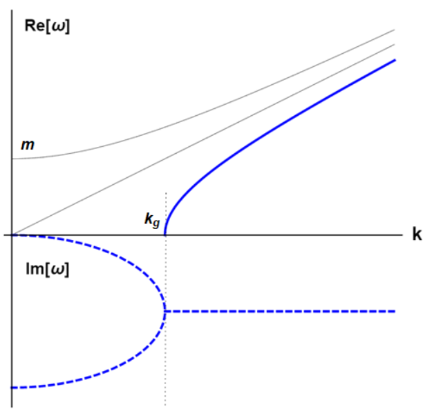
How large can the gap in (7) get? In condensed matter systems and liquids in particular, is limited by the UV scale: the interatomic separation and corresponding point comparable to . This can be seen in (7) by using the shortest value of comparable to the Debye vibration period . Using in (7) gives the maximal value of as , where we used . This corresponds to the shortest wavelength in the system to be , as expected on general grounds. In this picture, the size of the -gap must be smaller than the UV cutoff of the theory to have a well defined elastic regime where shear waves propagate.
We note that in liquids depends on pressure and temperature. Hence the condition giving the maximal gives a well-defined line on the phase diagram. This line is the Frenkel line (FL) separating the combined oscillatory and diffusive molecular motion from purely diffusive motion Trachenko and Brazhkin (2015); Brazhkin and Trachenko (2012); Brazhkin et al. (2013). The FL corresponds to qualitative changes of system properties in liquids and supercritical fluids and is ultimately related to the UV cutoff. Close to the FL, where the -gap is maximal, liquids acquire an interesting universality of properties: for example, the liquid viscosity becomes minimal and represents a universal quantum property governed by fundamental physical constants only Trachenko and Brazhkin (2020) which seems at work even in exotic states of matter such as the quark gluon plasma Trachenko et al. (2020).
Differently from liquids, increases without bound in scale-free field theories discussed below due to the absence of an UV regulator. In these theories, the UV cutoff and the Frenkel line do not exist.
III Two-field Lagrangian, its solutions and properties
III.1 Two-field Lagrangian
An important question from the field-theoretical perspective is what Lagrangian gives the spectrum given by Eq. (6) and the associated GMS? The challenge is to represent the viscous term in (2) in the Lagrangian. The viscous energy can be written as the work done to move the liquid. If is the strain, , where is the viscous force . Hence, the dissipative term in the Lagrangian should contain the term . This can be represented by a scalar field , giving the term . However, the term disappears from the Euler-Lagrange equation because . Another way to see this is note that the viscous term is simply a total derivative, .
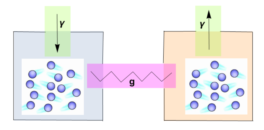
To circumvent this problem, we proposed to operate in terms of two fields and Trachenko (2017a, 2019). We note that a two-coordinate description of a localised damped harmonic oscillator was discussed earlier Bateman (1931); Dekker (1981). Two fields also emerge in the Keldysh-Schwinger approach to dissipative effects, describing an open system of interest and its environment (bath) Baggioli et al. (2020).
We constructed the dissipative term as the antisymmetric combination of Trachenko (2017a), namely as
| (8) |
Taking into consideration this new term, the Lagrangian density involving two scalar fields and and the dissipative term (8) reads Trachenko (2017a):
| (9) |
where we consider only one spatial direction for simplicity.
The scalar fields are real, and we verify the existence of real solutions later in this section. In real space, hermiticity or self-adjointness coincide with the invariance under the transposition operator since complex conjugation acts trivially. Defining the vector , we can write down the Lagrangian as:
| (10) |
where indicates the transposition operation. Then, the Lagrangian in Eq. 9 is not Hermitian in the sense that . However, we will see later than the Lagrangian (9) is symmetric.
Applying the Euler-Lagrange equations to (9) gives two decoupled equations for and :
| (11) |
where the equation for is the same as (2).
These equations have different solutions depending on whether is above or below . For , the most general form of physically relevant real solutions of (11) is:
| (12) |
where is the phase shift and where
| (13) |
has the form of (6) predicting the GMS.
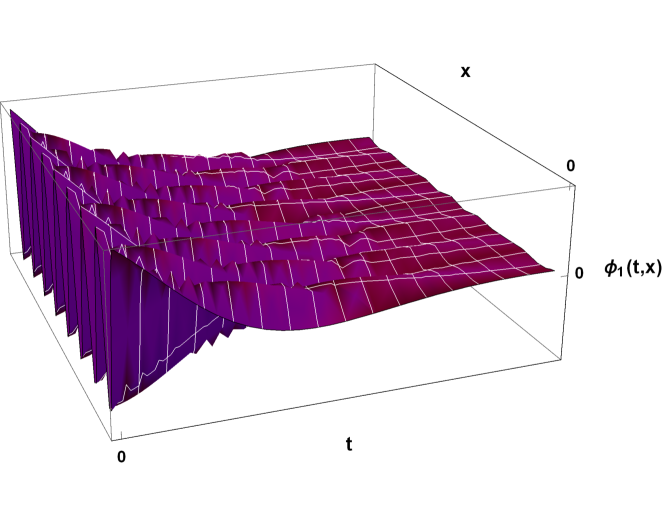
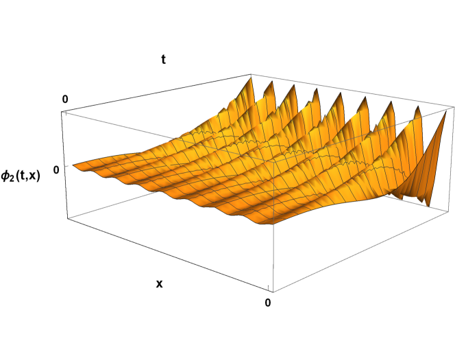
The solutions are shown in Fig. 2.
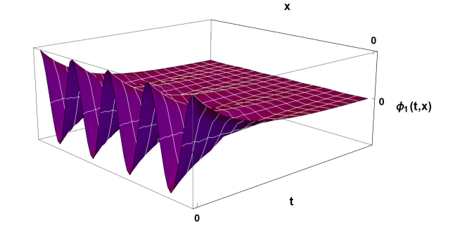
In the fluid regime111By ”fluid regime” we mean the range below where no propagating waves appear. Note that the “fluid regime” does not correspond to the hydrodynamic regime stricto sensu. The second regime needs both the frequency and momentum to be small and accounts for a single diffusive mode in the spectrum, as compared to two modes found at . In this second definition, hydrodynamics, intended as a perturbative EFT in small gradients, is different from fluid dynamics or fluid mechanics Landau and Lifshitz (2013b). Indeed, it can be applied also to solid systems and crystals Martin et al. (1972); Ammon et al. (2020)., , where no transverse modes propagate, the real solutions are:
| (14) | |||
| (15) |
These solutions are not periodic in time as illustrated in Fig.3 but respectively decay and grow exponentially.
The time dependence of and in (12) can be interpreted as energy exchange between waves and : and appreciably decrease and grow over time , respectively. This process is similar to the phonon scattering in crystals due to defects or anharmonicity where a plane-wave phonon () decays into other phonons (represented by ) and acquires a finite lifetime as a result. After the next time interval , the newly created phonon decays itself, transferring the energy to other phonons, and the process repeats. The time scale over which we consider and describe the dissipation process in (12) is because the phonon with the -gap dissipates after time comparable to (5).
This energy exchange can be represented by a generic approach to dissipation where the Lagrangian is written as Endlich et al. (2013):
| (16) |
The interaction term in (16) represents dissipation as the energy transfer from the degrees of freedom ”” to the degrees of freedom ””. We keep track of the degrees of freedom ”” related to dissipation but not the degrees of freedom ””, either because they are not of interest or are too complicated to account for. couples the two sectors and represent the energy exchange between them.
In the language of theories studying the open systems and non-Hermitian Hamiltonians (see next section), and in (12) are analogous to the “loss” and “gain” subsystems of a composite system Bender (2018), although in our case these subsystems are propagating waves suited for field-theoretical description rather than localised oscillators discussed earlier.
The parameters and in the dispersion relation (13) are subject to UV cutoffs in condensed matter phases, including in liquids where GMS emerge as discussed in the previous section. The high-temperature limit of is given by the shortest time scale in the system on the order of Debye vibration period . When , , or , where is the inter-particle separation and is Debye wavevector. Therefore, the limits of and at the UV cutoff are
| (17) |
The limits (17) apply to the field theory describing condensed matter phases with a well-defined UV regulator, e.g. lattice spacing. More generally, the field theory discussed here may involve UV cutoffs of different nature depending on the physical object it describes.
III.2 An alternative formulation of the two-field Lagrangian
In this section, we further elaborate on the origin of the dissipative Lagrangian discussed in the previous section. This will enable us to make a correspondence with the effective Lagrangian emerging in the Keldysh-Schwinger formalism discussed in the next section.
The first two cross terms in our initial Lagrangian (9) follow from the standard scalar field theory
| (18) |
using the standard transformation:
| (19) |
In terms of the fields and , the Lagrangian (9) reads
| (20) |
We note that in terms of fields, the non-hermiticity of Lagrangian (20) has a more standard meaning of .
Applying the Euler-Lagrange equations to (23) gives two coupled equations for and as
| (21) |
These equations can be de-coupled by using the same transformation (19): using (19) in (21) gives the system of two equations for and . Adding and subtracting these equations gives (11).
The solutions of (20) and (21) are generally complex. Representing these fields in the Lagrangian can be done using complex field conjugates Alexandre et al. (2019, 2017). However, this introduces an ambiguity in the equations of motion derived by applying the Euler-Lagrange equations to the Lagrangian. The ambiguity can be removed by selecting the solutions related by symmetry Alexandre et al. (2019, 2017) (see next section).
We note that taking real solutions and in (12), together with (19), implies that is real and is purely imaginary. In order to have a clearer formulation of our field theory, we continue our Lagrangian formulation in terms of real fields, similarly to (12) and define new real fields and as and . Then, (19) becomes
| (22) |
where all the fields involved in this transformation are real valued.
In the next section, we will see that this transformation is the same as the “Keldysh rotation” used in the Keldysh-Schwinger formalism.
In terms of the fields , the Lagrangian (9) reads
| (23) |
The Hamiltonian based on (9) or (23) is non-Hermitian due to the presence of the anti-symmetric last term , but it is invariant (see Ref. Bender et al. (2005a) for a similar case). As compared to the free-field part of (20), the free term for in (23), , has the opposite sign. In the next section, we show that this is related to the result following from Keldysh-Schwinger formalism. The opposite sign is not an issue from the point of view of system’s energy because the kinetic matrix is not diagonal due to the coupling . As explicitly shown in the next section, the system is stable and the Hamiltonian has a well-defined lower bound.
For , the solutions are
| (25) |
In the limit , according to (24). Hence, in the absence of dissipation, we have
| (26) |
In this case, the Lagrangian (23) becomes the free-field Lagrangian for the single field . Using in (22) also implies that , and the Lagrangian (9) similarly becomes the free-field Lagrangian for the single field .
This is an important point for two reasons. First, it shows that the number of degrees of freedom is halved in the absence of dissipation at . The meaning of the additional degree of freedom will become clear in the Keldysh-Scwhinger formalism in section III.3. Second, the remaining single degree of freedom is a plane wave with the dispersion relation . This ensures that the system reduces to the canonical situation in the limit .
III.3 The Lagrangian from Keldysh-Schwinger formalism
In the previous sections, we discussed how describing dissipation necessitates a two-field Lagrangian. We have earlier noted that the Keldysh-Schwinger (KS) formalism similarly involves two fields, and that the Green function operator contains the first time derivative which can be related to GMS Baggioli et al. (2020). Here, we make a stronger and more specific assertion. We show that two new important features of our dissipative Lagrangian (23) and emerging GMS appear in the KS formalism: (a) the new dissipative term of the form (8), and (b) the opposite sign of the free-field term of in (third and fourth terms in (23)).
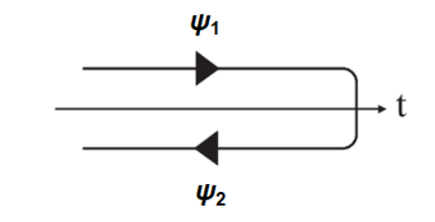
The description of non-equilibrium effective field theories involves the doubling of the degrees of freedom Liu and Glorioso (2018). Let us consider the simple case of one scalar field, . The action of a dissipative system depends on the initial state of the system and, accordingly, on the choice of initial time. The averaging operation is not defined in this case and, as a consequence, the statistical theory can not be formulated. To get around this problem, the KS formalism uses the following approach: consider a copy of our system with the same transition amplitude and the field in the replica system . Recall that both fields are identical, hence . Using these two fields, we reverse (invert) time in the second system and close the integration contour at . Then we can write the system’s path integral as
| (27) |
where are source terms associated with fields .
Importantly, the term related to the copy has the opposite sign, meaning that it propagates backward along the Keldysh-Schwinger contour Kamenev (2011a); Liu and Glorioso (2018). Therefore, we can interpret the field as the additional degree of freedom required to describe an open system and whose dynamics is reversed with respect to the arrow of time (see Fig. 4).
The KS formalism involves introducing , variables (retarded/advanced), defined as:
| (28) |
where variable is related to the real field dynamics, and variable related to dissipation and quantum fluctuations. This is the same transformation as (22) which we used earlier to find the relation between fields and .
By comparing the KS tranformation with (22), we see that plays the role of which corresponds to dissipation. As we will later find, . This implies unitarity of our field theory, ensured by the invariance of the action Mannheim (2013).
We now make this more precise and elaborate on the details. Let us consider an out-of-equilibrium system represented by a continuous field whose energy dissipates with time. We assume that at , the system is out of equilibrium and is in the state . It evolves to its final state, with energy is . In order to describe the system’s non-equilibrium dynamics, we use the KS technique Kamenev (2011b). We first write the transition probability from the initial state to the final one as follows:
| (29) | |||
where is the field conjugated to , is the characteristic time and the Lagrangian is given by
For details of this derivation we refer the reader to Ref. Baggioli et al. (2020).
As discussed earlier, this probability depends on the initial state of the system and, accordingly, on the choice of the initial time. The averaging operation is not defined in this case and, as a consequence, the statistical theory can not be formulated. In order to get around this problem, the KS approach Kamenev (2011b) introduces a copy of the system with the same transition probability. We denote the field in the initial system as and in the copy as . This is the same field, hence . Using the two fields, we close the integration contour in point (see Fig. 4) and write
After the Wick rotation , we obtain
Therefore, the effective Lagrangian of the theory is given by
| (30) | ||||
We now perform Keldysh rotation:
| (31) |
which is the same transformation we used earlier (22), and find
| (32) |
where we use the commutation relation for bosonic operators and note that .
Setting , we observe that (32) coincides with the dissipative Lagrangian we started with in (9) (up to a factor of 2 in front of ).
It is remarkable that the dissipative Lagrangian (9) and, therefore, the gapped momentum states effect appear to be related to a mature technique such as Keldysh-Schwinger formalism. We note an important caveat of this relation. The KS formalism does not contain the relaxation time . Instead, the timescale in the KS approach is set by the Planck constant. We have introduced as the relaxation time of the system on top of the standard KS formulation Baggioli et al. (2020), similarly to how is introduced in the Maxwell-Frenkel interpolation in (1)-(2), where it is assigned the meaning of the time between molecular rearrangement in the liquids Frenkel (1955). In this sense, Lagrangian (30) is not a derivation of our dissipative Lagrangian (23) from the KS formalism. However, it backs up two new and important features of our dissipative Lagrangian (23). First, it contains the term of the form . This is the same term (8) featuring in our Lagrangians (9) and (23) which is required to obtain GMS and which enters with the time scale set by . Second, the third and fourth terms describing the free-field contribution of the second field enter (30) with the sign opposite to that of the first field: . This is the same as in our dissipative Lagrangian (23).
III.4 The Hamiltonian
The Hamiltonian of our composite system consisting of fields and is
| (33) |
where is given in (9) and where the conjugate momenta are
| (34) |
This gives
| (35) |
The terms with re-appear in the Hamiltonian once the Hamiltonian is written in terms fields and momenta, as discussed in the next section.
We now compute the energy of our system directly using the solutions derived in the previous sections. The results are obviously independent of the choice of variables such as or .
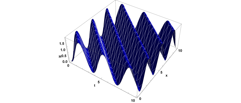
Using the solutions for in (12), the Hamiltonian for above the -gap is
| (36) |
Below the -gap, we have:
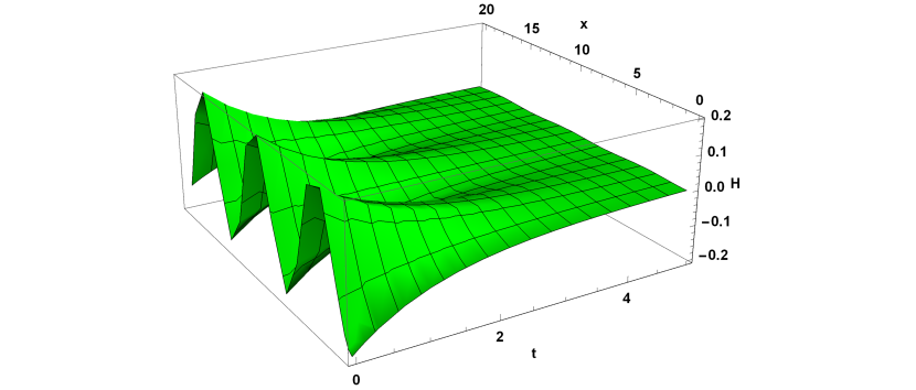
| (37) |
At , , and the two results coincide:
| (38) |
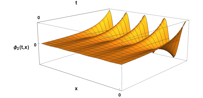
The Hamiltonian is displayed in Fig. 5 in both regimes. The Hamiltonian oscillates both in time and space for and decays with time for .
The lower bound of (36) is , or , according to (13). The lower limit of (37) is . Given that in this regime, of (37) is . Combined with from (13), the lower bound of (37) is , the same as the lower bound of (36). Therefore, has a finite value in both regimes for a finite . We recall that the UV cutoff for in condensed matter systems is given by in (17). The limit corresponds to the infinite gap and, therefore, non-propagating waves which our Lagrangian formulation is not designed to describe.
in agreement with the earlier calculation Trachenko (2017a), and
| (40) |
(40) is consistent with the fact that there are no propagating waves below the -gap.
To summarise, we find that the Hamiltonian of the composite gain-loss system is stationary in the propagating wave regime . In this regime, the energy has a lower bound and a positive average value. In the non-propagating regime , the system energy similarly has a lower bound and zero average energy as expected.
IV Non-Hermiticity and symmetry
As mentioned earlier, the Lagrangian of our theory, (9) or (23), is not Hermitian. However, we will see that both the Lagrangian and Hamiltonian in our theory are symmetric. We first recall how non-Hermiticity arises in theoretical approaches to dissipation.
The effect of dissipation can be generally represented by a complex energy spectrum, with imaginary term setting the lifetime of the state (see, e.g., Sudarshan et al. (1978); Sudarshan (2010); Rotter and Bird (2015); Rotter (2009)). This is similarly discussed in the context of resonances (see Ref. Feinberg (2011) for a recent discussion and a review) in which the complex energy plane is considered. Resonances are derived from complex poles of the form:
| (41) |
which necessitates a non-Hermitian model. The width of the resonances or, equivalently, their lifetime, is due to dissipation.
To illustrate how non-Hermiticity is related to dissipation and a finite relaxation time, it is instructive to consider a simple quantum mechanical system in the Heisenberg picture Chernodub and Cortijo (2019). Given a generic operator , its time dependence is given by:
| (42) |
The dynamics of such operator is:
| (43) |
We observe that a Hermitian Hamiltonian implies the conservation of this operator. On the contrary, the non-Hermiticity introduces a finite relaxation time:
| (44) |
The energy spectrum of a Hermitian Hamiltonian are real, however one of the central points of the discussion of symmetry under parity and time transformations ( symmetry) is that a Hermiticity can be replaced by a weaker condition: a non-Hermitian but -symmetric Hamiltonian may still result in real spectra. This follows from an assertion that -symmetric Hamiltonians have secular equations with real coefficients so that some of the eigenvalues can be real depending on parameters Bender (2018, 2007) 222It was observed that ”The reality of the spectrum of implies the presence of an antilinear symmetry (which is not necessarily ). Moreover, the spectrum of is real if and only if there is a positive-definite inner-product on the Hilbert space with respect to which is Hermitian or alternatively there is a pseudo-canonical transformation of the Hilbert space that maps into a Hermitian operator” Mostafazadeh (2002a, b, c)..
The discussion of the symmetry Bender (2018) starts with noting that a realistic physical system is an open non-isolated system with accompanying flux of probability flowing in or out. Theoretical description of this system is a long-standing problem, both classically and quantum-mechanically Davies (1976); Rotter and Bird (2015). The proposal to address this problem is to treat an open system as a subsystem and add another, time-reversed, subsystem with the opposite net flux of probability, so that the composite system had no net gain or loss of probability flux and is closed. The composite system exhibits the symmetry, where is the time-reversal operator and is the generic parity operator that interchanges the two subsystems Bender (2018).
Although the two subsystems are not stationary and are not in equilibrium separately, the stationary state of the composite system can be achieved by coupling the subsystems. The eigenvalues of the composite system are real, provided the coupling parameter is large enough, corresponding to the stationary state of the system and unbroken symmetry Bender (2018). This process can be illustrated by a system two coupled localised oscillators with gain and loss discussed earlier (see Fig. 6). The equations of motions for two coupled oscillators are and , where and are coordinates, is the friction coefficient and is the coupling parameter. The coupling term enters the Hamiltonian as , and the total Hamiltonian is -symmetric. There are three regimes: weak, intermediate and strong coupling corresponding to no real solutions (frequencies), four real solutions and two real solutions, respectively. The state where all solutions are real corresponds to unbroken symmetry, whereas complex solutions correspond to broken symmetry Bender (2018).
There are several interesting similarities and differences between the above system discussed in the context of symmetry and the system in our theory. First, and describe fields, rather than localised oscillators and correspond to propagating waves in the solutions. This is required in order to describe the -dependence and gapped momentum states in particular. Second, the and in (12) can be viewed as two subsystems with opposite fluxes of probability, similarly to the discussion of symmetry above. Third, the coupling term between and ( and ) is different and involves the coupling between one field and the derivative of the other field (see Eqs. (8),(9) and (23)) rather than between the fields themselves as in the model used in the above discussion of -symmetry.
Let us look at the properties of our system in more detail. The easiest way is to define the doublet:
| (45) |
Parity and time reversal transformations act on the coordinates as:
| (46) |
Their action on the field doublet can be written in matrix form as:
| (47) |
The latter coincides with the statement that a transformation swaps the source and the sink Bender (2018), i.e. .
Given these definitions, we observe that the Lagrangians (9) and (23) are invariant under the transformations involving fields swapping and change of time sign and, therefore, are -invariant. However, a Lagrangian is not a physical observable (unlike a Hamiltonian), and its unclear whether the -symmetry of the Lagrangian is related to real energy spectrum. To study the energy spectra, we write the Hamiltonian (35) in terms of fields and momenta as
| (48) |
The transformation involves changing the sign of momenta and swapping two fields. We observe that this gives , implying that H in (48) is -symmetric and . However, this is not a sufficient condition to ensure real eigenvalues. The caveat is that the time reversal is an antilinear operator. Given the eigenvectors of the Hamiltonian and operators:
| (49) |
the two eigenvectors do not necessarily coincide:
| (50) |
This last criterion defines two different phases of the system (see Fig.7): the unbroken phase and the broken phase. The first is distinguished from the second by the fact that the two sets of eigenvectors are equivalent. This implies:
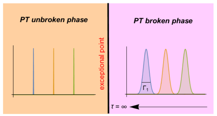
The second phase can be viewed as the phase where coupling between the source and the sink cannot be balanced Bender (2018), corresponding to a proper open system Rotter and Bird (2015); Davies (1976). The separation between the two phases is called the “exceptional point” and is characterized by interesting properties such as a the halving of the degrees of freedom and unparticle physics Heiss (2015); Zubkov (2012). In the context of non-Hermitian theories and dissipation, the exceptional point was discussed in Ref. Hashimoto et al. (2015).
The phase diagram of our system can be discussed using the eigenfrequencies of the system (4). They have the same form as (41):
| (51) |
The solutions of the form (51) are called “quasinormal modes” and are discussed in several fields, including dissipative open systems, holography Kovtun and Starinets (2005), hydrodynamics Kovtun (2012) and gravitational waves dynamics Nollert (1999); Chirenti (2018). In these areas, it is well recognised that the finite imaginary part of these modes determines the relaxation times of the excitations and governs the late-time dynamics of the physical system.
For a finite , our system is in the -broken phase because, according to Eq. (4), the spectrum always contains an imaginary term. The eigenvalues in our theory, given by Eq. (4), become real in the absence of dissipation and . This implies that corresponds to the exceptional point. Fig. (7) illustrates this point.
As discussed in section III, the number of degrees of freedom is halved in the absence of dissipation when . This is reminiscent of the exceptional point which separates the broken and unbroken phases. In our case, the exceptional point is at infinity and the system is always in the broken phase, in which the eigenvalues are complex.
V Correlation functions
Using Lagrangian (9), the equations of motion can be written in matrix form as:
| (52) |
where is the kinetic (matrix) operator, which in Fourier space is:
| (55) |
We define the matrix of Green’s functions as
| (56) |
with the inverse:
| (59) |
Then, the correlation functions read
| (60) | ||||
Taking the Fourier transform gives time dependence of these functions as
| (61) | ||||
where
| (62) |
is the frequency related to GMS as in (13).
To find the correlation functions for fields fields, we use the inverse transformation of (22):
resulting in
| (63) | ||||
Interestingly, the trace of the Green’s function matrix vanishes as follows from above and from (59): .
Taking the Fourier transform gives time dependence of these functions as
| (65) | ||||
For when is real and positive, the correlators of both fields and show a damped oscillatory behavior with two important features. First, the oscillation frequency of the correlation functions is set by in (62), the frequency that sets gapped momentum states as discussed throughout this paper. This frequency features in the poles of calculated correlation functions (see, e.g., Eqs. 61 and 65). Second, the decay time of the correlation functions is set by the relaxation time .
For in the fluid-mechanics regime, the oscillatory behaviour disappears, and the late time dynamics is exponentially decaying. This is illustrated in Fig. 8 where we plot the correlation function (65) in three different regimes.
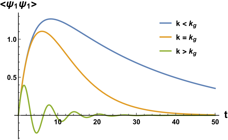
The behavior of correlation functions in (61) and (65) is expected and is physically reasonable. It shows that the non-Hermitian field theory with dissipation proposed here yields physically sensible results in terms of correlation functions and their frequency and time behavior. This is important in view of previous problems of formulating a Lagrangian-based field theory with dissipation.
The same results for correlation functions can be obtained using path integration. The path integral has the following form:
| (66) |
where is the functional measure, the four-momentum, is the coherence time and is the system’s volume in -space. If the Lagrangian has the form of (9) then
| (69) |
As a specific example, let us consider the calculation of the correlation function:
| (70) |
Using functional derivation, the correlation function can be written as
| (73) |
where and are the sources. After integrating over and , we obtain
| (74) |
This is the same result as in (60). The other correlators can be obtained using the same method. This shows that the path integral formulation of our theory is sensible and gives consistent results.
VI Interaction potential
We now address the behavior of the correlation functions in space. The Fourier transform of the propagator taken in space is related to the interaction potential between particles distance apart Zee (2003). The correlators in the presence of dissipation (60) depend on the modulus of and are rotationally invariant. Hence, the interaction potential depends on the radial coordinate only. In order to preserve the causality of the interactions, we choose the retarded correlator in (60), whose spatial Fourier transform is
| (75) |
Evaluating the integral in spherical coordinates gives
| (76) |
In the absence of dissipation , we recover the standard result Berestetskii et al. (2012)
| (77) |
Eq. (76) can be written as
| (78) |
where
| (79) | ||||
In the solid-like elastic propagating regime , , , and in Eq. (78) becomes
| (80) |
which is the same as Eq. (77) in the absence of dissipation.
In the non-propagating hydrodynamic regime , , and reads
| (81) |
in Eq. (81) differs from in (80) in two respects. First, the oscillating part in (81) can be viewed as the wave propagating with an effective frequency dependent speed
| (82) |
where in the regime .
Second, in (81), and therefore the corresponding interaction, become short-ranged and acquire an exponentially decreasing term , where the decay distance is
| (83) |
We observe that the wavelength in the oscillatory term in (81) is equal to the decay distance (83). Therefore, displays an overdamped dependence in -space in this regime, in contrast to Eq. (80).
The regime approximately coincides with (see Eq. (62)) and implies no propagating waves that mediate the interaction. It is therefore interesting that an interaction still operates and extends to a finite distance (83). This can be interpreted as follows. In the hydrodynamic regime , the hydrodynamic diffusive mode is
| (84) |
where is diffusion constant.
Eq. (83) gives
| (85) |
where we used (84).
Using , where is period, we find
| (86) |
which has the form of the Einstein diffusion equation.
Physically, this implies that despite the absence of propagating waves in the regime , the interaction is mediated by the diffusive mode up to a distance corresponding to the mean displacement in the Einstein relation. To the best of our knowledge, an interaction mediated by diffusive modes was not previously considered using formal field theory.
Eq. (83) implies that the decay distance becomes infinite in the limit of zero frequency. This corresponds to the mean displacement of the diffusive mode becoming infinite and interaction transmitted without exponential decay and screening.
VII Further discussion
VII.1 Departure from the “harmonic paradigm”
Introducing the quantum field theory and its Lagrangian , Zee writes Zee (2003):
| (87) |
The first two terms in (87) describe a harmonic theory and propagating plane waves, giving the starting point of the theory. The nonlinear terms describe scattering of plane waves originating from the harmonic part of the Lagrangian and production of new particles. The nonlinear terms need to be small compared to the harmonic term in order for the perturbation theory to converge and produce sensible results.
Zee observes Zee (2003) that the subject of the field theory remains rooted in this “harmonic paradigm”. Characterising this state of affairs as limited, he wonders about ways beyond the paradigm. Notably, our approach and in particular the Lagrangian (23) (or (9)) represents a departure from the harmonic paradigm in two important respects.
First, the elastic or harmonic (Klein-Gordon) term in (23) is not necessarily a starting point of the system description, with the viscous dissipative term added on top as is the case in the harmonic paradigm of the field theory based on (87). Indeed, both elastic and viscous term are treated in (23) on equal footing. The same applies to elastic and viscous terms in the Maxwell-Frenkel interpolation (1) where they are similarly treated on equal footing, and on which our Lagrangian formulation is based.
The combined effect of elastic and viscous terms is interestingly related to the widely-used term “viscoelasticity” and the area known as generalized hydrodynamics Boon and Yip (1991); Trachenko and Brazhkin (2015). The central effort in this area is to start with hydrodynamic equations such as Navier-Stokes equation and subsequently modify it to include the elastic response. The term and approach are related to the everyday observation that liquids flow and therefore necessitate a hydrodynamic approach as a starting point, with the elastic properties accounted for as a next step. However, we recently showed Trachenko (2017a) that the same Eq. (2) that follows from this Lagrangian can also be obtained by starting with a solid-like equation for a non-decaying wave and by subsequently generalizing the shear modulus to include the viscous response using Maxwell interpolation (1). Therefore, “elastoviscosity” is an equally legitimate term to describe Eq. (1) and (2) as well as Lagrangians (9) or (23). This is apparent in our Lagrangian (23) which gives no preference as to the starting point and treats elastic and viscous terms on equal footing.
Second and differently from (87) where nonlinear terms need to be small in order for the perturbation theory to converge, the dissipative term in (23) is not small in general. As discussed in the next section, large dissipative term (small ) results in purely hydrodynamic viscous regime where no shear waves propagate, completely negating the effect of the harmonic elastic term. In this sense, our approach and Lagrangian (23) is essentially non-perturbative.
The crossover to non-propagating regime is similar to the concept of diffusons which appears in the theory of electron-electron interactions in dirty metals Rammer (1998) as well as in physics of glasses and amorphous materials Allen et al. (1999); Baggioli and Zaccone (2019a, b).
Notably, we observe that all the nonlinear terms in (87) can be thought to be incorporated in the dissipative term in Lagrangian (23). At a deeper level, this is tantamount to stating that the introduction of liquid relaxation time by Frenkel Frenkel (1955) accounted for the (exponentially) complex problem of treating strongly-coupled nonlinear oscillators Trachenko and Brazhkin (2015); Trachenko (2017b).
VII.2 Implications for a Lagrangian formulation of hydrodynamics
As discussed earlier, the treatment of dissipative systems using a formal field theory has been a long-standing problem. A related open problem is formulating hydrodynamics, the area with a long history, using the field-theoretical description based on a Lagrangian. We note here that hydrodynamics in a broad sense is an effective field theory description valid at large wavelengths and long times. In this sense it is applicable to all systems, including crystals Martin et al. (1972). In a different context, “hydrodynamics” is used as an equivalent to “fluid-mechanics”and applies to liquids only Landau and Lifshitz (2013b). To avoid confusion, we will refer to hydrodynamics in a broad sense and to fluid dynamics in the second, more restrictive, sense.
One general approach to this problem was to use Keldysh-Schwinger-based techniques discussed earlier in this paper and out-of-time-order contours Grozdanov and Polonyi (2015); Liu and Glorioso (2018); Crossley et al. (2017); Jensen et al. (2018); Haehl et al. (2015) and more recently holography de Boer et al. (2019); Jana et al. (2020). Despite the action being typically non-Hermitian (i.e. containing a finite but positive imaginary part, ), a unitary evolution is ensured by the KMS constraint Liu and Glorioso (2018). In the regime where dissipation is slow, , an interesting phenomenological formalism (not derived from an action formalism) known as quasi-hydrodynamics Grozdanov et al. (2019) has been proposed and verified explicitly in several holographic constructions Baggioli et al. (2019b, a); Baggioli and Trachenko (2019b, a).
Our description of dissipation and gapped momentum states involves two fields in the Lagrangian (9) or (23) and in this sense is similar to the Keldysh-Schwinger approach where the two fields are introduced to close the integration contour (see section III.3). For convenience, we re-write (9) and (11):
| (88) |
| (89) | ||||
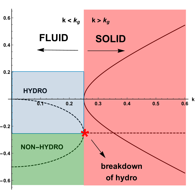
The Lagrangian and equations of motions have two parameters, and . This suggests that the Lagrangian can give rise to different regimes depending on and . Below we show that the constructed Lagrangian indeed has three well-defined regimes: (a) purely elastic non-dissipative and non-fluid regime, (b) mixed regime where transverse modes propagate above the -gap and (c) purely fluid-dynamics regime where no transverse modes propagate.
As discussed earlier, the most general solution describes propagating transverse modes above the -gap according to Eqs. (12) and (13). This is the mixed regime (b) above. The purely elastic Lagrangian, and regime (a) above, readily follows from setting , in which case , according to (12), and we are left with a standard propagating Klein-Gordon field. A non-propagating regime follows from considering the condition at which fluid mechanics applies: Frenkel (1955); Landau and Lifshitz (2013b). Considering time dependence of fields , we see that the terms with second and first time derivative in (89) are and , respectively. Therefore, the second time derivative term can be neglected in the regime , and we find the “loss” subsystem describing the Navier-Stokes equation predicting non-propagating waves, , and its gain counter-part, .
The different regimes also follow without bringing the frequency of external probe, , into consideration. The product of two parameters and in the Lagrangian (88) gives the length scale . We now recall that in the fluid mechanics regime, now transverse modes operate Landau and Lifshitz (2013b). It is easy to see our Lagrangian describes this regime at distance
| (90) |
Indeed, (88) results in no propagating modes when the frequencies (4) do not have a real part. This corresponds to , or for wavelengths (see Eq. (13)). We also recall that is the wave propagation range, and that a wave, in order to be well-defined, must not have a wavelength longer than the propagation range. Hence, (90) follows, as illustrated in Fig. 9.
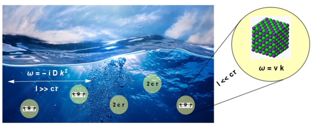
We note that hydrodynamics and fluid mechanics are often stated to describe the medium at small . The novelty here is that the field theory proposed gives a specific range of based on the parameters of the theory ( and ) where the fluid-mechanical description operates.
We note that conditions (90) and are consistent with the condition of applicability of fluid mechanics discussed earlier, . Indeed, combining the dispersion relation with the -gap (13) with gives , or approximately .
Increasing decreases the range of length scales where the hydrodynamic regime operates. At , this range shrinks to zero, consistent with removing the dissipative term in our lagrangian. On the other hand, small increases the hydrodynamic range. In this process, there is an interesting difference between the scale-free field theories and the field theory describing condensed matter phases with the UV cutoff. Unlike in scale-free field theories, can not decrease without bound in condensed matter phases and is bound by the shortest, Debye, vibration period, . When approaches , becomes and is approximately equal to the shortest distance in condensed matter phases set by the interatomic separation (see (17)).
It is interesting to recall that at the UV cutoff corresponds to the Frenkel line separating the combined oscillatory and diffusive components of liquid dynamics from purely diffusive motion Trachenko and Brazhkin (2015); Brazhkin and Trachenko (2012); Brazhkin et al. (2013). corresponds to approaching the zone boundary, at which point all transverse waves disappear from the system spectrum. This, in turn, corresponds to purely hydrodynamic Navier-Stokes solutions as discussed above.
We note that below the -gap, Eq. (4) gives two solutions. One of them is the diffusive mode representing the diffusive hydrodynamic shear flow:
| (91) |
The second mode is
| (92) |
and is not present in the standard formulation of fluid-mechanics description Landau and Lifshitz (2013b).
The second gapped mode is related to GMS, which emerges due to the collision between the diffusive and gapped modes. In a more general framework, this gapped mode can be captured by improved setups such as generalized hydrodynamics Grozdanov et al. (2019). The diffusive mode operates in the limit as in standard fluid mechanics, as is illustrated in Fig. 10.
VII.3 Implications for liquid theory
In addition to the general importance of formulating a field theory with dissipation, our results have more specific and practical interest in areas where decaying excitations are either experimentally measured or are obtained for modelling and need to fitted and analyzed. One example is the area of liquids where the measured inelastic structure factor needs to be fitted in order to extract phonon frequencies. Traditionally, the results of generalized hydrodynamics Boon and Yip (1991); Trachenko and Brazhkin (2015) are used to fit experimental spectra. Generalized hydrodynamics starts with the hydrodynamic equations and subsequently modifies them to account for solid-like non-hydrodynamic effects such as propagating transverse waves. Traditionally, this was supported by our experience that liquids flow and hence require a hydrodynamic theory as a starting point. However, more recent experiments show that even simple low-viscous liquids such as Na, Ga, Cu, Fe and so on are not hydrodynamic but, similarly to solids, support transverse waves with frequencies approaching the highest (Debye) frequency and wavelengths approaching the interatomic separation Trachenko and Brazhkin (2015). A hydrodynamic Navier-Stokes equation does not predict these waves Landau and Lifshitz (2013b); Frenkel (1955). Therefore, describing real liquids necessitates the presence of an elastic component in the equations of motion such as Eq. (2) which, in turn, follows from the viscoelastic Maxwell-Frenkel theory. As discussed earlier, this elastic component is manifestly present in the Lagrangian (23) in the form of the Klein-Gordon fields and enters the Lagrangian on equal footing with the hydrodynamic dissipative term. This discussion therefore revisits the point discussed in the earlier section related to the correct starting point of liquid description involving both hydrodynamic and elastic terms.
Returning to the generalized hydrodynamics approach, there are issues related to its phenomenological nature and, consequently, approximations used to fit liquid spectra Pilgrim and Morkel (2006); Giordano and Monaco (2010). These can affect the reliability and interpretation of experimental data. On the other hand, a Lagrangian formulation of combined effects of elasticity and dissipation is free from these complications. Moreover, the full range of field-theoretical methods can be applied to the Lagrangian to calculate different correlation functions of relevance in the liquid theory as well as other theories where dissipation plays a central role. In this respect, it is interesting to note that the functional form of the denominator of (64) is similar to that obtained in generalized hydrodynamics for correlation functions Boon and Yip (1991).
VIII Conclusions
In summary, we developed a field theory of dissipation based on gapped momentum states and using the non-Hermitian two-field theory with broken symmetry. The calculated correlation functions show decaying oscillatory behavior with the frequency and dissipation related to gapped momentum states. The interaction potential becomes short-ranged due to dissipation. We observed that the proposed field theory represents a departure from the harmonic paradigm theory and discussed the implications of this theory for the Lagrangian formulation of hydrodynamics.
Our theory is relatively simple as compared to more complicated setups Liu and Glorioso (2018) and is therefore suitable for practical and tractable calculations, providing an optimal formulation to study dissipation using field theory more generally and beyond the well-known phenomenological approaches. It would be interesting to extend our theory by adding new relevant fields and types of interaction and apply the theory to a wider range of systems of interest including, for example, electromagnetic and electron waves.
Acknowledgments
We are grateful to J. Alexandre, D. Arean, C. Bender, M. Chernodub, A. Cortijo, N. P. Fokeeva, S. Grozdanov, K. Landsteiner, N. Poovuttikul, K. Schalm and J. Zaanen for fruitful discussions and comments. K. T. thanks EPSRC for support. M. B. acknowledges the support of the Spanish MINECO’s “Centro de Excelencia Severo Ochoa” Programme under grant SEV-2012-0249.
References
- Landau and Lifshitz (2013a) L. Landau and E. Lifshitz, Statistical Physics, v. 5 (Elsevier Science, 2013).
- Rotter and Bird (2015) I. Rotter and J. Bird, Reports on Progress in Physics 78, 114001 (2015).
- Bender (2018) C. Bender, PT Symmetry: In Quantum and Classical Physics (World Scientific Publishing, 2018).
- Mohsen (2017) R. Mohsen, Classical And Quantum Dissipative Systems (World Scientific Publishing Company, 2017).
- Bender (2007) C. M. Bender, Reports on Progress in Physics 70, 947 (2007).
- Rotter (2009) I. Rotter, Journal of Physics A: Mathematical and Theoretical 42, 153001 (2009).
- Liu and Glorioso (2018) H. Liu and P. Glorioso, PoS TASI2017, 008 (2018), arXiv:1805.09331 [hep-th] .
- Kamenev (2011a) A. Kamenev, Field Theory of Non-Equilibrium Systems (Cambridge University Press, 2011).
- Endlich et al. (2013) S. Endlich, A. Nicolis, R. A. Porto, and J. Wang, Phys. Rev. D88, 105001 (2013), arXiv:1211.6461 [hep-th] .
- Crossley et al. (2017) M. Crossley, P. Glorioso, and H. Liu, JHEP 09, 095 (2017), arXiv:1511.03646 [hep-th] .
- Feynman and Vernon (1963) R. Feynman and F. Vernon, Annals of Physics 24, 118 (1963).
- Caldeira and Leggett (1981) A. O. Caldeira and A. J. Leggett, Phys. Rev. Lett. 46, 211 (1981).
- Weiss (1999) U. Weiss, Quantum Dissipative Systems, Series in modern condensed matter physics (World Scientific, 1999).
- Baggioli (2019) M. Baggioli, Applied Holography, Ph.D. thesis, Madrid, IFT (2019), arXiv:1908.02667 [hep-th] .
- Policastro et al. (2002) G. Policastro, D. T. Son, and A. O. Starinets, JHEP 09, 043 (2002), arXiv:hep-th/0205052 [hep-th] .
- Janik (2007) R. A. Janik, Phys. Rev. Lett. 98, 022302 (2007), arXiv:hep-th/0610144 [hep-th] .
- Baggioli and Trachenko (2019a) M. Baggioli and K. Trachenko, JHEP 03, 093 (2019a), arXiv:1807.10530 [hep-th] .
- Baggioli and Trachenko (2019b) M. Baggioli and K. Trachenko, Phys. Rev. D99, 106002 (2019b), arXiv:1808.05391 [hep-th] .
- Baggioli et al. (2019a) M. Baggioli, U. Gran, A. J. Alba, M. Tornsö, and T. Zingg, JHEP 09, 013 (2019a), arXiv:1905.00804 [hep-th] .
- Baggioli et al. (2019b) M. Baggioli, U. Gran, and M. Tornsö, (2019b), arXiv:1912.07321 [hep-th] .
- Trachenko and Brazhkin (2015) K. Trachenko and V. V. Brazhkin, Reports on Progress in Physics 79, 016502 (2015).
- Yang et al. (2017) C. Yang, M. T. Dove, V. V. Brazhkin, and K. Trachenko, Phys. Rev. Lett. 118, 215502 (2017).
- Trachenko (2017a) K. Trachenko, Phys. Rev. E 96, 062134 (2017a).
- Trachenko and Brazhkin (2014) K. Trachenko and V. Brazhkin, Journal of Physical Chemistry B 118, 11417 (2014).
- Baggioli and Zaccone (2019a) M. Baggioli and A. Zaccone, Phys. Rev. Lett. 122, 145501 (2019a).
- Baggioli et al. (2019c) M. Baggioli, R. Milkus, and A. Zaccone, Phys. Rev. E 100, 062131 (2019c).
- Baggioli and Zaccone (2019b) M. Baggioli and A. Zaccone, Phys. Rev. Research 1, 012010 (2019b).
- Baggioli and Zaccone (2020) M. Baggioli and A. Zaccone, Phys. Rev. Research 2, 013267 (2020).
- Baggioli et al. (2020) M. Baggioli, M. Vasin, V. Brazhkin, and K. Trachenko, Physics Reports (2020), https://doi.org/10.1016/j.physrep.2020.04.002.
- Zee (2003) A. Zee, Quantum Field Theory in a Nutshell (Princeton University Press, 2003).
- Maxwell (1867) J. C. Maxwell, Philosophical Transactions of the Royal Society of London 157, 49 (1867), https://royalsocietypublishing.org/doi/pdf/10.1098/rstl.1867.0004 .
- Frenkel (1955) J. Frenkel, Kinetic Theory of Liquids, Dover Publications (Dover, 1955).
- Dyre (2006) J. C. Dyre, Rev. Mod. Phys. 78, 953 (2006).
- Trachenko and Brazhkin (2009) K. Trachenko and V. V. Brazhkin, Journal of Physics: Condensed Matter 21, 425104 (2009).
- Feinberg (1967) G. Feinberg, Phys. Rev. 159, 1089 (1967).
- Brazhkin and Trachenko (2012) V. V. Brazhkin and K. Trachenko, Physics Today 65, 68 (2012), https://doi.org/10.1063/PT.3.1796 .
- Brazhkin et al. (2013) V. V. Brazhkin, Y. D. Fomin, A. G. Lyapin, V. N. Ryzhov, E. N. Tsiok, and K. Trachenko, Phys. Rev. Lett. 111, 145901 (2013).
- Trachenko and Brazhkin (2020) K. Trachenko and V. Brazhkin, Science Advances 6, eaba3747 (2020).
- Trachenko et al. (2020) K. Trachenko, V. Brazhkin, and M. Baggioli, (2020), arXiv:2003.13506 [hep-th] .
- Trachenko (2019) K. Trachenko, Scientific Reports 9, 6766 (2019).
- Bateman (1931) H. Bateman, Phys. Rev. 38, 815 (1931).
- Dekker (1981) H. Dekker, Physics Reports 80, 1 (1981).
- Landau and Lifshitz (2013b) L. Landau and E. Lifshitz, Fluid Mechanics, v. 6 (Elsevier Science, 2013).
- Martin et al. (1972) P. C. Martin, O. Parodi, and P. S. Pershan, Phys. Rev. A 6, 2401 (1972).
- Ammon et al. (2020) M. Ammon, M. Baggioli, S. Gray, S. Grieninger, and A. Jain, (2020), arXiv:2001.05737 [hep-th] .
- Alexandre et al. (2019) J. Alexandre, J. Ellis, P. Millington, and D. Seynaeve, Phys. Rev. D99, 075024 (2019), arXiv:1808.00944 [hep-th] .
- Alexandre et al. (2017) J. Alexandre, P. Millington, and D. Seynaeve, Phys. Rev. D96, 065027 (2017), arXiv:1707.01057 [hep-th] .
- Bender et al. (2005a) C. M. Bender, S. F. Brandt, J.-H. Chen, and Q.-h. Wang, Phys. Rev. D71, 025014 (2005a), arXiv:hep-th/0411064 [hep-th] .
- Mannheim (2013) P. D. Mannheim, Phil. Trans. Roy. Soc. Lond. A 371, 20120060 (2013), arXiv:0912.2635 [hep-th] .
- Kamenev (2011b) A. Kamenev, Field Theory of Non-Equilibrium Systems (Cambridge University Press, 2011).
- Sudarshan et al. (1978) E. C. G. Sudarshan, C. B. Chiu, and V. Gorini, Phys. Rev. D 18, 2914 (1978).
- Sudarshan (2010) E. G. Sudarshan, Progress of Theoretical Physics Supplement 184, 451 (2010), https://academic.oup.com/ptps/article-pdf/doi/10.1143/PTPS.184.451/5254474/184-451.pdf .
- Feinberg (2011) J. Feinberg, International Journal of Theoretical Physics 50, 1116 (2011).
- Chernodub and Cortijo (2019) M. N. Chernodub and A. Cortijo, (2019), arXiv:1901.06167 [cond-mat.mes-hall] .
- Mostafazadeh (2002a) A. Mostafazadeh, J. Math. Phys. 43, 205 (2002a), arXiv:math-ph/0107001 [math-ph] .
- Mostafazadeh (2002b) A. Mostafazadeh, J. Math. Phys. 43, 2814 (2002b), arXiv:math-ph/0110016 [math-ph] .
- Mostafazadeh (2002c) A. Mostafazadeh, J. Math. Phys. 43, 3944 (2002c), arXiv:math-ph/0203005 [math-ph] .
- Davies (1976) E. Davies, Quantum theory of open systems (Academic Press, 1976).
- Heiss (2015) W. D. Heiss, International Journal of Theoretical Physics 54, 3954 (2015).
- Zubkov (2012) M. A. Zubkov, Phys. Rev. D 86, 034505 (2012).
- Hashimoto et al. (2015) K. Hashimoto, K. Kanki, H. Hayakawa, and T. Petrosky, Progress of Theoretical and Experimental Physics 2015, 023A02 (2015).
- Kovtun and Starinets (2005) P. K. Kovtun and A. O. Starinets, Phys. Rev. D72, 086009 (2005), arXiv:hep-th/0506184 [hep-th] .
- Kovtun (2012) P. Kovtun, Lectures on hydrodynamic fluctuations in relativistic theories, J. Phys. A45, 473001 (2012), arXiv:1205.5040 [hep-th] .
- Nollert (1999) H.-P. Nollert, Class. Quant. Grav. 16, R159 (1999).
- Chirenti (2018) C. Chirenti, Black hole quasinormal modes in the era of LIGO, Braz. J. Phys. 48, 102 (2018), arXiv:1708.04476 [gr-qc] .
- Alexandre et al. (2018a) J. Alexandre, P. Millington, and D. Seynaeve, , J. Phys. Conf. Ser. 952, 012012 (2018a), arXiv:1710.01076 [hep-th] .
- Alexandre et al. (2018b) J. Alexandre, J. Ellis, P. Millington, and D. Seynaeve, Phys. Rev. D98, 045001 (2018b), arXiv:1805.06380 [hep-th] .
- Bender et al. (2005b) C. M. Bender, H. Jones, and R. Rivers, Physics Letters B 625, 333 (2005b).
- Berestetskii et al. (2012) V. Berestetskii, L. Pitaevskii, and E. Lifshitz, Quantum Electrodynamics: Volume 4, v. 4 (Elsevier Science, 2012).
- Boon and Yip (1991) J. Boon and S. Yip, Molecular Hydrodynamics, Dover books on physics (Dover Publications, 1991).
- Rammer (1998) J. Rammer, Quantum Transport Theory, Frontiers in physics (Perseus Books, 1998).
- Allen et al. (1999) P. B. Allen, J. L. Feldman, J. Fabian, and F. Wooten, Philosophical Magazine B 79, 1715 (1999), https://doi.org/10.1080/13642819908223054 .
- Trachenko (2017b) K. Trachenko, Phys. Rev. D 95, 043522 (2017b).
- Grozdanov and Polonyi (2015) S. Grozdanov and J. Polonyi, Phys. Rev. D91, 105031 (2015), arXiv:1305.3670 [hep-th] .
- Jensen et al. (2018) K. Jensen, R. Marjieh, N. Pinzani-Fokeeva, and A. Yarom, SciPost Phys. 5, 053 (2018), arXiv:1804.04654 [hep-th] .
- Haehl et al. (2015) F. M. Haehl, R. Loganayagam, and M. Rangamani, Phys. Rev. Lett. 114, 201601 (2015), arXiv:1412.1090 [hep-th] .
- de Boer et al. (2019) J. de Boer, M. P. Heller, and N. Pinzani-Fokeeva, JHEP 05, 188 (2019), arXiv:1812.06093 [hep-th] .
- Jana et al. (2020) C. Jana, R. Loganayagam, and M. Rangamani, (2020), arXiv:2004.02888 [hep-th] .
- Grozdanov et al. (2019) S. Grozdanov, A. Lucas, and N. Poovuttikul, Phys. Rev. D99, 086012 (2019), arXiv:1810.10016 [hep-th] .
- Pilgrim and Morkel (2006) W.-C. Pilgrim and C. Morkel, Journal of Physics: Condensed Matter 18, R585 (2006).
- Giordano and Monaco (2010) V. M. Giordano and G. Monaco, Proceedings of the National Academy of Sciences 107, 21985 (2010), https://www.pnas.org/content/107/51/21985.full.pdf .