Density dynamics in the mass-imbalanced Hubbard chain

Abstract

We consider two mutually interacting fermionic particle species on a one-dimensional lattice and study how the mass ratio $\eta$ between the two species affects the (equilibration) dynamics of the particles. Focussing on the regime of strong interactions and high temperatures, two well-studied points of reference are given by (i) the case of equal masses ${\eta=1}$, i.e., the standard Fermi-Hubbard chain, where initial non-equilibrium density distributions are known to decay, and (ii) the case of one particle species being infinitely heavy, ${\eta=0}$, leading to a localization of the lighter particles in an effective disorder potential. Given these two opposing cases, the dynamics in the case of intermediate mass ratios ${0<\eta<1}$ is of particular interest. To this end, we study the real-time dynamics of pure states featuring a sharp initial non-equilibrium density profile. Relying on the concept of dynamical quantum typicality, the resulting non-equilibrium dynamics can be related to equilibrium correlation functions. Summarizing our main results, we observe that diffusive transport occurs for moderate values of the mass imbalance, and manifests itself in a Gaussian spreading of real-space density profiles and an exponential decay of density modes in momentum space. For stronger imbalances, we provide evidence that transport becomes anomalous on intermediate time scales and, in particular, our results are consistent with the absence of strict localization in the long-time limit for any ${\eta>0}$. Based on our numerical analysis, we provide an estimate for the “lifetime” of the effective localization as a function of $\eta$.

I Introduction

Understanding the dynamics of quantum many-body systems is a central objective of modern physics which has been reignited by experimental advancements featuring, e.g., cold atoms or trapped ions Bloch et al. (2012); Blatt and Roos (2012), and has experienced an upsurge of interest also from the theoretical side Polkovnikov et al. (2011); Eisert et al. (2015); D’Alessio et al. (2016); Gogolin and Eisert (2016); Borgonovi et al. (2016). In this context, an intriguing and fundamental direction of research is to explain if and how thermodynamic behavior can emerge from the unitary time evolution of isolated quantum systems. One notable explanation for this occurrence of thermalization is the eigenstate thermalization hypothesis (ETH) Deutsch (1991); Srednicki (1994); Rigol et al. (2008), which has been numerically verified in numerous instances D’Alessio et al. (2016).

However, despite thermalization certainly being a rather common observation, there are also classes of systems which generically evade to reach thermal equilibrium even at indefinitely long times. In particular, it has been realized early on by Anderson that non-interacting particles in one or two spatial dimensions localize for an arbitrarily weak disorder potential Anderson (1958); Abrahams et al. (1979) (for experimental confirmations see, e.g., Roati et al. (2008); Billy et al. (2008)). Moreover, it is now widely believed that for sufficiently strong disorder, localization is also possible in the presence of interactions Nandkishore and Huse (2015); Abanin et al. (2019), which is supported by experimental results as well Schreiber et al. (2015).

While the majority of studies on many-body localization (MBL) typically focus on one-dimensional and short-ranged models composed of, e.g., spin-$1/2$ degrees of freedom, there has been much effort recently to generalize the notion of MBL to a wider class of models Gopalakrishnan and Parameswaran (2020). This includes, e.g., systems which are weakly coupled to a thermal bath Lüschen et al. (2017), models with long-range interactions Smith et al. (2016) or degrees of freedom with higher spin $S>1/2$ Richter et al. (2019, 2020), as well as Hubbard models where the disorder only couples to either one of the charge or spin degrees of freedom Prelovšek et al. (2016); Kozarzewski et al. (2018).

A particularly interesting question is whether MBL can also occur in systems which are translational invariant, i.e., without any explicit disorder Carleo et al. (2012); De Roeck and Huveneers (2014a, b, 2015); Grover and Fisher (2014); Schiulaz and Müller (2014); Altman and Vosk (2015); Papić et al. (2015); Schiulaz et al. (2015); Hickey et al. (2016); Yao et al. (2016); Smith et al. (2017); Michailidis et al. (2018); Brenes et al. (2018); Sirker (2019). A convenient model to investigate this question is given by the mass-imbalanced Hubbard chain Schiulaz and Müller (2014); Grover and Fisher (2014); Gamayun et al. (2014); Altman and Vosk (2015); Jin et al. (2015); Sirker (2019). In this model, two mutually interacting particle species are defined on a one-dimensional lattice and exhibit different hopping amplitudes. Here, the imbalance is parametrized by the ratio $\eta$ between the two hopping strengths, ranging from ${\eta=0}$, where the heavy particles are entirely static, to ${\eta=1}$, where the hopping amplitudes are the same. On the one hand, in the balanced limit ${\eta=1}$, numerical evidence for diffusive Prosen and Žnidarič (2012); Karrasch et al. (2017); Steinigeweg et al. (2017a) (or superdiffusive Prosen and Žnidarič (2012); Ilievski et al. (2018)) charge transport has been found in the regime of high temperatures and strong interactions. On the other hand, for ${\eta=0}$, the static particle species creates an effective disorder potential which induces localization of the lighter particles Paredes et al. (2005); Andraschko et al. (2014); Zhao et al. (2016); Enss et al. (2017); Jin et al. (2015). In view of these two opposing cases, it is intriguing to study the dynamics in the regime of intermediate imbalances ${0<\eta<1}$. While genuine localization (i.e. on indefinite time scales) is most likely absent for any ${\eta>0}$ Yao et al. (2016); Sirker (2019), e.g., due to slow anomalous diffusion which ultimately leads to thermalization Yao et al. (2016), this does not exclude the possibility of interesting dynamical properties such as a “quasi-MBL phase” at short to intermediate times Yao et al. (2016).

In this paper, we scrutinize the impact of a finite mass imbalance ${0<\eta<1}$ from a different perspective by studying the real-time dynamics of pure states featuring a sharp initial non-equilibrium density profile. Relying on the concept of dynamical quantum typicality, the resulting non-equilibrium dynamics can be related to equilibrium correlation functions. Summarizing our main results, we observe that diffusive transport occurs for moderate values of the mass imbalance, and that it manifests itself in a Gaussian spreading of real-space density profiles and an exponential decay of density modes in momentum space. Moreover, for stronger imbalances, we find evidence that on the time and length scales numerically accessible, transport properties become anomalous, albeit we cannot rule out that normal diffusion eventually prevails at even longer times. Furthermore, our results are consistent with the absence of genuine localization for any ${\eta>0}$. In particular, we find that for smaller and smaller values of ${\eta>0}$, the resulting dynamics resembles the localized ${\eta=0}$ case for longer and longer time scales. However, we conjecture that this “lifetime” of effective localization always remains finite for a finite $\eta$.

This paper is structured as follows. After introducing the model in Sec. II, we give an introduction to the employed typicality approach, and the initial states and observables in Sec. III. We then present our results in Sec. IV and conclude with a discussion in Sec. V.

II Model

Figure 1: (Color online) Illustration of the imbalanced Fermi-Hubbard chain. Spin-$\uparrow$ and -$\downarrow$ particles with on-site interaction of strength $U$ and different hopping amplitudes $t_{\uparrow}$ and $t_{\downarrow}$. Diffusive broadening of the initially peaked spin-$\uparrow$ density profile is sketched as a possible scenario depending on the imbalance ratio ${\eta=t_{\downarrow}/t_{\uparrow}}$.

We study the Hubbard chain describing interacting spin-$\uparrow$ and -$\downarrow$ fermions on a one-dimensional lattice. The Hamiltonian for $L$ lattice sites with periodic boundary conditions (${L+1\equiv 1}$) reads

$$H=\sum\limits_{r=1}^{L}h_{r}$$ (1)

with local terms

$$h_{r}=-\sum_{\sigma=\uparrow,\downarrow} t_{\sigma}\left(c_{r\phantom{l}\negmedspace,\sigma}^{{\dagger}}c_{r+1,\sigma}^{\phantom{{\dagger}}}+\mathrm{h.c.}\right)$$ (2)

$$+ \,U\left(n_{r,\uparrow}-\frac{1}{2}\right)\left(n_{r,\downarrow}-\frac{1}{2}\right)\ ,$$

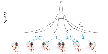
where the creation (annihilation) operator $c_{r,\sigma}^{{\dagger}}$ $(c_{r,\sigma})$ creates (annihilates) a fermion with spin $\sigma$ at site $r$, and ${n_{r,\sigma}=c_{r,\sigma}^{{\dagger}}c_{r,\sigma}^{\phantom{{\dagger}}}}$ is the particle-number operator. (We omit any additional operator symbols for the sake of clean notation.) The first term on the right hand side of Eq. (2) describes the site-to-site hopping of each particle species with amplitude $t_{\sigma}$. The second term is the on-site interaction between the particle species with strength $U$, see Fig. 1. The imbalance between $t_{\uparrow}$ and $t_{\downarrow}\leq t_{\uparrow}$ is parametrized by the ratio

$$\eta=\frac{t_{\downarrow}}{t_{\uparrow}}\ ,$$ (3)

ranging from ${\eta=0}$ for ${t_{\downarrow}=0}$ to ${\eta=1}$ in the case of ${t_{\downarrow}=t_{\uparrow}}$.

While the Hamiltonian $H$ in Eqs. (1) and (2) is integrable in terms of the Bethe Ansatz for ${\eta=1}$ (i.e. in the case of the standard Fermi-Hubbard chain, see, e.g., Ref. Essler et al. (2005)), this integrability is broken for any finite imbalance ${0<\eta<1}$. Moreover, despite its integrability, there has been numerical evidence that, in the regime of high temperatures and strong interactions, charge transport in the one-dimensional Fermi-Hubbard model is diffusive Prosen and Žnidarič (2012); Karrasch et al. (2017); Steinigeweg et al. (2017a) (or superdiffusive Prosen and Žnidarič (2012); Ilievski et al. (2018)). In order to have this well-controlled point of reference for our analysis of finite imbalances ${\eta\leq 1}$, we here fix the interaction strength to the large value ${U/t_{\uparrow}=16}$.

In addition to ${\eta=1}$, another important point in parameter space is the so-called Falicov-Kimball limit ${\eta=0}$ Falicov and Kimball (1969); Lyżwa and Domański (1994). In this limit, the spin-$\downarrow$ particles become completely immobile (${t_{\downarrow}=0}$), implying that the local occupation numbers $n_{r,\downarrow}$ become strictly conserved quantities, i.e.,

$$\left[H,n_{r,\downarrow}\right]=\left[n_{r,\downarrow},n_{r,\uparrow}\right]=0\ .$$ (4)

Using this symmetry, the Hamiltonian (1) can be decoupled into $2^{L}$ independent subspaces, effectively describing non-interacting spin-$\uparrow$ particles on a one-dimensional lattice with random (binary) on-site potentials ${\pm\,(U/2)\left(n_{r,\uparrow}-1/2\right)}$, which implies the onset of Anderson localization Anderson (1958).

It is worth mentioning that by means of a Jordan-Wigner transformation, the fermionic model in Eqs. (1) and (2) can be mapped to a spin-$1/2$ model with ladder geometry Yao et al. (2016). This spin model is described by the local terms

$$h_{r}=-\sum_{k=1,2} 2J_{k}\left(s_{r\phantom{l}\negmedspace,k}^{x}s_{r+1,k}^{x}+s_{r\phantom{l}\negmedspace,k}^{y}s_{r+1,k}^{y}\right)$$ (5)

$$+ \,J_{\bot}\,s_{r,1}^{z}s_{r,2}^{z}\$$

with ${J_{1}=t_{\uparrow}}$, ${J_{2}=t_{\downarrow}}$ and ${J_{\bot}=U}$. Here, the different particle species $\uparrow$ and $\downarrow$ are represented as local magnetizations on the two separate legs ${k=1,2}$ of the ladder. The hopping term and the interaction term in the Hubbard formulation correspond to the $XY$ interaction along the legs and the Ising interaction on the rungs of the ladder, respectively. The particle number conservation ${N_{\sigma}=\leavevmode\nobreak\ \sum_{r}n_{r,\sigma}=\leavevmode\nobreak\ \mathrm{const.}}$ for both particle types translates into magnetization conservation ${M_{k}=\leavevmode\nobreak\ \sum_{r}s^{z}_{r,k}=\leavevmode\nobreak\ \mathrm{const.}}$ on each leg.

III Setup and numerical method

III.1 Initial states and observables

We investigate the real-time dynamics of local particle densities given by the expectation values

$$p_{r,\sigma}(t)=\mbox{Tr}\left[\,{n_{r,\sigma}\rho(t)}\,\right]$$ (6)

with the density matrix

$$\rho(t)=\mathrm{e}^{-\mathrm{i}Ht}\ket{\psi(0)}\bra{\psi(0)}\mathrm{e}^{\mathrm{i}Ht}$$ (7)

for pure initial states $\ket{\psi(0)}$, such that

$$\mbox{Tr}\left[\,{n_{r,\sigma}\rho(t)}\,\right]=\bra{\psi(t)}n_{r,\sigma}\ket{\psi(t)}\ .$$ (8)

In order to realize inhomogeneous particle densities, we prepare the initial states via the projection

$$\ket{\psi(0)}\propto n_{L/2,\uparrow}\ket{\phi}\ .$$ (9)

The reference pure state $\ket{\phi}$ is constructed as a random superposition,

$$\ket{\phi}=\sum\limits_{k=1}^{d}c_{k}\ket{\varphi_{k}}\ ,$$ (10)

where the $\ket{\varphi_{k}}$ denote the common eigenbasis of the local occupation number operators $n_{r,\sigma}$, and the sum runs over the full Hilbert space with finite dimension ${d=4^{L}}$. (In spin language, this simply is the Ising basis.) Moreover, the complex coefficients $c_{k}$ are randomly drawn from a distribution which is invariant under all unitary transformations in the Hilbert space (Haar measure) Bartsch and Gemmer (2009, 2011), i.e., real and imaginary parts of these coefficients are normally distributed with zero mean. As a consequence, the initial density profile exhibits a sharp delta peak for the spin-$\uparrow$ particles in the middle of the chain on top of a homogeneous many-particle background Steinigeweg et al. (2017a, b),

$$p_{r,\sigma}(0)\ \begin{cases}\quad=\phantom{1}1&r=L/2\ \mathrm{and}\ \sigma=\ \uparrow\\ \quad\approx 1/2=p_{\mathrm{eq.}}&\mathrm{else}\end{cases}\ .$$ (11)

Rather than taking the full Hilbert space into account, one could also consider the half-filling sector (respectively the zero-magnetization sector).

III.2 Dynamical quantum typicality

Given the specific construction of the pure state $\ket{\phi}$ in Eq. (10), the concept of dynamical quantum typicality (DQT) provides a direct connection between the non-equilibrium expectation value $p_{r,\uparrow}(t)$ and an equilibrium correlation function (see Ref. Steinigeweg et al. (2017a) and also Appendix A),

$$p_{r,\uparrow}(t)-p_{\mathrm{eq.}}= \,2\braket{(n_{L/2,\uparrow}-p_{\mathrm{eq.}})(n_{r,\uparrow}(t)-p_{\mathrm{eq.}})}+\epsilon\ ,$$ (12)

where the thermodynamic average $\braket{\bullet}=\mbox{Tr}\left[\,{\bullet}\,\right]/d$ is carried out at formally infinite temperature. As a consequence, the dynamics of the non-equilibrium expectation value $p_{r,\uparrow}(t)$ can be used to study transport properties within the framework of linear response theory.

Importantly, the variance of the statistical error ${\epsilon=\epsilon(\ket{\phi})}$ of Eq. (12) is bounded from above by

$$\text{Var}(\epsilon)<\mathcal{O}\left(\frac{1}{d}\right)=\mathcal{O}\left(4^{-L}\right)\ ,$$ (13)

i.e., the accuracy of the typicality approximation improves exponentially upon increasing the size of the system. In principle, this error can be further reduced by averaging over multiple realizations of the random state $\ket{\phi}$ Schnack et al. (2020a, b). However, for the system sizes studied here, the DQT approach is already very accurate, and this additional sampling becomes unnecessary Heitmann et al. (2020). More details on the concept of dynamical quantum typicality (and on error bounds) can be found in Refs. Gemmer and Mahler (2003); Iitaka and Ebisuzaki (2003, 2004); Goldstein et al. (2006); Popescu et al. (2006); Reimann (2007); White (2009); Sugiura and Shimizu (2012, 2013); Elsayed and Fine (2013); Steinigeweg et al. (2014a, b); Monnai and Sugita (2014); Reimann (2016, 2018); Heitmann et al. (2020).

III.3 Time evolution via pure-state propagation

For the time evolution of the pure state

$$\ket{\psi(t)}=\mathrm{e}^{-\mathrm{i}Ht}\ket{\psi(0)}$$ (14)

we can bypass the exact diagonalization of the Hamiltonian and rather solve the time-dependent Schrödinger equation directly via iterative forward propagation in small time steps $\delta t$. Aside from the many numerical methods such as Trotter decompositions de Vries and De Raedt (1993); De Raedt and Michielsen (2006), Chebyshev polynomials Tal‐Ezer and Kosloff (1984); Dobrovitski and De Raedt (2003); Weiße et al. (2006) or Krylov-space methods Nauts and Wyatt (1983), the action of the time-evolution operator in each step can be calculated by a fourth-order Runge-Kutta scheme Elsayed and Fine (2013); Steinigeweg et al. (2014a),

$$\ket{\psi(t+\delta t)} =\mathrm{e}^{-\mathrm{i}H\delta t}\ket{\psi(t)}$$ (15)

$$\approx\sum\limits_{k=0}^{4}\frac{(-\mathrm{i}H\delta t)^{k}}{k!}\ket{\psi(t)}\ .$$

Crucially, the matrix-vector multiplications in Eq. (15) can be implemented very memory efficiently due to the sparse matrix representation of the given Hamiltonian. While the action of $H$ on $\ket{\psi}$ can also be calculated on-the-fly, we save the sparse Hamiltonian matrix for the sake of run time. Moreover, symmetries of the system can be exploited in order to split the problem into smaller sub-problems and to further reduce the computational effort Heitmann and Schnack (2019). In this paper, we exploit the particle number (magnetization) conservation for both particle species (legs) separately. As a consequence, the maximum memory consumption for the largest symmetry sector in a system of length ${L=15}$, with full Hilbert-space dimension ${d\sim 10^{9}}$, amounts to about $20$ GB (using double-precision complex numbers). While ${L=14}$ or ${L=15}$ are already comparatively large (especially in view of the extensive parameter screening and the long simulation times considered here), let us note that even larger system sizes can be treated by the usage of large-scale supercomputing (see, e.g., Refs. Jin et al. (2015); Steinigeweg et al. (2017a)). The time step used in all calculations, if not stated otherwise, is ${\delta t\,t_{\uparrow}=0.005}$.

III.4 Diffusion on a lattice

III.4.1 Real space

The dynamics of the densities $p_{r,\uparrow}(t)$ is diffusive, if it fulfills the lattice diffusion equation Bertini et al.

$$\frac{d}{dt}p_{r,\uparrow}(t)=D[p_{r-1,\uparrow}(t)-2p_{r,\uparrow}(t)+p_{r+1,\uparrow}(t)]$$ (16)

with the diffusion constant $D$. For the $\delta$-peak initial conditions (11), the solution of Eq. (16) can be well approximated by the Gaussian function

$$p_{r,\uparrow}(t)-p_{\mathrm{eq.}}=\frac{1}{2\sqrt{2\pi}\Sigma(t)}\exp\left[-\frac{(r-L/2)^{2}}{2\Sigma^{2}(t)}\right]\ ,$$ (17)

where the spatial variance scales as ${\Sigma^{2}(t)=2Dt}$ and is given by

$$\Sigma^{2}(t)=\sum\limits_{r=1}^{L}r^{2}\delta p_{r,\uparrow}(t)-\left[\sum\limits_{r=1}^{L}r\delta p_{r,\uparrow}(t)\right]^{2}\ ,$$ (18)

with ${\delta p_{r,\uparrow}(t)\propto p_{r,\uparrow}(t)-p_{\mathrm{eq.}}}$ fulfilling ${\sum_{r}\delta p_{r,\uparrow}(t)=1}$ for all times $t$. More generally, a scaling of the variance according to ${\Sigma(t)\propto t^{\alpha}}$ is called ballistic for ${\alpha=1}$, superdiffusive for ${1/2<\alpha<1}$, diffusive for ${\alpha=1/2}$, subdiffusive for ${0<\alpha<1/2}$, and localized for ${\alpha=0}$. Moreover, away from the case ${\alpha=1/2}$, the density profiles $p_{r,\uparrow}(t)$ are not expected to take on a Gaussian shape.

III.4.2 Connection to current-current correlation functions

Due to the typicality relation (12), the spatial variance in Eq. (18) can be related to the dynamics of current-current correlation functions via Steinigeweg et al. (2009)

$$\frac{d}{dt}\Sigma^{2}(t)=2D(t)\ ,$$ (19)

where the time-dependent diffusion coefficient $D(t)$ is given by

$$D(t)=\frac{4}{L}\int\limits_{0}^{t}\langle j_{\uparrow}(t^{\prime})j_{\uparrow}\rangle\,dt^{\prime}\ ,$$ (20)

and $j_{\uparrow}$ denotes the total current operator of the spin-$\uparrow$ particles,

$$j_{\uparrow}=-t_{\uparrow}\sum\limits_{r}\left(\ \mathrm{i}c_{r,\uparrow}^{{\dagger}}c_{r+1,\uparrow}^{\phantom{{\dagger}}}+\mathrm{h.c.}\right)\ .$$ (21)

(Note that the relation (19) requires $\delta p_{r,\uparrow}(t)$ to vanish at the boundaries of the chain Steinigeweg et al. (2009).) We therefore can compare the spatial variance of density profiles calculated according to Eq. (18) to the one already obtained from current-current correlation functions Steinigeweg et al. (2009); Yan et al. (2015); Karrasch et al. (2017),

$$\Sigma^{2}(t)=2\int\limits_{0}^{t}D(t^{\prime})dt^{\prime}\ .$$ (22)

A detailed analysis of transport in the mass-imbalanced Hubbard chain extracted from current-current correlation functions can be found in Jin et al. (2015).

III.4.3 Momentum space

In addition to the real-space perspective, it is also instructive to look at momentum-space observables as given by the lattice Fourier transform of the density profiles,

$$p_{q,\uparrow}(t)=\frac{1}{\sqrt{L}}\sum\limits_{r=1}^{L}\mathrm{e}^{\mathrm{i}qr}p_{r,\uparrow}(t)$$ (23)

with the momentum ${q=2\pi k/L}$ and wave numbers ${k=0,1,\dots,L-1}$. In particular, the Fourier transformation of the diffusion equation (16) yields the corresponding diffusion equation for the $p_{q,\uparrow}(t)$,

$$\frac{d}{dt}p_{q,\uparrow}(t)=-\widetilde{q}^{2}D\,p_{q,\uparrow}(t)\ ,$$ (24)

with ${\widetilde{q}^{2}=2(1-\cos q)}$. From Eq. (24), it becomes clear that diffusion manifests itself in momentum space by exponentially decaying modes

$$p_{q,\uparrow}(t)\propto\mathrm{e}^{-\widetilde{q}^{2}Dt}\ .$$ (25)

IV Results

We now turn to our numerical results. To begin with, the two limiting cases ${\eta=1}$ and ${\eta=0}$ are presented in Sec. IV.1. Intermediate imbalances ${0<\eta<1}$ are discussed in Secs. IV.2 and IV.3.

IV.1 Limiting cases

Figure 2: (Color online) Real-time broadening of the non-equilibrium density profile for limiting imbalance ratios (a) $\eta=1$ and (b) $\eta=0$. System size $L=14$ and interaction strength $U/t_{\uparrow}=16$. The initial density peak in the center of the chain spreads rather quickly over the system for $\eta=1$, whereas it appears to be frozen for $\eta=0$.

Figure 3: (Color online) Density profiles $p_{r,\uparrow}(t)$ at fixed times for (a) $\eta=1$ and (b) $\eta=0$. In the case $\eta=1$, the profiles can be very well described via Gaussians (parabola in the semi-logarithmic plot) indicating clean diffusion for the time scales depicted. Note that the Gaussians (dashed lines) are no fit, but calculated from Eqs. (17) and (18). In the case $\eta=0$, an overall triangular shape survives even for long times, with some local fluctuations.

In order to mark out the two completely different behaviors of the density dynamics in the limiting cases of the model, we first discuss the limit of equal particle masses ($\eta=1$) and contrast it with the limit of infinite mass-imbalance (${\eta=0}$). Recall that the interaction strength is set to ${U/t_{\uparrow}=16}$ in the following.

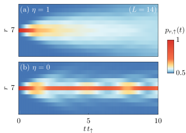
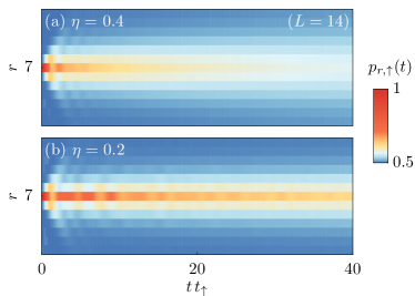
First, Fig. 2 shows the real-time broadening of the initially peaked density profiles $p_{r,\uparrow}(t)$ for both limits in a time-space density plot. While the particle density for $\eta=1$ [Fig. 2 (a)] is found to spread over all sites of the chain, $p_{r,\uparrow}(t)$ for $\eta=0$ [Fig. 2 (b)] appears to be essentially frozen at the central lattice sites, as it is expected in the Anderson insulating limit.

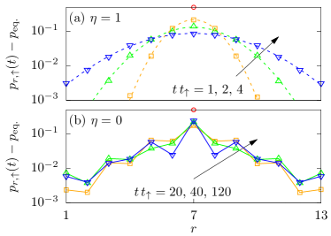
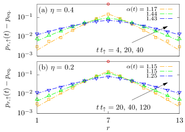
For a more detailed analysis, the spatial dependence of the profiles ${p_{r,\uparrow}(t)-p_{\mathrm{eq.}}}$ is shown in Fig. 3 for fixed times $t$ in a semi-logarithmic plot. Remarkably, the profiles for ${\eta=1}$ in Fig. 3 (a) can be very well described by Gaussians [see Eq. (17)] over three orders of magnitude. These Gaussian profiles indicate that charge transport in the integrable Fermi-Hubbard chain is diffusive Prosen and Žnidarič (2012); Karrasch et al. (2017); Steinigeweg et al. (2017a), at least in this parameter regime (strong interactions and high temperatures) and for the time scales depicted, see also Refs. Prosen and Žnidarič (2012); Ilievski et al. (2018) for the possibility of superdiffusive transport. Note that the Gaussians in Fig. 3 (a) are no fit, since the width $\Sigma(t)$ has been calculated exactly according to Eq. (18), i.e., there is no free parameter involved. In contrast, the profiles for ${\eta=0}$ in Fig. 3 (b) are clearly non-Gaussian and remain, even for the long times shown, in an overall triangular shape with variations on short length scales.

IV.2 Small imbalances

IV.2.1 Real space

Figure 4: (Color online) Real-time broadening of the initially peaked density profile for weak imbalances (a) $\eta=0.8$ and (b) $\eta=0.6$.

Figure 5: (Color online) Density profiles $p_{r,\uparrow}(t)$ at fixed times for the same system parameters and imbalance ratios as shown in Fig. 4. The dashed lines are Gaussian functions calculated from Eqs. (17) and (18). At moderate imbalance (a) ${\eta=0.8}$, the profiles can be very well described by Gaussians. At slightly smaller (b) ${\eta=0.6}$, the density profiles are still in good agreement with Gaussians, although small deviations become apparent at ${t\,t_{\uparrow}=4}$.

Next, let us study a finite imbalance between the particle masses. In analogy to Fig. 2, time-space density plots are shown in Fig. 4 for ${\eta=0.8}$ and ${\eta=0.6}$. For these ratios the broadening of the initial density peak apparently happens on a time scale comparable to the one observed for ${\eta=1}$ in Fig. 2, with a barely noticeable slowdown with the increasing imbalance. Similar observations can be made for the density profiles at fixed times, as shown in Fig. 5. At weak imbalance ${\eta=0.8}$ [Fig. 5 (a)], the profiles are still in very good agreement with Gaussians [see Eq. (17)] which suggests that diffusion occurs also for ${\eta\neq 1}$. Even for stronger imbalance ${\eta=0.6}$ [Fig. 5 (b)], the profiles appear to be of Gaussian shape, although small deviations start to appear at ${t\,t_{\uparrow}=4}$, which might be seen as the onset of a drift from normal to anomalous diffusion, see also the discussion below.

IV.2.2 Spatial width

Figure 6: (Color online) Spatial width $\Sigma(t)$ as obtained by Eq. (18) for imbalance ratio ${\eta=0.8}$ and different system sizes ${L=10,\dots,14}$ (arrow). The dotted line with the scaling $\Sigma(t)\propto\sqrt{t}$ is a fit to the $L=14$ curve. The width $\Sigma(t)$ (dashed-dotted line) as calculated by Eq. (22) is shown for comparison (${L=14}$).

In order to analyze the broadening of the density profiles further, Fig. 6 shows the time-dependence of the spatial width $\Sigma(t)$ obtained by Eq. (18) for moderate imbalance ${\eta=0.8}$ and different system sizes ${L=10,\dots,14}$. Necessarily, there is an initial linear increase ${\Sigma(t)\propto t}$ for ${t\,t_{\uparrow}\lesssim 1}$, indicating ballistic transport, as it is expected for short times below the mean-free time. Subsequently, $\Sigma(t)$ shows a scaling ${\propto\sqrt{t}}$, consistent with diffusion. However, for later times, we find that $\Sigma(t)$ approaches a saturation value which increases with increasing $L$. This behavior of $\Sigma(t)$ can be easily understood since the width of a density profile on a finite lattice with $L$ sites is obviously bounded from above. Namely, assuming equilibration, i.e., a perfectly homogeneous distribution of the $p_{r,\uparrow}$ for $t\rightarrow\infty$ with $\delta p_{r,\uparrow}=1/L$ at each site, we obtain the saturation value

$$\Sigma^{2}(t\rightarrow\infty) =\sum\limits_{r=1}^{L}\frac{r^{2}}{L}-\left[\sum\limits_{r=1}^{L}\frac{r}{L}\right]^{2}$$ (26)

$$=\frac{1}{12}\left(L^{2}-1\right)\ .$$

This $L$-dependent saturation value is reached quickly for the weakly imbalanced case ${\eta=0.8}$ in Fig. 6, e.g., ${\Sigma\approx 4}$ for ${L=14}$.

Moreover, for the biggest size ${L=14}$, Fig. 6 also shows $\Sigma(t)$ calculated from current-current correlation functions via Eq. (22). Overall, the behavior of this $\Sigma(t)$ is in good agreement with the one described above. Note that the small deviations between the two widths setting in at ${t\,t_{\uparrow}\sim 6}$ presumably arise when the tails of the density distribution reach the boundaries of the system (cf. Fig. 5). Additionally, we note that the finite-size saturation value (26) does not apply to Eq. (22), which, by definition, is not bounded. Rather, for times ${t\,t_{\uparrow}\gtrsim 6}$, we find an accelerated increase of $\Sigma(t)$. This is caused by the fact that the current-current correlation function ${\langle j_{\uparrow}(t)j_{\uparrow}\rangle}$ does not completely decay to zero in a system of finite size, see also Refs. Jin et al. (2015); Bertini et al. .

IV.2.3 Momentum space

Figure 7: (Color online) Discrete Fourier transform $p_{q,\uparrow}(t)$ of the density profile with momentum ${q=2\pi k/L}$ and wave numbers ${k=1,2,3,4}$ (arrow) for weak imbalances (a) ${\eta=0.8}$ and (b) ${\eta=0.6}$.

Complementary to the real-space data for ${\eta=0.8,0.6}$ shown in Fig. 5, the corresponding Fourier modes $p_{q,\uparrow}(t)$ with momentum ${q=2\pi k/L}$ are shown in Fig. 7 for the four longest wavelengths available, i.e., ${k=1,\dots,4}$. While $p_{q,\uparrow}(t)$ decays rather quickly for ${k\geq 2}$ (with the decay rate increasing with $k$), we find that at least for ${k=1}$, $p_{q,\uparrow}(t)$ is to good quality described by an exponential decay [see Eq. (25)], consistent with the onset of diffusion on the corresponding length scales.

IV.3 Strong mass imbalance

Now, let us study how the equilibration dynamics alter for stronger imbalances and also discuss the possibility of localization for ${\eta>0}$.

IV.3.1 Real-space dynamics

Figure 8: (Color online) Decay of the central peak $p_{L/2,\uparrow}(t)$ at different imbalances ranging from ${\eta=0}$ to ${\eta=1}$ (from top to bottom) for system sizes ${L=12}$ (dotted) and ${L=14}$ (solid). Dashed lines indicate the expected $L$-dependent long-time value $(1-p_{\mathrm{eq.}})/L$.

Figure 9: (Color online) Time-space density plot as in Fig. 4 but for (a) ${\eta=0.4}$ and (b) ${\eta=0.2}$.

Figure 10: (Color online) Density profiles $p_{r,\uparrow}(t)$ as in Fig. 5 but for smaller (a) ${\eta=0.4}$ and (b) ${\eta=0.2}$. The profiles broaden much slower and take on a triangular shape in the semi-logarithmic plot used. The fit parameter $\alpha(t)$ is the exponent used in Eq. (27).

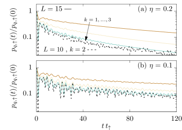
Before discussing the full density profile in detail, let us for simplicity focus on the decay of the central peak $p_{L/2,\uparrow}(t)$, as shown in Fig. 8 for imbalance ratios ${\eta=0,\dots,1}$ and two system sizes ${L=12}$ and ${L=14}$. While ${p_{L/2,\uparrow}(t)\propto t^{-1/2}}$ to good quality for $\eta=1$, consistent with diffusive transport, this decay is slowed down with decreasing $\eta$. At small but finite $\eta=0.1$, we find that $p_{L/2,\uparrow}(t)$ approximately coincides with the $\eta=0$ curve up to times ${t\,t_{\uparrow}\approx 40}$, until it eventually starts to decay towards the equilibrium value ${p_{L/2,\uparrow}(t\rightarrow\infty)-p_{\mathrm{eq.}}=(1-p_{\mathrm{eq.}})/L}$. Note that the two curves for ${L=12,14}$ agree very well with each other before the equilibration value is reached. On these time scales, the behavior of the density dynamics thus appears to be independent of the system size. This also illustrates the accuracy of the DQT approach, since there is no sign of sample-dependence in the time-dependent fluctuations of the strongly imbalanced curves. For additional data with smaller $\eta$ and longer time scales, see Appendix B. Moreover, a more detailed finite-size analysis can be found in Appendix C.

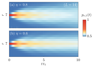
Next, let us come back to a discussion of the full density profile. To this end, Fig. 9 shows time-space density plots for the two ${\eta=0.4}$ and ${\eta=0.2}$. We find that the broadening of the density profiles visibly slows down with decreasing $\eta$, until no substantial spreading of the density can be observed for ${\eta=0.2}$ up to the maximum time ${t\,t_{\uparrow}=40}$ shown here, consistent with Fig. 8 discussed before.

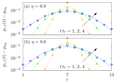
The corresponding cuts of the density profiles at fixed times are shown in Figs. 10 (a) and (b). Note that, owing to the slow broadening of the profiles, we show cuts at later times compared to Fig. 5. One clearly sees that the profiles are not Gaussian anymore, but rather exhibit a pronounced triangular shape in the semi-logarithmic plot used. In particular, they can be well described by the function

$$p_{r,\uparrow}(t)-p_{\mathrm{eq.}}=\beta(t)\exp\left[-\frac{\lvert r-L/2\rvert^{\alpha(t)}}{2\Sigma^{2}_{\mathrm{f}}(t)}\right]$$ (27)

with the time-dependent fit parameters $\alpha(t)$, $\Sigma_{\mathrm{f}}(t)$, and $\beta(t)$. In particular, the exponent ${\alpha(t)\in[1,2]}$ is introduced to capture the triangular shape. This shape indicates a crossover to anomalous diffusion for small ratios ${\eta\lesssim 0.4}$ Žnidarič et al. (2016). This is another central result of this paper.

IV.3.2 Spatial width

Figure 11: (Color online) Spatial width $\Sigma(t)$ for different system sizes ${L=10,\dots,14}$ (arrows) as obtained by Eq. (18) at (a) ${\eta=0.4}$ and (b) ${\eta=0.2}$. The width $\Sigma(t)$ (dashed-dotted lines) as calculated according to Eq. (22) is shown for comparison (${L=14}$).

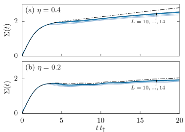
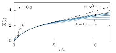
Additionally, Fig. 11 shows the width $\Sigma(t)$ of the density profiles for ${\eta=0.4}$ and ${\eta=0.2}$, as calculated by Eqs. (18) and (22). Compared to the weakly imbalanced case shown in Fig. 6, $\Sigma(t)$ now grows much slower, and Eqs. (18) and (22) are in better agreement, since the distribution is still well concentrated in the center of the chain. For ${\eta=0.2}$, $\Sigma(t)$ appears to remain at a constant plateau up to the maximum time ${t\,t_{\uparrow}=20}$ shown.

Figure 12: (Color online) Spatial width $\Sigma(t)$ for fixed system size $L=14$ and varying imbalances ranging from ${\eta=0}$ to ${\eta=1}$ (arrow) in steps of 0.05. In the balanced case ${\eta=1}$, the width reaches its natural saturation value (dashed line) of ${\Sigma\approx 4}$ [cf. Eq. (26)] rather quickly, while the other curves grow slower as $\eta$ goes to zero. The curve for ${\eta=0}$ remains at around ${\Sigma\approx 2}$.

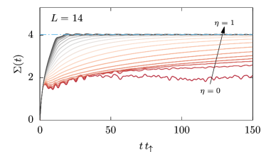
To analyze the $\eta$-dependence of the width in more detail, Fig. 12 shows $\Sigma(t)$ in Eq. (18) on a longer time scale ${t\,t_{\uparrow}\leq 150}$ for various values of $\eta$ and a fixed system size ${L=14}$. While the growth of $\Sigma(t)$ towards the saturation value becomes slower and slower with decreasing $\eta$, we find that even for the smallest value of ${\eta=0.05}$ shown here, $\Sigma(t)$ clearly increases at long times. In contrast, the width in the ${\eta=0}$ case fluctuates around a constant and lower value, which might be interpreted as the Anderson localization length.

IV.3.3 Momentum-space dynamics

Figure 13: (Color online) Discrete Fourier transform $p_{q,\uparrow}(t)$ of the density profile with momentum ${q=2\pi k/L}$ and wave numbers ${k=1,2,3}$ (arrow) for two imbalance ratios (a) ${\eta=0.2}$ and (b) ${\eta=0.1}$ ($L=15$). Another density mode $p_{q,\uparrow}(t)$ (dashed line) for a smaller system size ${L=10}$ with wave number ${k=2}$ is shown for comparison, which has the same momentum ${q=2\pi/5}$ as the mode ${k=3}$ for ${L=15}$.

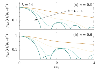
Let us now turn to momentum-space dynamics again. To this end, Figs. 13 (a) and (b) show the discrete Fourier modes $p_{q,\uparrow}(t)$ for imbalance ratios ${\eta=0.2}$ and ${\eta=0.1}$. Note that the data is obtained for an even larger system with ${L=15}$ lattice sites and for momenta ${q=2\pi k/L}$ with ${k=1,2,3}$. Compared to Fig. 7, we find that the $p_{q,\uparrow}(t)$ now decay visibly slower for all wave numbers $k$. Moreover, in contrast to the scaling of decay rates in the case of normal diffusion [cf. Eq. (25)], the density modes now seem to decay at a similar rate for all $k$. Furthermore, even for small ${\eta=0.1}$ and ${k=1}$, we find that $p_{q,\uparrow}(t)$ is clearly non-constant, which suggests that genuine localization is absent for ${\eta>0}$.

To analyze the dependence on system size, Fig. 13 also shows the Fourier mode $p_{q,\uparrow}(t)$ for ${L=10}$ and wave number ${k=2}$. This mode has the same momentum ${q=2\pi/5}$ as the mode ${k=3}$ for ${L=15}$. We find that for both ${\eta=0.2}$ and ${\eta=0.1}$ the decay of $p_{q,\uparrow}(t)$ is almost independent of $L$. Especially for ${\eta=0.1}$, the curves show no significant differences up to the maximum time ${t\,t_{\uparrow}=120}$ shown.

Figure 14: (Color online) (a) Discrete Fourier transform $p_{q,\uparrow}(t)$ of the density profile for fixed momentum ${q=2\pi/14}$ and (b) “lifetime” according to the definition (28) for various distances ${\delta=0.05,\dots,0.5}$ in steps of $0.05$.

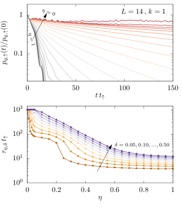
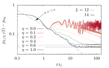
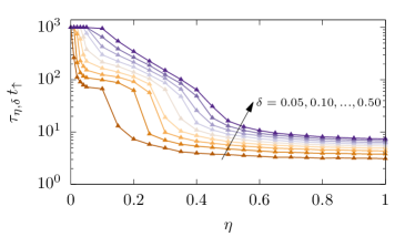
Finally, Fig. 14 (a) shows the relaxation of the Fourier mode $p_{q,\uparrow}(t)$ with the smallest wave number ${k=1}$ for various ${0\leq\eta\leq 1}$. The decay appears to be exponential for ${\eta\gtrsim 0.2}$, albeit very slow for strong imbalances. While for sufficiently small times, all ${\eta>0}$ curves agree with the ${\eta=0}$ curve, they start to deviate at a certain point in time. In order to analyze this separation time from the ${\eta=0}$ curve in more detail, we define

$$\tau_{\eta,\delta}=\max\left\{\ t\ |\ \frac{|\overline{p}_{q,\uparrow}^{\eta}(t)-\overline{p}_{q,\uparrow}^{0}(t)|}{\overline{p}_{q,\uparrow}^{0}(t)}<\delta\ \right\}$$ (28)

using the running averages of the density modes

$$\overline{p}_{q,\uparrow}^{\eta}(t)=\frac{1}{t}\int\limits_{0}^{t}p_{q,\uparrow}^{\eta}(t^{\prime})dt^{\prime}\ .$$ (29)

It measures the maximum time up to which ${\eta=0}$ and ${\eta>0}$ curves do not deviate up to a distance $\delta$. (Note that this maximum time can not exceed the maximum simulation time, here ${t_{\max}\,t_{\uparrow}=1000}$. Moreover, the running averages are used to mitigate the fluctuations of the $p_{q,\uparrow}(t)$, which complicate the extraction of precise separation times.)

The physical picture for this analysis can be understood as follows. For very small but nonzero $\eta$, the heavy particles still appear as a quasi-static disorder potential for the lighter particles, which induces localization analogous to ${\eta=0}$. At some point in time, however, the residual hopping of the heavy particles becomes relevant, which can be seen as an $\eta$-dependent “lifetime” of the Anderson insulator. The corresponding data for different distances $\delta$ is shown in Fig. 14 (b). For every $\delta$, the lifetime grows fast with decreasing $\eta$, but apparently is always finite for all $\eta$ considered. A complementary analysis of $\tau_{\eta,\delta}$, based on the spatial width $\Sigma(t)$ (cf. Fig. 12), can be found in Appendix D and provides a similar picture.

V Conclusion

In this paper, we have studied the real-time dynamics of local charge densities in the Fermi-Hubbard chain with a mass-imbalance between the spin-$\uparrow$ and -$\downarrow$ particles. To this end, we have prepared a certain class of pure states featuring a sharp initial peak of the density profile for the (lighter) spin-$\uparrow$ particles in the middle of the chain and investigated the resulting non-equilibrium dynamics. Relying on dynamical quantum typicality, this dynamics can be related to time-dependent correlation functions at equilibrium.

In the regime of weak and moderate imbalance, ${\eta\gtrsim 0.6}$, we have provided evidence for the emergence of diffusive dynamics, manifesting in (i) Gaussian shape of density profiles, (ii) square-root scaling of the spatial variance in time, and (iii) exponentially decaying modes for small momenta.

In contrast, in the regime of strong imbalance, ${\eta\lesssim 0.6}$, we have observed signatures of anomalous transport, emerging as an exponential rather than a Gaussian shape of density profiles and subdiffusive scaling of spatial variance and density modes in time, consistent with other works Jin et al. (2015); Yao et al. (2016). However, we cannot rule out that this anomalous transport is just a transient effect which crosses over to normal diffusion at even longer times, e.g., at time scales much longer than the “lifetime” of the Anderson insulator.

For very small but nonzero $\eta$, our results are consistent with the absence of genuine localization and support long but finite equilibration times.

Promising future research directions include extensions of the model such as nearest-neighbor interactions and the study of lower temperatures, including potential relations between static and dynamical properties at such temperatures Tezuka and García-García (2012).

Appendix A Typicality relation

To make this paper self-contained, we here derive the typicality relation (12), see also Steinigeweg et al. (2017a). To this end, we start with the correlation function

$$C_{r,\uparrow}(t)=2\braket{(n_{L/2,\uparrow}-p_{\mathrm{eq.}})(n_{r,\uparrow}(t)-p_{\mathrm{eq.}})}+p_{\mathrm{eq.}}$$ (30)

and use ${\braket{n_{r,\uparrow}(t)}=p_{\mathrm{eq.}}=1/2}$, while carrying out the multiplication of the brackets, to obtain

$$C_{r,\uparrow}(t)=2\braket{n_{L/2,\uparrow}n_{r,\uparrow}(t)}=\frac{\mbox{Tr}\left[\,{n_{L/2,\uparrow}n_{r,\uparrow}(t)}\,\right]}{d\,/\,2}\ .$$ (31)

This expression, using cyclic invariance of the trace and the projection property ${n_{L/2,\uparrow}^{2}=n_{L/2,\uparrow}}$, can be written as

$$C_{r,\uparrow}(t) =\frac{\mbox{Tr}\left[\,{n_{L/2,\uparrow}n_{r,\uparrow}(t)n_{L/2,\uparrow}}\,\right]}{d\,/\,2}\ .$$ (32)

Exploiting typicality, the trace can be approximated by a single typical pure state $\ket{\phi}$ as

$$C_{r,\uparrow}(t) =\frac{\bra{\phi}n_{L/2,\uparrow}n_{r,\uparrow}(t)n_{L/2,\uparrow}\ket{\phi}}{\braket{\phi\,}{\,\phi}/\,2}+\epsilon(\ket{\phi})$$ (33)

$$\approx\frac{\left(\bra{\phi}n^{\dagger}_{L/2,\uparrow}\mathrm{e}^{\mathrm{i}Ht}\right)n_{r,\uparrow}\left(\mathrm{e}^{-\mathrm{i}Ht}n^{\phantom{\dagger}}_{L/2,\uparrow}\ket{\phi}\right)}{\braket{\phi\,}{\,\phi}/\,2}\ ,$$

where the the variance of the statistical error $\epsilon(\ket{\phi})$ is bounded from above by ${\text{Var}(\epsilon)(\ket{\phi})<\mathcal{O}(1/d)}$ (at formally infinite temperature) and becomes negligibly small already for intermediate system sizes. With ${\ket{\psi(0)}=n_{L/2,\uparrow}\ket{\phi}/\sqrt{\braket{\phi\,}{\,\phi}/\,2}}$ we arrive at

$$C_{r,\uparrow}(t)\approx\bra{\psi(t)}n_{r,\uparrow}\ket{\psi(t)}=p_{r,\uparrow}(t)$$ (34)

and finally, comparing to (30),

$$p_{r,\uparrow}(t)-p_{\mathrm{eq.}}\approx 2\braket{(n_{L/2,\uparrow}-p_{\mathrm{eq.}})(n_{r,\uparrow}(t)-p_{\mathrm{eq.}})}\ .$$ (35)

Appendix B Equilibration for small $\eta$

Figure 15: (Color online) Decay of the central peak $p_{L/2,\uparrow}(t)$ for ${L=10}$ and long times at ${\eta\leq 0.1}$.

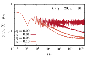
Complementary to Fig. 8, Fig. 15 shows data for the central peak $p_{L/2,\uparrow}(t)$, but now for a smaller system size ${L=10}$ (in the half-filling sector $N_{\uparrow}+N_{\downarrow}=L$) and significantly longer time scales. We find that $p_{L/2,\uparrow}(t)$ ultimately decays towards its equilibrium value, even for very small values of $\eta$. Note that the interaction strength in Fig. 15 is chosen as ${U/t_{\uparrow}=20}$, analogous to earlier investigations in Ref. Yao et al. (2016), where similar findings were presented for momentum-space observables.

Appendix C L-independence of density profiles

Figure 16: (Color online) Comparison of density profiles for two system sizes ${L=13,14}$ and a few exemplary imbalance ratios $\eta$. The overall behavior coincides nicely for both $L$, apart from slight deviations at the boundaries.

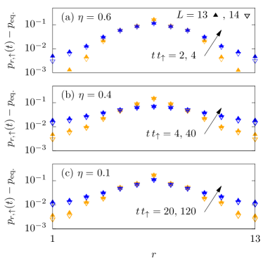
To demonstrate the $L$-independence for the scaling of the density profiles, Fig. 16 shows $p_{r,\uparrow}(t)$ for two system sizes with ${L=13}$ and $14$ and exemplary values for times $t$ and imbalances $\eta$. Apart from small deviations at the tails, we find that the profiles for different $L$ are in very good agreement. This fact also demonstrates the accuracy of the typicality approach.

Appendix D Anderson lifetime

Figure 17: (Color online) “Lifetime” in analogy to the definition (28) for various distances ${\delta=0.05,\dots,0.5}$ in steps of $0.05$, now based on the spatial width $\Sigma(t)$ shown in Fig. 12.

In addition to Fig. 14 (b), Fig. 17 shows another analysis of the lifetime $\tau_{\eta,\delta}$. Here, $\tau_{\eta,\delta}$ is calculated in analogy to (28), but based on the spatial width $\Sigma(t)$ (cf. Fig. 12),

$$\tau_{\eta,\delta}=\max\left\{\ t\ |\ \frac{|\overline{\Sigma}^{\eta}(t)-\overline{\Sigma}^{0}(t)|}{\overline{\Sigma}^{0}(t)}<\delta\ \right\}$$ (36)

with

$$\overline{\Sigma}^{\eta}(t)=\frac{1}{t}\int\limits_{0}^{t}\Sigma^{\eta}(t^{\prime})dt^{\prime}\ .$$ (37)

In comparison to Fig. 14 (b), Fig. 17 provides a very similar picture for the $\eta$-dependent lifetime.

References

- Bloch et al. (2012) I. Bloch, J. Dalibard, and S. Nascimbène, Nat. Phys. 8, 267 (2012).
- Blatt and Roos (2012) R. Blatt and C. F. Roos, Nat. Phys. 8, 277 (2012).
- Polkovnikov et al. (2011) A. Polkovnikov, K. Sengupta, A. Silva, and M. Vengalattore, Rev. Mod. Phys. 83, 863 (2011).
- Eisert et al. (2015) J. Eisert, M. Friesdorf, and C. Gogolin, Nat. Phys. 11, 124 (2015).
- D’Alessio et al. (2016) L. D’Alessio, Y. Kafri, A. Polkovnikov, and M. Rigol, Adv. Phys. 65, 239 (2016).
- Gogolin and Eisert (2016) C. Gogolin and J. Eisert, Rep. Prog. Phys. 79, 056001 (2016).
- Borgonovi et al. (2016) F. Borgonovi, F. Izrailev, L. F. Santos, and V. Zelevinsky, Phys. Rep. 626, 1 (2016).
- Deutsch (1991) J. M. Deutsch, Phys. Rev. A 43, 2046 (1991).
- Srednicki (1994) M. Srednicki, Phys. Rev. E 50, 888 (1994).
- Rigol et al. (2008) M. Rigol, V. Dunjko, and M. Olshanii, Nature 452, 854 (2008).
- Anderson (1958) P. W. Anderson, Phys. Rev. 109, 1492 (1958).
- Abrahams et al. (1979) E. Abrahams, P. W. Anderson, D. C. Licciardello, and T. V. Ramakrishnan, Phys. Rev. Lett. 42, 673 (1979).
- Roati et al. (2008) G. Roati, C. D’Errico, L. Fallani, M. Fattori, C. Fort, M. Zaccanti, G. Modugno, M. Modugno, and M. Inguscio, Nature 453, 895 (2008).
- Billy et al. (2008) J. Billy, V. Josse, Z. Zuo, A. Bernard, B. Hambrecht, P. Lugan, D. Clément, L. Sanchez-Palencia, P. Bouyer, and A. Aspect, Nature 453, 891 (2008).
- Nandkishore and Huse (2015) R. Nandkishore and D. A. Huse, Annu. Rev. Condens. Matter Phys. 6, 15 (2015).
- Abanin et al. (2019) D. A. Abanin, E. Altman, I. Bloch, and M. Serbyn, Rev. Mod. Phys. 91, 021001 (2019).
- Schreiber et al. (2015) M. Schreiber, S. S. Hodgman, P. Bordia, H. P. Luschen, M. H. Fischer, R. Vosk, E. Altman, U. Schneider, and I. Bloch, Science 349, 842 (2015).
- Gopalakrishnan and Parameswaran (2020) S. Gopalakrishnan and S. Parameswaran, Phys. Rep. 862, 1 (2020).
- Lüschen et al. (2017) H. P. Lüschen, P. Bordia, S. S. Hodgman, M. Schreiber, S. Sarkar, A. J. Daley, M. H. Fischer, E. Altman, I. Bloch, and U. Schneider, Phys. Rev. X 7, 011034 (2017).
- Smith et al. (2016) J. Smith, A. Lee, P. Richerme, B. Neyenhuis, P. W. Hess, P. Hauke, M. Heyl, D. A. Huse, and C. Monroe, Nat. Phys. 12, 907 (2016).
- Richter et al. (2019) J. Richter, N. Casper, W. Brenig, and R. Steinigeweg, Phys. Rev. B 100, 144423 (2019).
- Richter et al. (2020) J. Richter, D. Schubert, and R. Steinigeweg, Phys. Rev. Research 2, 013130 (2020).
- Prelovšek et al. (2016) P. Prelovšek, O. S. Barišić, and M. Žnidarič, Phys. Rev. B 94, 241104(R) (2016).
- Kozarzewski et al. (2018) M. Kozarzewski, P. Prelovšek, and M. Mierzejewski, Phys. Rev. Lett. 120, 246602 (2018).
- Carleo et al. (2012) G. Carleo, F. Becca, M. Schiró, and M. Fabrizio, Sci. Rep. 2, 243 (2012).
- De Roeck and Huveneers (2014a) W. De Roeck and F. Huveneers, Phys. Rev. B 90, 165137 (2014a).
- De Roeck and Huveneers (2014b) W. De Roeck and F. Huveneers, Commun. Math. Phys. 332, 1017 (2014b).
- De Roeck and Huveneers (2015) W. De Roeck and F. Huveneers, “Can Translation Invariant Systems Exhibit a Many-Body Localized Phase?” in From Particle Systems to Partial Differential Equations II, edited by P. Gonçalves and A. J. Soares (Springer International Publishing, Cham, 2015) pp. 173–192.
- Grover and Fisher (2014) T. Grover and M. P. A. Fisher, J. Stat. Mech. 2014, P10010 (2014).
- Schiulaz and Müller (2014) M. Schiulaz and M. Müller, in AIP Conf. Proc., Vol. 1610 (2014) pp. 11–23.
- Altman and Vosk (2015) E. Altman and R. Vosk, Annu. Rev. Condens. Matter Phys. 6, 383 (2015).
- Papić et al. (2015) Z. Papić, E. M. Stoudenmire, and D. A. Abanin, Ann. Phys. (NY) 362, 714 (2015).
- Schiulaz et al. (2015) M. Schiulaz, A. Silva, and M. Müller, Phys. Rev. B 91, 184202 (2015).
- Hickey et al. (2016) J. M. Hickey, S. Genway, and J. P. Garrahan, J. Stat. Mech. 2016, 054047 (2016).
- Yao et al. (2016) N. Y. Yao, C. R. Laumann, J. I. Cirac, M. D. Lukin, and J. E. Moore, Phys. Rev. Lett. 117, 240601 (2016).
- Smith et al. (2017) A. Smith, J. Knolle, D. L. Kovrizhin, and R. Moessner, Phys. Rev. Lett. 118, 266601 (2017).
- Michailidis et al. (2018) A. A. Michailidis, M. Žnidarič, M. Medvedyeva, D. A. Abanin, T. Prosen, and Z. Papić, Phys. Rev. B 97, 104307 (2018).
- Brenes et al. (2018) M. Brenes, M. Dalmonte, M. Heyl, and A. Scardicchio, Phys. Rev. Lett. 120, 030601 (2018).
- Sirker (2019) J. Sirker, Phys. Rev. B 99, 075162 (2019).
- Gamayun et al. (2014) O. Gamayun, O. Lychkovskiy, and V. Cheianov, Phys. Rev. E 90, 032132 (2014).
- Jin et al. (2015) F. Jin, R. Steinigeweg, F. Heidrich-Meisner, K. Michielsen, and H. De Raedt, Phys. Rev. B 92, 205103 (2015).
- Prosen and Žnidarič (2012) T. Prosen and M. Žnidarič, Phys. Rev. B 86, 125118 (2012).
- Karrasch et al. (2017) C. Karrasch, T. Prosen, and F. Heidrich-Meisner, Phys. Rev. B 95, 060406(R) (2017).
- Steinigeweg et al. (2017a) R. Steinigeweg, F. Jin, H. De Raedt, K. Michielsen, and J. Gemmer, Phys. Rev. E 96, 020105(R) (2017a).
- Ilievski et al. (2018) E. Ilievski, J. De Nardis, M. Medenjak, and T. Prosen, Phys. Rev. Lett. 121, 230602 (2018).
- Paredes et al. (2005) B. Paredes, F. Verstraete, and J. I. Cirac, Phys. Rev. Lett. 95, 140501 (2005).
- Andraschko et al. (2014) F. Andraschko, T. Enss, and J. Sirker, Phys. Rev. Lett. 113, 217201 (2014).
- Zhao et al. (2016) Y. Zhao, F. Andraschko, and J. Sirker, Phys. Rev. B 93, 205146 (2016).
- Enss et al. (2017) T. Enss, F. Andraschko, and J. Sirker, Phys. Rev. B 95, 045121 (2017).
- Essler et al. (2005) F. H. L. Essler, H. Frahm, F. Göhmann, A. Klümper, and V. E. Korepin, The One-Dimensional Hubbard Model (Cambridge University Press, 2005).
- Falicov and Kimball (1969) L. M. Falicov and J. C. Kimball, Phys. Rev. Lett. 22, 997 (1969).
- Lyżwa and Domański (1994) R. Lyżwa and Z. Domański, Phys. Rev. B 50, 11381 (1994).
- Bartsch and Gemmer (2009) C. Bartsch and J. Gemmer, Phys. Rev. Lett. 102, 110403 (2009).
- Bartsch and Gemmer (2011) C. Bartsch and J. Gemmer, EPL (Europhys. Lett.) 96, 60008 (2011).
- Steinigeweg et al. (2017b) R. Steinigeweg, F. Jin, D. Schmidtke, H. De Raedt, K. Michielsen, and J. Gemmer, Phys. Rev. B 95, 035155 (2017b).
- Schnack et al. (2020a) J. Schnack, J. Richter, and R. Steinigeweg, Phys. Rev. Research 2, 013186 (2020a).
- Schnack et al. (2020b) J. Schnack, J. Richter, T. Heitmann, J. Richter, and R. Steinigeweg, Z. Naturforsch. A 75, 465 (2020b).
- Heitmann et al. (2020) T. Heitmann, J. Richter, D. Schubert, and R. Steinigeweg, Z. Naturforsch. A 75, 421 (2020).
- Gemmer and Mahler (2003) J. Gemmer and G. Mahler, Eur. Phys. J. B 31, 249 (2003).
- Iitaka and Ebisuzaki (2003) T. Iitaka and T. Ebisuzaki, Phys. Rev. Lett. 90, 047203 (2003).
- Iitaka and Ebisuzaki (2004) T. Iitaka and T. Ebisuzaki, Phys. Rev. E 69, 057701 (2004).
- Goldstein et al. (2006) S. Goldstein, J. L. Lebowitz, R. Tumulka, and N. Zanghì, Phys. Rev. Lett. 96, 050403 (2006).
- Popescu et al. (2006) S. Popescu, A. J. Short, and A. Winter, Nat. Phys. 2, 754 (2006).
- Reimann (2007) P. Reimann, Phys. Rev. Lett. 99, 160404 (2007).
- White (2009) S. R. White, Phys. Rev. Lett. 102, 190601 (2009).
- Sugiura and Shimizu (2012) S. Sugiura and A. Shimizu, Phys. Rev. Lett. 108, 240401 (2012).
- Sugiura and Shimizu (2013) S. Sugiura and A. Shimizu, Phys. Rev. Lett. 111, 010401 (2013).
- Elsayed and Fine (2013) T. A. Elsayed and B. V. Fine, Phys. Rev. Lett. 110, 070404 (2013).
- Steinigeweg et al. (2014a) R. Steinigeweg, J. Gemmer, and W. Brenig, Phys. Rev. Lett. 112, 120601 (2014a).
- Steinigeweg et al. (2014b) R. Steinigeweg, A. Khodja, H. Niemeyer, C. Gogolin, and J. Gemmer, Phys. Rev. Lett. 112, 130403 (2014b).
- Monnai and Sugita (2014) T. Monnai and A. Sugita, J. Phys. Soc. Jpn. 83, 094001 (2014).
- Reimann (2016) P. Reimann, Nat. Commun. 7, 10821 (2016).
- Reimann (2018) P. Reimann, Phys. Rev. E 97, 062129 (2018).
- de Vries and De Raedt (1993) P. de Vries and H. De Raedt, Phys. Rev. B 47, 7929 (1993).
- De Raedt and Michielsen (2006) H. De Raedt and K. Michielsen, “Computational Methods for Simulating Quantum Computers,” in Handbook of Theoretical and Computational Nanotechnology, Vol. 3, edited by M. Rieth and W. Schommers (American Scientific Publishers, Los Angeles, 2006) Chap. 1, p. 248.
- Tal‐Ezer and Kosloff (1984) H. Tal‐Ezer and R. Kosloff, J. Chem. Phys. 81, 3967 (1984).
- Dobrovitski and De Raedt (2003) V. V. Dobrovitski and H. A. De Raedt, Phys. Rev. E 67, 056702 (2003).
- Weiße et al. (2006) A. Weiße, G. Wellein, A. Alvermann, and H. Fehske, Rev. Mod. Phys. 78, 275 (2006).
- Nauts and Wyatt (1983) A. Nauts and R. E. Wyatt, Phys. Rev. Lett. 51, 2238 (1983).
- Heitmann and Schnack (2019) T. Heitmann and J. Schnack, Phys. Rev. B 99, 134405 (2019).
- (81) B. Bertini, F. Heidrich-Meisner, C. Karrasch, T. Prosen, R. Steinigeweg, and M. Žnidarič, arXiv:2003.03334 .
- Steinigeweg et al. (2009) R. Steinigeweg, H. Wichterich, and J. Gemmer, EPL (Europhys. Lett.) 88, 10004 (2009).
- Yan et al. (2015) Y. Yan, F. Jiang, and H. Zhao, Eur. Phys. J. B 88, 11 (2015).
- Žnidarič et al. (2016) M. Žnidarič, A. Scardicchio, and V. K. Varma, Phys. Rev. Lett. 117, 040601 (2016).
- Tezuka and García-García (2012) M. Tezuka and A. M. García-García, Phys. Rev. A 85, 031602(R) (2012).