Baseline Estimation of Commercial Building HVAC Fan Power Using Tensor Completion

Abstract

Commercial building heating, ventilation, and air conditioning (HVAC) systems have been studied for providing ancillary services to power grids via demand response (DR). One critical issue is to estimate the counterfactual baseline power consumption that would have prevailed without DR. Baseline methods have been developed based on whole building electric load profiles. New methods are necessary to estimate the baseline power consumption of HVAC sub-components (e.g., supply and return fans), which have different characteristics compared to that of the whole building. Tensor completion can estimate the unobserved entries of multi-dimensional tensors describing complex data sets. It exploits high-dimensional data to capture granular insights into the problem. This paper proposes to use it for baselining HVAC fan power, by utilizing its capability of capturing dominant fan power patterns. The tensor completion method is evaluated using HVAC fan power data from several buildings at the University of Michigan, and compared with several existing methods. The tensor completion method generally outperforms the benchmarks.

This work was supported in part by the U.S. Department of Energy via the project IDREEM: Impact of Demand Response on short and long term building Energy Efficiency Metrics funded by the Building Technologies Office under contract number DE-AC02-76SF00515. Hong was supported in part by the NSF BIGDATA grant IIS 1837992 and the Dean’s Fund for Postdoctoral Research of the Wharton School.

I Introduction

Demand response (DR) is a strategy that incentivizes changes in building electricity consumption to improve grid reliability and economics. Owing to the large thermal inertia of commercial buildings, their heating, ventilation, and air conditioning (HVAC) systems can provide ancillary services to electric power systems through DR while respecting the occupants’ comfort. For example, in [1], the power consumption of HVAC system fans is controlled to track a regulation signal.

A critical challenge in implementing DR is to estimate the power consumption that would have prevailed without the DR event, referred to as the baseline, which is needed for financial settlement and DR impact analysis. Therefore, a variety of baseline estimation methods have been developed, generally based on whole building electric load profiles. Now, with increasing availability of submetering in commercial buildings, it is anticipated that those more granular data can be utilized to attain more accurate baseline estimates and more granular insights into the responsive components, e.g., fans in the HVAC systems. To this end, new baseline methods are needed, as the existing methods do not always work well with the new types of data.

Baseline methods in the literature can be classified into three categories, i.e., averaging, regression, and control group methods. They are generally used to baseline whole building electric load. Averaging methods use the average load of selected recent days without DR events to estimate the baseline. They are easy to implement, but typically have large errors [2]. Regression methods fit a linear or non-linear function to describe the relationship between the load and explanatory variables such as outdoor temperature, and then use it to estimate the baseline. However, their applicability to baseline HVAC fan power is limited, e.g., due to the weak correlation between HVAC fan power and outdoor temperature [3]. Control group methods identify and utilize the data of similar customers to estimate the baseline. Normally, a large data set is required [4].

In [1], signal bandwidth separation is used to estimate the baseline fan power, since the baseline fan power has a much lower bandwidth than the DR signal (a frequency regulation signal). However, this approach is only applicable when the DR signal is of a high frequency. In [5] [6], a linear interpolation method is used to baseline fan power. It uses least squares to fit a linear baseline to the fan power data over the 5-minute period just before the DR event and the 5-minute period after a settling window (i.e., the period during which the fans settle back to their normal operation). However, it does not perform consistently well, generating large errors in some cases.

This paper proposes an approach based on tensor decomposition. Tensor decomposition is an unsupervised data analysis method that can find dominant patterns across multiple dimensions, e.g., time, fan, and day, in the case of submetered fan power data. See [7] for a survey. It has numerous applications, from cybersecurity [8] to energy breakdown [9] to power system model reduction [10], and was specifically applied to submetered fan power data in our preliminary work [11], where it captured dominant load patterns in the HVAC supply and return fans.

Tensor completion is the closely related problem of imputing missing or unobserved entries of a tensor. The ubiquity of tensor structure makes it a fundamental problem with broad interest and highly active research; see [12] for a recent survey. This paper considers tensor completion via generalized canonical polyadic (GCP) tensor decomposition [13]. GCP tensor decomposition allows for fitting only observed tensor entries, making it suitable for tensor completion, and it has the added ability to do outlier-robust fitting via an appropriate choice of fitting loss function. Other tensor completion approaches could be of interest, though we leave further exploration for future work.

This work proposes using GCP tensor completion to estimate HVAC fan power baselines by considering fan power data within the DR event windows to be missing. Specifically, we estimate baseline fan power during DR events from a low-rank GCP tensor approximation of fan power measurements outside the DR events. Doing so encourages baseline estimates to have load patterns that are consistent among different fans and different days. The tensor completion method is evaluated with power consumption data of HVAC system supply fans and return fans that are submetered in three buildings at the University of Michigan, i.e., Bob and Betty Beyster Building (BBB), Rackham Graduate School (RAC) and Weill Hall (WH).

The contributions of this work are threefold: 1) A new method for baselining HVAC fan power is developed based on tensor completion; 2) The impact of data granularity (i.e., time intervals, aggregation levels) on the method is investigated; and 3) The tensor completion method is compared with the three best methods among the ones tested in our previous work [3] using real-world data. Section II provides a brief problem statement. Section III introduces the tensor completion method. Section IV presents case studies. Section V concludes the paper and discusses the future work.

II Problem Statement

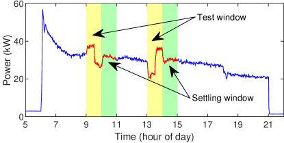
Figure 1: Total fan power trace of RAC on an event day (Sep. 26, 2017).

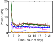
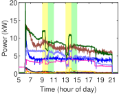
Figure 2: Per-fan power traces of RAC on a baseline day (Left, Sep. 5, 2017) and an event day (Right, Sep. 26, 2017). One-minute interval data are shown.

Fig. 1 shows two DR tests on RAC. The morning event is called an up-down test. During the test window (9-10am), room temperature setpoints are decreased below nominal values for 30 minutes and then increased symmetrically above nominal values for 30 minutes, causing HVAC fan power to go up and then go down. The fans return to their normal operation after a settling window, which we assume to be one hour. The afternoon event is a down-up test with opposite room temperature setpoint changes. These tests are designed to assess the energy efficiency of fast DR actions, which primarily impact the fans [14]. To this end, we need to estimate the fan power that would have prevailed without DR events, i.e., the baseline fan power during each event window (including the test window and settling window). In our case study we differentiate between the morning event window (9-11am) and the afternoon event window (1-3pm).

A commercial building HVAC system normally has multiple supply fans and return fans. Our submetering equipment provides us with 1-minute resolution power data from each fan. That is, while our task is baselining the total fan power, we have data of a higher granularity, i.e., the power consumption of each fan. Fig. 2 (Right) shows the power trace of each fan in RAC on the same test day as used in Fig. 1, while Fig. 2 (Left) shows fan power traces on a day without DR events, i.e., a baseline day. Data from baseline days corresponds to normal operation of HVAC fans without DR events, and thus can be used to estimate the baseline fan power on DR event days.

Specifically, our baseline estimation problem can be described as follows: Given the power profile of each fan in time slots outside event window(s) on days with DR event(s) and the power profile of each fan on baseline days, estimate the total fan power that would have prevailed in time slots within event window(s) on event days if DR event(s) did not happen. Other baseline methods may have different data requirements; the above problem description is for our tensor completion method.

TABLE I: Summary of Data Sets

	# of fans (SF: supply fan; RF: return fan.)	# of baseline days	Total fan power in day mode (kW)
			Peak	Average
BBB-2017	1 SF, 1 RF	55 (in Jun.-Oct.)	35.8	12.2
BBB-2018	4 SFs, 3 RFs	16 (in Oct.)	105.3	38.3
RAC-2017	4 SFs, 4 RFs	49 (in Jul.-Oct.)	63.6	18.7
RAC-2018	4 SFs, 4 RFs	30 (in May-Oct.)	63.0	24.7
WH-2017	2 SFs, 2 RFs	86 (in Jun.-Oct.)	125.9	45.7

We evaluate the accuracy of the proposed baseline estimation method using data from baseline days in a data set. As no DR events happen on a baseline day, the measured total fan power is the true baseline during event windows (without tests) for the same baseline day. The errors of the proposed baseline estimation method can be assessed by comparing the estimates with the measurements. Table I lists the five data sets used in this work, corresponding to five different building-years. To estimate the baseline in event window(s) on a given day of a building-year, only data from the same building-year is used.

III Proposed Tensor Completion Method

Motivated by [11], which uses the canonical polyadic (CP) tensor decomposition to capture dominant fan power behavior, we investigate using tensor completion to form baseline estimates. As shown in Fig. 3, we form the fan power data into a three-way time $\times$ fan $\times$ day tensor, i.e., a three-dimensional $T\times N\times S$ array $\boldsymbol{\mathscr{P}}\in\mathbb{R}^{T\times N\times S}$ whose $(i,j,k)$th entry $p_{ijk}$ is the power at time slot $i$ of fan $j$ on day $k$, with $i=1,2,...,T$, $j=1,2,...,N$ and $k=1,2,...,S$. Using this representation, correlations across fans and days become naturally expressed as patterns across each of the three modes (time, fan, and day), and can be captured by tensor decomposition.

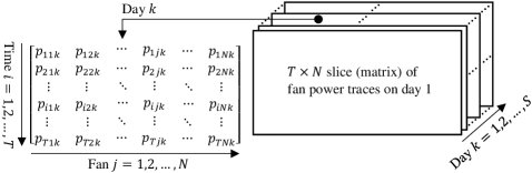
Figure 3: Formation of a three-way tensor $\boldsymbol{\mathscr{P}}$ based on HVAC fan power data.

In the proposed method, we include data from $S-1$ baseline days and $1$ event day in $\boldsymbol{\mathscr{P}}$. We consider the to-be-estimated baseline power within DR event window(s) of the event day as missing or unobserved measurements, and impute these tensor entries by approximating the remaining (known) entries with a low-rank tensor $\boldsymbol{\widehat{\mathscr{P}}}$ as shown in Fig. 4. Namely, we estimate the counterfactual measurements by the entries of $\boldsymbol{\widehat{\mathscr{P}}}$, where $\boldsymbol{\widehat{\mathscr{P}}}$ is rank (at most) $r$. As illustrated in Fig. 4, $\boldsymbol{\widehat{\mathscr{P}}}$ is a sum of $r$ outer products:

$$\boldsymbol{\widehat{\mathscr{P}}}=\ell^{(1)}\circ\omega^{(1)}\circ\bar{\omega}^{(1)}+\cdots+\ell^{(r)}\circ\omega^{(r)}\circ\bar{\omega}^{(r)}.$$ (1)

where $\circ$ denotes an outer product, as shown in Fig. 4. Namely, the entries of $\boldsymbol{\widehat{\mathscr{P}}}$ are:

$$\widehat{p}_{ijk}=\ell^{(1)}_{i}\omega^{(1)}_{j}\bar{\omega}^{(1)}_{k}+\cdots+\ell^{(r)}_{i}\omega^{(r)}_{j}\bar{\omega}^{(r)}_{k}.$$ (2)

The $(i,j,k)$th entry $\widehat{p}_{ijk}$ of $\boldsymbol{\widehat{\mathscr{P}}}$ is the approximated power at time slot $i$ of fan $j$ on day $k$. The vectors forming $\boldsymbol{\widehat{\mathscr{P}}}$ capture dominant underlying patterns across each mode: $\ell^{(1)},...,\ell^{(r)}\in\mathbb{R}^{T}$ are factors along the time mode, $\omega^{(1)},...,\omega^{(r)}\in\mathbb{R}^{N}$ are factors along the fan mode, and $\bar{\omega}^{(1)},...,\bar{\omega}^{(r)}\in\mathbb{R}^{S}$ are factors along the day mode.

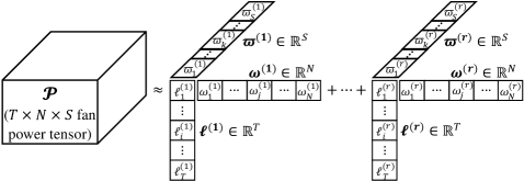
Figure 4: Rank-$r$ tensor decomposition of the fan power tensor. The left-hand side of the approximation is the fan power tensor $\boldsymbol{\mathscr{P}}$. The right-hand side is a sum of $r$ outer products, referred to as $\boldsymbol{\widehat{\mathscr{P}}}$. (Time slot index $i=1,2,...,T$; fan index $j=1,2,...,N$; and day index $k=1,2,...,S$.)

We obtain $\boldsymbol{\widehat{\mathscr{P}}}$ via the GCP tensor decomposition [13] of $\boldsymbol{\mathscr{P}}$ that minimizes the following loss function:

$$F(\boldsymbol{\widehat{\mathscr{P}}},\boldsymbol{\mathscr{P}})\coloneqq\sum_{(i,j,k)\in\boldsymbol{\Omega}}f(\widehat{p}_{ijk},p_{ijk}),\quad\text{s.t. }\operatorname{rank}\boldsymbol{\widehat{\mathscr{P}}}\leq r.$$ (3)

where the sum is over indices $(i,j,k)\in\boldsymbol{\Omega}$ which are known, i.e., not to be estimated. Namely, indices $(i,j,k)$ in the set $\boldsymbol{\Omega}$ include: a) all entries from baseline days, and b) all entries outside the DR event window(s) from event days. A commonly-used loss function is the $L_{2}$-norm loss function, i.e., the squared error loss function. For a given $(i,j,k)\in\boldsymbol{\Omega}$, this loss is calculated by:

$$g(\widehat{p}_{ijk},p_{ijk})\coloneqq\left(\widehat{p}_{ijk}-p_{ijk}\right)^{2}.$$ (4)

In this work, we use the Huber loss function instead [15]:

$$f(\widehat{p}_{ijk},p_{ijk};\Delta)\coloneqq\begin{cases}g(\widehat{p}_{ijk},p_{ijk}),\,\,\text{if }|\widehat{p}_{ijk}-p_{ijk}|\leq\Delta;\\ 2\Delta|\widehat{p}_{ijk}-p_{ijk}|-\Delta^{2},\,\,\,\,\,\text{otherwise}.\end{cases}$$ (5)

Fig. 5 compares this loss function ($\Delta=0.25$) with the usual squared error loss of conventional CP tensor decomposition. The Huber loss penalizes the square of small residuals between $\boldsymbol{\widehat{\mathscr{P}}}$ and $\boldsymbol{\mathscr{P}}$, encouraging a conventional least-squares fit of $\boldsymbol{\widehat{\mathscr{P}}}$ to $\boldsymbol{\mathscr{P}}$, but penalizes large residuals, i.e., potential outliers, by only their magnitudes. Doing so can make the results more robust to outliers in the data [16]. In our experiments, we find that using the Huber loss function attains much smaller baseline errors than using the squared error function for data sets BBB-2018 and WH-2017, which have easily identifiable outliers.

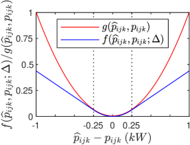
Figure 5: Huber loss function ($f$) with $\Delta=0.25$ and $L_{2}$-norm loss function ($g$).

To summarize, we propose to: 1) approximate the known measurements in the fan power tensor $\boldsymbol{\mathscr{P}}$ with a rank-$r$ tensor $\boldsymbol{\widehat{\mathscr{P}}}$ by GCP tensor decomposition; then 2) estimate counterfactual measurements using the entries of $\boldsymbol{\widehat{\mathscr{P}}}$. This approach estimates baselines by encouraging a low-rank tensor structure and is a tensor generalization of the low-rank matrix completion. Tensor decomposition serves as a tensor analogue to Principal Component Analysis (PCA), where the factors in 1 correspond to principal components. The generalization enables this tensor approach to exploit correlation along time, fan, and day.

III-A Optimization Algorithm for GCP Tensor Decomposition

We use the implementation of GCP tensor decomposition in the MATLAB Tensor Toolbox [17] that minimizes 3 with respect to the factors $\ell^{(1)},...,\ell^{(r)}\in\mathbb{R}^{T}$, $\omega^{(1)},...,\omega^{(r)}\in\mathbb{R}^{N}$, and $\bar{\omega}^{(1)},...,\bar{\omega}^{(r)}\in\mathbb{R}^{S}$ of $\boldsymbol{\widehat{\mathscr{P}}}$ as defined in 1. The toolbox function gcp_opt minimizes this non-convex optimization problem via a first-order algorithm, i.e., the limited-memory BFGS with bound constraints (L-BFGS-B) algorithm [18], using the special form of the gradient [13, Section 4.1]. Further details are available in [13]. This approach is not guaranteed to always find a global minimum, so we run four trials with different initializations and select the best trial, i.e., the trial with the smallest final objective function value.

III-B Selecting a Rank

The proposed approach requires that we choose the approximation rank $r$. Using a rank that is too large can underconstrain $\boldsymbol{\widehat{\mathscr{P}}}$. For example, for any $\boldsymbol{\widehat{\mathscr{P}}}\in\mathbb{R}^{T\times N\times S}$ [19]:

$$\operatorname{rank}\boldsymbol{\widehat{\mathscr{P}}}\leq\min(TN,TS,NS).$$ (6)

Thus, for $r=\min(TN,TS,NS)$, any tensor $\boldsymbol{\widehat{\mathscr{P}}}$ matching $\boldsymbol{\mathscr{P}}$ on the known entries minimizes 3 regardless of how it estimates counterfactual baselines, making the estimates arbitrary. On the other hand, a rank that is too small can insufficiently capture the diversity of fan power behavior, forming baseline estimates from only broad coarse-grain fan power patterns. Hence, there is a trade-off between data overfit that is incurred at large ranks and approximation error that is incurred at small ranks. This trade-off is affected both by how low-rank baseline fan power behavior is, which is unknown, and by how much of the tensor needs to be estimated, making optimal rank selection challenging.

Fitting higher rank approximations to the data can also take more time, and in our preliminary experiments, a rank of 12 seemed to reasonably balance these various trade-offs. Using higher rank approximations increased computation time without yielding large performance improvements. Thus, we use a rank of 12 for the tensor completions in this paper. Developing systematic approaches to rank selection for baseline estimation is important future work.

III-C Data Granularity

As mentioned, the data we obtain from the submeters is 1-minute resolution power data for each HVAC fan. As reported in [20] [21], the performance of an electric load forecasting method can be impacted by the data temporal and spatial granularity. Therefore, we investigate the impact of data granularity on the performance of our method. We test our method using 1-minute, 5-minute, 15-minute and 30-minute interval data. We select 5-minute, 15-minute and 30-minute intervals because these are frequently used in the electric load forecasting and prediction literature [4] [21]-[22]. We do not test the method using data of longer intervals, as we are interested in baselining fan power at subhourly timescales corresponding to our DR experiments. In this work, the 5-minute data are obtained by averaging the original 1-minute data for every 5 minutes, and likewise for the 15-minute and 30-minute data sets. In [11], HVAC fan power patterns are investigated with per-fan power data and total fan power data, respectively. We also test our method using per-fan power data versus total fan power data in this work. In the latter case, although the fan power tensor’s dimension becomes $T\times S$, the tensor completion method is still applicable.

III-D Performance Metrics

Three metrics are used to evaluate the proposed baseline method’s performance. Let $p_{i}$ and $\widehat{p}_{i}$ be the measured and estimated total fan power at time slot $i$, respectively. Also let $\boldsymbol{\tau}=\{\tau_{s},\tau_{s+1},...,\tau_{e}\}$ be the time slots within an event window. The first metric is the coefficient of variation (CV), which is also referred to as the coefficient of variance of root mean squared error (CV-RMSE). It measures the baseline accuracy using the ratio of the standard deviation of estimation errors to the mean of the true values. For each event window CV can be calculated by [23]:

$$CV(\%)=\frac{\sqrt{\frac{1}{\left|\boldsymbol{\tau}\right|-1}\sum_{i=\tau_{s}}^{\tau_{e}}\left(\widehat{p}_{i}-p_{i}\right)^{2}}}{\frac{1}{\left|\boldsymbol{\tau}\right|}\sum_{i=\tau_{s}}^{\tau_{e}}p_{i}}\times 100.$$ (7)

Namely, CV is the RMSE normalized by the true mean value.

The second metric is the normalized mean bias error (NMBE). Positive and negative values indicate overestimation and underestimation of the baseline, respectively. For each event window NMBE can be calculated by [23]:

$$NMBE(\%)=\frac{\frac{1}{\left|\boldsymbol{\tau}\right|-1}\sum_{i=\tau_{s}}^{\tau_{e}}\left(\widehat{p}_{i}-p_{i}\right)}{\frac{1}{\left|\boldsymbol{\tau}\right|}\sum_{i=\tau_{s}}^{\tau_{e}}p_{i}}\times 100.$$ (8)

CV and NMBE are recommended by the American Society of Heating, Refrigeration and Air Conditioning Engineers (ASHRAE) and are commonly adopted in electric load forecasting or prediction studies [20] [21] [24]. ASHRAE also prescribes the acceptable tolerances for those two metrics [23].

The third metric is the additional energy consumption (AEC), which compares the energy consumption during an event window of an event day with the baseline [6]. While it was designed to assess energy efficiency, it can also be used to assess baseline method performance because the AEC will be zero if the baseline method is perfectly unbiased. Let $\delta$ indicate the data temporal resolution in minutes. For example, for 15-minute interval data, $\delta=15$. For each event window AEC can be calculated by:

$$AEC(\mathrm{kWh})=\sum_{i=\tau_{s}}^{\tau_{e}}\left(\widehat{p}_{i}-p_{i}\right)\times\frac{\delta}{60}.$$ (9)

Note that AEC is similar to NMBE without normalization. It is a metric to measure the bias of baseline methods. It is used here to provide more straightforward assessment of baseline errors in terms of energy consumption.

For each data set, leave-one-out cross-validation [25] is conducted to attain metric statistics. Specifically, the baseline fan power within event windows on a given baseline day $k$ is assumed unknown and estimated based on all other entries of $\boldsymbol{\mathscr{P}}$. The estimate is compared with the true baseline to calculate metric values. This process is repeated for each baseline day $k=1,2,...,S$. Metric statistics thus are obtained based on the values of each metric for each event window on different days.

IV Case Studies

In this section, we apply the proposed baseline method and benchmark methods to the data sets listed in Table I. As described in Section II, the baseline methods are evaluated using data from baseline days. Since no DR events happen on baseline days, the measured actual total fan power is the true baseline. Errors of a baseline method can be assessed by comparing its baseline estimates with the true baselines (i.e., the measurements).

IV-A Impact of Temporal Frequency of the Data

TABLE II: Mean values and Standard Deviations ($\sigma$) of CV and NMBE for Different Temporal Frequencies of the Data

		1-min	5-min	15-min	30-min
CV (%), 9-11am: mean ($\sigma$)	BBB-2017	15.63 (1.93)	8.16 (1.97)	6.12 (1.79)	6.12 (2.49)
	BBB-2018	10.01 (2.21)	5.23 (1.71)	5.25 (3.49)	5.32 (4.02)
	RAC-2017	10.20 (7.26)	8.75 (5.99)	9.14 (6.77)	10.27 (8.77)
	RAC-2018	8.15 (9.51)	7.98 (8.34)	7.06 (7.89)	8.76 (9.94)
	WH-2017	10.71 (6.05)	10.39 (4.35)	10.19 (5.28)	10.51 (6.20)
CV (%), 1-3pm: mean ($\sigma$)	BBB-2017	13.31 (2.96)	7.49 (3.26)	6.22 (2.95)	6.52 (4.14)
	BBB-2018	9.72 (4.01)	6.50 (3.03)	6.42 (2.70)	6.58 (3.40)
	RAC-2017	4.45 (2.77)	3.61 (1.85)	3.25 (1.74)	3.28 (2.75)
	RAC-2018	5.54 (5.73)	5.01 (5.11)	4.59 (4.18)	5.63 (6.00)
	WH-2017	12.01 (7.62)	10.27 (5.58)	9.47 (5.90)	9.72 (6.52)
NMBE (%), 9-11am: mean ($\sigma$)	BBB-2017	-4.45 (4.60)	-0.23 (4.31)	-0.15 (4.43)	-0.05 (6.07)
	BBB-2018	-5.13 (3.74)	-0.37 (3.62)	-0.95 (5.78)	1.08 (6.31)
	RAC-2017	-1.88 (13.09)	-1.69 (10.52)	-1.96 (10.62)	-1.93 (14.32)
	RAC-2018	1.13 (10.01)	1.01 (8.98)	0.99 (8.71)	1.57 (13.33)
	WH-2017	-0.85 (10.50)	-0.56 (9.82)	-0.43 (10.04)	0.94 (12.47)
NMBE (%), 1-3pm: mean ($\sigma$)	BBB-2017	-4.52 (5.33)	-0.40 (5.27)	-0.29 (5.23)	-0.89 (7.98)
	BBB-2018	-4.56 (6.02)	0.68 (6.32)	0.84 (6.53)	-0.71 (7.83)
	RAC-2017	0.32 (3.15)	-0.37 (2.92)	-0.14 (2.89)	0.09 (4.10)
	RAC-2018	-0.84 (6.06)	-1.15 (6.57)	-0.75 (6.30)	-0.72 (9.05)
	WH-2017	-0.38 (10.24)	-0.59 (8.03)	-0.41 (8.65)	-1.05 (10.12)

We first investigate the impact of the data temporal frequency on the performance of our baseline method. We apply the method to the original 1-minute interval data, and also 5-minute, 15-minute and 30-minute interval data. Table II reports the means and standard deviations of CV and NMBE for the morning and afternoon event windows of our five data sets. The smallest mean value in each row is bolded; the associated standard deviation is bolded if it is also the smallest.

In [23], the suggested acceptable tolerances for NMBE and CV are $\pm 5\%$ and $15\%$ when using monthly data, and $\pm 10\%$ and $30\%$ when using hourly data. In this regard, with sub-hourly data here, the tensor completion method’s performance is generally inline with the above suggested tolerances when using hourly data. Still, higher precision and accuracy of baseline estimates are needed for DR applications, which involve financial settlement [2].

As indicated in Table II, our method with 15-minute interval data generally has the best performance compared to that with 1-minute, 5-minute or 30-minute interval data. It attains the smallest mean value and standard deviation for CV in most cases and for NMBE in some cases. (Normally, it is much more difficult to achieve a lower CV than a lower NMBE according to [23].) In the other cases, its performance is still comparable to the best outcome.

Figure 6: Actual and estimated total fan power traces based on given data with different temporal frequencies (BBB, Aug. 9, 2017).

Fig. 6 shows an example of the actual total fan power traces and tensor completion approximations using data with different temporal intervals. The tensor completion method cannot effectively capture the high frequency variation seen in the 1-minute interval data, resulting in higher values of CV and NMBE. In most cases, small NMBE values are attained using 5-minute or 15-minute interval data, but the 5-minute interval data yields higher CV values as the data still has high frequency variation.

IV-B Per-Fan Power Data versus Total Fan Power Data

Figure 7: Mean values of CV and NMBE of the tensor completion method with per-fan and total fan power data. (The error bars represent standard deviations.)

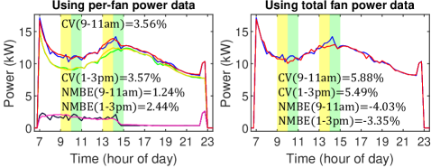
Figure 8: Actual and approximated per-fan and$/$or total fan power traces based on per-fan power data and total fan power data (BBB, Aug. 14, 2017).

Here, we apply the tensor completion method to total fan power data obtained by summing the original per-fan data across fans. Fig. 7 shows the error metrics, based on 15-minute interval data, obtained using per-fan data versus total fan power data. The tensor completion method with per-fan power data outperforms the degenerate version of the method with total fan power data. This result supports the use of our 3-dimensional per-fan power data based tensor completion method, i.e., baselining total fan power according to dominant per-fan power patterns that are consistent among different fans and over different days.

Fig. 8 shows an example of the per-fan and total fan power traces approximated by the tensor completion method with per-fan data, and the total fan power trace approximated by the degenerate version of the method with total fan power data. As shown in Fig. 8 (Left), the proposed method approximates power traces of supply fan 1 and return fan 1, which are summed to approximate the total fan power. During event windows where the approximation acts as the estimated baseline, the per-fan estimations are smooth. The positive and negative errors somewhat balance each other out over time, and the estimation errors of two fans generally balance each other out. The resulting total fan power baseline has lower CV and NMBE. The other case in Fig. 8 (Right) that directly approximates the total fan power trace produces a less smooth baseline estimate and also higher CV and NMBE.

IV-C Huber Loss Function versus $L_{2}$-Norm Loss Function

Figure 9: Mean values of CV and NMBE of the tensor completion method with the Huber and $L_{2}$-norm loss functions. (The error bars represent standard deviations.)

Figure 10: Boxplots of CV and AEC for different building-years. (BL1: Tensor; BL2: Linear interpolation; BL3: 5-day average; BL4: Nearest3of6.)

Here, we test the $L_{2}$-norm loss function and compare it to the Huber loss function, used to generate the previous results. Fig. 9 shows the comparison using 15-min interval per-fan power data. For building-years BBB-2017, RAC-2017 and RAC-2018, the two loss functions produce comparable results, with the Huber loss function producing slightly better results in general. However, for BBB-2018 and WH-2017, the $L_{2}$-norm loss function produces results with much larger baseline errors. BBB-2018 is the smallest data set, with only 16 baseline days. It has an obvious outlier on one baseline day when 6 fans suddenly stop working for about 30 minutes. WH-2017 is the largest data set, but with more visible outliers than other building-years. For example, its day mode HVAC operational period is normally 5am-5pm or 4am-9pm; however, on several days the period is different from the normal ones and also different from the other abnormal ones. These results imply higher robustness to outliers with the Huber loss function compared to the $L_{2}$-norm loss function.

IV-D Comparison with Other Baseline Methods

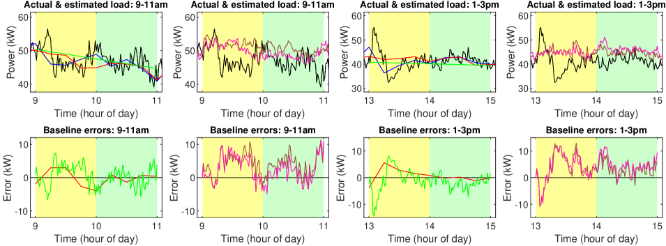
Figure 11: Actual and estimated total fan power baselines and the estimation errors (WH, Jul. 19, 2017). CV(9-11am) of the tensor completion method$/$linear interpolation method$/$5-day average method$/$nearest3of6 method are: 5.50%$/$6.66%$/$10.93%$/$9.65%; CV(1-3pm): 6.95%$/$9.68%$/$13.69%$/$14.59%; AEC(9-11am): -0.601kWh$/$0.832kWh$/$7.974kWh$/$5.090kWh; AEC(1-3pm): 1.449kWh$/$-2.392kWh$/$7.088kWh$/$8.437kWh.

TABLE III: AEC of the Tensor Completion Method and Linear Interpolation Method

		Tensor completion	Linear interpolation
AEC (kWh), 9-11am: Bias$\pm$95%CI	BBB-2017	-0.056 $\pm$ 0.243	0.390 $\pm$ 0.273
	BBB-2018	-0.529 $\pm$ 1.732	1.543 $\pm$ 1.007
	RAC-2017	-1.034 $\pm$ 1.368	-0.728 $\pm$ 0.885
	RAC-2018	0.288 $\pm$ 1.387	0.664 $\pm$ 1.624
	WH-2017	-0.495 $\pm$ 1.685	-3.815 $\pm$ 2.016
AEC (kWh), 1-3pm: Bias$\pm$95%CI	BBB-2017	-0.105 $\pm$ 0.361	-0.786 $\pm$ 0.261
	BBB-2018	0.433 $\pm$ 2.427	-0.192 $\pm$ 0.928
	RAC-2017	-0.059 $\pm$ 0.243	-0.051 $\pm$ 0.194
	RAC-2018	-0.603 $\pm$ 1.380	-0.060 $\pm$ 0.474
	WH-2017	-0.729 $\pm$ 1.532	-2.510 $\pm$ 1.349

Next, we compare the tensor completion method (using 15-minute interval per-fan power data and the Huber loss function) with three other baseline methods: 1) Linear interpolation [5] [6]: This method uses least squares to fit a linear baseline to the total fan power data over the 5-minute periods just before and immediately after the event window. 2) 5-day average [26]: The average load over the 5 most recent baseline days is used to estimate the baseline. 3) Nearest3of6 [3]: Among the 6 most recent baseline days, the 3 days with electricity consumption outside of event windows that is closest to that on the event day are averaged to estimate the baseline. Following [3], the three benchmark methods use 1-minute interval total fan power data here. The impact of data granularity on the benchmark methods’ performance will be explored in future work. A simple additive adjustment, which vertically shifts the baseline estimate so that it is equal to the actual load just prior to the event window, is also applied to the latter two methods [3].

Fig. 10 shows the comparison. The tensor completion method and linear interpolation method have better performance than the 5-day average and Nearest3of6 methods. The tensor completion method generally outperforms the linear interpolation method for BBB-2017, BBB-2018 and WH-2017. For RAC-2017 and RAC-2018 their accuracy is similar. Fig. 11 shows an example of the actual and estimated total fan power baselines. As can be seen, the two averaging methods do not estimate the minute-scale variation of the actual baseline very well, producing larger errors. The linear interpolation method does not capture the variation at all. Instead, it expects positive and negative errors to balance out over time, which is appropriate for some DR applications that only need the average deviation over the event. In this example, it performs well; however, the tensor completion method outperforms it.

Table III reports mean values and 95% confidence intervals for the AEC for the tensor completion method and linear interpolation method. The 95% confidence intervals are calculated by ${\color[rgb]{0,0,0}\operatorname{mean}}(AEC)\pm 1.96\times{\color[rgb]{0,0,0}\operatorname{std}}(AEC)/\sqrt{S}$, where $S$ denotes the number of baseline days in a data set that the baseline method is tested on. Note that the bias of AEC is especially important for DR applications such as financial settlement. Table III indicates that the tensor completion method generally outperforms the linear interpolation method in baselining fan power within the morning event window, while the interpolation method is generally better within the afternoon event window. Still, the tensor completion method has a more consistent performance, while the interpolation method ends up with a much larger bias in BBB-2018 (for the morning event window) and WH-2017 (for both event windows).

V Conclusions and Future Work

This paper investigated the use of tensor completion for baseline estimation of commercial building HVAC system fan power. The proposed method estimates baseline fan power by forming a tensor from submetered per-fan power data and then imputing the counterfactual measurements from DR event windows to encourage correlations along the dimensions of time, fan, and day. These estimates of counterfactual fan power are taken from a low-rank GCP tensor decomposition that approximates the fan power data tensor on measurements of baseline days and of the event day but outside DR event window(s). We compared the proposed method with the linear interpolation, 5-day average, and Nearest3of6 methods using data collected at the University of Michigan and found that the proposed method generally has the best performance.

An important direction for future work is developing methods for selecting the tensor rank. Various methods might be considered, e.g., one could select the rank that best estimates the measurements on a validation set of the data, but more work is needed to assess and understand the trade-off between data overfit and approximation error discussed in Section III-B. These tradeoffs can also be influenced if we incorporate regularization in the GCP tensor decomposition objective 3 as described in [13, Section 4.2]. For example, regularizing the temporal factors of $\boldsymbol{\widehat{\mathscr{P}}}$ to be piecewise smooth may help mitigate data overfit, allowing for decompositions of higher ranks.

Another avenue for future work is to consider other tensor completion approaches, such as those described in the recent survey [12]. In particular, many approaches exploit low-rank structure with respect the Tucker decomposition [7, Section 4], e.g., [27] is a recent proposal based on Tucker rank. Exploring these tensor completion approaches and their tradeoffs is an important and promising direction.

References

- [1] H. Hao, Y. Lin, A. S. Kowli, P. Barooah, and S. Meyn, “Ancillary service to the grid through control of fans in commercial building HVAC systems,” IEEE Trans. Smart Grid, vol. 5, no. 4, pp. 2066–2074, Jul. 2014.
- [2] F. Wang, K. Li, C. Liu, Z. Mi, M. Shafie-Khah, and J. P. S. Catalão, “Synchronous pattern matching principle-based residential demand response baseline estimation: Mechanism analysis and approach description,” IEEE Trans. Smart Grid, vol. 9, no. 6, pp. 6972–6985, Nov. 2018.
- [3] S. Lei, J. L. Mathieu, and R. K. Jain, “Performance of existing baseline models in quantifying the effects of short-term load shifting of campus buildings,” SLAC National Accelerator Laboratory, Tech. Rep., SLAC-R-1131, Menlo Park, CA USA, Aug. 2019. [Online]. Available: https://www.slac.stanford.edu/pubs/slacreports/reports21/slac-r-1131.pdf
- [4] Y. Zhang, W. Chen, R. Xu, and J. Black, “A cluster-based method for calculating baselines for residential loads,” IEEE Trans. Smart Grid, vol. 7, no. 5, pp. 2368–2377, Sep. 2016.
- [5] I. Beil, I. A. Hiskens, and S. Backhaus, “Round-trip efficiency of fast demand response in a large commercial air conditioner,” Energy Build., vol. 97, pp. 47–55, Jun. 2015.
- [6] A. Keskar, D. Anderson, J. X. Johnson, I. A. Hiskens, and J. L. Mathieu, “Experimental investigation of the additional energy consumed by building HVAC systems providing grid ancillary services,” in Proc. 20th ACEEE Summer Study Energy Effic. in Build., Pacific Grove, CA, Aug. 2018, pp. 1–12.
- [7] T. G. Kolda and B. W. Bader, “Tensor decompositions and applications,” SIAM Review, vol. 51, no. 3, pp. 455–500, Aug. 2009.
- [8] K. Maruhashi, F. Guo, and C. Faloutsos, “Multiaspectforensics: Pattern mining on large-scale heterogeneous networks with tensor analysis,” in Proc. 2011 Int. Conf. Advances in Social Netw. Anal. & Min., Taiwan, China, Jul. 2011, pp. 203–210.
- [9] N. Batra, Y. Jia, H. Wang, and K. Whitehouse, “Transferring decomposed tensors for scalable energy breakdown across regions,” in Proc. 32nd AAAI Conf. Artif. Intell., New Orleans, LA, Feb. 2018, pp. 1–8.
- [10] D. Osipov and K. Sun, “Tensor decomposition based adaptive model reduction for power system simulation,” Accepted to 2020 IEEE Power & Energy Society General Meeting, Montreal, Canada, Aug. 2020.
- [11] D. Hong, S. Lei, J. L. Mathieu, and L. Balzano, “Exploration of tensor decomposition applied to commercial building baseline estimation,” in Proc. 7th IEEE Global Conf. Signal & Inf. Process. (GlobalSIP), Ottawa, Canada, Nov. 2019, pp. 1–5.
- [12] Q. Song, H. Ge, J. Caverlee, and X. Hu, “Tensor completion algorithms in big data analytics,” ACM Trans. Knowl. Discov. Data, vol. 13, no. 1, pp. 1–48, Jan. 2019.
- [13] D. Hong, T. G. Kolda, and J. A. Duersch, “Generalized canonical polyadic tensor decomposition,” SIAM Review, vol. 62, no. 1, pp. 133–163, Feb. 2020.
- [14] A. Keskar, D. Anderson, J. X. Johnson, I. A. Hiskens, and J. L. Mathieu, “Do commercial buildings become less efficient when they provide grid ancillary services?” Energy Efficiency, Apr. 2019.
- [15] P. J. Huber, “Robust estimation of a location parameter,” Ann. Math. Statist., vol. 35, no. 1, pp. 73–101, Mar. 1964.
- [16] T. Hastie, R. Tibshrirani, and J. Friedman, The Elements of Statitical Learning, 2nd ed., Springer, 2009.
- [17] B. W. Bader, T. G. Kolda et al., “MATLAB Tensor Toolbox Version 3.1,” Jun. 2019. [Online]. Available: https://www.tensortoolbox.org
- [18] R. H. Byrd, P. Lu, J. Nocedal, and C. Zhu, “A limited memory algorithm for bound constrained optimization,” SIAM J. Sci. Comput., vol. 16, no. 5, pp. 1190–1208, Sep. 1995.
- [19] J. B. Kruskal, “Rank, decomposition, and uniqueness for 3-way and n-way arrays,” in Multiway Data Analysis, 1989, pp. 7–18.
- [20] R. K. Jain, K. M. Smith, P. J. Culligan, and J. E. Taylor, “Forecasting energy consumption of multi-family residential buildings using support vector regression: Investigating the impact of temporal and spatial monitoring granularity on performance accuracy,” Appl. Energy, vol. 123, pp. 168–178, Jun. 2014.
- [21] R. Sevlian and R. Rajagopal, “A scaling law for short term load forecasting on varying levels of aggregation,” Int. J. Elec. Power & Energy Syst., vol. 98, pp. 350–361, Jun. 2018.
- [22] M. Sun, Y. Wang, F. Teng, Y. Ye, G. Strbac, and C. Kang, “Clustering-based residential baseline estimation: A probabilistic perspective,” IEEE Trans. Smart Grid, vol. 10, no. 6, pp. 6014–6028, Nov. 2019.
- [23] “ASHRAE Guideline 14–2014: Measurement of energy, demand, and water savings,” American Society of Heating, Ventilating, and Air Conditioning Engineers, Tech. Rep., Atlanta, GA, USA, Dec. 2014. [Online]. Available: https://www.ashrae.org/technical-resources/standards-and-guidelines/titles-purposes-and-scopes
- [24] R. E. Edwards, J. New, and L. E. Parker, “Predicting future hourly residential electrical consumption: A machine learning case study,” Energy Build., vol. 49, pp. 591–603, Jun. 2012.
- [25] J. L. Mathieu, D. S. Callaway, and S. Kiliccote, “Variability in automated responses of commercial buildings and industrial facilities to dynamic electricity prices,” Energy Build., vol. 43, no. 12, pp. 3322–3330, Dec. 2011.
- [26] K. Coughlin, M. A. Piette, C. Goldman, and S. Kiliccote, “Statistical analysis of baseline load models for non-residential buildings,” Energy Build., vol. 41, no. 4, pp. 374–381, Apr. 2009.
- [27] A. Zhang, “Cross: Efficient low-rank tensor completion,” Ann. Statist., vol. 47, no. 2, pp. 936–964, 2019.