Propagation of gravitational waves in various cosmological backgrounds

Abstract

The present work investigates some exact solutions of the gravitational wave equation in some widely used cosmological spacetimes. The examples are taken from spatially flat and closed isotropic models as well as Kasner metric which is anisotropic. Various matter distributions are considered, from the standard dust or radiation distribution to exotic matters like that with an equation of state $P=-\frac{1}{3}\rho$. In almost all cases the frequency and amplitude of the wave are found to be decaying with evolution, except for a closed radiation universe where there is a resurgence of the waveform, consistent with the recollapse of the universe into the big crunch singularity.

1 Introduction

Albeit the indirect evidence of gravitational waves came through the observations by Hulse and Taylor of a binary pulsar [1] in 1974, the direct detection of the same was possible only very recently, when the LIGO and VIRGO scientific collaboration announced their first direct observation of gravitational wave in 2016 [2]. This discovery, not only a great triumph of a relativistic theory of gravitation, but also opened up a completely new window for the exploration of the universe. We can analyze the properties of gravitational waves to study various extreme astrophysical objects like black holes [2, 3, 4], neutron stars [5] and also may be able to extract various cosmological information [6] from these gravitational waves.

As some of the detected gravitational waves might have travelled through a great distance of a few billion parsecs, such as GW170729 (see the work of Abbott et al [7]), the curvature of cosmological background might well have its imprint on the waves. The cosmological signature could also be small, and might not have any significant observational implications in near future, but the estimated distance travelled by them strongly indicates that one needs to ascertain the difference of the waveforms travelled through the cosmic fluid or through vacuum where the imprints of cosmology is neglected at the outset.

No wonder that the investigations along this direction of research is already under way. The foundation of such investigations had been in the literature for quite a long time back [8]. Mendes and Liddle[9] examined the possible effect of the events in the early universe, such as the early inflation or even the possibility of a second burst of inflation at the onset of matter domination, on the stochastic gravity wave background. Seto and Yokoyama worked on the effect of the equation of state of the matter content of the universe in its early stages[10]. Kuroyanagi, Takahashi and Yokoyama[11] discussed the features of the early universe by looking at the constraints on the primordial gravity waves. Capozziello, Laurentis and Francaviglia considered gravity waves in a cosmological background in higher order gravity[12].

However, the interest naturally proliferated after the direct detection of gravitational waves. Very recently Valtancoli [13] discussed the gravitational wave propagation in an AdS spacetime and argued that the graviton mass cannot be measured with precision more than $\sqrt{\Lambda}$. Kulczycki and Malec [14] showed that for a smooth initial metric, with certain differentiability conditions, gives rise to gravitational wave pulses that do not interact with the background in the radiation dominated era. Possible effects of gravitational waves on the dark energy dominated era have been investigated by Creminelli and Vernizzi [15] and the effect of the waves in connection with structure formation was looked at by Jimenez and Heisenberg [16]. Caldwell and Devulder worked on the possible opacity for gravitational waves by a particular form of dark energy and showed that the maximum absorption is around $1\%$ for the redshift range $0.5\leq z\leq 1.5$ [17]. Most of these investigations are based on spatially flat isotropic cosmologial background. Bradley, Forsberg and Keresztes [18] discussed the propagation of gravitational waves in a class of locally rotationally symmetric spacetime. There are some work on the propagation of such waves in relativistic theories of gravity other than general relativity also, such as in Jordan-Brans-Dicke theory[19], in teleparallel gravity[20], in a general scalar-tensor theory[21]. Evolution of gravitons in an accelerating in an extended gravity theory was discussed by Capozziello et al [22].

The motivation of the present work is to look at the wave forms travelling in a cosmological background, through the cosmic fluid. We do not bother about source of the wave, but rather concentrate on the exact solutions of the wave equation in the linear regime of the perturbation. But the investigation is not restricted to a spatially flat isotropic cosmology only. From the general equation for the gravitational wave, we write down the equations for some given cosmology, namely a spatially flat FRW cosmology, a spatially closed FRW cosmology and an anisotropic cosmology. We neglect the perturbation in the matter sector, and consider only the metric perturbation giving rise to perturbations in the curvature. In some well known examples of cosmological models, we could actually find the exact solutions to the wave equation. For some choices of the constants of integrations, we plot the wave form. The interest in this work is to look at the features qualitatively, so actual numbers related to various parameters are chosen for the sake of convenience so as to get exact solutions. As expected, in most cases both the amplitude and frequency die down with time, with one exception of a spatially closed model where the wave form has a resurgence with the recollapse of the universe.

The closest to this present work is the one by Flauger and Weinberg [23], which deals with the propagation in a cold dark matter (CDM). They predict that the magnitude of the cosmic effect is too small to influence the observations. This is attributed by them to the fact that the CDM is too nonrelativistic to affect the wave. They also show that for a primordial wave, the imprints are more pronounced for the intermediate modes. We, however, looked at various kinds of matter distribution including very highly relativistic matter like a radiation distribution.

The outline of the paper is as follows. We begin with a brief review of the general formulation involved in the propagation of gravitational wave in Sec. II and write down the wave equation of the gravitational wave in a general curved background. In Sec. III, we consider the spatially homogeneous and isotropic universe. The equations for the gravitational wave for the FRW universe are written and exact solutions are obtained for spatially flat and spatially closed FRW universe for some given matter distributions. In Sec. IV we discuss about the wave propagation in an anisotropic universe by considering Bianchi universe. The exact solutions for a particular orientation of propagation are obtained for a Kasner metric. A discussion of the results obtained are given in the fifth and final section.

2 The General Formulation

We begin by writing the equation for the metric perturbations in a general curved spacetime whose solution will finally yield the gravitational wave profile for the given spacetime. The procedure is standard and is discussed in standard texts like [24]. One can also refer to [25, 26]. We shall consider a non-zero background stress-energy tensor. The perturbed metric is written as

$$g_{\mu\nu}=\gamma_{\mu\nu}+\epsilon h_{\mu\nu},$$ (1)

where $\epsilon$ is a small parameter which makes $\epsilon h_{\mu\nu}$ a small perturbation to $\gamma_{\mu\nu}$, which is the background metric. Raising and lowering of indices will take place through the background metric $\gamma_{\mu\nu}$. The inverse of the metric, i.e., $g^{\mu\nu}$, can be written as (up to linear order)

$$g^{\mu\nu}=\gamma^{\mu\nu}-\epsilon h^{\mu\nu}.$$ (2)

Unlike Minkowski background, where the perturbation is considered to be small compared to unity, the isolation of the perturbation from the background is not so trivial. This is primarily because both $\gamma_{\mu\nu}$ and $h_{\mu\nu}$ are functions of coordinates. What one normally considers in this case a short wave or high frequency condition where the wavelength ($\lambda$) of the perturbation, which satisfies a wave equation, is much smaller compared to the typical length scale ($L$) of the backgroumd. It can be shown that the first order correction to the Christoffel symbol $\Gamma$ (called $\Gamma^{(1)}$ in the present discussion) and the first order correction to the Ricci curvature ($R^{(1)}$) corresponds to the short wave. For an elaborate calculation, we refer to the comprehensive book by Maggiore[27].

Using the equations (1) and (2) in the expression of the Christoffel symbol, one can obtain

$$\Gamma^{\rho}_{\mu\nu}= \overline{\Gamma}^{\rho}_{\mu\nu}+\frac{1}{2}\gamma^{\rho\sigma}[\nabla_{\nu}h_{\mu\sigma}+\nabla_{\mu}h_{\sigma\nu}-\nabla_{\sigma}h_{\mu\nu}]$$ (3)

$$= \overline{\Gamma}^{\rho}_{\mu\nu}+\Gamma^{\rho(1)}_{\mu\nu}.$$ (4)

We will deal with only the terms that are linear in $\epsilon$ and hence the use of term $\epsilon$ is absorbed in the components $h^{\mu\nu}$ which themselves will take care of being small. We can clearly see that in the case of curved background spacetime, the Christoffel symbols break down into two distinct parts, one is the background spacetime Christoffel symbols which are denoted by the $\overline{\Gamma}$ and the another one is linearly perturbed Christoffel symbols which are denoted as $\Gamma^{(1)}$. One can use the Christoffel symbols to obtain Riemann tensor. We write the Riemann tensor as a sum of the background Riemann tensor and the linearly perturbed Riemann tensor as

$${R^{\rho}}_{\mu\nu\lambda}={\overline{R}^{\rho}}_{\mu\nu\lambda}+{R^{(1)\rho}}_{\mu\nu\lambda}.$$ (5)

The linearly perturbed part of Ricci tensor can now be written as

$$R^{(1)}_{\alpha\beta}=\frac{1}{2}\left[\nabla_{\rho}\nabla_{\alpha}h^{\rho}_{\beta}+\nabla_{\rho}\nabla_{\beta}h^{\rho}_{\alpha}-\Box h_{\alpha\beta}-\nabla_{\beta}\nabla_{\alpha}h\right].$$ (6)

In the above equation $h=h^{\mu}_{\mu}$ is the trace of the metric perturbation.

In a similar fashion we can divide Einstein tensor, and hence the Einstein field equation, into its background part $\overline{G}_{\alpha\beta}$ and the linearly perturbed part $G^{(1)}_{\alpha\beta}$ as follows

$$G_{\alpha\beta} =\overline{G}_{\alpha\beta}+G^{(1)}_{\alpha\beta}$$ (7)

$$=-8\pi T_{\alpha\beta}$$ (8)

$$=-8\pi\left(\overline{T}_{\alpha\beta}+T_{\alpha\beta}^{(1)}\right),$$ (9)

where the $\overline{T}_{\alpha\beta}$ is the background stress-energy tensor and $T_{\alpha\beta}^{(1)}$ is the linear order perturbations of stress-energy tensor. From the above discussion of order of magnitude, we consider the perturbation of stress-energy tensor to be zero, i.e. $T^{(1)}_{\alpha\beta}=0$. So one has $G^{(1)}_{\alpha\beta}=0$.

This requires some explanation. As shown in [27], the first order correction to the stress energy tensor actually contributes to long wave (or small frequency) and not to the short wave condition ($\lambda<<L$) and thus not of relevance for the present discussion as discussed in the beginning of this section.

If we take the trace of Einstein equation, we get $R^{(1)}=-8\pi T^{(1)}=0$ and hence, we get $R^{(1)}_{\alpha\beta}=0$. Therefore, the expression of $R^{(1)}_{\alpha\beta}$ (6), leads to

$$R^{(1)}_{\alpha\beta}=\frac{1}{2}\left[\nabla_{\rho}\nabla_{\alpha}h^{\rho}_{\beta}+\nabla_{\rho}\nabla_{\beta}h^{\rho}_{\alpha}-\Box h_{\alpha\beta}-\nabla_{\beta}\nabla_{\alpha}h\right]=0.$$ (10)

The above equation can be simplified using the trace-reversed perturbation variable. The trace-reversed perturbation variable is defined as $\tilde{h}_{\mu\nu}=h_{\mu\nu}-\frac{1}{2}\gamma_{\mu\nu}h.$ As $\tilde{h}=-h$, where $\tilde{h}=\tilde{h}^{\mu}_{\mu}$ and $h=h^{\mu}_{\mu}$, we have $h_{\mu\nu}=\tilde{h}_{\mu\nu}-\frac{1}{2}\gamma_{\mu\nu}\tilde{h}.$ One can replace the perturbation variable with the trace-reversed perturbation variable, as a result, the equation (10) reduces to

$$\nabla_{\rho}\nabla_{\alpha}\tilde{h}^{\rho}_{\beta}+\nabla_{\rho}\nabla_{\beta}\tilde{h}^{\rho}_{\alpha}-\Box\tilde{h}_{\alpha\beta}+\frac{1}{2}\gamma_{\alpha\beta}\Box\tilde{h}=0.$$ (11)

The equation (11) can be further simplified by using a suitable gauge. In the case of curved background spacetime, the modified Lorenz gauge can be written as

$$\nabla_{\nu}\tilde{h}^{\mu\nu}=0.$$ (12)

It may be noted that the corresponding equation given in [11] looks different from this equation, which is simply because the present work uses the cosmic time $t$ as opposed to the conformal time $\tau$ used in [11]. A transformation of the form $dt=a(\tau)d\tau$ in the present equation resolves the apparent mismatch. We can modify the first and second terms in the equation (11) in terms of Riemann and Ricci tensors. Using Lorenz gauge, equation (11) reduces to

$$\bar{R}_{\delta\alpha}\tilde{h}^{\delta}_{\beta}+\bar{R}_{\delta\beta}\tilde{h}^{\delta}_{\alpha}-2\bar{R}_{\beta\delta\alpha\rho}\tilde{h}^{\delta\rho}-\Box\tilde{h}_{\alpha\beta}+\frac{1}{2}\gamma_{\alpha\beta}\Box\tilde{h}=0.$$ (13)

Apart from the Lorenz gauge, we also impose the condition that gravitational wave is traceless, and therefore we have $\tilde{h}=\tilde{h}^{\alpha}_{\alpha}=0$. Using the traceless condition in equation (13), we obtain the final wave equation for the gravitational wave in the curved background spacetime as

$$\Box\tilde{h}_{\beta\alpha}-2\bar{R}_{\delta\beta\alpha\rho}\tilde{h}^{\delta\rho}-\bar{R}_{\delta\alpha}\tilde{h}^{\delta}_{\beta}-\bar{R}_{\delta\beta}\tilde{h}^{\delta}_{\alpha}=0.$$ (14)

It may be mentioned that in the equations (13, 14), the effect of the matter distribution on the gravitational wave propagation is taken care of by the Ricci tensor through the background Einstein equations, while the Riemann tensor determines the contribution due to the background curvature.

3 Gravitational waves in FRW universe

In this section we investigate the propagation of gravitational waves in a cosmological background which is spatially homogeneous and isotropic. The corresponding spacetime is described by the Friedmann, Robertson and Walker (FRW) metric

$$ds^{2}=-dt^{2}+a^{2}(t)\left[\frac{dr^{2}}{1-kr^{2}}+r^{2}d\theta^{2}+r^{2}\sin^{2}\theta d\phi^{2}\right],$$ (15)

where $k$ denotes the spatial curvature and takes values $0,+1,-1$ for spatially flat, closed and open universe respectively.

3.1 Background equations

The function $a(t)$ is known as the scale factor and is governed, when the universe is filled with a perfect fluid, by the equations

$$\frac{\ddot{a}}{a} =-\frac{4\pi}{3}(\rho+3p)$$ (16)

$$\left(\frac{\dot{a}}{a}\right)^{2} =\frac{8\pi}{3}\rho-\frac{k}{a^{2}}.$$ (17)

For a given equation of state $P=P(\rho)$, these equations can be integrated to find the dynamics of the background metric.

3.2 Gravitational wave equations

To derive gravitational wave equations in FRW spacetime we use the equation (14) along with the relevant Riemann and Ricci tensor components which are computed using the FRW metric (15). For brevity of notations, now onward we shall use $h_{\alpha\beta}$ instead of $\tilde{h}_{\alpha\beta}$ to denote metric perturbation components. In particular, the gravitational wave equations in spherical polar coordinates, can be explicitly expressed as

$$\Box{h}_{00}-2\left[\frac{\ddot{a}(1-kr^{2})}{a^{3}}{h}_{11}+\frac{\ddot{a}}{a^{3}r^{2}}{h}_{22}+\frac{\ddot{a}}{a^{3}r^{2}\sin^{2}{\theta}}{h}_{33}\right]-6\frac{\ddot{a}}{a}{h}_{00}=0,$$ (18)

$$\Box{h}_{11}-2\left[\frac{\dot{a}^{2}+k}{a^{2}r^{2}(kr^{2}-1)}{h}_{22}+\frac{\dot{a}^{2}+k}{(kr^{2}-1)a^{2}r^{2}\sin^{2}\theta}{h}_{33}-\frac{a\ddot{a}}{kr^{2}-1}{h}_{00}\right]-2\left[2\frac{\dot{a}^{2}}{a^{2}}+2\frac{k}{a^{2}}+\frac{\ddot{a}}{a}\right]{h}_{11}=0,$$ (19)

$$\Box{h}_{22}+2\left[\frac{r^{2}(\dot{a}^{2}+k)(1-kr^{2})}{a^{2}}{h}_{11}+\frac{(\dot{a}^{2}+k)}{a^{2}\sin^{2}\theta}{h}_{33}-r^{2}a\ddot{a}{h}_{00}\right]-2\left[2\frac{\dot{a}^{2}}{a^{2}}+2\frac{k}{a^{2}}+\frac{\ddot{a}}{a}\right]{h}_{22}=0,$$ (20)

$$\Box{h}_{33}-2\left[r^{2}a\ddot{a}\sin^{2}\theta{h}_{00}-\frac{(1-kr^{2})r^{2}\sin^{2}\theta(\dot{a}^{2}+k)}{a^{2}}{h}_{11}-\frac{\sin^{2}\theta(\dot{a}^{2}+k)}{a^{2}}{h}_{22}\right]-2\left[2\frac{\dot{a}^{2}}{a^{2}}+2\frac{k}{a^{2}}+\frac{\ddot{a}}{a}\right]{h}_{33}=0,$$ (21)

$$\Box{h}_{0i}-\left[6\frac{\ddot{a}}{a}+2\frac{\dot{a}^{2}}{a^{2}}+\frac{2k}{a^{2}}\right]{h}_{0i}=0,\text{ for}\ i=1,2,3,$$ (22)

$$\Box{h}_{mn}-\left[2\frac{\ddot{a}}{a}+6\frac{\dot{a}^{2}}{a^{2}}+\frac{6k}{a^{2}}\right]{h}_{mn}=0,\text{ for}\ m,n=1,2,3\text{ and}\ m\neq n.$$ (23)

Here $x^{1},x^{2},x^{3}$ correspond to the coordinates $r,\theta,\phi$ respectively.

3.3 Solutions to the gravitational wave equations

3.3.1 Spatially flat FRW universe

In spatially flat FRW spacetime, it is convenient to use Cartesian coordinate system, which allows us use transverse-traceless-synchronous (TTS) gauge [28, 29] efficiently. We choose that the wave is propagating along the $x$ direction. So according to TTS gauge, $h_{0\mu}$ and ${h}_{1\mu}$ are zero, and ${h}_{22}=-{h}_{33}$, where the subscript $0,1,2,3$ denotes $t,x,y,z$ coordinates respectively. After applying the TTS gauge, the number of nonzero and independent wave equations reduce to two, which are given by

$$\Box{h}_{22}-\left[2\frac{\ddot{a}}{a}+6\frac{\dot{a}^{2}}{a^{2}}\right]{h}_{22} = 0$$ (24)

$$\Box{h}_{23}-\left[2\frac{\ddot{a}}{a}+6\frac{\dot{a}^{2}}{a^{2}}\right]{h}_{23} = 0.$$ (25)

We shall investigate the evolution of gravitational waves in a dust dominated as well as radiation dominated universe.

For the dust ($P=0$) dominated spatially flat FRW universe, the scale function grows with time as

$$a=a_{i}~{}t^{\frac{2}{3}}~{},$$ (26)

where $a_{i}$ is a constant. Now we consider an ansatz that the perturbation components are function of $t$ and $x$ only. As equations (24) and (25) are similar in form, so it is sufficient to solve one of them. We take ${h}_{22}=\Psi(x,t)$. Equation (24) will now look like

$$\frac{\partial^{2}\Psi}{\partial t^{2}}+3\frac{\dot{a}}{a}\frac{\partial\Psi}{\partial t}-\frac{1}{a^{2}}\frac{\partial^{2}\Psi}{\partial x^{2}}-\left(2\frac{\ddot{a}}{a}+6\frac{\dot{a}^{2}}{a^{2}}\right)\Psi=0.$$ (27)

For dust dominated universe, we can use the expression of scale factor from equation (26), in equation (27) to get the wave equation as

$$\frac{\partial^{2}\Psi}{\partial t^{2}}+\frac{2}{t}\Psi-\frac{1}{a_{i}^{2}t^{\frac{4}{3}}}\frac{\partial^{2}\Psi}{\partial x^{2}}-\frac{20}{9t^{2}}\Psi=0.$$ (28)

One can solve this equation by using separation of variable as $\Psi(x,t)=X_{1}(x)T_{1}(t)$. The equation (28) will break as

$$a_{i}^{2}t^{\frac{4}{3}}\left(\frac{1}{T_{1}}\frac{d^{2}T_{1}}{dt^{2}}+\frac{2}{t}\frac{1}{T_{1}}\frac{dT_{1}}{dt}-\frac{20}{9t^{2}}\right)=\frac{1}{X_{1}}\frac{d^{2}X_{1}}{dx^{2}}=-{\Omega^{2}}~{},$$ (29)

where ${\Omega^{2}}$ is the separation constant.The choice of the sign of the separation constant is negative as we are looking for a periodic variation. From equation (29), we can see that the solution of the spatial part is given by

$$X_{1}(x)=E\cos(\Omega x)+F\sin(\Omega x),$$ (30)

where $E$ and $F$ are constant of integration. The temporal part of the equation is

$$\frac{d^{2}T_{1}}{dt^{2}}+\frac{2}{t}\frac{dT_{1}}{dt}+\left(\frac{{\Omega^{2}}}{a_{i}^{2}t^{\frac{4}{3}}}-\frac{20}{9t^{2}}\right)T_{1}=0.$$ (31)

The solution of the above equation is

$$\begin{split}T_{1}(t)=\frac{2\sqrt{\frac{2}{3}}a_{i}^{\frac{3}{2}}}{3\sqrt{t}{\Omega}^{\frac{3}{2}}}\left[C_{1}\Gamma\left(1-\frac{\sqrt{89}}{2}\right)J_{-\frac{\sqrt{89}}{2}}\left(\frac{3\sqrt[3]{t}{\Omega}}{a_{i}}\right)\right.\\ +\left.C_{2}\Gamma\left(1+\frac{\sqrt{89}}{2}\right)J_{\frac{\sqrt{89}}{2}}\left(\frac{3\sqrt[3]{t}{\Omega}}{a_{i}}\right)\right].\end{split}$$ (32)

Here $C_{1}$ and $C_{2}$ are the constants of integration, $J_{n}(z)$ and $\Gamma(z)$ are Bessel function of first kind of order $n$ and gamma function respectively. The plot of the evolution of gravitational wave with time is given by FIG. 1, where the constant $a_{i}$ is taken as $1$ without any loss of generality. The unit of time needs some attention. In the metric (15), as $k$ is dimensionless, the radial coordinate $r$ is scaled by some $r_{0}$. The time is actually scaled by some $t_{0}$, so that all the quantities in the metric are dimensionless, which is quite a standard practice. From equation (26), one can ascertain $t_{0}=a_{i}$, which is chosen to be unity. With this, one can see that the unit of time is chosen to be $H_{0}^{-1}$ multiplied by a constant of order unity (such as $\frac{2}{3}$ for dust and $\frac{1}{2}$ for radiation etc). $H_{0}$ is the Hubble parameter $H=\frac{\dot{a}}{a}$ evaluated at $a=a_{i}=1$. In all the plots, the amplitude is scaled by its initial value.

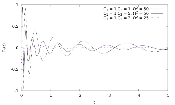
Figure 1: Plot of evolution of gravitational wave with time in a dust matter dominated spatially flat universe.

From the plot we see that the amplitude of the wave decays and the frequency of the wave also decreases with time. One may understand that the damping is due to the expansion of the universe, which describes the behaviour of the gravitational waves in an expanding universe with respect to a co-moving observer.

For a radiation dominated universe, with the equation of state being $P=\frac{1}{3}\rho$, the scale function grows as

$$a=a_{i}t^{\frac{1}{2}}.$$ (33)

As earlier, by choosing $a_{i}=1$ and using the separation of variables ${\Psi}_{2}=X_{2}(x)T_{2}(t)$, one may note that the spatial part is the same as the dust dominated universe, and the solution is given by the equation (30). The temporal evolution equation of the gravitational wave is given by

$$\frac{d^{2}T_{2}}{dt^{2}}+\frac{3}{2t}\frac{dT_{2}}{dt}+\left(\frac{{\Omega^{2}}}{a_{i}^{2}t}-\frac{1}{t^{2}}\right)T_{2}=0~{},$$ (34)

and whose solutions are of the form

$$\begin{split}T_{2}(t)=\frac{\sqrt{a_{i}}}{({\Omega^{2}}t)^{\frac{1}{4}}}\left[C_{3}\Gamma\left(1-\frac{\sqrt{17}}{2}\right)J_{-\frac{\sqrt{17}}{2}}\left(\frac{2\sqrt{t}{\Omega}}{a_{i}}\right)\right.\\ +\left.C_{4}\Gamma\left(1+\frac{\sqrt{17}}{2}\right)J_{\frac{\sqrt{17}}{2}}\left(\frac{2\sqrt{t}{\Omega}}{a_{i}}\right)\right],\end{split}$$ (35)

where $C_{3}$ and $C_{4}$ are constants of integration.

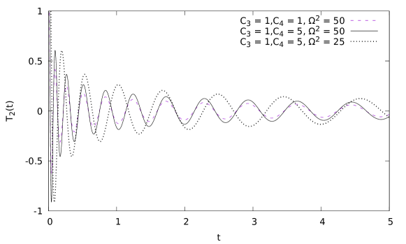
Figure 2: Plot of evolution of gravitational wave with time in a radiation dominated spatially flat universe.

Similar to the evolution of the waveform in a dust dominated universe, here the amplitude and frequency of the wave decreases with time. From FIG. 2, it is quite apparent that the rate of damping of the wave is higher in dust dominated universe than the radiation dominated universe. This is actually consistent as the expansion is faster in the dust dominated universe compared to the radiation dominated universe.

3.3.2 Spatially closed FRW universe

In spatially closed FRW universe, we can again make use of the gauge freedom to reduce the number of the independent equations. For spatially closed universe, system of spherical polar coordinates is the most suitable one to analyze various properties of the universe. We take that the wave propagates in radial direction. We also consider the observer is comoving, so the 4-velocity of the observer is $U^{\mu}=(1,0,0,0)$. In TTS gauge [28, 29] the equations of independent nonzero perturbation components are

$$\Box{h}_{22}-\left[2\frac{\ddot{a}}{a}+6\frac{\dot{a}^{2}}{a^{2}}+\frac{6}{a^{2}}\right]{h}_{22} = 0$$ (36)

$$\Box{h}_{23}-\left[2\frac{\ddot{a}}{a}+6\frac{\dot{a}^{2}}{a^{2}}+\frac{6}{a^{2}}\right]{h}_{23} = 0.$$ (37)

Here the subscript $2$ , $3$ denotes $\theta$ and $\phi$ coordinates respectively in spherical polar coordinate.

We shall investigate the solutions of the gravitational wave equation for two different kinds of evolution, namely the radiation dominated decelerated universe and a coasting universe [30]. For radiation (equation of state $P/\rho=1/3$) dominated spatially closed universe the scale function evolves as

$$a(t)=\zeta\sqrt{1-\left(1-\frac{t}{\zeta}\right)^{2}}.$$ (38)

Here $\zeta=\sqrt{2q_{0}/(2q_{0}-1)}$ is constant and $q=-\ddot{a}/aH^{2}$, is the deceleration parameter of universe and a suffix $0$ indicates its present value. From the equation (38), it is understood that the scale factor grows at a decreasing rate until it stops and gives way to a contraction.

Other than radiation, we shall also discuss about a matter whose equation of state is given by $P/\rho=-1/3$. In various literature this type of matter is described as K-matter [30] or winding modes of a “string gas” [31]. For this type of a matter distribution, the scale factor evolves in terms of cosmic time as [30]

$$a(t)=\sqrt{(K-1)}t=a_{0}H_{0}t.$$ (39)

Here $K=8\pi G{\rho}_{0}{a_{0}}^{2}/3$, and $a_{0}$ and $H_{0}$ are scale factor and Hubble parameter at present time respectively. This evolution has the deceleration parameter $q=0$, which justifies the name a “coasting universe”. From various observational parameters one can constrain the value of $K$ as $K\geq 1.2$ [30].

To solve the gravitational wave equations, we assume that perturbation components are the functions of time($t$) and radial distance($r$) only. As the equations (36) and (37) are same, so it is sufficient to consider only one component of the metric perturbations, namely $h_{22}=\Phi$. With the assumption $\Phi=\Phi(r,t)$, the equation (36) reads as

$$\begin{split}-\frac{\partial^{2}\Phi}{\partial t^{2}}-3\frac{\dot{a}}{a}\frac{\partial\Phi}{\partial t}+\frac{(1-r^{2})}{a^{2}}\frac{\partial^{2}\Phi}{\partial r^{2}}+\frac{(2-3r^{2})}{a^{2}r}\frac{\partial\Phi}{\partial r}\\ -\left[2\frac{\ddot{a}}{a}+6\frac{\dot{a}^{2}}{a^{2}}+\frac{6}{a^{2}}\right]\Phi=0.\end{split}$$ (40)

We can solve this equation by the method of separation of variables, $\Phi(r,t)=R_{3}(r)T_{3}(t)$. The possible solutions of radial part is discussed in literature [32, 33]. The temporal evolution of the wave is given by

$$\frac{d^{2}T_{3}}{dt^{2}}+3\frac{\dot{a}}{a}\frac{dT_{3}}{dt}+\left[2\frac{\ddot{a}}{a}+6\frac{\dot{a}^{2}}{a^{2}}+\frac{(6-{\Omega^{2}})}{a^{2}}\right]T_{3}=0~{},$$ (41)

where ${\Omega^{2}}$ is the separation constant.

For radiation dominated universe the scale factor is given by equation (38). Using equation (38) and (41), we can get the solution of temporal evolution of GW in radiation dominated universe, which is given by

$$T_{3}(t)=\frac{1}{{\sqrt[4]{t}\sqrt[4]{t-2\zeta}}}\left[C_{5}P^{\alpha}_{\beta}\left(\frac{t}{\zeta}-1\right)+C_{6}Q^{\alpha}_{\beta}\left(\frac{t}{\zeta}-1\right)\right]~{},$$ (42)

where $\alpha=(i\sqrt{15}/2)$ and $\beta=((2\sqrt{1-\Omega^{2}}-1)/2)$. $P_{a}^{b}(x)$ and $Q_{a}^{b}(x)$ are associated Legendre functions of the first and the second kind respectively. $C_{5}$ and $C_{6}$ are constants of integration. We choose the deceleration parameter at present time to be unity to plot the function as given in FIG. 3. We find that both amplitude and frequency of the wave decreases during the expanding period of the universe and increases later when the universe starts to collapse. We also note another important feature that the amplitude blows up at the end of the evolution which corresponds to the collapse of the universe to a singularity.

Figure 3: Plot of evolution of gravitational wave with time in a radiation dominated spatially closed universe.

Now we discuss about the evolution of gravitational wave in a K-matter dominated spatially closed universe. We have already seen that the universe expands with a $q=0$ for K-matter dominated spatially closed universe. Using equation (39) and (41), we can get the solution of evolution of time dependent part, $T_{4}(t)$, for K-matter dominated universe, which is given by

$$T_{4}(t)=\frac{1}{t}\left(C_{7}t^{-\sigma}+C_{8}t^{\sigma}\right)~{},$$ (43)

where $\sigma=(\sqrt{\Omega^{2}-5K-1}/\sqrt{K-1})$ and $C_{7}$, $C_{8}$ are constants of integration. We plot $T_{4}(t)$ with respect to time $t$ by choosing numerical value of $K=1.2$ [30] and is given in FIG. 4.

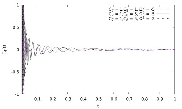
Figure 4: Plot of evolution of gravitational wave with time in a K-matter dominated spatially closed universe.

From this plot one can see that the amplitude of the wave is decaying and the frequency is also decreasing with time. A resurgence of the amplitude and frequency of the gravitational wave is not indicated in this case. This is quite expected as the universe does not re-collapse.

4 Gravitational waves in Bianchi type-I Universe

4.1 Bianchi-I metric

The observed universe, to a very high degree of accuracy ($1$ in $10^{-5}$) is isotropic. However, an anisotropic universe warrants discussion for various purposes (see the work of Rodrigues [36]). In this section, a Bianchi type-I cosmological model is taken as the background spacetime for the propagation of gravitational waves. A Bianchi type-I universe, the simplest homogeneous but anisotropic cosmological model, is described by the metric

$$ds^{2}=-dt^{2}+a^{2}(t)dx^{2}+b^{2}(t)dy^{2}+c^{2}(t)dz^{2},$$ (44)

where $a,b,c$ are functions of the cosmic time $t$. These functions can be viewed as the scale factors along the three spatial axes $x,y,z$ respectively.

4.2 Gravitational wave Equations

One can write down the non-zero components of the Christoffel symbol, Riemann tensor and Ricci tensor using the Bianchi type-I metric (44) as needed in the general gravitational wave equation (14). The individual wave equation for the $10$ components of the metric perturbation $h_{\alpha\beta}$ can be explicitly written as

$${\Box h_{00}-2\left(\left(\frac{\ddot{a}}{a^{3}}\right)h_{11}+\left(\frac{\ddot{b}}{b^{3}}\right)h_{22}+\left(\frac{\ddot{c}}{c^{3}}\right)h_{33}\right)-2\left(\frac{\ddot{a}}{a}+\frac{\ddot{b}}{b}+\frac{\ddot{c}}{c}\right)h_{00}=0,}$$ (45)

$${\Box h_{11}+2\left(\left(\frac{a\dot{a}\dot{b}}{b^{3}}\right)h_{22}+\left(\frac{a\dot{a}\dot{c}}{c^{3}}\right)h_{33}-\left(a\ddot{a}\right)h_{00}\right)-\frac{2}{a}\left(\ddot{a}+\frac{\dot{a}\dot{b}}{b}+\frac{\dot{a}\dot{c}}{c}\right)h_{11}=0,}$$ (46)

$${\Box h_{22}+2\left(\left(\frac{b\dot{a}\dot{b}}{b^{3}}\right)h_{11}+\left(\frac{b\dot{b}\dot{c}}{c^{3}}\right)h_{33}-\left(b\ddot{b}\right)h_{00}\right)-\frac{2}{b}\left(\ddot{b}+\frac{\dot{a}\dot{b}}{a}+\frac{\dot{b}\dot{c}}{c}\right)h_{22}=0,}$$ (47)

$${\Box h_{33}+2\left(\left(\frac{c\dot{a}\dot{c}}{b^{3}}\right)h_{11}+\left(\frac{c\dot{b}\dot{c}}{b^{3}}\right)h_{22}-\left(c\ddot{c}\right)h_{00}\right)-\frac{2}{c}\left(\ddot{c}+\frac{\dot{a}\dot{c}}{a}+\frac{\dot{c}\dot{b}}{b}\right)h_{33}=0,}$$ (48)

$${\Box h_{01}-2\left(\frac{\ddot{a}}{a}\right)h_{10}-\frac{1}{a}\left(\ddot{a}+\frac{\dot{a}\dot{b}}{b}+\frac{\dot{a}\dot{c}}{c}\right)h_{10}-\left(\frac{\ddot{a}}{a}+\frac{\ddot{b}}{b}+\frac{\ddot{c}}{c}\right)h_{01}=0,}$$ (49)

$${\Box h_{02}-2\left(\frac{\ddot{b}}{b}\right)h_{20}-\frac{1}{b}\left(\ddot{b}+\frac{\dot{a}\dot{b}}{a}+\frac{\dot{b}\dot{c}}{c}\right)h_{20}-\left(\frac{\ddot{a}}{a}+\frac{\ddot{b}}{b}+\frac{\ddot{c}}{c}\right)h_{02}=0,}$$ (50)

$${\Box h_{03}-2\left(\frac{\ddot{c}}{c}\right)h_{30}-\frac{1}{c}\left(\ddot{c}+\frac{\dot{c}\dot{a}}{a}+\frac{\dot{c}\dot{b}}{b}\right)h_{30}-\left(\frac{\ddot{a}}{a}+\frac{\ddot{b}}{b}+\frac{\ddot{c}}{c}\right)h_{03}=0,}$$ (51)

$${\Box h_{12}-2\left(\frac{\dot{a}}{a}\frac{\dot{b}}{b}\right)h_{21}-\frac{1}{a}\left(\ddot{a}+\frac{\dot{a}\dot{b}}{b}+\frac{\dot{a}\dot{c}}{c}\right)h_{12}-\frac{1}{b}\left(\ddot{b}+\frac{\dot{a}\dot{b}}{a}+\frac{\dot{b}\dot{c}}{c}\right)h_{21}=0,}$$ (52)

$${\Box h_{13}-2\left(\frac{\dot{a}}{a}\frac{\dot{c}}{c}\right)h_{31}-\frac{1}{a}\left(\ddot{a}+\frac{\dot{a}\dot{b}}{b}+\frac{\dot{a}\dot{c}}{c}\right)h_{13}-\frac{1}{c}\left(\ddot{c}+\frac{\dot{a}\dot{c}}{a}+\frac{\dot{b}\dot{c}}{b}\right)h_{31}=0,}$$ (53)

$${\Box h_{23}-2\left(\frac{\dot{b}}{b}\frac{\dot{c}}{c}\right)h_{32}-\frac{1}{b}\left(\ddot{b}+\frac{\dot{a}\dot{b}}{a}+\frac{\dot{b}\dot{c}}{c}\right)h_{23}-\frac{1}{c}\left(\ddot{c}+\frac{\dot{a}\dot{c}}{a}+\frac{\dot{b}\dot{c}}{b}\right)h_{32}=0}~{}.$$ (54)

Here $x^{1},x^{2},x^{3}$ correspond to $x,y,z$ respectively. One can check the consistency of these equations. In particular, by choosing the special case of $a(t)=b(t)=c(t)$, one can see that the equation system matches with that for the spatially flat FRW metric.

4.3 Solutions to the gravitational wave equations

To solve the wave equations for the anisotropic universe, we shall follow the same techniques which we have used earlier. We shall use the gauge condition to reduce the number of the independent equations. Here we choose a coordinate system, in which the wave propagates in $x$ direction. So according to TTS gauge, $h_{0\alpha}$ and $h_{1\alpha}$ (for all $\alpha$) components will be identically zero. Hence, we have only two non-zero independent components of the metric perturbations $h_{\alpha\beta}$, viz. $h_{22}$ and $h_{23}$. So, we are left with two wave equations

$${\Box h_{22}+2\left(\left(\frac{b\dot{a}\dot{b}}{b^{3}}\right)h_{11}+\left(\frac{b\dot{b}\dot{c}}{c^{3}}\right)h_{33}-\left(b\ddot{b}\right)h_{00}\right)-\frac{2}{b}\left(\ddot{b}+\frac{\dot{a}\dot{b}}{a}+\frac{\dot{b}\dot{c}}{c}\right)h_{22}=0,}$$ (55)

$${\Box h_{23}-2\left(\frac{\dot{b}}{b}\frac{\dot{c}}{c}\right)h_{32}-\frac{1}{b}\left(\ddot{b}+\frac{\dot{a}\dot{b}}{a}+\frac{\dot{b}\dot{c}}{c}\right)h_{23}-\frac{1}{c}\left(\ddot{c}+\frac{\dot{a}\dot{c}}{a}+\frac{\dot{b}\dot{c}}{b}\right)h_{32}=0,}$$ (56)

To integrate these equations, at first we shall expand the d’Alembertian. To simplify the calculations, we shall take that the perturbation components are only function of $x$ and $t$. We express two independent components of the metric perturbation as $h_{22}=\phi(t,x)$ and $h_{23}=\psi(t,x)$. The d’Alembertian simplifies to the following form,

$$\Box h_{22}=\Box\phi=-\ddot{\phi}-\left(\frac{\dot{a}}{a}+\frac{\dot{b}}{b}+\frac{\dot{c}}{c}\right)\dot{\phi}+\frac{1}{a^{2}}\phi^{{}^{\prime\prime}}~{},$$ (57)

$$\Box h_{23}=\Box\psi=-\ddot{\psi}-\left(\frac{\dot{a}}{a}+\frac{\dot{b}}{b}+\frac{\dot{c}}{c}\right)\dot{\psi}+\frac{1}{a^{2}}\psi^{{}^{\prime\prime}}~{},$$ (58)

where a dot represents the time-derivative and the prime represents the derivative with respect to $x$-coordinate. For definiteness, we consider anisotropic Kasner metric solution [34] to describe the background spacetime dynamics [35]. The Kasner metric solution is an exact solution of Einstein’s field equation and is given by

$$ds^{2}=-dt^{2}+t^{2p_{1}}dx^{2}+t^{2p_{2}}dy^{2}+t^{2p_{3}}dz^{2},$$ (59)

where constants $p_{1},p_{2},p_{3}$ are known as Kasner exponents. The Kasner metric represents a spatially flat universe but depending upon the values of $(p_{1},p_{2},p_{3})$ the universe may expand or contract at different rates in different directions. The Kasner exponents satisfy following two conditions

$$\sum_{i=1}^{3}p_{i}=1~{},~{}\sum_{i=1}^{3}p^{2}_{i}=1~{}.$$ (60)

In other words, we shall consider $a(t)=t^{p_{1}}$, $b(t)=t^{p_{2}}$ and $c(t)=t^{p_{3}}$ in the wave equations for $h_{22}$ and $h_{23}$ (Eqs. 57, 58).

4.3.1 Propagation in the plane of symmetry

Let us consider the Kasner exponents to be $(p_{1},p_{2},p_{3})$=$\left(\frac{2}{3},\frac{2}{3},-\frac{1}{3}\right)$, so that the universe is expanding at the same rate in the $x$ and $y$ directions while it is contracting in the $z$ direction. As a result, there is a plane of symmetry in the $x$-$y$ plane. We have already assumed the wave is propagating along the $x$ direction. Now using $h_{\alpha 1}=0$ and $h_{\alpha 0}=0$, for all $\alpha$, we get $h_{00}=h_{11}=0$. Also the traceless condition gives $h_{22}=-h_{33}$. We substitute $a(t)=t^{p_{1}}$, $b(t)=t^{p_{2}}$ and $c(t)=t^{p_{3}}$ with $(p_{1},p_{2},p_{3})=\left(\frac{2}{3},\frac{2}{3},-\frac{1}{3}\right)$ in the wave equation for $h_{22}=\phi(t,x)$. The wave equation for $\phi$ then becomes

$$\Box\phi+\left(\frac{4}{9}\right)\phi=0~{},$$ (61)

which yields

$$\ddot{\phi}+\left(\frac{1}{t}\right)\dot{\phi}-\left(\frac{1}{t^{\frac{4}{3}}}\right)\phi^{{}^{\prime\prime}}-\left(\frac{4}{9}\right)\phi=0~{}.$$ (62)

By considering $\phi(t,x)=X_{5}(x)T_{5}(t)$, the $x$-dependent differential equation becomes

$$X_{5}^{{}^{\prime\prime}}+{\Omega}^{2}X_{5}=0~{},$$ (63)

where ${\Omega}^{2}$ is the separation constant. The solution is simple,

$$X_{5}(x)=A\cos({\Omega}x)+B\sin({\Omega}x),$$ (64)

where $A$ and $B$ are constants of integration. The temporal part of the differential equation is given by

$$\ddot{T_{5}}+\left(\frac{1}{t}\right)\dot{T_{5}}-\left(\frac{4}{9}-\frac{{\Omega}^{2}}{t^{\frac{4}{3}}}\right)T_{5}=0~{}.$$ (65)

It appears that the equation (65) is not known to have any analytic solution.

On the other hand, the wave equation for $h_{23}=\psi(t,x)$ component can be expressed as

$$\Box\psi+\left(\frac{4}{9t^{2}}\right)\psi=0~{},$$ (66)

which leads to

$$\ddot{\psi}+\left(\frac{1}{t}\right)\dot{\psi}-\left(\frac{1}{t^{\frac{4}{3}}}\right)\psi^{{}^{\prime\prime}}-\left(\frac{4}{9t^{2}}\right)\psi=0~{}.$$ (67)

We consider $\psi(t,x)=X_{6}(x)T_{6}(t)$. As earlier, the $x$-dependent differential equations becomes

$$X_{6}^{{}^{\prime\prime}}+{\Omega}^{2}X_{6}=0~{},$$ (68)

which has the solution $X_{6}(x)=C\cos({\Omega}x)+D\sin({\Omega}x)$, with $C$ and $D$ being constants of integration. The temporal part of differential equations is given by

$$\ddot{T_{6}}+\left(\frac{1}{t}\right)\dot{T_{6}}-\left(\frac{4}{9t^{2}}-\frac{{\Omega}^{2}}{t^{\frac{4}{3}}}\right)T_{6}=0~{}.$$ (69)

The analytical solution to the equation (69) is given by

$$T_{6}(t)=C_{9}J_{2}\left(3{\Omega}t^{\frac{1}{3}}\right)+C_{10}Y_{2}\left(3{\Omega}t^{\frac{1}{3}}\right)~{},$$ (70)

where $C_{9}$, $C_{10}$ are the constants of integration. Here $J_{n}(z)$, $Y_{n}(z)$ are the Bessel functions of the first kind and the second kind respectively. The parameter $n$ refers to the order of the Bessel functions.

We plot $T_{6}$ for various combinations of the constants of integration and the constant of separation in the FIG. 5. We can clearly see from the plot that the frequency and amplitude are decreasing with time. The rate of diminution is different for the different cases. The amplitude is scaled by its initial value and the unit of time is $H_{0}^{-1}$ as $p_{1}+p_{2}+p_{3}=1$ where $H=\frac{1}{3}(H_{1}+H_{2}+H_{3})$. Here $H_{i}$ is the Hubble expansion rate along the $i$th spatial direction, e.g., $H_{1}=\frac{\dot{a}}{a}$ and so on. The suffix $0$ indicates the value of the quantity at $a=b=c=1$ in the present context of scaling.

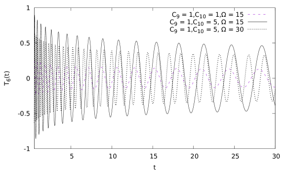
Figure 5: Plot of evolution of gravitational wave with time in Kasner metric where plane of symmetry is in the $x$-$y$ plane.

4.3.2 Propagation along the normal to the plane of symmetry

In this case, we consider the gravitational wave to be propagating along the normal to the plane of symmetry. Let us consider $(p_{1},p_{2},p_{3})$=$\left(-\frac{1}{3},\frac{2}{3},\frac{2}{3}\right)$, so that the universe is expanding at the same rate in $y$ and $z$ directions while contracting in $x$ direction. Therefore, there is a plane of symmetry in the $y$-$z$ plane and since the gravitational wave is propagating in the $x$-direction, this case corresponds to the wave propagating normal to this plane. Here again we choose $h_{00}=h_{11}=0$ and the traceless condition gives $h_{22}=-h_{33}$. We substitute $a(t)=t^{p_{1}}$, $b(t)=t^{p_{2}}$ and $c(t)=t^{p_{3}}$ with the chosen Kasner exponents in the wave equation. In this case of gravitational wave propagating along the normal to the plane of symmetry, the differential equations for $h_{22}=\phi(t,x)$ and $h_{23}=\psi(t,x)$ are exactly same and given by

$$\ddot{\psi}+\left(\frac{1}{t}\right)\dot{\psi}-\left(\frac{1}{t^{-{\frac{2}{3}}}}\right)\psi^{{}^{\prime\prime}}+\left(\frac{8}{9t^{2}}\right)\psi=0.$$ (71)

Using separation of variables, we consider $\psi(t,x)=X_{7}(x)T_{7}(t)$, which yields the $x$-dependent differential equation as $X_{7}^{{}^{\prime\prime}}+{\Omega}^{2}X_{7}=0,$ where ${\Omega}^{2}$ is the separation constant. The corresponding solution is $X_{7}(x)=G\cos({\Omega}x)+H\sin({\Omega}x)$ where $G$ and $H$ are constants of integration. The $t$-dependent differential equation is given by

$$\ddot{T_{7}}+\left(\frac{1}{t}\right)\dot{T_{7}}+\left(\frac{8}{9t^{2}}+{\Omega}^{2}t^{\frac{2}{3}}\right)T_{7}=0~{},$$ (72)

which has an analytical solution of the form

$$T_{7}(t)=J_{-\frac{i}{\sqrt{2}}}\left(\frac{3}{4}\Omega t^{\frac{4}{3}}\right)\Gamma\left(1-\frac{i}{\sqrt{2}}\right)C_{11}$$

$$+J_{\frac{i}{\sqrt{2}}}\left(\frac{3}{4}\Omega t^{\frac{4}{3}}\right)\Gamma\left(1+\frac{i}{\sqrt{2}}\right)C_{12}~{}.$$ (73)

Here, $C_{11}$, $C_{12}$ are constants of integration. $J_{n}(z)$ is the Bessel function of first kind where $n$ is its order and $\Gamma(z)$ is the Gamma function with argument $z$.

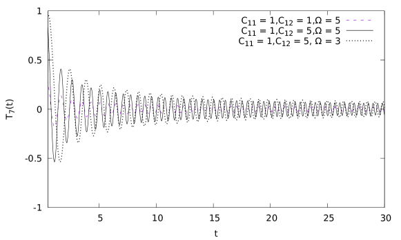
Figure 6: Plot of evolution of gravitational wave with time in Kasner metric where plane of symmetry is $y$-$z$ plane.

For various choices of the constants, the plot for $T_{7}(t)$ is given in the FIG. 6. As in the previous case, the frequency and amplitude both are decreasing with time.

5 Discussion

In this work we present exact solutions of the equation for the gravitational waves in some cosmological backgrounds in the linear regime of the perturbation where the nonlinear contributions from the perturbations are not considered. This linearized wave equation is solved for the dust dominated and also the radiation dominated spatially flat isotropic universe. As already mentioned in section 2, we worked in a short wave condition. The idea was not to look at the full spectrum of the gravity wave. The interest clearly was to see how the amplitude and frequency of the wave are modified in the cosmologial background. Qualitatively, other modes, if any, should also undergo similar changes. Both the amplitude and frequency are found to decay with time (figures 1 and 2). For a spatially closed universe, the exact solutions are obtained for two cases. For a standard radiation dominated universe, the amplitude and frequency decrease to start with, but after reaching a minimum, increases at the same rate (figure 3). This apparently intriguing feature is actually quite consistent, as the universe recollapses, after reaching a maximum volume, into a big crunch in this model. The other example for the closed universe is for the so-called K-matter distribution ($P=-\frac{1}{3}\rho$) which gives Milne’s “coasting” universe which expands with a zero deceleration parameter $q$. The amplitude and frequency both monotonically decay as given in figure 4. The temporal parts of the two degrees of freedom (or the two modes) of the gravitational wave have the same equation for any given isotropic model.

For the anisotropic case, we take up the Kasner metric as the example with a plane of symmetry. If the wave propagates in the plane of symmetry, the two modes have different equations for the temporal part. For one mode ($h_{23}=h_{32}$) the exact solution is obtained, whereas for the other ($h_{22}=-h_{33}$) we failed to get an analytic solution. For the wave propagating normal to the plane of symmetry, the two modes behaves identically, and the exact solution is indeed obtained. The wave form for the exactly solved cases are given in figures 5 and 6. The behaviour is similar to the isotropic expansion, a monotonic decay of both the amplitude and frequency.

As already mentioned, the exact numerical values for the initial conditions that fixes the constants of integration, or the exact values of other constants (such as the constant of separation) are not rigorously settled in any way for the present work. The focus is more on the exact solutions of the wave equations, and it is clearly demonstrated that they can be written, at least in some special cases. The examples of the cosmologies chosen are not contrived, they are there in the literature and are quite widely used. The time axis in the plots are scaled not to any standard unit, but it does not obscure the nature of the plots in any way. Each of the plots is a family of curves, where each member represents a set of constants. It is quite apparent from all the figures that the nature of the evolution is not too sensitive to the choice of the constants.

References

- [1] R. A. Hulse and J. H. Taylor, Astrophys. J. 195, L51 (1975).
- [2] B. P. Abbott et al. [LIGO Scientific and Virgo Collaborations], Phys. Rev. Lett. 116, no. 6, 061102 (2016).
- [3] B. P. Abbott et al. [LIGO Scientific and Virgo Collaborations], Phys. Rev. Lett. 116, no. 24, 241103 (2016).
- [4] B. P. Abbott et al. [LIGO Scientific and Virgo Collaborations], Phys. Rev. Lett. 119, no. 14, 141101 (2017).
- [5] B. P. Abbott et al. [LIGO Scientific and Virgo Collaborations], Phys. Rev. Lett. 119, no. 16, 161101 (2017)
- [6] W. M. Farr, M. Fishbach, J. Ye and D. Holz, Astrophys. J. Lett. 883, L42 (2019).
- [7] B.P. Abbott et al [LIGO Scientific and Virgo Collaborations], Phys. Rev X, 9, 031040 (2019).
- [8] R. A. Isaacson, Phys. Rev. 166, 1263 (1968).
- [9] L. E. Mendes and A. R. Liddle, Phys. Rev. D, 60, 063508 (1999).
- [10] N. Seto and J. Yokoyama, J. Phys. Soc. Jap., 72, 3082 (2003).
- [11] S. Kuroyanagi, T. Takahashi and S. Yokoyama, JCAP, 1502, 003 (2015).
- [12] S. Capozziello, M. DeLaurentis and M. Francaviglia, Astropart. Phys., 29, 125 (2008).
- [13] P. Valtancoli, Annals Phys. 394, 225 (2018).
- [14] W. Kulczycki and E. Malec Phys. Rev. D, 96, 063523 (2017).
- [15] P. Creminelli and F. Vernizzi Phys. Rev. Lett, 119, 1302 (2017).
- [16] J.B. Jimenez and L. Heisenberg JCAP, 1807, 035 (2018)
- [17] R.R. Caldwell and C. Devulder Phys. Rev. D, 100, 103510 (2019)
- [18] M. Bradley, M. Forsberg and Z. Keresztes Universe, 3, 49 (2017).
- [19] O. Dunya and M. Arik Gen. Rel. Grav., 51, 94 (2019).
- [20] R.C. Nunes, S. Pan and E.N. Saridakis Phys. Rev. D, 98, 104055 (2018)
- [21] R.C. Nunes, M.E.S. Alves and J.C.N. deAraujo Phys. Rev. D, 99, 084022 (2019).
- [22] S. Capozziello, M. DeLaurentis, S. Nojiri and S.D. Odintsov Phys. Rev. D, 95, 083524 (2017)
- [23] R. Flauger and S. Weinberg, Phys. Rev. D 97, 123506 (2018)
- [24] T. Padmanabhan, Gravitation: Foundations and Frontiers, Cambridge, UK: Cambridge Univ. Pr. (2010) 700 p
- [25] O. Svitek and J. Podolsky, Czech. J. Phys. 56, 1367 (2006)
- [26] L. H. Ford and L. Parker, Phys. Rev. D 16, 1601 (1977).
- [27] M. Maggiore, Gravitational Waves. Vol. 1: Theory and Experiments, Oxford University Press (2007)
- [28] L. P. Grishchuk and A. D. Popova, Sov. Phys. JETP 53, 1 (1981).
- [29] R. R. Caldwell, Phys. Rev. D 48, 4688 (1993).
- [30] E. W. Kolb, Astrophys. J. 344, 543 (1989).
- [31] M. Gasperini, Elements of string cosmology, Cambridge University Press, 2007.
- [32] P. D. D’Eath, Annals Phys. 98, 237 (1976).
- [33] J. Bicak and J. B. Griffiths, Annals Phys. 252, 180 (1996).
- [34] E. Kasner, Am. J. Math. 43, 217 (1921).
- [35] B. L. Hu, Phys. Rev. D 18, 969 (1978).
- [36] D.C. Rodrigues, Rev. D, 77, 023534 (2008).