A posteriori error estimation for the non-self-consistent Kohn-Sham equations
Abstract
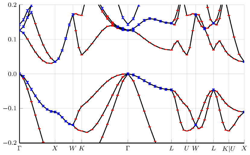
We address the problem of bounding rigorously the errors in the numerical solution of the Kohn-Sham equations due to (i) the finiteness of the basis set, (ii) the convergence thresholds in iterative procedures, (iii) the propagation of rounding errors in floating-point arithmetic. In this contribution, we compute fully-guaranteed bounds on the solution of the non-self-consistent equations in the pseudopotential approximation in a plane-wave basis set. We demonstrate our methodology by providing band structure diagrams of silicon annotated with error bars indicating the combined error.
I Introduction
Experimental results are provided with error bars in most scientific fields. In an ideal world, this should also be the case for results obtained by numerical simulation. Complementing simulation results with error bars is becoming mandatory in some branches of engineering, such as aeronautics or car industry, in which simulation has partially, or even totally, replaced experiment (e.g. virtual wind tunnels Mo et al. (2013) or crash simulators Spethmann et al. (2009)). Obviously, uncontrolled errors in the numerical simulations used to design and test an aircraft are likely to have dramatic consequences for passengers and crews.
What about molecular simulation? Statistical error bars are often displayed in molecular dynamics (MD) and quantum Monte Carlo (QMC), where stochastic processes (e.g. Langevin equation for MD, drift-diffusion stochastic differential equations for QMC) are at the core of the simulation. However, these error bars are purely statistical in nature and are not guaranteed: they only reflect the finiteness of the statistical sample and the actual solution of the model has a positive probability to lay outside the confidence interval. In addition, they only take into account one of the components of the error between the exact value of the quantity of interest (q.o.i.) and its numerical approximation. The other components of the error are deterministic in nature and are also present in simulations of purely deterministic models, such as those based on density-functional theory (DFT) which are dealt with in the article.
Consider as an example of q.o.i. the lattice constant of Silicon at 0 K. In order to compute a numerical approximation of this q.o.i., we first have to select a model. We have at our disposal an outstanding model: the many-body Schrödinger equation with relativistic corrections. However, solving this equation directly is completely out of reach. The first approximation is to replace this reference model with a cruder, but tractable, reduced model. We consider as a reduced model the one obtained by successively using the Born-Oppenheimer approximation to decouple as much as possible nuclear and electronic degrees of freedom, and the Local Density Approximation of the Kohn-Sham density-functional theory (KS-LDA), together with a pseudopotential model to avoid representing core electrons and the singularities of the orbitals near atoms. This gives rise to a well-defined mathematical model, hopefully with a unique solution. We refer to the difference between this approximation and the physical reality as the model error.
The reduced model, though simpler than the reference model, still has an infinite number of degrees of freedom, and must be discretized to be simulated. For the crystalline phase, a typical (simplified) workflow is as follows Martin and Martin (2004):
-
1.
The infinite computational domain is truncated to a finite supercell with periodic boundary conditions, numerically handled through Brillouin zone sampling;
-
2.
In this supercell, crystalline orbitals are discretized using a finite basis set of plane waves;
-
3.
The self-consistent Kohn-Sham equations are solved by a self-consistent field (SCF) algorithm;
-
4.
At each step of the SCF algorithm, a linear eigenvalue equation is solved with an iterative eigensolver;
-
5.
All computations are performed with finite precision.
We refer to the error in steps 1 and 2 as the discretization error, to the error in steps 3 and 4 as the algorithmic error, and to the error in step 5 as the arithmetic error. To these must be added programming errors, not to be neglected in codebases consisting of millions of lines of code, and hardware errors, which are expected to become significant for exascale architectures Snir et al. (2014). These two latter kinds of errors we will not treat.
Note that all steps mentioned above are systematically improvable: by increasing parameters, such as Brillouin zone sampling, basis set cutoff, convergence thresholds, or using higher-precision arithmetic, results get more accurate at the price of longer computation times. The usual procedure for controlling these errors is to perform convergence studies: on the system of interest or a related system with similar characteristics, the parameter is increased until the variation of the quantity of interest is below a specified tolerance. Over time, knowledge of “good” parameter values solidifies into rules of thumb that are automated in codes or suggested to users in manuals. When used appropriately, this results in acceptable errors that are below the target accuracy (for instance, for pseudopotential methods, the error compared to all-electron models) Lejaeghere et al. (2014, 2016).
This empirical process is however still problematic. First, it might result in suboptimal performance by excess of caution. Second, it still requires a degree of hand-tuning and is thus problematic for fully automated computations, which are useful for in silico design of novel compounds and for building databases of material or chemical properties. Third, the rules of thumb can fail for unusual systems with unexpected behavior, i.e. exactly those where accurate simulations are important to aid understanding.
The purpose of a posteriori error analysis is to automate and rationalize this process by providing accurate, computable and guaranteed bounds on the error of each step. The purpose of this is twofold. First, bounds of the total error on the q.o.i. can be obtained by simply summing up the different components of the error, allowing one to bound the accuracy of the final result. Second, the computer resources necessary to reach a given accuracy on the final result can be optimized by error balancing techniques. For instance, convergence thresholds should be adapted to the discretization: if the discretization is coarse, it is not necessary to use extremely tight convergence criteria, since the final accuracy will be limited by the discretization error anyway. For the same reason, it might suffice to perform most operations in single-precision arithmetic to save computational time without losing much on the accuracy of the final result. Error balancing based on a posteriori error bounds allows one to turn these common sense remarks into black-box numerical strategies. The user provides the target accuracy and the software automatically chooses, in an adaptive way along the iterative process, the reduced models, discretization bases, convergence thresholds, and data structures to obtain the desired accuracy at a quasi-optimal computational cost.
Applying this methodology to electronic structure calculations is a challenge due to the complexity of the equations. Despite this, significant progress has been made in the past decade towards rigorous error control, which makes this perspective realistic in the medium term. Let us mention in particular recent works on a priori and a posteriori discretization error bounds for DFT Cancès et al. (2012); Chen et al. (2013); Chen and Schneider (2015a, b); Kaye et al. (2015); Cancès et al. (2016, ressa), including -point sampling Cancès et al. (ressb), and on the numerical analysis of SCF algorithms Chupin et al. (2020); Dai et al. (2017); Rohwedder and Schneider (2011); Zhao et al. (2015).
In this contribution, we provide for the first time a combined analysis of the errors in step 2 (basis set truncation), 4 (inexact solution of the eigenvalue problem) and 5 (arithmetic error). The q.o.i. is the band diagram of silicon, or more precisely the energies of the 3 highest occupied and 4 lowest unoccupied crystalline orbitals for specific -points. The models under consideration are the Cohen-Bergstresser model Cohen and Bergstresser (1966) on the one-hand, and the non-self-consistent (electron-electron interaction completely neglected) periodic KS-LDA model with GTH pseudopotentials Goedecker et al. (1996); Hartwigsen et al. (1998) on the other hand, for which we will give fully guaranteed error bounds.
Some aspects of our analysis, such as the computation of the residual, are general and can be extended to other quantities of interest, basis sets and models; others, such as the gap estimation, rely more specifically on properties of the setup considered. We refer to the conclusion for more details on this point. Our analysis is, however, limited in its present state due to the neglect of the errors in steps 1 (Brillouin zone sampling) and 3 (self-consistency). We hope to address both these challenging aspects in future publications.
Let us finally point out that the model error arising from the choice of density-functional theory is not easily systematically improvable. For wavefunctions methods (e.g. coupled-cluster methods Rohwedder and Schneider (2013)) guaranteed a posteriori error bounds on the model error — with respect to the many-body Schrödinger equation (MBSE) — can in principle be derived, since a residual of the MBSE can be computed from the approximate wavefunction and energy. For DFT, on the other hand, this is not easily the case such that guaranteed model errors are probably out of reach and going beyond machine-learned confidence intervals obtained from big data sets of reference calculations seems very difficult. Regarding pseudopotentials and related approaches, the Projector Augmented Wave Blöchl (1994) (PAW) method should be amenable to the derivation of guaranteed error bounds - with respect to reference full-electron DFT calculations - since approximate all-electron Kohn-Sham orbitals can be reconstructed from PAW pseudo-orbitals allowing the construction of a residual.
II Kohn-Sham density-functional theory in the pseudopotential approximation
As already mentioned in the introduction, the q.o.i. under consideration are the energies of crystalline orbitals at specific -points, in a non-self-consistent pseudopotential model. In the following we denote by the periodic lattice, and assume that the Bloch wavevector is fixed in the Brillouin zone. The equation we solve is
| (1) |
with an -periodic function and the unit cell. The periodic Hamiltonian is given by
where the (possibly nonlocal) effective potential is assumed to be known.
The problem (1) is discretized in a Fourier basis: any -periodic function can be expanded on the orthonormal plane-wave basis
where is the volume of the unit cell, and belongs to the reciprocal lattice . The complete set is truncated to obtain a finite approximation space
with dimension , for some finite cutoff energy . We will use the convenient abuse of notation consisting in writing to denote a such that . The linear eigenvalue equation (1) is then discretized by invoking the variational principle: the complex Hermitian matrix
is diagonalized using an iterative eigensolver Saad (2011); Kresse and Furthmüller (1996), employing fast Fourier transform to perform matrix-vector products efficiently.
The potential can be a purely local potential, or have a nonlocal component in the case of norm-conserving pseudopotentials. We will consider two cases here, chosen for their simple analytic forms.
First we consider the Cohen-Bergstresser pseudopotentials for semiconductors in the diamond and zinc-blende structure Cohen and Bergstresser (1966). These are extremely purely local -periodic potentials with a small number of non-zero Fourier coefficients. More precisely
| (2) |
where is only nonzero for in a small finite set (the first five shells of reciprocal vectors). The coefficients were adjusted to reproduce spectroscopic data.
We next consider more realistic Goedecker–Teter–Hutter (GTH) norm-conserving potentials Goedecker et al. (1996); Hartwigsen et al. (1998). These potentials are composed of a local and a non-local part:
where
| (3) |
Here runs over all the atoms in the unit cell, the range of angular momentum depends on the chemical element considered, and the projection indices are summed over a small number of integers (two in the case of silicon). The coefficients are finite sums of products of three terms: a structure phase factor depending on the position of the atoms in the unit cell, a radial Gaussian envelope and a radial rational function. The are the product of a structure phase factor, a spherical harmonics , a radial Gaussian envelope and a radial polynomial of degree . Among the many types of pseudopotentials available, we chose this type because their analytic form (rather than tabulated data) lends itself well to rigorous error analysis.
All computations presented in this paper have been performed using the density-functional toolkit (DFTK) Herbst and Levitt , a recent Julia Bezanson et al. (2017) implementation for Kohn-Sham DFT and related methods using plane-wave basis sets. Our implementation of the discussed estimates and the code producing the figures of this paper is available on Github Herbst et al. .
III From residuals to errors
Assume for simplicity that is an isolated eigenvalue of . Given a finite , the result of the iterative procedure is a normalized vector and a Riesz approximation of the eigenvalue , such that the algebraic residual , where is the orthogonal projector on , is small. Note that the algebraic residual vanishes for an exact matrix eigensolver, in contrast with the global residual , which is always nonzero due to the finite basis discretization. The question we are interested in is: can we bound rigorously the error between and ?
Several a posteriori error bounds for elliptic eigenvalue problems are available in the literature Goerisch and He (1990); Babuška and Osborn (1991); Heuveline and Rannacher (2001); Mehrmann and Miedlar (2011); Kuznetsov and Repin (2013); Bank et al. (2013); Carstensen and Gedicke (2014); Liu (2015); Cancès et al. (2018), the most accurate of them requiring lower bounds on the distance between the eigenvalue or cluster of eigenvaluesGallistl (2014, 2015); Dai et al. (2015); Bonito and Demlow (2016); Boffi et al. (2017); Cancès et al. (ressa) of interest and the rest of the spectrum. We focus here on two basic bounds for the sake of simplicity: the implementation of more accurate ones is work in progress.
Theorem 1 (Bauer-Fike).
There exists an eigenvalue of such that
This bound is very easy to handle: it only requires an upper bound on the -norm of the residual. It is however not sharp. In particular, it is well-known that the error on isolated eigenvalues of Hermitian matrices behaves as the square of the residual. An a posteriori error bound having this property is the following.
Theorem 2 (Kato-Temple).
Let be the eigenvalue of closest to . Assume that is an isolated point of the spectrum of with a distance to the rest of the spectrum. Then
| (4) |
The proof of both these theorems can be found in standard textbooks Saad (2011).
To apply these bounds, we need three ingredients: (i) construct an upper bound on the residual , (ii) construct a lower bound on the gap , (iii) implement these bounds in the presence of roundoff errors. We address these problems in sequence.
IV Computing the residual
Assuming that the variational numerical method provides an approximate normalized eigenfunction
with
and a Riesz approximation of the associated eigenvalue, then the square norm of the residual
can be decomposed as
| (5) | ||||
where and are the orthogonal projectors on and respectively. Here we have used that the kinetic energy operator is diagonal in reciprocal space, so that . The first term, which is easily computed in the Fourier basis of , is the square of the norm of the in-space, algebraic residual . It is driven to zero by the iterative eigensolver but does not vanish because the iterations stop when the convergence thresholds are reached. This is the origin of the algorithmic error, and is easily computed explicitly. The second term is the out-of-space residual and is the source of the discretization error. This term is more difficult to compute, and most often in practice only an upper bound can be obtained at a reasonable computational cost.
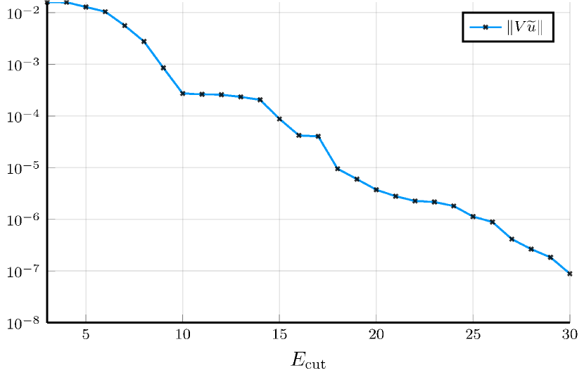
IV.1 Cohen-Bergstresser model
In this model, is given by (2), and only a small number of terms are non-zero. In this case
This computation extends over a finite range of . Denoting by the norm of the largest non-zero Fourier mode of , these can be identified to be of the form for and . It follows that belongs to the finite-dimensional space
| (6) |
with . We therefore extend to this new basis by zero-padding, and compute in this new basis, resulting in an exact computation of the residual. The very quick decay of the residual with increasing is shown in Figure 1 for the first eigenvalue at the point.
IV.2 Goedecker–Teter–Hutter (GTH) pseudopotentials
With the GTH pseudopotentials, extends on all wave vectors in , and therefore we cannot compute explicitly. Rather, as before, we compute , where the larger approximation subspace , still defined by (6) is determined by a chosen . We then bound the remaining term
We do this by exploiting the fact that the matrix elements connecting small wave vectors in to large wave vectors in are small. We obtain an explicit bound using our knowledge of and the decay properties of Gaussians, see Appendix A for details.
Our rigorous bound of the residual is plotted Figure 2 along with its different components as a function of , for an initial obtained with .
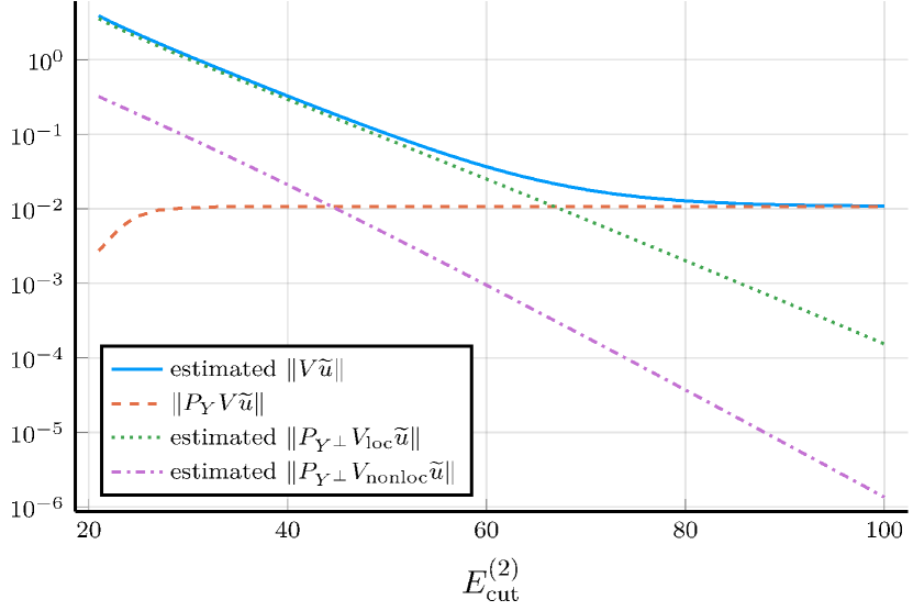
As can be seen clearly, the residual is essentially in as soon as , our estimate, however, is only accurate for larger values of . This is since our bounds for are still rather crude (see Appendix A). Improving these is work in progress.
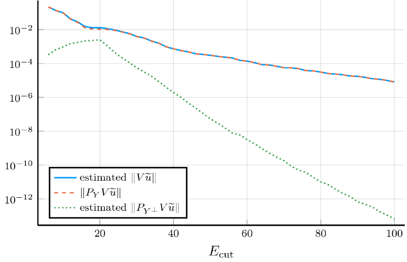
In theory, one could choose dynamically based on the size of the estimated residual. In the following, we use the simple heuristic , deduced from and Figure 2. As can be seen in Figure 3, represented the worst case for our heuristic. With this choice of the component on of the residual is negligible for all values of and our bound is nearly optimal.
V Estimating the gap
The Kato-Temple bound (4) requires a lower bound on the gap between the (unknown) exact eigenvalue and the rest of the (unknown) spectrum of . Let be the index of the target eigenvalue. Given an operator with eigenvalues , how can we obtain a lower bound on both in the one direction and on in the other? In the rest of this section we focus on a lower bound for , the other one being obtained similarly.
Assume that we have computed the discretization of the Hamiltonian on a plane-wave basis set with finite cutoff energy , and let be its eigenvalues with corresponding orthonormal eigenvectors . Note that for the purposes of this section we assume that all computations inside the basis set are exact: we form explicitly the matrix representation of and diagonalize it using a dense eigensolver, and do not consider any arithmetic error.
From the variational principle, . We now need to obtain a rigorous lower bound on , which is is much more complex. Simply taking the difference may lead to an overestimation of the gap, see for example in Figure 4. To compute a proper lower bound on we express the operator on and its orthogonal complement as
In this we have used that the kinetic energy term is diagonal in a plane-wave basis and does not appear in the off-diagonal blocks. We then use the Haynsworth inertia additivity formula Haynsworth (1968): for any real threshold not in the spectrum of , the number of eigenvalues of below is equal to the number of negative eigenvalues of the block plus the number of negative eigenvalues of the Schur complement
For pedagogical purposes we briefly sketch the proof of this statement in the simplified case where is positive. Consider the quadratic form
where . For a fixed , this is again a quadratic form in , which can be explicitly minimized by solving a linear system:
and therefore
It follows that is positive if and only if is. The extension to arbitrary number of negative eigenvalues proceeds similarly.
From this, it follows that if we manage to prove that is positive for some , we obtain that . Assume that we have computed eigenvectors up until index . Then the Schur complement can be bounded from below by expanding on its eigenvector basis
| (7) | ||||
where is the operator norm on the space of bounded linear operators on . Computing the term requires knowing the potential on all of the complement , which is not feasible for GTH pseudopotentials. Similarly as with the residuals, we assume that we are able to compute on a superset and additionally able to bound it on . With this in place we split into contributions inside and outside of :
| (8) | ||||
where is the diagonal matrix of eigenvalues and the orthogonal matrix of corresponding eigenvectors (column-wise).
To compute the first term we use the fact that is a computable, long-and-thin matrix (more rows than columns). We can employ the decomposition to factorize it into the product of an orthogonal matrix and a (small) triangular matrix . The first term in the right-hand side of (8) can then be explicitly computed as the largest eigenvalue of the (small) Hermitian matrix . The second term can be treated similarly. Details on our bounds on the operator norms , and for the Cohen-Bergstresser and the GTH pseudopotential models are given in Appendix A.
For a fixed , is positive for all large enough. For a given and , we find the best lower bound to , denoted by , as the maximum , for which we can ensure that is positive. This is done using a bisection algorithm on our bound of .
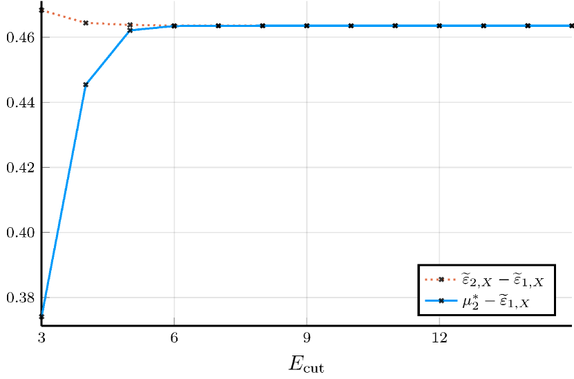
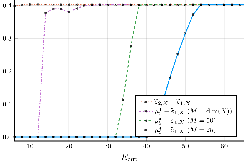
Figures 4 and 5 show gaps obtained using this lower bound on for different values of and for the first eigenvalue at the point of the two pseudopotential models we consider. For the simple Cohen-Bergstresser model and using our lower bound for the gap is accurate already at . For the GTH pseudopotentials one needs to use larger values of and .
VI Estimating the arithmetic error
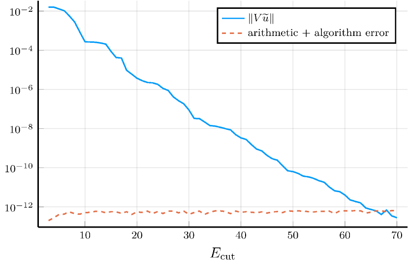
To rigorously bound the arithmetic error, we use interval arithmetic, as specified in the IEEE standard 1788-2015 IEE (2018). The main idea of interval arithmetic is to use not one but two floating-point numbers to represent a given quantity, forming an interval which contains the exact number. Every operation is then performed on the limits of the interval utilizing rounding modes of CPUs to ensure that the upper limit is only rounded upwards and the lower limit only rounded downwards if rounding is needed to represent the outcome of the operation. This ensures that the exact answer always lies between the limits of the final interval. This simplistic approach generally overestimates floating-point error, since it considers all floating-point operations independent from each other. The bound obtained in this way is thus too large making an application of interval arithmetic to, e.g. a complete iterative diagonalization algorithm, impractical. Fortunately if we obtain an approximate eigenpair inside a discretization basis using ordinary floating-point arithmetic, we only need to re-evaluate the residual norm in interval arithmetic to obtain a rigorous bound. The upper bound of the resulting interval gives access to the sum of both floating-point error and algorithmic error due to the eigensolver.
In Julia IEEE interval arithmetic is available in the IntervalArithmetic.jl Sanders et al. (2020) package as a custom floating-point type. This type can be directly used with any native Julia code, including GenericLinearAlgebra.jl Noack et al. and FourierTransforms.jl Johnson et al. , which provide interval-arithmetic equivalents to classical linear algebra and FFT algorithms. These packages allowed us to use the routines of DFTK to also bound the arithmetic error for all our double-precision calculations presented in this paper. Example values are shown in Figure 6 indicating that the obtained arithmetic error is several orders of magnitude smaller than the discretization error until around . Increasing the accuracy of the obtained solution to the Cohen-Bergstresser model beyond this point would not only require to increase the basis, but also to switch to a more accurate floating-point arithmetic beyond IEEE double precision. In a type-generic Julia code like DFTK this is, however, completely seamless and has been used to obtain Figure 7, demonstrating errors below double precision.
VII Tracking errors in band computations
With the discussed methodologies we are able to
-
•
compute the norm of the in-space residual norm (leading to the algorithmic error);
-
•
compute a guaranteed upper bound of the out-of-space residual norm (leading to the discretization error);
-
•
compute a guaranteed lower bound of the spectral gap involved in the Kato-Temple inequality (4);
-
•
compute a posteriori errors bounds on the quantities of interest (crystalline orbital energies) using either Bauer-Fike or Kato-Temple inequalities;
-
•
estimate the impact of floating-point errors via interval arithmetic (arithmetic error).
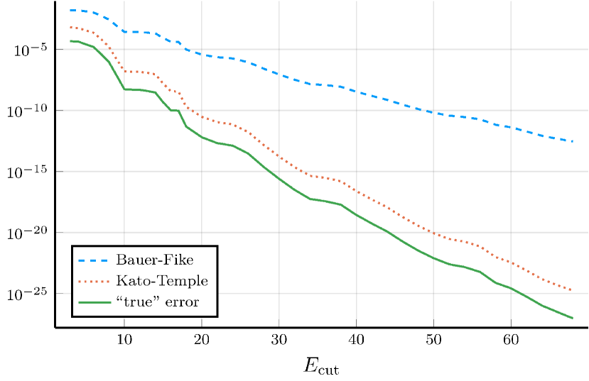
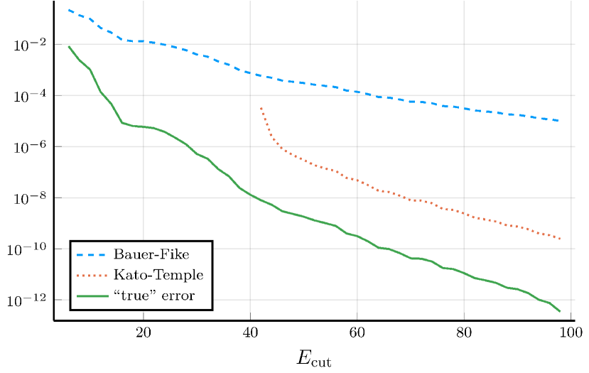
A summary of the overall numerical error on the quantities of interest bound by Bauer-Fike and Kato-Temple versus the “true” error estimated using the largest basis employed ( and respectively) is given in Figures 7 and 8 for the Cohen-Bergstresser and GTH models of silicon. Using our methods we were able to compute band structures for both models with fully guaranteed bounds on the numerical error, see Figures 9 and 10, respectively. Notice that neither Kato-Temple nor Bauer-Fike universally provide the best bound on the error, with the Kato-Temple bound being inapplicable for degenerate eigenvalues in particular. In our plots we alternate between both bounds, only showing the one providing the smallest error. The design and use of error bounds robust to degenerate eigenvalues is left to future work.
VIII Conclusions and outlook
We have discussed the computation of fully guaranteed bounds to the error in the numerical solution of non-self-consistent Kohn-Sham equations. While many other sources of error exist, our treatment focused exclusively on the discretization error, due to finite basis sets, algorithm error, due to non-zero convergence thresholds, and arithmetic error, due to finite-precision floating-point arithmetic. As quantities of interest we considered the band energies around the Fermi level of the Cohen-Bergstresser and GTH pseudopotential models and demonstrated the feasibility of our approach by providing, for each model, band structure diagrams of silicon, in which the total numerical error was annotated in the form of error bars. In this paper we have focused on error bounds on eigenvalues for simplicity, but that is not a major limitation of our approach; error bounds on eigenvectors can be obtained in a similar fashion to the Kato-Temple bound (see Saad (2011), Theorem 3.9). From there it is possible to obtain bounds on other quantities of interest, for instance the density or the forces.
Our presented approach relies on two key ingredients. First, a bound on the residual, including both its in-space component (the one driven to zero by the iterative solvers) and its out-of-space component. For the out-of-space component, we relied in this work on the properties of plane-wave basis and of the analytical pseudopotential; however, this can in principle be applied to any basis set for which exact analytical computations are possible, such as Gaussian basis sets. The second ingredient is to relate the residual to the actual error, which involved for our particular quantities of interest an eigenvalue gap. This is much more complex to perform in full rigor, as it requires a control of the out-of-basis part of the full operator itself. Achieving a similar analysis to ours in Gaussian basis sets (for instance) is a major research challenge.
A limitation of our study is that we only considered non-self-consistent models. Taking into account self-consistency in error bounds one runs into two separate issues. First, the non-convexity of the model due to the exchange-correlation term can introduce multiple energy local minima, and it is impossible to certify that the true ground state has been found. One then has to settle for a less ambitious notion of error control: showing that there exists a solution of the equation close to the numerically obtained approximate solution. Second, rigorously proving error bounds for nonlinear problems involves mathematically more sophisticated techniques to achieve a sufficient control on the nonlinear terms. This has been performed for the Gross-Pitaevskii equation, an equation similar in form but simpler than Kohn-Sham DFT Dusson and Maday (2017). Extending this to Kohn-Sham DFT is work in progress.
Finally, we hope to use our bounds to enable a fully black-box modeling, where accuracy parameters such as the kinetic energy cutoff, the convergence thresholds of the iterative solver or employed floating-point precision are chosen automatically by the code. The hope is to be able to dynamically adjust such accuracy parameters during a simulation to do as little work as necessary to reach the accuracy desired by the user. For such purposes we expect the presented Kato-Temple-type bounds to be not tight enough, so that better bounds have to be constructed and implemented. Preliminary work in that direction can be found in Cancès et al. (ressa).
Conflicts of interest
There are no conflicts of interest to declare.
Acknowledgements
This project has received funding from ISCD (Sorbonne Université) and from the European Research Council (ERC) under the European Union’s Horizon 2020 research and innovation program (grant agreement No 810367).
Appendix A: Bounds on potentials
In this section we fix the two plane-wave spaces and defined by energy cutoffs and . Our error bounds for the GTH pseudopotentials require explicit bounds on the quantities for a given (to bound the residuals), and on the operators , , and (to obtain bounds on the gap).
We will bound these quantities using our explicit knowledge of the tails of the functions involved: given a non-negative continuous function , we define
Bounds on are obtained in Appendix B.
Note that there is a large freedom in designing bounds, and many possible improvements. The ones we present result from a compromise between accuracy and simplicity.
Local potential
In the following we assume a single atom centered at the origin; the case of multiple atoms is obtained simply by adding a contribution for each atom. The function is then radial.
To bound for a given , we use the fact that has small components on high wavevectors:
We bound the operators , and in operator norm simply by the operator norm of . We use the fact that is a multiplication operator in real space by the periodic function
and therefore
where . To bound the first term, we use the fact that for a regular grid of the unit cell, we have
where is the diameter of the grid. We compute the first term using a fast Fourier transform and the second explicitly.
Nonlocal potential
The nonlocal potential is a sum of separable terms Goedecker et al. (1996); Hartwigsen et al. (1998), over atoms, angular momentum , magnetic quantum number and projector channels . We focus on just one of the terms in (3), of the form
where both are of the form (). A bound on the total potential can be obtained naively by the triangular inequality. A better bound can be obtained by exploiting orthogonality between the different quantum numbers and using Pythagoras theorem as well as using Unsöld’s theorem to simplify the sums over . We do not detail these technicalities here.
For a given , let . Then
where and we have assumed that is non-increasing on . We compute explicitly and bound the remainder as before. For the operator norm of and , we use the above computation together with the fact that, for any normalized
Finally,
Appendix B: Bounds on tail sums
Our bounds involve quantities of the form
where is a known smooth non-negative function non-increasing on the internal for some , and more specifically a Gaussian times a polynomial or rational function. We seek to bound by an explicitly computable quantity for large enough. For a one dimensional lattice , , this can easily be done using a sum-integral comparison. We have for all , , so that
where the right-hand side can be computed explicitly using integrals of Gaussian functions.
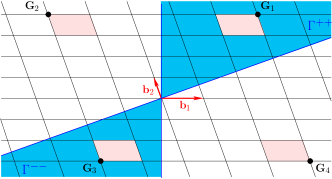
For the multidimensional case we use a similar idea: we bound the value of by its mean over a unit cell for which is the vertex of furthest away from the origin (see Figure 11). A technical difficulty lays in the fact that this is not always uniquely defined and that the ’s do not form a proper tiling. For instance, for the two-dimensional square lattice, we have
with a similar bound for the cubic lattice. For a non-cubic lattice , a partitioning in octants has to be done instead based on the signs of the quantities , in the spirit of what can be seen on Figure 11 for a two-dimensional non-square case.
Unit cells then overlap in the vicinity of the three planes and . A relatively straightforward but tedious bound on these extra overlaps yields the following:
| (9) |
with the unit cell diameter and
with the convention that . Details of this computation will be published in an upcoming paper.
The bound above is numerically observed to be very pessimistic because it uses values of for , which for a rapidly decaying function are much larger than . In order to obtain a better error, we instead apply this bound to the function .
References
- Mo et al. (2013) J.-O. Mo, A. Choudhry, M. Arjomandi, and Y.-H. Lee, J. Wind. Eng. Ind. Aerodyn. 112, 11 (2013).
- Spethmann et al. (2009) P. Spethmann, C. Herstatt, and S. H. Thomke, Int. J. Prod. Dev. 8, 291 (2009).
- Martin and Martin (2004) R. M. Martin and R. M. Martin, Electronic structure: basic theory and practical methods (Cambridge University Press, 2004).
- Snir et al. (2014) M. Snir, R. W. Wisniewski, J. A. Abraham, S. V. Adve, S. Bagchi, P. Balaji, J. Belak, P. Bose, F. Cappello, B. Carlson, et al., Int. J. High Perform. Comput. Appl. 28, 129 (2014).
- Lejaeghere et al. (2014) K. Lejaeghere, V. Van Speybroeck, G. Van Oost, and S. Cottenier, Crit. Rev. Solid State Mater. Sci. 39, 1 (2014).
- Lejaeghere et al. (2016) K. Lejaeghere, G. Bihlmayer, T. Björkman, P. Blaha, S. Blügel, V. Blum, D. Caliste, I. E. Castelli, S. J. Clark, A. Dal Corso, et al., Science 351, aad3000 (2016).
- Cancès et al. (2012) E. Cancès, R. Chakir, and Y. Maday, ESAIM: M2AN 46, 341 (2012).
- Chen et al. (2013) H. Chen, X. Gong, L. He, Z. Yang, and A. Zhou, Adv. Comput. Math. 38, 225 (2013).
- Chen and Schneider (2015a) H. Chen and R. Schneider, ESAIM: M2AN 49, 755 (2015a).
- Chen and Schneider (2015b) H. Chen and R. Schneider, Comm. Comput. Phys. 18, 125 (2015b).
- Kaye et al. (2015) J. Kaye, L. Lin, and C. Yang, Comm. Math. Sci. 13, 1741 (2015).
- Cancès et al. (2016) E. Cancès, G. Dusson, Y. Maday, B. Stamm, and M. Vohralík, J. Comput. Phys. 307, 446 (2016).
- Cancès et al. (ressa) E. Cancès, G. Dusson, Y. Maday, B. Stamm, and M. Vohralik, Math. Comput. (in pressa).
- Cancès et al. (ressb) E. Cancès, V. Ehrlacher, D. Gontier, A. Levitt, and D. Lombardi, Numer. Math. (in pressb).
- Chupin et al. (2020) M. Chupin, M.-S. Dupuy, G. Legendre, and E. Séré, arXiv:2002.12850 (2020), 2002.12850 [math.NA] .
- Dai et al. (2017) X. Dai, Z. Liu, L. Zhang, and A. Zhou, SIAM J. Sci. Comput. 39, A2702 (2017).
- Rohwedder and Schneider (2011) T. Rohwedder and R. Schneider, J Math Chem 49, 1889 (2011).
- Zhao et al. (2015) Z. Zhao, Z. Bai, and X. Jin, SIAM J. Matrix Anal. Appl. 36, 752 (2015).
- Cohen and Bergstresser (1966) M. L. Cohen and T. K. Bergstresser, Phys. Rev. 141, 789 (1966).
- Goedecker et al. (1996) S. Goedecker, M. Teter, and J. Hutter, Phys. Rev. B 54, 1703 (1996).
- Hartwigsen et al. (1998) C. Hartwigsen, S. Goedecker, and J. Hutter, Phys. Rev. B 58, 3641 (1998).
- Rohwedder and Schneider (2013) T. Rohwedder and R. Schneider, ESAIM: Math. Model. and Num. Anal. 47, 1553 (2013).
- Blöchl (1994) P. Blöchl, Phys. Rev. B 50, 17953 (1994).
- Saad (2011) Y. Saad, Numerical Methods for Large Eigenvalue Problems: Revised Edition, Classics in Applied Mathematics (Society for Industrial and Applied Mathematics, 2011).
- Kresse and Furthmüller (1996) G. Kresse and J. Furthmüller, Phys. Rev. B 54, 11169 (1996).
- (26) M. F. Herbst and A. Levitt, “Density-functional toolkit,” Accessed on 08 April 2020.
- Bezanson et al. (2017) J. Bezanson, A. Edelman, S. Karpinski, and V. Shah, SIAM Rev. 59, 65 (2017).
- (28) M. F. Herbst, A. Levitt, and E. Cancès, “Implementation of a posteriori error estimates for non-self-consistent Kohn-Sham equations,” Accessed on 14 April 2020.
- Goerisch and He (1990) F. Goerisch and Z. Q. He, in Computer arithmetic and self-validating numerical methods (Basel, 1989), Notes Rep. Math. Sci. Engrg., Vol. 7 (Academic Press, Boston, MA, 1990) pp. 137–153.
- Babuška and Osborn (1991) I. Babuška and J. Osborn, in Handbook of numerical analysis, Vol. II, Handb. Numer. Anal., II (North-Holland, Amsterdam, 1991) pp. 641–787.
- Heuveline and Rannacher (2001) V. Heuveline and R. Rannacher, Adv. Comput. Math. 15, 107 (2001).
- Mehrmann and Miedlar (2011) V. Mehrmann and A. Miedlar, Numer. Linear Algebra Appl. 18, 387 (2011).
- Kuznetsov and Repin (2013) Y. A. Kuznetsov and S. I. Repin, J. Numer. Math. 21, 135 (2013).
- Bank et al. (2013) R. E. Bank, L. Grubišić, and J. S. Ovall, Appl. Numer. Math. 66, 1 (2013).
- Carstensen and Gedicke (2014) C. Carstensen and J. Gedicke, Math. Comp. 83, 2605 (2014).
- Liu (2015) X. Liu, Appl. Math. Comput. 267, 341 (2015).
- Cancès et al. (2018) E. Cancès, G. Dusson, Y. Maday, B. Stamm, and M. Vohralík, Numer. Math. 140, 1033 (2018).
- Gallistl (2014) D. Gallistl, Comput. Methods Appl. Math. 14 (2014).
- Gallistl (2015) D. Gallistl, Numer. Math. 130, 467 (2015).
- Dai et al. (2015) X. Dai, L. He, and A. Zhou, IMA J. Numer. Anal. 35, 1934 (2015).
- Bonito and Demlow (2016) A. Bonito and A. Demlow, SIAM J. Numer. Anal. 54, 2379 (2016).
- Boffi et al. (2017) D. Boffi, D. Gallistl, F. Gardini, and L. Gastaldi, Math. Comp. 86, 2213 (2017).
- Haynsworth (1968) E. V. Haynsworth, Linear Algebra Appl. 1, 73 (1968).
- IEE (2018) IEEE Std 1788.1-2017 , 1 (2018).
- Sanders et al. (2020) D. P. Sanders, L. Benet, E. Gupta, B. Richard, et al., “JuliaIntervals/IntervalArithmetic.jl: v0.17.0,” (2020).
- (46) A. Noack et al., “Generic numerical linear algebra in Julia,” Accessed on 08 April 2020.
- (47) S. G. Johnson, A. Noack, Y. Ma, et al., “Fourier transforms written in Julia,” Accessed on 08 April 2020.
- (48) J. Sarnoff et al., “DoubleFloats.jl: math with more good bits,” Accessed on 14 April 2020.
- Dusson and Maday (2017) G. Dusson and Y. Maday, IMA Journal of Numerical Analysis 37, 94 (2017).